




No CrossRef data available.
OPTIMIZATION AND OPTIMALITY OF (s,S) STOCHASTIC INVENTORY SYSTEMS WITH NON-QUASICONVEX COSTS
Published online by Cambridge University Press: 06 March 2006
Abstract
This article considers the optimization and optimality of single-item/location, infinite-horizon, (s,S) inventory models. Departing from the conventional approach, we do not assume the loss function describing holding and shortage costs per period to be quasiconvex. As the existing optimization algorithms have been established on the condition of quasiconvexity, our goal in this article is to develop a computational procedure for obtaining optimal (s,S) policies for models with general loss functions. Our algorithm is based on the parametric method commonly used in fractional programming and is intuitive, exact, and efficient. Moreover, this method allows us to extend the optimality of (s,S) policies to a broader class of loss functions that can be non-quasiconvex.
Information
- Type
- Research Article
- Information
- Probability in the Engineering and Informational Sciences , Volume 20 , Issue 2 , April 2006 , pp. 287 - 306
- Copyright
- © 2006 Cambridge University Press
1. INTRODUCTION
The (s,S) type of replenishment policy, also known as the Min-Max control rule, is widely implemented in single-item/location inventory systems. An (s,S) policy instructs that whenever the inventory position (on-hand stock plus outstanding orders minus any backorders, at review) drops to s, which is the reorder level, or below, an order is placed to raise it back up to S, which is the order-up-to level.
In the evaluation of any inventory models, including (s,S) systems, generally two cost components are considered: the ordering cost and the holding-shortage cost, where the second component is often referred to as the loss function. The optimization of an (s,S) system means finding a pair of s and S parameters to minimize the long-run average cost (per period) or discounted total cost. An assumption that is commonly made about (s,S) inventory models is that the expected loss function is convex or quasiconvex in the inventory position. (Quasiconvexity means the existence of an inventory position above which the function is nondecreasing and below which it is nonincreasing.) Most of the research that has been conducted on optimization is grounded on such a condition.
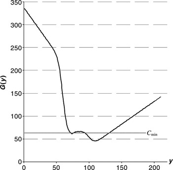
However, this condition is unwarranted in general, and when it is violated, the existing approaches are inoperative. Violation likely occurs when the shortage cost is nonlinear in the inventory positions; for example, when each unit that is backordered incurs a fixed cost, regardless of how long the unit remains in a backlog, or when a fixed cost is incurred whenever there is any backlog on the books in the period, regardless of the volume of the backlog that accumulates. These two types of cost have long been recognized as the shadow costs of fill-rate and ready-rate service constraint, respectively. The fill rate is defined as the fraction of demand that is fulfilled on time, and the ready rate measures the portion of periods during which no shortage occurs. In Section 2.3 we provide an example in which the loss function is non-quasiconvex (see Fig. 1).

Non-quasiconvexity and random lead time.
This article aims to address models with a non-quasiconvex loss function. We have two objectives: first, to identify the conditions under which the (s,S) policy remains globally optimal even in a model with a non-quasiconvex loss function, and, second, to develop a computational procedure for optimizing (s,S) policies in such a generalized model. To fulfill the first objective, we extend the optimality result for the (s,S) policy by identifying a class of non-quasiconvex loss functions that can retain the optimality of (s,S) policies among all policies. Even though the (s,S)-type policy might be suboptimal for models with general loss functions, it is practically adequate because of its simplicity (see Zipkin [21] and Ballou [1]). Therefore, the optimization algorithm alone is of significance. To fulfill the second objective, we propose a descent-search algorithm based on the fractional programming approach that transforms the original model into a parametric problem through an auxiliary function. Emulating a cutting method, the algorithm based on the fractional programming approach is intuitive and easy to initialize and finds the optimal solution efficiently.
The auxiliary function measures the difference between the cost from an (s,S) policy and an artificial, or dummy, cost. The algorithm carries out a search in a three-dimensional space (γ,s,S), where γ denotes the dummy cost. It commences with an easily obtainable value of γ, which is also an upper bound of the optimal long-run average cost Cmin. At each dummy cost level γ, the auxiliary function is evaluated at a few reorder points and various order-up-to levels. When the sign of the auxiliary function becomes negative, the dummy cost is updated. As the dummy cost is lowered to Cmin, both s and S reach their optimal values, and the search ends.
There is a rich body of literature on single-item (s,S) inventory control systems. A significant result from inventory theory is the optimality of (s,S) policies in various models. Using the concept of K-convexity, Scarf [13] provided the first optimality result in a finite horizon setting with setup costs. Iglehart [9] extended this result to an infinite horizon setting. These two seminal articles assumed that the loss function is convex in inventory positions. Veinott [17] adopted a different approach and obtained the optimality result for both finite and infinite horizon problems under a different set of assumptions: The loss function is quasiconvex, but demand over time is stochastically nondecreasing. This article thus generalizes the optimality results that are established by Iglehart [9] and Veinott [17] for the infinite horizon setting. Many authors have extended the previous results to different problem settings (e.g., Song and Zipkin [16] and Sethi and Cheng [14] in a Markovian demand environment, and Li, Xu, and Hayya [10] in a random supply context). Since the study of Veinott and Wagner [18], the optimization of infinite horizon, stationary (s,S) models has aroused much interest in the literature. Zheng and Federgruen [20] (ZF hereafter) have developed the best solution procedure so far for cases with quasiconvex loss functions. More recently, Feng and Xiao [7] (FX hereafter) proposed an alternative to ZF's. The method in the present article represents a further generalization of these two algorithms.
The rest of the article is organized as follows. Section 2 specifies the inventory model and shows an example in which a loss function is non-quasiconvex. Section 3 explores the properties of the method and proposes the algorithm. We address the optimality of (s,S) policies with non-quasiconvex loss functions in Section 4. Section 5 reports numerical examples, and Section 6 summarizes the article. A list of symbols is included in Section 2 for ease of reading.
2. THE INVENTORY MODEL AND LOSS FUNCTIONS
2.1. Notation
Symbols that are used throughout the sections are summarized here, whereas those that are used briefly will be defined locally.

2.2. A Periodic Review Inventory System
We consider an infinite horizon, periodic-review inventory system that faces discrete-valued independent and identically distributed (i.i.d.) demands. Demand that is not met immediately is fully backlogged and will be fulfilled on a first-come–first-served basis. The system replenishes inventory according to an (s,S) policy with a constant lead time of L periods. (The random lead time will be introduced after the basic model has been formulated.) The sequence of events in each period is as follows: The inventory is reviewed, an order that was placed L periods ago is received, an ordering decision is made, and the demand in the period is then subtracted out of the inventory. These events are supposed to happen at the beginning of each period.
It is well known (e.g., Veinott and Wagner [18], and ZF [20]) that

For ease of analysis, we impose a minor condition on G(y), which is also assumed in most of the previous work:
Assumption 1: limy→±∞ G(y) > K + G(y0).
It should be noted that when L is a random variable, G(y) should be understood as the expected loss function over demand and the lead time

Under the conditions that are explicated by Zipkin [21], the distribution of demand over the deterministic lead time L is just replaced by the distribution of total demand over the stochastic lead time. The conditions are met when the system faces an exogenous, sequential supply source in which the lead times are i.i.d. over time and no order-crossing occurs.
We also assume that demand takes a discrete value, but that continuous distributions can be discretized with an arbitrary precision.
2.3. An Example of Non-quasiconvex Loss Function
In a recent article, Rosling [11] considered loss functions with nonlinear shortage costs. His basic model is a periodic-review model that is almost identical to ours; in his model, two nonlinear shortage (or backorder) costs are added to the traditional linear shortage cost. Here, we only give their mathematical expressions and refer the reader to Rosling [11] for a further explanation.
Suppose that the inventory position after possible ordering is y; then

where

, which is the shortage cost that accumulates at a constant rate proportional to the number of backorders on the books;

, which is the cost that occurs only for the incremental backorders that arise in a period (Hadley and Whitin [8], Chen and Zheng [3], and Bashyam and Fu [2]); Bb(y) = 1 − ΦL+1(ξ), which is the cost that is incurred whenever there are any backorders in a period (Silver, Pyke, and Peterson [15]); and H(y) is the expected holding cost (per period). (For brevity, we simply denote G(y|L) by G(y).) Setting π = b = 0, we have a loss function with a traditional linear backorder cost. Generally, b and π are viewed as Lagrangian multipliers, or shadow costs, of the ready and fill rates, respectively.
Assuming that the holding cost incurs at a constant rate and that the lead time for replenishment orders is constant, Rosling [11] showed that when p,π,b ≥ 0, G(y) is quasiconvex if Φ(ξ) is log-concave. This condition is met by many demand distributions, including the Normal, Poisson, Negative Binomial, gamma family, Weibull, and beta with parameters (r,q) such that both r and q ≥ 1. However, there are significant exceptions. Take an example that is given in Eppen and Martin [5]: The demand of each time period is normally distributed with mean 20 units and variance 10 (units)2. The lead time (in periods) can take on the values 2 and 4 with probabilities of 0.8 and 0.2, respectively. In such a case, the (expected) loss function fails to be quasiconvex when the backlogging cost is nonlinear. Figure 1 illustrates a case in which p = $2/unit/period, π = 0, b = $200/period, and the holding cost rate is $1/unit/period. (The line that is associated with Cmin will be explained later.)
Although the loss function can be non-quasiconvex in the inventory position, G(y) generally increases monotonically after y becomes sufficiently large, and it is nonincreasing when y < 0. For example, a test can be carried to see whether G(y) will become monotonic. Suppose that H(y) is convex. If H(y1 + 1) − H(y1) ≥ pBp(y1) + πBπ(y1) + bBb(y1) (see (1)), then G(y) is increasing for all y > y1.
3. FINDING AN OPTIMAL (s,S) POLICY
When the loss function G(y) is quasiconvex, one can apply the algorithm developed by ZF [20] or by FX [7] to search for an optimal (s,S) policy. These algorithms are exact and efficient. Here, our focus is on a model with a non-quasiconvex loss function, and we will discuss whether it is possible to extend ZF's algorithm to the current setting later.
We will first reveal the properties of an optimal (s,S) policy and then derive an algorithm for its computation.
3.1. Auxiliary Function Method and Preliminary Results
To elaborate our computational procedure, we introduce a dummy cost γ, which is assumed to be in the range γ ∈ A = {γ : G(y0) ≤ γ ≤ K + G(y0)}. As will be shown, the assumption about γ can be trivially met (see Section 3.4). We then define an auxiliary function that relates to this γ as follows:

In fractional programming, the problem of minimizing lγ(s,S) over s < S is called a parametric problem. The use of such an approach in inventory theory was first proposed by Feng and Sun [6].
One might think of the dummy cost γ as a budget level per period. Because

is the expected total cost per ordering cycle, the difference

gives the cumulative deficit in operating the system per renewal cycle; that is, if the budgeted cost exceeds the expected operating cost, then there will be a surplus, and if the expected operating cost exceeds the budgeted cost, then there will be a fiscal shortfall. The objective is therefore converted to one that minimizes lγ(s,S).
Our interest in the auxiliary function is due to the fundamental properties of fractional programming regarding the value γ* and the function wγ, which are defined respectively as γ* = {γ ∈ A : mins≤S lγ(s,S) = 0} and wγ = mins<S lγ(s,S). In what follows, we denote by sγ and Sγ the pair that minimize lγ(s,S) under a given γ. We also term (sγ,Sγ) optimal with respect to the auxiliary function; that is,

Lemma 1:
(a) The minimum achievable cost Cmin = γ*, and the function w(γ) is strictly decreasing in γ.
(b) For a given γ ≥ G(y0), if a pair of s and S exists such that lγ(s,S) < 0, then γ is an upper bound of Cmin.
(c) Defining

Cmin ≤ γ1 < γ, γ1 = C(s,S), and lγ1(s,S) = 0. In particular, Cmin = γ* = C(sγ*,Sγ*).
In view of Lemma 1, the minimization of C(s,S) is equivalent to finding a γ ≥ G(y0), such that mins<S lγ(s,S) = 0. Specifically, we begin with an initial dummy cost γ0 ≥ Cmin and then iteratively lower it until the condition mins<S lγ(s,S) = 0 is satisfied.
For later use, we rearrange the auxiliary function

As y0 is a global minimizer of G(y) given a γ ≥ G(y0), it follows that

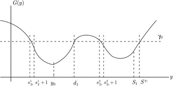
Let P(γ) = {y : G(y + 1) ≤ γ < G(y)}. In Figure 2 (where the curve is smoothed and γ = γ0), there are two elements in P(γ0): sγ01 and sγ02. Lemma 2 shows that P(γ) is the set that contains all potential candidates for sγ. If we denote these candidates as sγ1,sγ2,…, in ascending order of value, then P(γ) = {sγ1,sγ2,…}.

An illustration of candidates for sγ0 and ranges for Sγ0.
Lemma 2:
(a) For any given S such that G(S) < γ, the optimal reorder level sγ satisfies

(b) For a given γ and sγ ∈ P(γ), the optimal order-up-to level Sγ ≤ Sγ, where Sγ = max{y : G(y) ≤ γ}.
Proof: Part (a) follows from the fact that

For part (b), we assume to the contrary that G(Sγ) > γ. Then, following (3),

which implies that

If

, then we have 0 > 0, which is an impossible event. Thus,

, leading to

which is a contradiction of (4). Thus, the lemma follows. █
Lemma 2 implies that sγ ∈ P(γ). Because of Assumption 1 and the assumption that G(y0) ≤ γ ≤ K + G(y0), the set P(γ) is clearly nonempty and finite. It can easily be seen that the lower bound of s* is sγ01. Furthermore, not every value of y ≤ Sγ can be an effective order-up-to level. For example, in Figure 2, it can be seen that for an (sγi,S) to be optimal, y0 ≤ S ≤ d1 or S > sγ2, where d1 = min{y > sγ1 : G(y) ≤ γ} and i = 1 or 2. There are more unattractive candidates for Sγ that can be eliminated. However, for notational simplicity, we will compromise some efficiency by ignoring these properties in the sequel algorithm design.
Lemma 2 represents the major extension of the work of FX. In the rest of the section, we discuss a method for the upgrading of order-up-to levels and when to end the search. Interestingly, the properties that are revealed in these discussions are direct extensions of those of FX and in fact these discussions do not engage the loss function.
We close this subsection with a brief comparison of the average-cost approach of ZF and our auxiliary-function approach. By Eq. (6) in ZF and by the proof of Lemma 1 in Zheng [19], one can derive a lower bound for s* and an upper bound for S*, respectively. If their algorithm starts with an initial policy that gives γ0 and ends with the lowest average cost Cmin being identified, then these two bounds coincide with our sγ01 and SCmin. However, a full enumeration within these bounds is required in their approach, whereas our approach allows a more efficient search. The difference arises from the fact that they directly use the cost function C(s,S) to design their algorithm, whereas we use the auxiliary function lγ(s,S). Although both functions vary with the policy (s,S), lγ(s,S) has a simpler form.
3.2. Updating Order-up-to Levels
In this subsection, we discuss a method for updating the optimal order-up-to level in conjunction with the upgrading of the dummy cost. We use Figure 2 to demonstrate how the dummy cost will be upgraded in our algorithm. Under γ = γ0, suppose that for all S < S1, lγ(sγi,S) ≥ 0, i = 1 or 2, but lγ(sγ1,S1) < 0 (or lγ(sγ2,S1) < 0). We then immediately upgrade the dummy cost from γ to γ1 = C(sγ1,S1) (or C(sγ2,S1)). In the sequel, when we say that the algorithm updates the dummy cost γ at pair (s1,S1), we mean that under γ, for all the potential (s,S) policies with s < S < S1, lγ(s,S) ≥ 0, but by raising S to S1, a pair (s1,S1) emerges such that lγ(s1,S1) < 0, where s1 < S1,s1 ∈ P(γ) and S1 ≤ Sγ. This is how and when the dummy cost γ is upgraded in the proposed algorithm: As soon as lγ(s,S) turns negative, the dummy cost is lowered from γ to γ1. The following discussion is based on such an upgrading scheme.
Now suppose that the dummy cost γ is upgraded to γ1 by a given policy (s1,S1), where s1 ∈ P(γ), and a new set P(γ1) is formed as sγ11 < sγ12 < ···. Do we need to evaluate all (sγ1i,S1 − j) policies, where j = 1,2,…? The answer is no, which is deduced from the following lemma.
Lemma 3: Suppose that γ is upgraded to γ1 < γ by a policy (s1,S1), where s1 ∈ P(γ), S1 < Sγ, and

Then for any sγ1i ∈ P(γ1) and y < S1, we have

Proof: Apparently, given s1 < S1, lγ(s1,S1), as a function of γ > 0, strictly decreases in γ. As a result, for sγ1i ∈ P(γ1) and y < S1,

The last inequality results from the updating scheme of the dummy cost that was described earlier. █
3.3. Identifying Cmin and an Optimal (s,S) Policy
Once γ is upgraded to γ* = Cmin, the algorithm needs to be terminated and an optimal (s,S) policy identified. This subsection discusses when the algorithm should terminate.
Lemma 4: Suppose that the algorithm upgrades the dummy cost γ at (s1,S1) to γ1 = C(s1,S1) where s1 ∈ P(γ). In addition, suppose that for all s ∈ P(γ1) and S1 ≤ y ≤ Sγ1,

Then, γ* = Cmin = γ1, s* = sγ* = s1, and S* = Sγ* = S1.
Proof: In view of Lemma 3, for a case in which s ∈ P(γ1) and y < S1, lγ1(s,y) ≥ 0. With these assumptions, we have

and, thus, γ1 ≤ Cmin. However, as γ1 = C(s1,S1) ≥ Cmin = γ*, we have γ1 = γ*. Furthermore, as lγ*(s1,S1) = 0, we can conclude that s* = sγ* = s1 and S* = Sγ* = S1. █
This lemma indicates that in the final γ upgrading attempt, the search will continue until Sγ*, which is the largest order-up-to level to be evaluated, is reached.
3.4. The Algorithm
We now present the descent-search algorithm, which starts with an initial dummy cost γ0 = C(s,S) ≤ K + G(y0). This kind of dummy cost can be easily obtained. For instance, when s = y0 − 1 and S = y0,

can be selected as γ0. It is generally easy to locate sγ01; for example, we can start with y = 0. If G(0) > γ0, then sγ01 ≥ 0, and if G(0) ≤ γ0, then sγ01 < 0. This is because G(y) is decreasing when y < 0. We assume that a number y is also available so that for y ≥ y (see the remark at the end of Section 2.3), G(y) is increasing. In finding y, a global minimizer of G(y), y0, also becomes known. In the algorithm, we do not describe how Sγ is computed, because such a procedure is straightforward. The algorithm will be called the descent-search algorithm, because the dummy cost is lowered after each iteration.
Descent-search algorithm
[bull ] Step 0 (Initialization)
Let γ1 = γ0,γ* = γ1,I = Ø, and Cmin = γ1. Compute sγ11 and add sγ11 into set I. Let s = sγ11, and S = s + 1. s* = s, and S* = S. Go to Step 1.1.
[bull ] Step 1
1.1. For all s ∈ I, compute lγ1(s,S) and mins∈I lγ1(s,S). If mins∈I lγ1(s,S) < 0 for s = s′ ∈ I, then go to Step 2.1. Otherwise (i.e., mins∈I lγ1(s,S) ≥ 0), go to Step 1.2.
1.2. Let S := S + 1. If S > Sγ1, then go to Step 3. If G(S − 1) > γ1 ≥ G(S), then add S − 1 into I. Go to Step 1.1.
[bull ] Step 2 (Updating the dummy cost)
2.1. Update γ1 by computing

let s* = s and S* = S. Go to Step 2.2.
2.2. Let S := S* and compute sγ11. Set I = Ø and add sγ11 into I. Go to Step 1.1.
[bull ] Step 3 (Termination)
Stop with Cmin = γ* and the optimizing policy (s*,S*).
The algorithm works as follows. It starts with γ0. The set of potential reorder levels associated with the dummy cost γ0 consists of sγ0i, i = 1,2,…,τ. The set I contains the levels in P(γ0) that are currently used for evaluation. At the very beginning, the set I contains just one reorder level s = sγ01, and the algorithm begins with the computation of lγ0(sγ01,sγ01 + 1).
Step 1.1 evaluates all lγ1(s,S), with S being fixed but s being taken from I. The minimum of lγ1(s,S) and lγ1(s′,S) is then obtained. Once this minimum becomes negative, the algorithm immediately upgrades γ1 in Step 2 by the (s′,S) policy.
If the minimum of lγ1() is nonnegative, then the algorithm proceeds to Step 1.2. The current order-up-to level S is replaced by S + 1; meanwhile, a test is carried out to see whether S > Sγ. If this is the case, then the algorithm jumps to Step 3 in terms of Lemma 2b. Otherwise, another test is undertaken to see whether G(S − 1) > γ ≥ G(S) and S − 1 can be added to I (by Lemma 2a). Afterward, the algorithm goes back to Step 1.1.
In Step 2.1, the dummy cost γ1 is upgraded to a “new” γ1 by (s′,S) according to Lemma 1b. The “default” optimal policy (s*,S*) and dummy cost γ* are also updated at this step. In view of Lemma 3, the search for a “new” order-up-to level begins with S* in Step 2.2. With the new dummy cost, the algorithm regenerates the first candidate for the optimal reorder level and adds it into set I.
Finally, the computation comes to an end in Step 3, in which the optimal (s,S) policy and Cmin are identified. The reason why it is possible to have Cmin in Step 3 is given by Lemma 4.
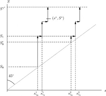
We use Figures 2 and 3 to illustrate how the algorithm is executed. At γ0, the algorithm first searches for the smallest candidate for sγ0 (i.e., sγ01). It then sets S0 = sγ01 + 1 to start the process that will upgrade γ0. As S0 is increased to S0′, sγ02(= S0′ − 1) is encountered, and both (sγ01,S0′) and (sγ02,S0′) are evaluated. As S is further increased to S1, lγ0(sγ0i,S1) turns to a negative value (i = 1 or 2) and γ0 is lowered to γ1. Under γ1, two candidates of sγ1 are identified: sγ11 and sγ12. The next around of dummy-cost upgrading then begins with the evaluation of both (sγ1i,S1), i = 1 and 2. (For the reason for skipping the order-up-to level below S1, refer to the beginning of Section 3.2.) This process continues until γ1 is upgraded, and eventually the optimal policy (s*,S*) is confirmed after Sγ* has been reached.

A typical execution of the algorithm.
It is well recognized that an evaluation of C(sγ11,S), and hence lγ1(sγ11,S), is a major operation. We thus call each computation of lγ1(sγ11,S) a critical evaluation. Each time S advances by a unit, lγ1(sγ11,S) has to be “completely” recalculated, with virtually nothing from the previous evaluation of lγ1(sγ11,S − j), j ≥ 1, being usable. Therefore, the complexity of the algorithm is mainly determined by the number of critical evaluations (NCE) of lγ1(sγ11,S) pertaining to different S. Because the NCE is determined by the cost structure and initial dummy cost γ0, the complexity of the algorithm is dependent on the holding-shortage cost and the initial dummy cost. Given an initial dummy cost of γ0, the NCE can be greater than (Sγ* − sγ01), because if the dummy cost is upgraded at (s′,S) from γ to γ1, then S will probably be evaluated twice. Nevertheless, the NCE is bounded by 2(Sγ* − sγ01).
Although the main computational effort relates to the NCE, after each updating of γ, a set of new candidates for the optimal reorder level must be relocated. For this reason, we introduce another criterion: the number of dummy profit cost upgrades (NDC), which measures the number of times that γ is upgraded. Both the NCE and NDC will be obtained later in numerical examples.
We conclude this section with a brief discussion of the complexity of the algorithm. Note that the algorithm ends in a finite number of iterations, because each γ upgrading will push s and/or S forward by at least one. Also note that when the loss function is quasiconvex, the algorithm essentially collapses to that proposed by FX. Note that FX's algorithm has the same complexity as ZF's—about twice the effort that is required to evaluate a specific (s,S) policy. When the loss function is non-quasiconvex, additional effort is required to evaluate perhaps several (sγi,S) policies simultaneously for each S. However, according to ZF, in calculating C(sγ1,S), the C(sγi,S) are readily available, where i = 2,… and sγi > sγ1. Thus, our algorithm has roughly the same complexity as the two other algorithms (see Chen and Feng [4] for more details).
4. OPTIMALITY OF (s,S) POLICIES: AN EXTENSION
This section extends the optimality analysis of (s,S) policies to a larger class of loss functions, taking a quasiconvex loss function as a special case.
Suppose that we have applied our algorithm to the loss function G(y) and obtained the long-run average cost, Cmin, of the optimal (s,S) policy (i.e., γ* = Cmin). Without causing any confusion and for notational convenience, we drop * from γ* in the rest of this section. We denote by (s*,S*) the optimal (s,S) policy, as in the previous sections. The (s,S) optimization analysis confines the optimal parameters (s*,S*) between sγ1, the smallest or the first candidate for the optimal reorder level, and an upper bound, Sγ, of S*, which is defined by G(Sγ) ≤ γ < G(y) for all y > Sγ.
The class of loss functions that we are interested in is defined as follows.
Definition 1. A loss function G(y) is called first reorder-point optimal if, under γ, the optimal (s*,S*) policy is such that s* = sγ1 < S*, and for s* < x ≤ Sγ,

In words, a first reorder-point optimal loss function requires that lγ(sγ1,S*) = 0 and lγ(s,S) ≥ 0 for all s < S. Note that the right-hand side of (5) is a weighted average of G(s* + 1),G(s* + 2),…,G(x), where Sγ ≥ x > s* = sγ1. This weighted average can be interpreted as the long-run average cost of the policy (s*,x) as if there were no setup cost. Take Figure 2 as an illustration. Suppose that γ = γ0 in the figure. If G(y) is first reorder-point optimal, then it must follow that s* = sγ01, and the right-hand side of (5) is bounded by γ0 for all x = sγ01 + 1,…,Sγ0.
It is obvious that a quasiconvex loss function is first reorder-point optimal. Another type of loss function that is first reorder-point optimal might be referred to as a γ-uniformly-bounded loss function.
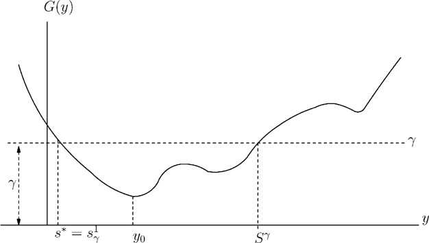
Definition 2: A loss function G(y) is called γ-uniformly-bounded if for any pair of integers a < b, max{G(a),G(b)} ≤ γ implies G(y) ≤ γ for all a ≤ y ≤ b.
Figure 4 depicts an example of a γ-uniformly-bounded function. If G(y) is found to be γ-uniformly-bounded, then s* = sγ1, and for all x, s* ≤ x ≤ Sγ, γ ≥ G(x). As a result, (5) is met for all x ∈ (s*,Sγ], and the loss function is first reorder-point optimal.

An illustration of a γ-uniformly-bounded function.
To examine whether the loss function, G(y), is first reorder-point optimal, we need to (1) apply our algorithm to obtain the (s*,S*) policy and its cost γ = Cmin, (2) check whether s* = sγ1, and (3) confirm whether (5) holds for every x ∈ (s*,Sγ] should s* = sγ1 be true.
First reorder-point optimal loss functions lead to the global optimality of the (s*,S*) policy, as is claimed by the ensuing theorem.
Theorem 5: Suppose that the loss function G(y) is first reorder-point optimal. The (s*,S*) policy is then the optimal policy of all of the admissible ordering policies.
Proof: According to the basic theory of dynamic programming (see [12, Chap. V, Thm.2.1]), the average cost γ = Cmin is the minimum average that can be attained by any admissible policy if a bounded function h(y) exists such that the following optimality equation holds:

where a stationary policy that chooses actions to minimize the right-hand side of (6) is admissible, and δ{·} is an indicator function of the event described by {·}: if the argument is true (i.e., y > x), then δ = 1; otherwise, y = 0. This set of conditions is often called an optimality criterion. From Ross [12], if (6) holds, then the implied policy that minimizes the right-hand side of (6) is optimal among all admissible policies and γ is its long-run average cost. Consequently, the (s*,S*) policy is also optimal, because it also achieves γ. It should be noted that the implied policy and the (s*,S*) policy need not be the same.
It seems impossible to construct a bounded function h(x) such that the optimal equation (6) holds with γ. For this reason, we adopt the following argument that was proposed by Zheng [19], who provided a simple proof for the optimality of (s,S) policies in models with quasiconvex loss functions. Suppose that inventory can be returned to the supplying source; that is, the firm can place orders of negative quantities. Returning of any quantity incurs the same setup cost as placing an order for a positive quantity, but there is no variable cost. Allowing the firm to reduce excess inventory might lower the long-run average cost. A model with such an additional option will be called a relaxed model. If we can verify that the minimum cost that the relaxed model can achieve is still γ, then the (s*,S*) policy is globally optimal in the original model.
With a return option, the optimality equation (6) has to be modified for the relaxed model:

To ensure (7), we construct a function h(x) as follows:

where lγ() is as previously defined.
First, we show that such a function h(x) is bounded; in particular,

for all integers x. This is true by the definition of h(x) when x ≤ s*. For x ∈ (s*,Sγ], as it has already been shown in Section 4 that lγ(s*,x) ≥ lγ(s*,S*) = 0, h(x) = lγ(s*,x) ≥ 0. To confirm that h(x) ≤ K, note that for every x ∈ (s*,Sγ],

By (2), we thus have

for s* < x ≤ Sγ.
When x > Sγ, because h(x) ≤ K by construction, we only need to confirm that h(x) ≥ 0. Applying induction, we begin with x = Sγ + 1. Note that either

because G(Sγ + 1) > γ, or h(Sγ + 1) = K. In either case, h(Sγ + 1) > 0, which suffices for the induction. Thus, K ≥ h(x) > 0 for x > Sγ.
We now verify the optimality equation (7). By defining a new function as

the optimality equation (7) can be rewritten as

Note that for s* < x ≤ Sγ, V(x) = lγ(s*,x). Because G(x) > γ when x ≤ s* and x > Sγ, it is implied by the nonnegativity of h(x) that H(x) > 0 for those x. When s* < x ≤ Sγ, V(x) = h(x) = lγ(s*,x) ≥ 0 and the minimum of V(x) is achieved at x = S*, where V(S*) = h(S*) = 0. Therefore, the criterion (7) is equivalent to

An optimal action that minimizes the right-hand side of (9) is to decide between staying at the current inventory position x or adjusting x to S*, depending on which yields a smaller value.
To show criterion (9), the following three ranges are considered: (1) x ≤ s*, (2) S* < x ≤ Sγ, and (3) Sγ < x. In range (1), V(x) = G(x) − γ + K > K, which indicates that an optimal policy is to set y = S* ≥ x (i.e., to place an order of (S* − x) units). In range (3), h(x) = min(K,V(x)) by definition, implying an optimal policy of either returning some inventories to lower x to S* or doing nothing. Finally, in range (2), h(x) = V(x) ≤ K, suggesting not to do anything. Hence, the optimality equation is met for all x, and the optimal policy at each x is admissible. This concludes that the minimum average cost is γ in the relaxed model and, consequently, that the (s*,S*) policy is also optimal in the relaxed and original models. █
This argument is intuitive. Note that the optimal policy minimizing the right-hand side of (7) differs from the (s*,S*) policy only in a finite number of initial periods. This is because when the initial inventory position is above Sγ, the former policy might issue an order for a negative quantity, whereas the latter policy does nothing. In either case, the inventory position will fall to Sγ or below in a finite number of periods, after which the two policies work identically. In terms of long-run average cost, both policies obtain γ, because the cost difference in a finite number of initial periods does not affect the performance in the long run.
Theorem 5 broadens the optimality of the (s,S) ordering policies in the sense that the quasiconvex loss functions become just a subclass of the first reorder-point functions. We have thus extended the optimality result of Iglehart [9] and Veinott [17].
5. NUMERICAL EXAMPLES
The descent algorithm was used to solve several sets of problems to observe its operating characteristics. In the algorithm implementation, a module is included to test whether the first-reorder-point condition is met in each instance.
In all of the examples, the period demand follows the Normal distribution (μ,σ2), and the lead time is either two periods (w.p. 0.8) or four periods (w.p. 0.2). We consider only one nonlinear shortage cost: in Eq. (1), p > 0 and b > 0, but π = 0. In addition, we take the linear holding cost with a rate h > 0.
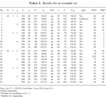
The results for these problems are displayed in Table 1, in which the first block records the cost parameter values; the second block displays three bounds: s0 and Su, which represent the first candidate of reorder point that is associated with C0 (the initial dummy cost), and the upper bound of S* associated with Cmin; and the quasiconvexity of the loss function is tested and indicated under “CoV,” where nq stands for non-quasiconvex and qu stands for quasiconvex. The third block reports the optimal solution: the optimal policy (s*,S*) and the minimum cost Cmin. The column under “Opt” indicates whether the (s*,S*) policy is globally optimal. If the first-reorder-point condition is satisfied, then the answer is “Yes”; otherwise, the optimality is unknown. The column NCE reports the number of times that the auxiliary function is evaluated, and the NDC displays the number of dummy cost upgrades. As explained earlier, these two numbers measure the computational effort that is expended in obtaining the optimal policy parameters. The global minimizer of G(y) is not reported, although in all examples, C0 = C(y0 − 1,y0).
Results for an example set

In all instances except one, the (s*,S*) policy is tested to be globally optimal. In the only exception, example 2, the test is inconclusive, which is shown graphically in Figure 1. As can be seen from Table 1 and Figure 1, the optimal reorder point s* does not take the first candidate for the reorder point. The achieved ready rates that were calculated but not reported here are between 0.64 and 0.97. Several different sets of problem data were also computed, for example, with different demand and lead-time distributions, but the results are similar and are thus not reported here. In general, when the setup cost K or the holding cost h is relatively large, the optimality test of the (s,S) policy is more conclusive, because the average cost is high and, hence, the loss function is γ-uniformly-bounded. Although it is generally true that the smaller the nonlinear shortage cost p or π is, the more likely it is that the first-reorder-point condition is met, there are exceptions. Comparing Example 2 with Example 3 in Table 1, we see that as b decreases, the condition is actually violated.
6. CONCLUDING REMARKS
In this article we develop an intuitive and efficient algorithm for computing an optimal (s,S) policy. Unlike most of the existing methods, this algorithm can handle models with non-quasiconvex loss functions. Based on a parametric problem associated with the original optimization problem, the algorithm was devised using an auxiliary function with a dummy cost. It starts with an easily identifiable dummy cost and then upgrades the dummy cost reiteratively until the optimizing policy is identified. The computational effort is mainly expended on the evaluation of the value of the auxiliary function with each order-up-to level. Because it advances the order-up-to level unidirectionally from left to right, the algorithm is efficient. We also establish conditions under which an (s,S) policy is optimal among all policies in the model with a non-quasiconvex loss function. This result extends the standard model with a quasiconvex loss function and is also readily extendable to other models. However, we refer the reader to Zheng and Federgruen [20] for a detailed discussion of these models.
Acknowledgments
This research was partially supported by Hong Kong RGC/CUHK grant No. 2050310. The authors are grateful to the anonymous referee for constructive comments, which have improved the presentation of the paper. The computational assistance of Mr. Tong Wang is also appreciated.
References
REFERENCES
Ballou, R.H.
(1999).
Business logistics management: Planning, organizing, and controlling
the supply chain,
4th ed.
Upper Saddle River, NJ:
Prentice-Hall.
Bashyam, S. &
Fu, M.C.
(1998).
Optimization of (s,S) inventory systems with
random lead times and a service level constraint.
Management Science
44:
243–256.Google Scholar
Chen, F. &
Zheng, Y.-S.
(1993).
Inventory models with general backorder costs.
European Journal of Operational Research
65:
175–186.Google Scholar
Chen, Y. &
Feng, Y.
(2004).
Optimization and optimality of (s,S) stochastic
inventory systems with non-quasiconvex costs.
Unabridged version,
Department of System Engineering & Engineering Management, The
Chinese University of Hong Kong,
Shatin, Hong Kong, China. Downloadable from www.se.cuhk.edu.hk/yhchen.
Eppen, G.D. &
Martin, R.K.
(1988).
Determining safety stock in the presence of stochastic lead time and
demand.
Management Science
34:
1380–1390.Google Scholar
Feng, Y. &
Sun, J.
(2001).
An algorithm for deriving
(r,R,d,D) inventory replenishment
policy.
Operations Research
49:
1380–1390.Google Scholar
Feng, Y. &
Xiao, B.
(2000).
New algorithms for computing optimal (s,S)
policies in a stochastic single item/location inventory system.
IIE Transactions
32:
1081–1090.Google Scholar
Hadley, G. &
Whitin, T.M.
(1963).
Analysis of inventory systems.
Upper Saddle River, NJ:
Prentice-Hall.
Iglehart, D.
(1963).
Optimality of (s,S) policies in the infinite
horizon dynamic inventory problem.
Management Science
10:
259–267.Google Scholar
Li, Z.,
Xu, S.H., &
Hayya, J.
(2004).
A periodic-review inventory system with supply interruptions.
Probability in the Engineering and Informational Sciences
18:
33–53.Google Scholar
Rosling, K.
(2002).
Applicable cost rate functions for single-item inventory
control.
Operations Research
50:
1007–1017.Google Scholar
Ross, S.
(1983).
Stochastic processes.
New York:
Wiley.
Scarf, H.
(1960).
The optimailtiy of (s,S) policies in the dynamic
inventory problem. In
K. Arrow,
S. Karlin, &
P. Suppes (eds.),
Mathematical methods in the social sciences.
Stanford, CA:
Stanford University Press,
Chap. 22.
Sethi, S. &
Cheng, F.
(1997).
Optimality of (s,S) policies in inventory models
with Markovian demands.
Operations Research
45:
931–939.Google Scholar
Silver, E.A.,
Pyke D., &Peterson,
R.A.
(1998).
Inventory management and production planning and scheduling,
3rd ed.
New York:
Wiley.
Song, J.-S. &
Zipkin, P.
(1993).
Inventory control in a fluctuating demand environment.
Operations Research
41:
351–370.Google Scholar
Veinott, A., Jr.
(1966).
On the optimality of (s,S) inventory policies: New
conditions and a new proof.
SIAM Journal of Applied Mathematics
14:
1067–1083.Google Scholar
Veinott, A., Jr. &
Wagner, H.M.
(1965).
Computing optimal (s,S) inventory policies.
Management Science
11:
690–723.Google Scholar
Zheng, Y.-S.
(1991).
A simple proof for optimality of (s,S) policies in
infinite-horizon inventory systems.
Journal of Applied Probability
28:
802–810.Google Scholar
Zheng, Y.-S. &
Federgruen, A.
(1991).
Finding optimal (s,S) policies is about as simple
as evaluating a single policy.
Operations Research
39:
654–665.Google Scholar
Zipkin, P.
(1999)
Foundations of inventory management.
Singapore:
McGraw-Hill Higher Education, pp.
196–198.
Non-quasiconvexity and random lead time.
An illustration of candidates for sγ0 and ranges for Sγ0.
A typical execution of the algorithm.
An illustration of a γ-uniformly-bounded function.
Results for an example set
 You have
Access
- 3
- Cited by