1 Introduction
Many magnetized astrophysical plasmas – for example, the solar wind and the intracluster medium of galaxy clusters – are turbulent and weakly collisional, with particle mean free paths that are comparable to, or exceed, the scales of plasma motions. Despite this scale hierarchy, it is broadly assumed that such plasmas can be described by single-fluid magnetohydrodynamics (MHD), at least on scales much larger than the plasma’s kinetic microscales (e.g. the ion gyroradius
 $\unicode[STIX]{x1D70C}_{i}$
or skin depth). Indeed, there are certain situations in which this simplification can be justified rigorously (e.g. Kulsrud Reference Kulsrud, Sagdeev and Rosenbluth1983; Schekochihin et al.
Reference Schekochihin, Cowley, Dorland, Hammett, Howes, Quataert and Tatsuno2009). In this work, we show that there exists a significant dynamical effect in weakly collisional plasmas that is not captured by the MHD model. It affects plasmas whose thermal energies are comparable to their magnetic energy,
 $\unicode[STIX]{x1D6FD}\equiv 8\unicode[STIX]{x03C0}p_{0}/B^{2}\gtrsim 1$
(where
 $p_{0}$
is the thermal pressure and
 $B=|\boldsymbol{B}|$
is the magnetic-field strength). This effect, which we call ‘magneto-immutability’, is the tendency of the plasma motions to self-organize so as to resist changes in magnetic-field strength.
Magneto-immutability arises from the dynamical effects of pressure anisotropy,
 $$\begin{eqnarray}\unicode[STIX]{x0394}p\equiv p_{\bot }-p_{\Vert },\end{eqnarray}$$
which is the difference between the thermal pressures perpendicular (
 $\bot$
) and parallel (
 $\Vert$
) to the magnetic field. Pressure anisotropy is generated locally whenever and wherever
 $B$
changes slowly in a plasma with the ion-collision frequency
 $\unicode[STIX]{x1D708}_{c}$
much smaller than the gyrofrequency
 $\unicode[STIX]{x1D6FA}_{i}$
(Chew, Goldberger & Low Reference Chew, Goldberger and Low1956; while the same is true for electrons, ion microphysical parameters are most relevant for the effects studied here). Although pressure anisotropy is well studied in solar-wind plasmas (Kasper, Lazarus & Gary Reference Kasper, Lazarus and Gary2002; Bale et al.
Reference Bale, Kasper, Howes, Quataert, Salem and Sundkvist2009), most authors have focused on microscale kinetic instabilities that are excited if
 $|\unicode[STIX]{x0394}p|$
becomes too large, rather than on the dynamical feedback of
 $\unicode[STIX]{x0394}p$
on the large-scale motions (but see Helander, Strumik & Schekochihin Reference Helander, Strumik and Schekochihin2016; Squire, Quataert & Schekochihin Reference Squire, Quataert and Schekochihin2016; Squire et al.
Reference Squire, Kunz, Quataert and Schekochihin2017a
; Yang et al.
Reference Yang, Matthaeus, Parashar, Haggerty, Roytershteyn, Daughton, Wan, Shi and Chen2017). The latter is the focus of this work.
The dynamical effects of pressure anisotropy that lead to magneto-immutability are best described by analogy with the more familiar concept of incompressibility. Just as density fluctuations are minimized by the pressure force (
 $-\unicode[STIX]{x1D735}p$
) because it drives flows away from compressions, magnetic-field-strength fluctuations are minimized by the pressure-anisotropy force
 $\unicode[STIX]{x1D735}\boldsymbol{\cdot }(\hat{\boldsymbol{b}}\hat{\boldsymbol{b}}\unicode[STIX]{x0394}p)$
, which drives field-aligned flows towards or away from large-magnitude ‘magneto-dilations’, i.e. fluctuations for which
 $\hat{\boldsymbol{b}}\hat{\boldsymbol{b}}\boldsymbol{ : }\unicode[STIX]{x1D735}\boldsymbol{u}\equiv \hat{\boldsymbol{b}}\boldsymbol{\cdot }(\hat{\boldsymbol{b}}\boldsymbol{\cdot }\unicode[STIX]{x1D735}\boldsymbol{u})\neq 0$
(where
 $\hat{\boldsymbol{b}}$
is the unit vector in the direction of the magnetic field). A flow becomes incompressible when the time scales associated with compressive motions are short compared to other motions of the plasma. Likewise, a flow is magneto-immutable when dynamically large pressure anisotropies develop quickly compared to other important time scales (e.g. the Alfvén period). It is widely appreciated in plasma physics that weakly collisional plasmas cannot support motions that involve a linear perturbation to
 $B$
(e.g. slow waves), either due to viscous or collisionless damping (Barnes Reference Barnes1966). Our contribution in this work is to suggest that such ideas apply equally well to nonlinear motions in a turbulent environment, viz., that the resistance to changes in
 $B$
operates as a general self-organization principle for kinetic plasmas.
Magneto-immutability can be important whenever
 $\unicode[STIX]{x0394}p$
generated by plasma motions approaches
 $B^{2}$
. In this article, we focus on its relevance to Alfvénic turbulence, which is important in a wide range of space and astrophysical plasmas. Magneto-immutability occurs for turbulence amplitudes
 $\unicode[STIX]{x1D6FF}B_{\bot }/B$
approaching the ‘interruption limit’ (see § 1.1 below), above which linearly polarized shear Alfvén waves do not propagate (Squire et al.
Reference Squire, Quataert and Schekochihin2016; Squire, Schekochihin & Quataert Reference Squire, Schekochihin and Quataert2017b
). This implies that weakly collisional plasmas, our focus in this work, are approximately magneto-immutable for
 $\unicode[STIX]{x1D6FD}\gtrsim \unicode[STIX]{x1D708}_{c}/\unicode[STIX]{x1D714}>1$
(for trans-Alfvénic motions with
 $\unicode[STIX]{x1D6FF}B_{\bot }\sim B$
), where
 $\unicode[STIX]{x1D714}$
is the characteristic frequency of the motion. In contrast, for collisionless plasmas such as the solar wind, magneto-immutability likely plays a role in turbulent self-organization for
 $\unicode[STIX]{x1D6FD}$
approaching or exceeding
 ${\sim}1$
(for trans-Alfvénic turbulence), and should be of similar dynamical importance to incompressibility. Intriguingly, a variety of in situ observations of the turbulent solar wind have found that the magnetic field preferentially oscillates in such a way that
 $B$
remains nearly constant (Lichtenstein & Sonett Reference Lichtenstein and Sonett1980; Tsurutani et al.
Reference Tsurutani, Ho, Smith, Neugebauer, Goldstein, Mok, Arballo, Balogh, Southwood and Feldman1994; Bruno et al.
Reference Bruno, Carbone, Veltri, Pietropaolo and Bavassano2001), a phenomenon often referred to as ‘spherical polarization’ (Vasquez & Hollweg Reference Vasquez and Hollweg1998). While these observations provide suggestive evidence that our theory may be relevant in the collisionless solar wind, other explanations for spherical polarization do exist (e.g. Barnes & Hollweg Reference Barnes and Hollweg1974; Borovsky Reference Borovsky2008; Tenerani & Velli Reference Tenerani and Velli2018) and further work is needed to make more detailed falsifiable predictions in the collisionless regime.
Following a brief review of the physics of shear-Alfvén-wave interruption in § 1.1, the remainder of this paper has two main parts. First, in § 2, we argue heuristically for the importance of magneto-immutability, relying heavily on parallels between pressure anisotropy and compressional motions. Second, in § 3, we present a set of Alfvénic-turbulence simulations using the weakly collisional Braginskii MHD model, the simplest model that contains the necessary physics. These two parts are interdependent: the simulations validate some of the key ideas and assumptions used in the physical discussion, also showing the ways in which magneto-immutable turbulence is nonetheless similar to standard Alfvénic turbulence. The arguments in § 2 suggest that magneto-immutability applies more generally to weakly collisional turbulence, not being limited to the regime of validity of the specific model (viz., Braginskii MHD) employed in our simulations.
1.1 Interruption of Alfvénic perturbations
A common concept discussed throughout this work is that of ‘interruption’ of Alfvénic fluctuations, first introduced in Squire et al. (Reference Squire, Quataert and Schekochihin2016). It is helpful to review briefly the physics of interruption here, both for the convenience of the reader and in order to highlight the surprising nature of some of our findings. Interruption is a nonlinear effect that occurs when the change in the magnetic-field strength in an oscillating, linearly polarized shear Alfvén wave is sufficiently large to cause the pressure anisotropy to reach the parallel firehose threshold,
 $\unicode[STIX]{x0394}p=-B^{2}/4\unicode[STIX]{x03C0}$
. This is achieved for wave amplitudes
 $\unicode[STIX]{x1D6FF}B_{\bot }/B_{0}$
exceeding the ‘interruption limit’
 $$\begin{eqnarray}\unicode[STIX]{x1D6FF}b_{\text{int}}\equiv \left\{\begin{array}{@{}ll@{}}2\unicode[STIX]{x1D6FD}^{-1/2},\quad & \unicode[STIX]{x1D708}_{c}<\unicode[STIX]{x1D714}_{A}~\text{(collisionless)},\\ 2\unicode[STIX]{x1D6FD}^{-1/2}\left({\displaystyle \frac{\unicode[STIX]{x1D708}_{c}}{\unicode[STIX]{x1D714}_{A}}}\right)^{1/2},\quad & \unicode[STIX]{x1D708}_{c}>\unicode[STIX]{x1D714}_{A}~\text{(weakly collisional)},\end{array}\right.\end{eqnarray}$$
where
 $\unicode[STIX]{x1D714}_{A}=k_{\Vert }v_{A}$
is the Alfvén frequency. The limit is particularly relevant because if
 $\unicode[STIX]{x0394}p$
reaches the firehose threshold, then the magnetic tension, which is the restoring force for shear Alfvén waves, is nullified. The wave thus stops oscillating – i.e. it is ‘interrupted’. This implies that plasmas cannot support linearly polarized shear Alfvén waves above the amplitude (1.2). Although the detailed dynamics of interrupted waves (i.e. fluctuations with
 $\unicode[STIX]{x1D6FF}B_{\bot }/B_{0}\gtrsim \unicode[STIX]{x1D6FF}b_{\text{int}}$
) differs between the collisionless and weakly collisional regimes (Squire et al.
Reference Squire, Schekochihin and Quataert2017b
) and depends on microinstabilities (Squire et al.
Reference Squire, Kunz, Quataert and Schekochihin2017a
), the waves always become strongly magnetically dominated, with
 $\langle B^{2}\rangle \gg \langle u^{2}\rangle$
and
 $\unicode[STIX]{x1D6FF}u_{\bot }/v_{A}\lesssim \unicode[STIX]{x1D6FF}b_{\text{int}}$
. In the weakly collisional regime, the focus of our study here, the magnetic field of an interrupted shear Alfvén wave decays to below the interruption limit (1.2) over the time scale
 $t_{\text{decay}}\sim \unicode[STIX]{x1D6FF}b_{0}^{2}\,\unicode[STIX]{x1D6FD}/\unicode[STIX]{x1D708}_{c}$
, while the velocity perturbation remains very small (here
 $\unicode[STIX]{x1D6FF}b_{0}$
is the initial magnetic perturbation amplitude; see Squire et al.
Reference Squire, Schekochihin and Quataert2017b
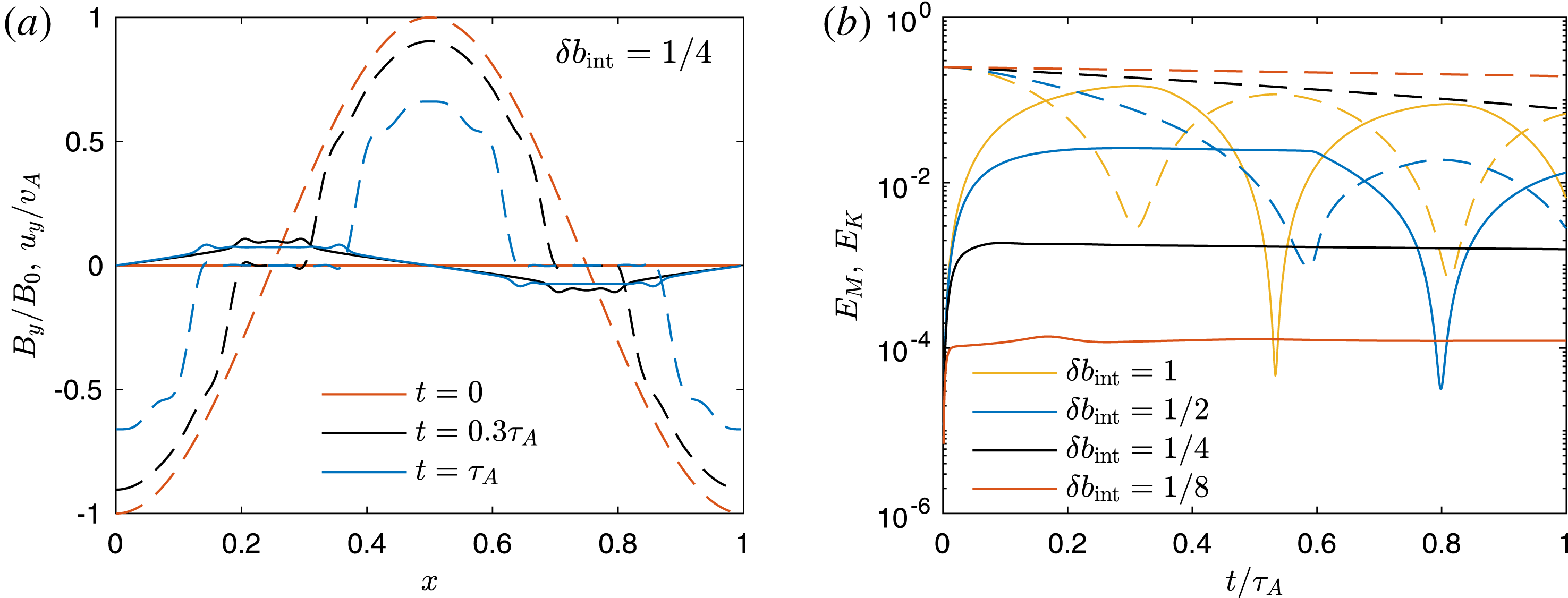
). In figure 1, we show some examples of wave interruption in the weakly collisional Braginskii MHD model (see § 2.2) at parameters chosen to match those of the turbulence simulations presented in § 3 (
 $\unicode[STIX]{x1D6FF}b_{\text{int}}$
from
 $1/8$
to 1, with initial perturbation amplitudes
 $\unicode[STIX]{x1D6FF}B_{\bot }/B_{0}=1$
). Note that for propagating or standing circularly polarized shear Alfvén waves, the magnetic field remains constant in time, so the interruption limit does not apply.
Interruption of linearly polarized shear Alfvén waves in the Braginskii MHD model, which is used for the turbulence simulations presented in § 3. Here we show results from simulations in one dimension, starting from a perpendicular magnetic perturbation
 $\unicode[STIX]{x1D6FF}B_{\bot }/B_{0}=1$
[
 $B_{y}=-B_{0}\cos (2\unicode[STIX]{x03C0}x)$
] with background magnetic field
 $\boldsymbol{B}_{0}=B_{0}\hat{\boldsymbol{x}}$
. In standard MHD, these initial conditions lead to standing-wave oscillations with period
 $\unicode[STIX]{x1D70F}_{A}$
. (a) Snapshots of the perpendicular velocity
 $u_{y}(x)/v_{A}$
(solid lines) and perpendicular magnetic field
 $B_{y}(x)/B_{0}$
(dashed lines) for
 $\unicode[STIX]{x1D6FF}b_{\text{int}}=1/4$
(Braginskii viscosity
 $\unicode[STIX]{x1D707}_{\text{Brag}}\equiv \unicode[STIX]{x1D708}_{c}^{-1}p_{0}=6$
; see § 2.2). We show snapshots at
 $t=0$
(red lines),
 $t=0.3\unicode[STIX]{x1D70F}_{A}$
(black lines) and
 $t=\unicode[STIX]{x1D70F}_{A}$
(blue lines). (b) Time evolution of kinetic energy (
 $E_{K}$
, solid lines) and magnetic energy (
 $E_{M}$
, dashed lines) at different
 $\unicode[STIX]{x1D6FF}b_{\text{int}}$
as labelled, from
 $\unicode[STIX]{x1D6FF}b_{\text{int}}=1$
to
 $\unicode[STIX]{x1D6FF}b_{\text{int}}=1/8$
(the black curves show the full time evolution of the wave in a). When the Braginskii viscosity is sufficiently large so that
 $\unicode[STIX]{x1D6FF}B_{\bot }/B_{0}\gtrsim \unicode[STIX]{x1D6FF}b_{\text{int}}$
, the system no longer supports shear Alfvénic oscillations; perturbations simply decay with
 $E_{M}\gg E_{K}$
until they can oscillate freely at amplitudes below
 $\unicode[STIX]{x1D6FF}b_{\text{int}}$
.

Our study here is designed to examine the influence of wave interruption on Alfvénic turbulence. The now-standard ‘critical balance’ paradigm (Goldreich & Sridhar Reference Goldreich and Sridhar1995, Reference Goldreich and Sridhar1997) posits that linear (shear-Alfvén-wave) and nonlinear time scales are comparable at all spatial scales in MHD turbulence. An immediate corollary is that if wave time scales are significantly modified due to wave interruption (which can occur at low amplitudes for
 $\unicode[STIX]{x1D6FD}\gg 1$
), then the turbulent cascade should also be strongly modified. Further, in the weakly collisional regime,
 $\unicode[STIX]{x1D6FF}b_{\text{int}}\propto \unicode[STIX]{x1D714}_{A}^{-1/2}\propto k_{\Vert }^{-1/2}$
has the same scaling as critically balanced fluctuations (
 $\unicode[STIX]{x1D6FF}u_{\bot }\propto k_{\Vert }^{-1/2}$
), suggesting that interruption effects should be important at all scales if they are important at the outer scale. Alternatively, one could state that, for outer-scale fluctuation amplitudes
 $\unicode[STIX]{x1D6FF}u_{\bot }/v_{A}\sim \unicode[STIX]{x1D6FF}B_{\bot }/B_{0}\gtrsim \unicode[STIX]{x1D6FF}b_{\text{int}}$
, pressure anisotropy is expected to be a stronger nonlinearity than the usual MHD nonlinearities across all scales of the turbulent cascade. This nonlinearity inhibits the oscillation of Alfvénic fluctuations (see figure 1), which seems to suggest that turbulence may not be possible for fluctuation amplitudes that exceed the interruption limit. This prediction is borne out in one dimension: stochastically driving linearly polarized shear Alfvén waves, one finds that the amplitude of velocity fluctuations is limited by (1.2). Likewise, in figure 1, we see that the kinetic energy of decaying shear Alfvénic perturbations is very small for
 $\unicode[STIX]{x1D6FF}b_{\text{int}}\lesssim 1/2$
. However, we will show in what follows that three-dimensional turbulence changes its characteristics to avoid this scenario, becoming ‘magneto-immutable’, while still supporting a turbulent cascade.
2 Magneto-immutable Alfvénic turbulence
Our starting point is the set of MHD equations with a pressure-anisotropy stress in the momentum equation:
 $$\begin{eqnarray}\displaystyle & \displaystyle \unicode[STIX]{x1D70C}\frac{\text{D}}{\text{D}t}\boldsymbol{u}=-\unicode[STIX]{x1D735}\left(p_{\bot }+\frac{B^{2}}{8\unicode[STIX]{x03C0}}\right)+\frac{1}{4\unicode[STIX]{x03C0}}\boldsymbol{B}\boldsymbol{\cdot }\unicode[STIX]{x1D735}\boldsymbol{B}+\unicode[STIX]{x1D735}\boldsymbol{\cdot }(\hat{\boldsymbol{b}}\hat{\boldsymbol{b}}\unicode[STIX]{x0394}p), & \displaystyle\end{eqnarray}$$
 $$\begin{eqnarray}\displaystyle & \displaystyle \frac{\text{D}}{\text{D}t}\boldsymbol{B}=\boldsymbol{B}\boldsymbol{\cdot }\unicode[STIX]{x1D735}\boldsymbol{u}-\boldsymbol{B}\unicode[STIX]{x1D735}\boldsymbol{\cdot }\boldsymbol{u}, & \displaystyle\end{eqnarray}$$
 $$\begin{eqnarray}\displaystyle & \displaystyle \frac{\text{D}}{\text{D}t}\unicode[STIX]{x0394}p=(p_{\bot }+2p_{\Vert })\hat{\boldsymbol{b}}\hat{\boldsymbol{b}}\boldsymbol{ : }\unicode[STIX]{x1D735}\boldsymbol{u}+(p_{\Vert }-2p_{\bot })\unicode[STIX]{x1D735}\boldsymbol{\cdot }\boldsymbol{u}+{\mathcal{Q}}(q_{\bot },q_{\Vert })-3\unicode[STIX]{x1D708}_{c}\unicode[STIX]{x0394}p. & \displaystyle\end{eqnarray}$$
Here
 $\unicode[STIX]{x1D70C}$
is the mass density,
 $\boldsymbol{u}$
is the flow velocity,
 $\boldsymbol{B}$
is the magnetic field,
 $\text{D}/\text{D}t\equiv \unicode[STIX]{x2202}/\unicode[STIX]{x2202}t+\boldsymbol{u}\boldsymbol{\cdot }\unicode[STIX]{x1D735}$
is the convective derivative and
 ${\mathcal{Q}}(q_{\bot },q_{\Vert })$
parameterizes the effects of heat fluxes (see, e.g. Chew et al.
Reference Chew, Goldberger and Low1956, Snyder, Hammett & Dorland Reference Snyder, Hammett and Dorland1997, Sulem & Passot Reference Sulem and Passot2015, Squire et al.
Reference Squire, Schekochihin and Quataert2017b
for explicit reference to the equations for
 $p_{\bot }$
and
 $p_{\Vert }$
individually, and for discussion of
 ${\mathcal{Q}}(q_{\bot },q_{\Vert })$
). The Alfvén speed is
 $v_{A}\equiv B/\sqrt{4\unicode[STIX]{x03C0}\unicode[STIX]{x1D70C}}$
. Throughout this work, we consider only subsonic dynamics with
 $\unicode[STIX]{x1D735}\boldsymbol{\cdot }\boldsymbol{u}\approx 0$
. Equations (2.1)–(2.3) may be derived directly from the kinetic equations (Kulsrud Reference Kulsrud, Sagdeev and Rosenbluth1983; Schekochihin et al.
Reference Schekochihin, Cowley, Rincon and Rosin2010) by assuming collisional (or cold) electrons and using the gyrotropy of the ion distribution on scales much larger than the gyroradius. They provide the simplest well-justified model for plasma dynamics on scales much larger than
 $\unicode[STIX]{x1D70C}_{i}$
.
2.1 Magneto-immutability and incompressibility
Although a complete solution to (2.1)–(2.3) requires specifying
 ${\mathcal{Q}}(q_{\bot },q_{\Vert })$
with a kinetic solution or closure, let us proceed for the moment without doing so. We draw analogies between the pressure-anisotropy force and the more familiar
 $\unicode[STIX]{x1D735}p$
force. In all fluid-like equations of state, pressure is coupled to flow divergences: it increases in compressions (
 $\unicode[STIX]{x1D735}\boldsymbol{\cdot }\boldsymbol{u}=\unicode[STIX]{x1D6FF}_{rs}\unicode[STIX]{x1D735}_{s}u_{r}=-\text{D}\ln \unicode[STIX]{x1D70C}/\text{D}t<0$
) and decreases in rarefactions (
 $\unicode[STIX]{x1D735}\boldsymbol{\cdot }\boldsymbol{u}>0$
). The pressure force (
 $-\unicode[STIX]{x1D735}p$
) isotropically drives the flow away from regions of large
 $p$
, thus pushing fluid away from compressions and towards rarefactions. This naturally leads to incompressibility, when pressure forces dominate over others in the system, rapidly eliminating compressional motions.
Similar ideas apply to pressure anisotropy and magneto-immutability. From (2.3), we see that pressure anisotropy is driven by ‘magneto-dilations’, where
 $\hat{\boldsymbol{b}}\hat{\boldsymbol{b}}\boldsymbol{ : }\unicode[STIX]{x1D735}\boldsymbol{u}=\hat{b}_{s}\hat{b}_{r}\unicode[STIX]{x1D735}_{s}u_{r}=\text{D}\ln B/\text{D}t+\unicode[STIX]{x1D735}\boldsymbol{\cdot }\boldsymbol{u}\neq 0$
. The pressure-anisotropy stress in (2.1) has the form
 $\unicode[STIX]{x1D735}\boldsymbol{\cdot }(\hat{\boldsymbol{b}}\hat{\boldsymbol{b}}\unicode[STIX]{x0394}p)=\unicode[STIX]{x1D735}_{r}(\hat{b}_{i}\hat{b}_{r}\unicode[STIX]{x0394}p)$
, and is akin to an anisotropic version of
 $-\unicode[STIX]{x1D735}p=-\unicode[STIX]{x1D735}_{r}(\unicode[STIX]{x1D6FF}_{\text{ir}}p)$
: it is a force that acts in a direction nearly aligned with
 $\hat{\boldsymbol{b}}$
(so long as
 $\hat{\boldsymbol{b}}$
does not vary significantly in space), and arises due to variations in
 $\unicode[STIX]{x0394}p$
along the
 $\hat{\boldsymbol{b}}$
direction.Footnote
1
We thus expect that the pressure-anisotropy stress will drive field-aligned flows that minimize
 $\hat{\boldsymbol{b}}\hat{\boldsymbol{b}}\boldsymbol{ : }\unicode[STIX]{x1D735}\boldsymbol{u}\approx \text{D}\ln B/\text{D}t$
. Such a flow will resist changes in the magnetic-field strength; i.e. it will approach ‘magneto-immutability’.
Note that there is no requirement that incompressibility and magneto-immutability act separately. Indeed, for trans-Alfvénic (
 $\unicode[STIX]{x1D6FF}B_{\bot }\sim B$
) turbulence in a collisionless plasma, both effects can be of the same order. In this case, it will be important to consider the combined impact of compressions and magneto-dilations, as opposed to each separately, and there may be interesting self-organization principles that apply to combinations of
 $B$
and
 $\unicode[STIX]{x1D70C}$
. However, in this work, our focus on the weakly collisional model implies that magneto-immutability is subdominant to incompressibility (see next section). We thus consider the two effects separately, leaving speculation about their interaction in collisionless plasma turbulence to future work.
2.2 Alfvénic turbulence with Braginskii viscosity
Although the arguments in the preceding paragraphs are quite general, we focus here on applying them to strong, Alfvénic turbulence (Goldreich & Sridhar Reference Goldreich and Sridhar1995) in the weakly collisional limit. We define the turbulence amplitude
 $\unicode[STIX]{x1D6FF}b_{\text{turb}}\equiv \unicode[STIX]{x1D6FF}B_{\bot }/B_{0}\sim \unicode[STIX]{x1D6FF}u_{\bot }/v_{A}$
and the Alfvén frequency
 $\unicode[STIX]{x1D714}_{A}=k_{\Vert }v_{A}$
(where
 $k_{\Vert }^{-1}\sim l_{\Vert }$
is the field-parallel scale of a given fluctuation, and
 $k_{\bot }^{-1}$
is its perpendicular scale). We assume that
 $\unicode[STIX]{x1D6FD}\gg \unicode[STIX]{x1D708}_{c}/\unicode[STIX]{x1D714}_{A}\gg \unicode[STIX]{x1D6FD}^{1/2}\gg 1$
(or, equivalently,
 $\unicode[STIX]{x1D6FD}^{-1/2}\ll k_{\Vert }\unicode[STIX]{x1D706}_{\text{mfp}}\ll 1$
), so that the ion-collision time scale
 $\unicode[STIX]{x1D708}_{c}^{-1}$
is longer than all other time scales, including those associated with
 ${\mathcal{Q}}(q_{\bot },q_{\Vert })$
(Mikhailovskii & Tsypin Reference Mikhailovskii and Tsypin1971; Squire et al.
Reference Squire, Schekochihin and Quataert2017b
). The result is a closure for
 $\unicode[STIX]{x0394}p$
in which
 $\unicode[STIX]{x0394}p$
is smaller than the variation in
 $p_{\bot }$
or
 $p_{\Vert }$
individually. Equation (2.3) becomes
 $$\begin{eqnarray}\unicode[STIX]{x0394}p\approx \frac{p_{0}}{\unicode[STIX]{x1D708}_{c}}\hat{\boldsymbol{b}}\hat{\boldsymbol{b}}\boldsymbol{ : }\unicode[STIX]{x1D735}\boldsymbol{u},\end{eqnarray}$$
where
 $\unicode[STIX]{x0394}p\ll p_{\bot }\simeq p_{\Vert }\simeq p_{0}$
(Braginskii Reference Braginskii1965). Because
 $\unicode[STIX]{x1D6FD}\gg 1$
, the flow is nearly incompressible and
 $p_{0}\simeq \text{const}.$
in (2.4). The pressure-anisotropy stress then takes the form of a field-aligned viscous stress
 $\unicode[STIX]{x1D707}_{\text{Brag}}\unicode[STIX]{x1D735}\boldsymbol{\cdot }[\hat{\boldsymbol{b}}\hat{\boldsymbol{b}}(\hat{\boldsymbol{b}}\hat{\boldsymbol{b}}\boldsymbol{ : }\unicode[STIX]{x1D735}\boldsymbol{u})]$
, where
 $\unicode[STIX]{x1D707}_{\text{Brag}}\equiv \unicode[STIX]{x1D708}_{c}^{-1}p_{0}$
is the Braginskii viscosity. This model is thus often called ‘Braginskii MHD’. As discussed in § 1.1, intuitively, we expect a strong modification of the turbulence for amplitudes above which shear Alfvén waves are interrupted and cannot propagate:
 $\unicode[STIX]{x1D6FF}b_{\text{turb}}\gtrsim \unicode[STIX]{x1D6FF}b_{\text{int}}\equiv 2\unicode[STIX]{x1D6FD}^{-1/2}\sqrt{\unicode[STIX]{x1D708}_{c}/\unicode[STIX]{x1D714}_{A}}$
. Note that, because
 $\unicode[STIX]{x1D708}_{c}\gg \unicode[STIX]{x1D714}_{A}$
, a weakly collisional plasma with fluctuations that satisfy
 $\unicode[STIX]{x1D6FF}b_{\text{turb}}\gtrsim \unicode[STIX]{x1D6FF}b_{\text{int}}$
necessarily also has
 $\unicode[STIX]{x1D6FD}\gg 1$
, justifying our use of an incompressible model in § 3 below.
Because
 $\unicode[STIX]{x0394}p\propto \hat{\boldsymbol{b}}\hat{\boldsymbol{b}}\boldsymbol{ : }\unicode[STIX]{x1D735}\boldsymbol{u}$
, the Braginskii viscous stress acts in the direction required to make the flow magneto-immutable. The fact that it irreversibly dissipates kinetic energy (unlike, for example, the pressure force
 $-\unicode[STIX]{x1D735}p$
) is not important for our arguments here. A direct analogy for compressional motions is the bulk viscosity, which has the form
 $-\unicode[STIX]{x1D707}_{\text{bulk}}\unicode[STIX]{x1D735}(\unicode[STIX]{x1D735}\boldsymbol{\cdot }\boldsymbol{u})$
and damps compression and rarefaction of the flow. Interestingly, flows with large bulk viscosities (which are not commonly studied) are effectively incompressible even when the Mach number based on the thermal pressure is large (Pan & Johnsen Reference Pan and Johnsen2017).
By analogy with the Reynolds number – which is the ratio of viscous to inertial time scales, viz.,
 $Re=\unicode[STIX]{x1D70C}\unicode[STIX]{x1D6FF}u_{\bot }l_{\bot }/\unicode[STIX]{x1D707}_{\text{iso}}\sim \unicode[STIX]{x1D70C}v_{A}l_{\Vert }/\unicode[STIX]{x1D707}_{\text{iso}}$
in MHD turbulence (with isotropic dynamic viscosity
 $\unicode[STIX]{x1D707}_{\text{iso}}$
) – we define the Braginskii ‘interruption number’
 $\text{It}_{\text{Brag}}$
.
 $\text{It}_{\text{Brag}}$
is the ratio of the time scale for the parallel viscous stress to act on an Alfvénically polarized motion,Footnote
2
 $t_{\text{int}}\sim \unicode[STIX]{x1D714}_{A}^{-1}\unicode[STIX]{x1D6FF}b_{\text{int}}^{2}/\unicode[STIX]{x1D6FF}b_{\text{turb}}^{2}$
(see Squire et al.
Reference Squire, Schekochihin and Quataert2017b
), and the inertial time scale,
 $t_{\text{inertial}}\sim (k_{\bot }\unicode[STIX]{x1D6FF}u_{\bot })^{-1}\sim (k_{\Vert }v_{A})^{-1}$
(assuming critically balanced turbulence; Goldreich & Sridhar Reference Goldreich and Sridhar1995, Reference Goldreich and Sridhar1997), giving
 $$\begin{eqnarray}\text{It}_{\text{Brag}}\equiv \frac{t_{\text{int}}}{t_{\text{inertial}}}\approx \frac{\unicode[STIX]{x1D6FF}b_{\text{int}}^{2}}{\unicode[STIX]{x1D6FF}b_{\text{turb}}^{2}}\sim \frac{\unicode[STIX]{x1D70C}v_{A}l_{\Vert }}{\unicode[STIX]{x1D707}_{\text{Brag}}}\left(\frac{\unicode[STIX]{x1D6FF}B_{\bot }^{2}}{B_{0}^{2}}\right)^{-1}.\end{eqnarray}$$
The Braginskii stress will be dynamically important, i.e. comparable to the Maxwell and Reynolds stresses,
 $\boldsymbol{B}\boldsymbol{\cdot }\unicode[STIX]{x1D735}\boldsymbol{B}$
and
 $\boldsymbol{u}\boldsymbol{\cdot }\unicode[STIX]{x1D735}\boldsymbol{u}$
, for
 $\text{It}_{\text{Brag}}\lesssim 1$
, or equivalently
 $\unicode[STIX]{x1D6FF}b_{\text{turb}}\gtrsim \unicode[STIX]{x1D6FF}b_{\text{int}}$
. As discussed above, when
 $\unicode[STIX]{x1D707}_{\text{Brag}}$
is so large that
 $\text{It}_{\text{Brag}}\lesssim 1$
, motions become increasingly magneto-immutable, limiting
 $\unicode[STIX]{x0394}p$
fluctuations to
 $\unicode[STIX]{x0394}p\sim B^{2}$
, in order to balance
 $\boldsymbol{B}\boldsymbol{\cdot }\unicode[STIX]{x1D735}\boldsymbol{B}$
. Thus, when
 $\text{It}_{\text{Brag}}\ll 1$
, keeping the amplitudes of
 $\boldsymbol{u}$
and
 $\boldsymbol{B}$
fluctuations approximately constant and changing
 $\unicode[STIX]{x1D707}_{\text{Brag}}$
, we expect
 $(\hat{\boldsymbol{b}}\hat{\boldsymbol{b}}\boldsymbol{ : }\unicode[STIX]{x1D735}\boldsymbol{u})_{\text{rms}}\propto \text{It}_{\text{Brag}}$
, or
 $\unicode[STIX]{x0394}p_{\text{rms}}\sim \text{const}.$
, as opposed to the naive scaling,
 $(\hat{\boldsymbol{b}}\hat{\boldsymbol{b}}\boldsymbol{ : }\unicode[STIX]{x1D735}\boldsymbol{u})_{\text{rms}}\sim \text{const}.$
, or
 $\unicode[STIX]{x0394}p_{\text{rms}}\propto \text{It}_{\text{Brag}}^{-1}$
, which holds at
 $\text{It}_{\text{Brag}}\gg 1$
when pressure-anisotropy forces play no role (here,
 $A_{\text{rms}}$
denotes the root-mean-squared fluctuation level of the variable
 $A$
). Note that in realistic plasmas, where microinstabilities can break the direct proportionality between
 $\hat{\boldsymbol{b}}\hat{\boldsymbol{b}}\boldsymbol{ : }\unicode[STIX]{x1D735}\boldsymbol{u}$
and
 $\unicode[STIX]{x0394}p$
(see § 2.3 below), these scalings hold only in regions that are not affected by microinstabilities.Footnote
3
2.3 Microinstabilities
Sufficiently non-Maxwellian distribution functions are unstable to kinetic plasma instabilities, complicating the arguments above and breaking the correspondence between compression/rarefaction and magneto-dilation. In the high-
 $\unicode[STIX]{x1D6FD}$
regime, the most relevant microinstabilities are the firehose (Rosenbluth Reference Rosenbluth1956) and mirror (Barnes Reference Barnes1966; Hasegawa Reference Hasegawa1969), which are triggered when
 $\unicode[STIX]{x0394}p\lesssim -B^{2}/4\unicode[STIX]{x03C0}$
and
 $\unicode[STIX]{x0394}p\gtrsim B^{2}/8\unicode[STIX]{x03C0}$
, respectively. These instabilities act to deplete the amount of large-scale
 $\unicode[STIX]{x0394}p$
in excess of the stability thresholds (
 $|\unicode[STIX]{x0394}p|\lesssim B^{2}/4\unicode[STIX]{x03C0}$
; Hellinger & Trávníček Reference Hellinger and Trávníček2008; Schekochihin et al.
Reference Schekochihin, Cowley, Kulsrud, Rosin and Heinemann2008; Kunz, Schekochihin & Stone Reference Kunz, Schekochihin and Stone2014; Melville, Schekochihin & Kunz Reference Melville, Schekochihin and Kunz2016), which they achieve over short time scales set by
 $\unicode[STIX]{x1D6FA}_{i}$
. They may thus frustrate the plasma’s attempts to become magneto-immutable by truncating the growth of
 $\unicode[STIX]{x0394}p$
when it becomes too large. There is no analogue to this effect in (collisional) compressible hydrodynamic flows, which are generally not strongly affected by kinetic instabilities because large variations in isotropic pressure can occur even when
 $\unicode[STIX]{x1D708}_{c}^{-1}$
is small compared to all other time scales (unlike
 $\unicode[STIX]{x0394}p$
, which is always negligibly small at sufficiently small
 $\unicode[STIX]{x1D708}_{c}^{-1}$
). Nonetheless, we argue, and show explicitly below (figure 4), that magneto-immutability remains an important self-organizing principle, even if mirror and firehose perfectly limit
 $\unicode[STIX]{x0394}p$
(i.e.
 $-B^{2}/4\unicode[STIX]{x03C0}\leqslant \unicode[STIX]{x0394}p\leqslant B^{2}/8\unicode[STIX]{x03C0}$
). The reason is that the two effects, microinstabilities and magneto-immutability, scale in identical ways: they are both important only once
 $\unicode[STIX]{x0394}p\sim B^{2}$
, implying that the limiting effect of microinstabilities does not dominate over magneto-immutability, or vice versa.
3 Braginskii MHD simulations
We now supplement the heuristic arguments proposed above by numerical simulations of Alfvénic turbulence. We use incompressible Braginskii MHD ((2.1)–(2.2) with
 $\unicode[STIX]{x0394}p$
given by (2.4)) because it is the simplest model that captures the pressure-anisotropy effects of interest, allowing comparatively straightforward diagnosis of the key physics. The results of these simulations demonstrate three key points: (i) that magneto-immutable turbulence with
 $\text{It}_{\text{Brag}}\lesssim 1$
(
 $\unicode[STIX]{x1D6FF}b_{\text{turb}}\gtrsim \unicode[STIX]{x1D6FF}b_{\text{int}}$
) is possible and similar to standard critically balanced Alfvénic MHD turbulence (although some key differences do exist); (ii) that the pressure-anisotropy stress does indeed act to minimize
 $\hat{\boldsymbol{b}}\hat{\boldsymbol{b}}\boldsymbol{ : }\unicode[STIX]{x1D735}\boldsymbol{u}$
; and (iii) that the system approaches a well-defined non-zero turbulent state in the
 $\text{It}_{\text{Brag}}\rightarrow 0$
limit, similarly to the way in which hydrodynamic turbulence approaches incompressibility in the low-Mach-number limit.
3.1 Numerics
Our simulations use the Snoopy code (Lesur & Longaretti Reference Lesur and Longaretti2007), which is based on a Fourier pseudo-spectral discretization in space. The pressure anisotropy
 $\unicode[STIX]{x0394}p$
is calculated from (2.4), with sub-cycling of the final term in (2.1) eight times per global MHD time step. The effect of microinstabilities is modelled by limiting the value of
 $\unicode[STIX]{x0394}p$
(Sharma et al.
Reference Sharma, Hammett, Quataert and Stone2006), viz.,
 $\unicode[STIX]{x0394}p=\min (\unicode[STIX]{x1D707}_{\text{Brag}}\hat{\boldsymbol{b}}\hat{\boldsymbol{b}}\boldsymbol{ : }\unicode[STIX]{x1D735}\boldsymbol{u},B^{2}/8\unicode[STIX]{x03C0})$
(mirror) or
 $\unicode[STIX]{x0394}p=\max (\unicode[STIX]{x1D707}_{\text{Brag}}\hat{\boldsymbol{b}}\hat{\boldsymbol{b}}\boldsymbol{ : }\unicode[STIX]{x1D735}\boldsymbol{u},-B^{2}/4\unicode[STIX]{x03C0})$
(firehose). Because the parallel firehose instability is captured by the Braginskii MHD model but the mirror instability is not, most simulations use only a mirror limiter. This choice also helps us to isolate the effects of magneto-immutability from those of the limiter, because
 $\unicode[STIX]{x0394}p$
freely evolves in regions where
 $\unicode[STIX]{x0394}p<0$
. However, we acknowledge that some crucial aspects of the true kinetic firehose instability – in particular, pitch-angle scattering of particles from ion-Larmor-scale fluctuations – are not captured by Braginskii MHD. For this reason, we also run some turbulence simulations with both a mirror and a firehose limiter, which show similar qualitative behaviours to those with just a mirror limiter. We use periodic boundary conditions in a three-dimensional box threaded by a uniform mean magnetic field
 $\boldsymbol{B}_{0}=B_{0}\hat{\boldsymbol{x}}$
. In all cases,
 $L_{y}/L_{z}=1$
, whereas
 $L_{x}/L_{z}$
is varied depending upon the amplitude of the turbulent fluctuations. The latter are driven by forcing all modes of the velocity field up to (
 $|k_{x}|=2\times 2\unicode[STIX]{x03C0}/L_{x}$
,
 $|k_{y}|=2\times 2\unicode[STIX]{x03C0}/L_{y}$
,
 $|k_{z}|=2\times 2\unicode[STIX]{x03C0}/L_{z}$
) using an Orstein–Uhlenbeck process with correlation time
 ${\sim}\unicode[STIX]{x1D70F}_{A}\equiv L_{x}/v_{A}$
. The amplitude of the driving is chosen such that
 $\unicode[STIX]{x1D6FF}b_{\text{turb}}\equiv \unicode[STIX]{x1D6FF}B_{\bot }/B_{0}\sim \unicode[STIX]{x1D6FF}u_{\bot }/v_{A}\sim L_{y}/L_{x}=L_{z}/L_{x}$
; i.e. we drive turbulence in critical balance,
 $k_{\Vert }v_{A}\sim k_{\bot }u_{\bot }$
(Goldreich & Sridhar Reference Goldreich and Sridhar1995). We present results for both trans-Alfvénic turbulence, with
 $L_{x}=L_{z}$
(
 $\unicode[STIX]{x1D6FF}b_{\text{turb}}\approx 1$
), and sub-Alfvénic turbulence in a box that is elongated along the mean-field direction, with
 $L_{x}=4L_{z}$
(
 $\unicode[STIX]{x1D6FF}b_{\text{turb}}\approx 1/4$
). We use fourth-order isotropic hyper-dissipation in
 $\boldsymbol{u}$
and
 $\boldsymbol{B}$
(
 $\unicode[STIX]{x1D707}_{\text{iso},4}\unicode[STIX]{x1D6FB}^{4}\boldsymbol{u}$
and
 $\unicode[STIX]{x1D702}_{4}\unicode[STIX]{x1D6FB}^{4}\boldsymbol{B}$
), which was chosen, after extensive testing with MHD simulations, because it gave the cleanest inertial range at a given resolution. Simulations are run until
 $t=4\unicode[STIX]{x1D70F}_{A}$
and results are averaged over the final
 $2\unicode[STIX]{x1D70F}_{A}$
.
We change the relative importance of the pressure-anisotropy stress by varying
 $\unicode[STIX]{x1D707}_{\text{Brag}}$
at constant forcing amplitude and constant
 $B_{0}$
. As explained in § 2, we expect pressure anisotropy to be important when
 $\text{It}_{\text{Brag}}\lesssim 1$
, or equivalently for
 $\unicode[STIX]{x1D707}_{\text{Brag}}\gtrsim \unicode[STIX]{x03C0}^{-1}\unicode[STIX]{x1D70C}v_{A}L_{x}^{3}/L_{z}^{2}$
(see (2.5)). Unfortunately, such a large
 $\unicode[STIX]{x1D707}_{\text{Brag}}$
requires very short time steps. Consequently, simulations at small
 $\text{It}_{\text{Brag}}$
are vastly more expensive computationally than their MHD counterparts, and our highest resolutions are rather modest:
 $N_{x}=N_{y}=N_{z}=N_{x,y,z}=192$
. Although other numerical methods may enable increased resolution in future work, great care must be taken: due to the large values of
 $\unicode[STIX]{x1D707}_{\text{Brag}}$
, very small errors in evaluating
 $\hat{\boldsymbol{b}}\hat{\boldsymbol{b}}\boldsymbol{ : }\unicode[STIX]{x1D735}\boldsymbol{u}$
can spuriously damp legitimate motions. We chose the pseudo-spectral method after extensive tests of decaying turbulence with
 $\text{It}_{\text{Brag}}>1$
but large
 $\unicode[STIX]{x1D707}_{\text{Brag}}$
, using a variety of different numerical methods. In particular, unexpected problems arose in evaluating the Braginskii stress using finite-volume, operator-split methods.
3.2 Results
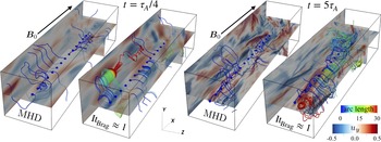
To illustrate a magneto-immutable flow, in figure 2 we compare the flow streamlines at early times using
 $\text{It}_{\text{Brag}}\approx 1$
Braginskii MHD with those obtained using standard MHD. Although the magnitude of the velocity in each case is similar, the magneto-immutable flow has manifestly different structure: plasma is constrained to flow along the direction that minimizes changes in
 $B$
. The dynamics illustrated in figure 2 may be thought of as a nonlinear generalization of a circularly polarized linear Alfvén wave, which does not change the strength of
 $B$
.
The effect of pressure-anisotropy stress on the flow structure. In each panel, the colour scale on each slice shows
 $u_{y}$
(perpendicular to
 $\boldsymbol{B}_{0}$
), while the lines follow the streamlines of the incompressible flow (the colour shows the length of a streamline from its origin, to more clearly show the different flow structures in each case). We compare MHD and
 $\text{It}_{\text{Brag}}=1$
flows, driven with identical forcing fields from zero initial conditions. The pair of panels on the left is for
 $t=\unicode[STIX]{x1D70F}_{A}/4=0.25L_{x}/v_{A}$
, at which point the flow has not yet become fully turbulent, while the panels on the right show turbulent flow structures at
 $t=5\unicode[STIX]{x1D70F}_{A}=5L_{x}/v_{A}$
. In both cases, the effect of magneto-immutability is clearly seen in the flow lines, which become more tightly curled so that the flow has the direction required to avoid changes in
 $B$
. This is a nonlinear analogue of a circularly polarized Alfvén wave.

We now describe the key findings of our turbulence simulations (illustrated in figures 3–6) and how these add to the discussion of § 2.
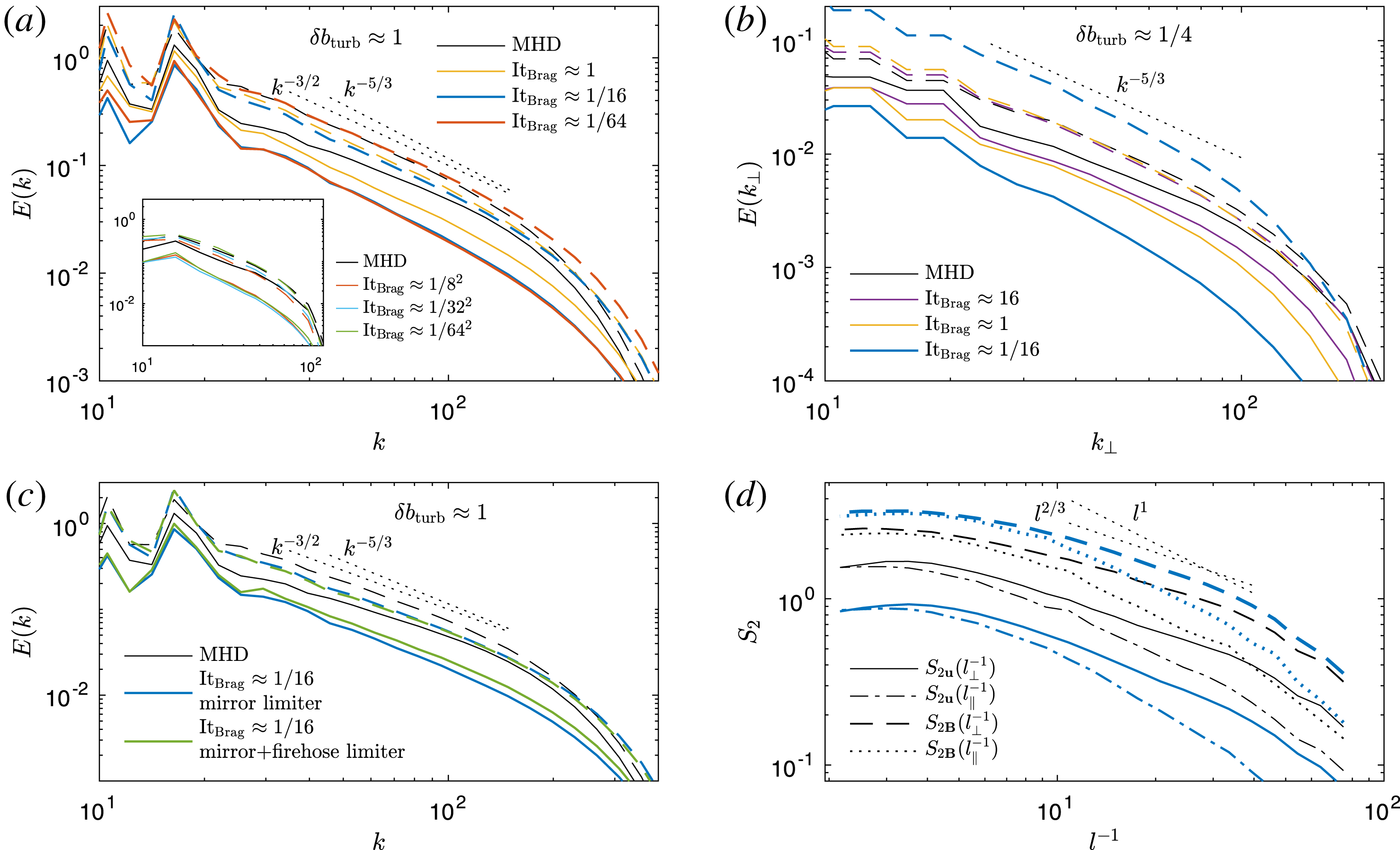
(a) Kinetic-energy (
 $E_{K}$
, solid lines) and magnetic-energy (
 $E_{M}$
, dashed lines) spectra, for trans-Alfvénic turbulence simulations with
 $\unicode[STIX]{x1D6FF}b_{\text{turb}}=\unicode[STIX]{x1D6FF}B_{\bot }/B_{0}\approx 1$
(
 $L_{x}=1$
) at resolution
 $N_{x,y,z}=192$
, and a mirror limiter but no firehose limiter. As labelled, the different colours show simulations with different
 $\text{It}_{\text{Brag}}\approx \unicode[STIX]{x1D6FF}b_{\text{int}}^{2}/\unicode[STIX]{x1D6FF}b_{\text{turb}}^{2}$
. We expect the turbulence to be affected by magneto-immutability for
 $\text{It}_{\text{Brag}}\lesssim 1$
. The inset shows spectra for low-resolution simulations (
 $N_{x,y,z}=48$
) at even smaller
 $\text{It}_{\text{Brag}}$
. (b) Spectra for sub-Alfvénic-turbulence simulations,
 $\unicode[STIX]{x1D6FF}b_{\text{turb}}=\unicode[STIX]{x1D6FF}B_{\bot }/B_{0}=1/4$
(
 $L_{x}=4$
) and resolution
 $N_{x,y,z}=96$
(we bin energies in
 $k_{\bot }=(k_{y}^{2}+k_{z}^{2})^{1/2}$
in this case due to the elongated box). (c) As in (a) (trans-Alfvénic turbulence,
 $L_{x}=1$
), but comparing the case with only a mirror limiter (blue) to that with both a mirror and firehose limiter (green) for
 $\text{It}_{\text{Brag}}\approx 1/16$
. The two are very similar, with a slightly smaller residual energy when the firehose limiter is used. (d) Anisotropic structure functions of the magnetic and kinetic energy (
 $S_{2\boldsymbol{B}}=\langle [\boldsymbol{B}(\boldsymbol{x}+\boldsymbol{l})-\boldsymbol{B}(\boldsymbol{x})]^{2}\rangle$
and
 $S_{2\boldsymbol{u}}=\langle [\boldsymbol{u}(\boldsymbol{x}+\boldsymbol{l})-\boldsymbol{u}(\boldsymbol{x})]^{2}\rangle$
, respectively) for trans-Alfvénic turbulence (
 $L_{x}=1$
). Blue curves show
 $\text{It}_{\text{Brag}}\approx 1/16$
Braginskii MHD turbulence while black curves show MHD (we plot
 $S_{2}$
versus
 $l^{-1}$
for comparison with the other panels). The increments
 $\boldsymbol{l}$
are taken either perpendicular to the local scale-dependent magnetic field,
 $S_{2}(l_{\bot }^{-1})$
, or parallel to the field,
 $S_{2}(l_{\Vert }^{-1})$
, illustrating increasing anisotropy at small scales, as in MHD (Goldreich & Sridhar Reference Goldreich and Sridhar1995, Reference Goldreich and Sridhar1997).

3.2.1 Turbulence is possible and Alfvénic in character
As discussed in § 1.1, it is not obvious that turbulent motions can be supported at all when
 $\unicode[STIX]{x1D6FF}b_{\text{turb}}\gtrsim \unicode[STIX]{x1D6FF}b_{\text{int}}$
(
 $\text{It}_{\text{Brag}}\lesssim 1$
), because isolated linearly polarized Alfvénic fluctuations cannot propagate (even with mirror and/or firehose limiters; Squire et al.
Reference Squire, Quataert and Schekochihin2016). Our first result, illustrated in figure 3, is that Braginskii MHD can sustain turbulence when
 $\text{It}_{\text{Brag}}<1$
. Energy spectra are similar to those in MHD, but with increasing turbulent residual energy,
 $E_{R}\equiv [\langle (\boldsymbol{B}-\boldsymbol{B}_{0})^{2}\rangle -\langle \boldsymbol{u}^{2}\rangle ]/[\langle (\boldsymbol{B}-\boldsymbol{B}_{0})^{2}\rangle \langle \boldsymbol{u}^{2}\rangle ]^{1/2}$
, at low
 $\text{It}_{\text{Brag}}$
(i.e. the system becomes more magnetically dominated, as occurs in an interrupted shear Alfvén wave). Spectral slopes are close to
 $k^{-5/3}$
, or slightly shallower (cf. Maron & Goldreich Reference Maron and Goldreich2001; Boldyrev Reference Boldyrev2006; Beresnyak Reference Beresnyak2012; Perez et al.
Reference Perez, Mason, Boldyrev and Cattaneo2012). Comparing figures 3(a) and 3(b), we see that trans-Alfvénic and sub-Alfvénic turbulence are broadly similar at the same
 $\text{It}_{\text{Brag}}$
, viz.,
 $\unicode[STIX]{x1D6FF}b_{\text{int}}=1/4$
turbulence with
 $\unicode[STIX]{x1D6FF}b_{\text{turb}}\approx 1/4$
is comparable to
 $\unicode[STIX]{x1D6FF}b_{\text{int}}=1$
turbulence with
 $\unicode[STIX]{x1D6FF}b_{\text{turb}}\approx 1$
(although the residual energy is larger in the sub-Alfvénic case). We also see, in figure 3(c), that
 $\text{It}_{\text{Brag}}<1$
turbulence with both mirror and firehose limiters on
 $\unicode[STIX]{x0394}p$
is relatively similar to that with just a mirror limiter, aside from the slightly smaller
 $E_{R}$
.
We have run a variety of other common MHD-turbulence diagnostics on these simulation sets, including calculations of anisotropic structure functions of the kinetic and magnetic energy, which are shown in figure 3(d) for the trans-Alfvénic MHD and
 $\text{It}_{\text{Brag}}=1/16$
simulations. These are calculated using the method of Chen et al. (Reference Chen, Mallet, Yousef, Schekochihin and Horbury2011) and Mallet, Schekochihin & Chandran (Reference Mallet, Schekochihin and Chandran2015), by selecting for increments
 $\boldsymbol{l}$
that are either perpendicular (
 $\cos ^{-1}(\hat{\boldsymbol{l}}\boldsymbol{\cdot }\hat{\boldsymbol{b}})>70^{\circ }$
) or parallel (
 $\cos ^{-1}(\hat{\boldsymbol{l}}\boldsymbol{\cdot }\hat{\boldsymbol{b}})<20^{\circ }$
) to the local magnetic field around the chosen increment
 $\boldsymbol{B}[(\boldsymbol{x}_{1}+\boldsymbol{x}_{2})/2]$
, where
 $\boldsymbol{l}=\boldsymbol{x}_{2}-\boldsymbol{x}_{1}$
. We clearly see the signatures of scale-dependent anisotropy in both simulations, with the cascade following the scalings
 $S_{2}\sim l_{\bot }^{2/3}$
and
 $S_{2}\sim l_{\Vert }^{1}$
usually expected for a critically balanced MHD cascade. Note that this calculation is carried out on the trans-Alfvénic simulations in a cubic box with isotropic forcing, so the anisotropy measurement is not influenced by the assumption of critical balance in the outer-scale forcing. We have also computed the alignment of
 $\boldsymbol{u}$
and
 $\boldsymbol{B}$
(using the method of Mallet et al.
Reference Mallet, Schekochihin, Chandran, Chen, Horbury, Wicks and Greenan2016), again finding no striking differences compared to MHD turbulence (not shown).
Overall, the biggest difference compared to MHD is the increase in
 $E_{R}$
. This appears to be related, in part, to
 $\langle \unicode[STIX]{x0394}p\rangle$
being negative (thus changing the ratio of
 $\unicode[STIX]{x1D6FF}u_{\bot }$
to
 $\unicode[STIX]{x1D6FF}B_{\bot }$
in an Alfvén wave), as well as to the extra dissipation in the momentum equation (but not the induction equation) due to Braginskii viscosity (see figure 6
a). However, the behaviour of
 $E_{R}$
, including why its relative increase is larger in sub-Alfvénic than trans-Alfvénic turbulence, is not well understood by us at the present time. More generally, aside from these differences in
 $E_{R}$
, it remains unclear how
 $\text{It}_{\text{Brag}}<1$
turbulence can be so similar to MHD turbulence. The magnitude of the velocity fluctuations remains well above the interruption limit in all
 $\text{It}_{\text{Brag}}<1$
simulations (and for
 $\text{It}_{\text{Brag}}\ll 1$
, severely so), implying that isolated linearly polarized Alfvénic fluctuations would be unable to propagate for amplitudes similar to those we find in our turbulence (see § 1.1 for further discussion). Evidently, further study of other statistics and the structures in the flow and magnetic field is warranted (see, e.g. Perez & Boldyrev Reference Perez and Boldyrev2009; Zhdankin, Boldyrev & Uzdensky Reference Zhdankin, Boldyrev and Uzdensky2016). However, given the limited resolution of our simulations, we leave this to future work.
The spectra and structure functions shown in figure 3 are specific to Braginskii MHD with microinstability limiter(s). Although an exhaustive survey is not the purpose of this work, it is helpful to briefly comment on their robustness. Spectral slopes and general features (e.g. scale-dependent anisotropy) are robust to changing the mirror-limit threshold, although, like the addition of a firehose limit (figure 3
c), these modifications result in modest changes in the residual energy at a given
 $\text{It}_{\text{Brag}}$
. In the unphysical case without microinstability limiters – i.e. when
 $\unicode[STIX]{x0394}p$
is completely free to evolve – the characteristics of the turbulence differ further, because
 $\langle \unicode[STIX]{x0394}p\rangle$
is tied directly to the dissipation of
 $\boldsymbol{B}$
, thus driving
 $\langle \unicode[STIX]{x0394}p\rangle >0$
(see figure 4).Footnote
4
Finally, because
 $\unicode[STIX]{x1D6FF}b_{\text{int}}$
depends on
 $k_{\Vert }$
in the weakly collisional regime (through
 $\unicode[STIX]{x1D714}_{A}$
) but not in the collisionless regime (see (1.2)), these spectra are likely specific to Braginskii MHD. Further simulations are required to explore spectra in collisionless high-
 $\unicode[STIX]{x1D6FD}$
plasmas.
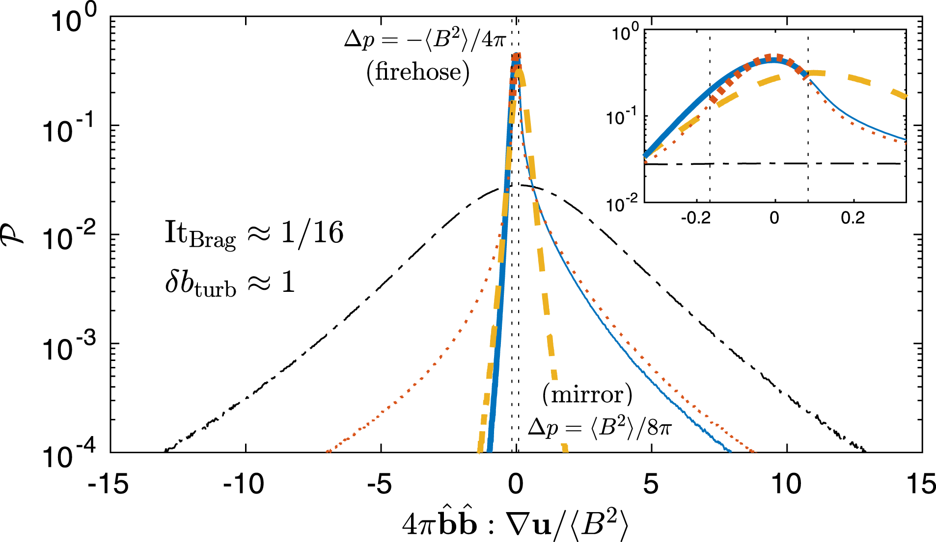
Probability density function (PDF) of
 $4\unicode[STIX]{x03C0}\hat{\boldsymbol{b}}\hat{\boldsymbol{b}}\boldsymbol{ : }\unicode[STIX]{x1D735}\boldsymbol{u}/\langle B^{2}\rangle$
for
 $\unicode[STIX]{x1D6FF}b_{\text{turb}}\approx 1$
(
 $L_{x}=1$
) simulations (spectra shown in figure 3). We compare MHD turbulence (black-dot-dashed line) to
 $\text{It}_{\text{Brag}}\approx 1/16$
(
 $\unicode[STIX]{x1D6FF}b_{\text{int}}\approx 1/4$
,
 $\unicode[STIX]{x1D707}_{\text{Brag}}\approx 2$
) turbulence with a mirror limiter (blue line), with both mirror and firehose limiters (red-dotted line), and with no limiters (yellow-dashed line). The vertical dotted lines denote the mirror and firehose limits for the
 $\text{It}_{\text{Brag}}\approx 1/16$
simulations. Regions with thicker lines (e.g.
 $\hat{\boldsymbol{b}}\hat{\boldsymbol{b}}\boldsymbol{ : }\unicode[STIX]{x1D735}\boldsymbol{u}$
below the mirror limit for the blue line, or
 $\hat{\boldsymbol{b}}\hat{\boldsymbol{b}}\boldsymbol{ : }\unicode[STIX]{x1D735}\boldsymbol{u}$
between the firehose and mirror limits for the red dotted line) indicate where pressure-anisotropy forces are dynamically relevant (not limited). The inset is a zoom into the central region. This figure shows that magneto-immutability forces significantly decrease the probability of turbulence producing large changes in magnetic-field strength. Note that the change in
 $\langle B^{2}\rangle$
between these simulations is modest, and not the cause of the significant changes to the width of the PDF.

3.2.2 Pressure-anisotropic forces reduce
 $\hat{\boldsymbol{b}}\hat{\boldsymbol{b}}\boldsymbol{ : }\unicode[STIX]{x1D735}\boldsymbol{u}$

The key conjecture in § 2, which we justified only heuristically, is that pressure-anisotropy stresses inhibit motions with large magneto-dilations (
 $\hat{\boldsymbol{b}}\hat{\boldsymbol{b}}\boldsymbol{ : }\unicode[STIX]{x1D735}\boldsymbol{u}$
). That this is indeed the case is shown in figure 4, where we compare the probability density function (PDF) of
 $\hat{\boldsymbol{b}}\hat{\boldsymbol{b}}\boldsymbol{ : }\unicode[STIX]{x1D735}\boldsymbol{u}$
in MHD turbulence and in Braginskii turbulence at
 $\text{It}_{\text{Brag}}\approx 1/16$
using both limiters, only a mirror limiter, or no limiters. We see that pressure-anisotropy forces are remarkably effective at preventing
 $|\hat{\boldsymbol{b}}\hat{\boldsymbol{b}}\boldsymbol{ : }\unicode[STIX]{x1D735}\boldsymbol{u}|$
from becoming too large, significantly reducing the range of
 $|\hat{\boldsymbol{b}}\hat{\boldsymbol{b}}\boldsymbol{ : }\unicode[STIX]{x1D735}\boldsymbol{u}|$
produced by the turbulent motions. Microinstability limiters – which affect regions with
 $\unicode[STIX]{x0394}p>B^{2}/8\unicode[STIX]{x03C0}$
and/or with
 $\unicode[STIX]{x0394}p<-B^{2}/4\unicode[STIX]{x03C0}$
– increase the probabilities of larger
 $|\hat{\boldsymbol{b}}\hat{\boldsymbol{b}}\boldsymbol{ : }\unicode[STIX]{x1D735}\boldsymbol{u}|$
because they sever the adiabatic tie between
 $\hat{\boldsymbol{b}}\hat{\boldsymbol{b}}\boldsymbol{ : }\unicode[STIX]{x1D735}\boldsymbol{u}$
and the pressure anisotropy. However, we see that, even in limiter-affected regions, large
 $|\hat{\boldsymbol{b}}\hat{\boldsymbol{b}}\boldsymbol{ : }\unicode[STIX]{x1D735}\boldsymbol{u}|$
events are much less probable. Indeed, while
 $\simeq 54\,\%$
of the volume lies within the stable region
 $-B^{2}/4\unicode[STIX]{x03C0}<\unicode[STIX]{x0394}p<B^{2}/8\unicode[STIX]{x03C0}$
in the mirror–firehose-limited turbulence (red-dotted line), only
 $\simeq 3\,\%$
of the equivalent MHD turbulence (black-dot-dashed line) does. This shows that microinstabilities do not eliminate the plasma’s tendency towards magneto-immutability, even if they instantaneously constrain
 $\unicode[STIX]{x0394}p$
to lie within the stable range of values.
3.2.3 The limit
$\text{It}_{\text{Brag}}\rightarrow 0$
is well defined

An important assumption used in some arguments of § 2 is that an incompressible flow is able to self-organize to minimize
 $\hat{\boldsymbol{b}}\hat{\boldsymbol{b}}\boldsymbol{ : }\unicode[STIX]{x1D735}\boldsymbol{u}$
, viz., that the system can approach a well-defined asymptotic state with non-zero
 $\boldsymbol{u}$
and
 $\boldsymbol{B}$
as
 $\text{It}_{\text{Brag}}\rightarrow 0$
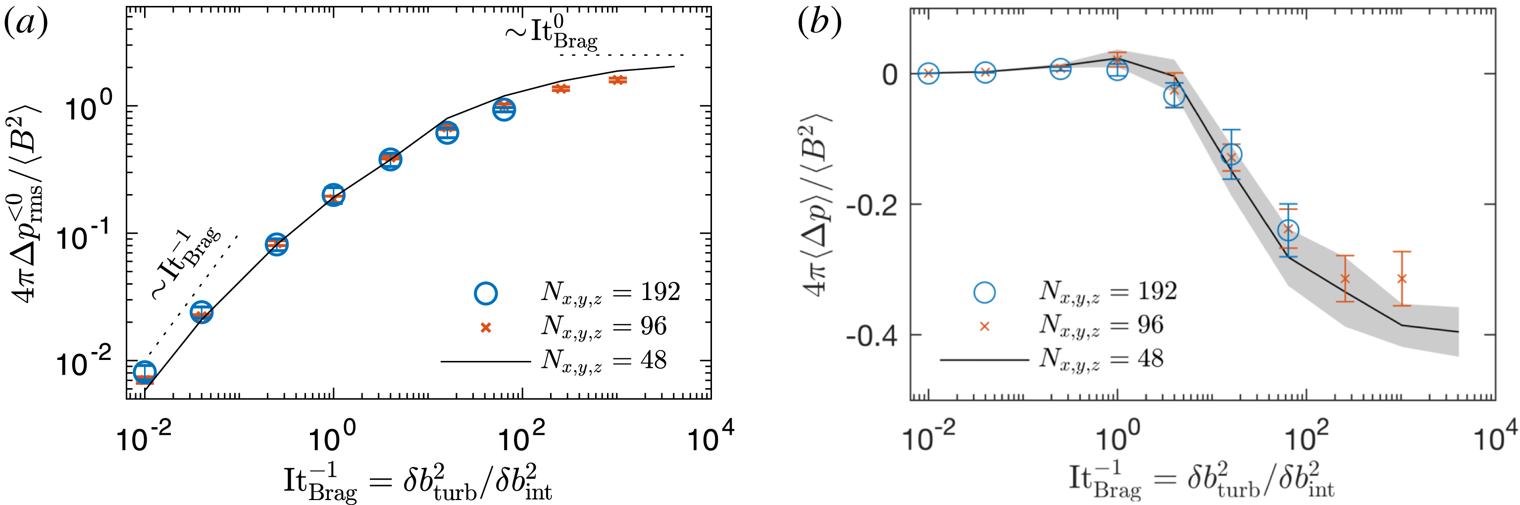
. Figures 5 and 6 provide numerical evidence that this is the case. In particular, we see that key statistical properties of the turbulence appear to reach an asymptotic regime as
 $\text{It}_{\text{Brag}}$
decreases. Figure 5(a) shows that the width of the
 $\unicode[STIX]{x0394}p$
distribution changes from scaling as
 $(\unicode[STIX]{x0394}p)_{\text{rms}}\sim \text{It}_{\text{Brag}}^{-1}$
for
 $\text{It}_{\text{Brag}}\gg 1$
, to
 $(\unicode[STIX]{x0394}p)_{\text{rms}}\sim \text{const}.$
when
 $\text{It}_{\text{Brag}}\ll 1$
. As discussed below (see (2.5)), this scaling demonstrates that pressure-anisotropy forces decrease
 $\hat{\boldsymbol{b}}\hat{\boldsymbol{b}}\boldsymbol{ : }\unicode[STIX]{x1D735}\boldsymbol{u}$
so that the pressure-anisotropy stress is always comparable to
 $\boldsymbol{B}\boldsymbol{\cdot }\unicode[STIX]{x1D735}\boldsymbol{B}$
, even as
 $\unicode[STIX]{x1D707}_{\text{Brag}}$
increases. The turbulence thus becomes more and more magneto-immutable. We also show, in figure 5(b), the mean pressure anisotropy
 $4\unicode[STIX]{x03C0}\langle \unicode[STIX]{x0394}p\rangle /\langle B^{2}\rangle$
as a function of
 $\text{It}_{\text{Brag}}$
. This appears to approach
 $\langle \unicode[STIX]{x0394}p\rangle \approx -0.4\langle B^{2}\rangle /4\unicode[STIX]{x03C0}$
at
 $\text{It}_{\text{Brag}}\ll 1$
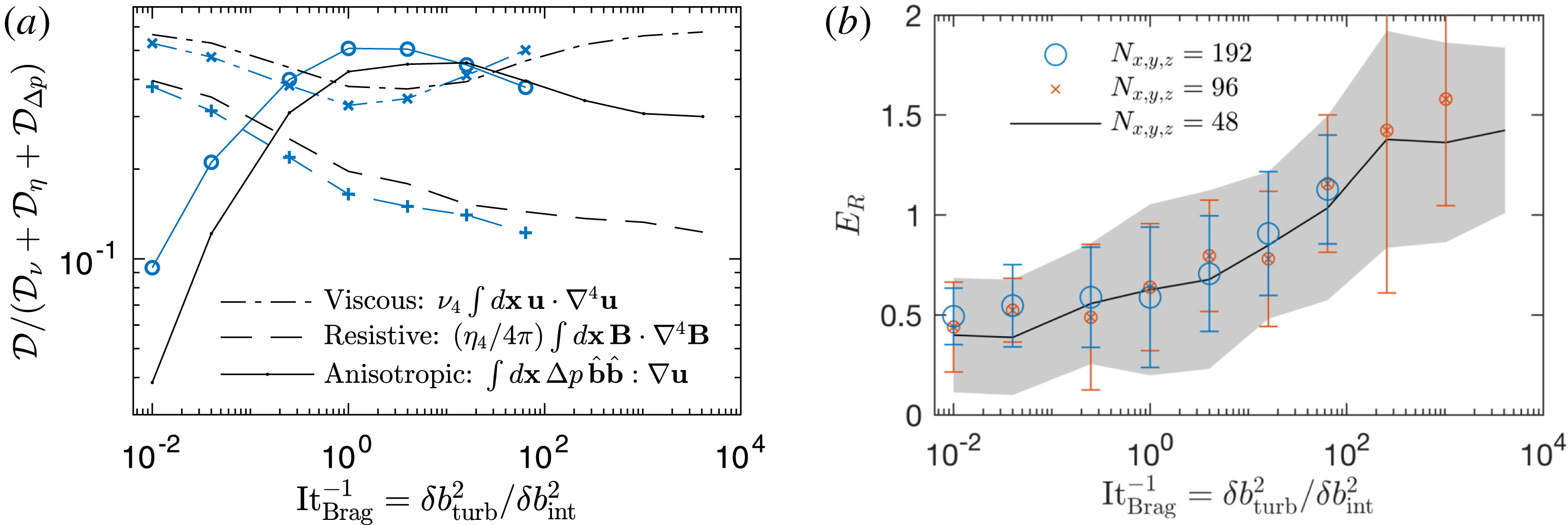
. Finally, in figure 6(a), we compare the turbulent dissipation due to Braginskii viscosity,
 ${\mathcal{D}}_{\unicode[STIX]{x0394}p}\equiv \int \text{d}\boldsymbol{x}\unicode[STIX]{x0394}p\hat{\boldsymbol{b}}\hat{\boldsymbol{b}}\boldsymbol{ : }\unicode[STIX]{x1D735}\boldsymbol{u}$
, with that due to hyper-viscosity and hyper-resistivity. Because
 $\hat{\boldsymbol{b}}\hat{\boldsymbol{b}}\boldsymbol{ : }\unicode[STIX]{x1D735}\boldsymbol{u}$
is unaffected by magneto-immutability in mirror-limiter regions, while
 $(\unicode[STIX]{x0394}p)_{\text{rms}}$
remains approximately constant with
 $\text{It}_{\text{Brag}}$
, the fraction of energy dissipated by Braginskii viscosity remains approximately constant for
 $\text{It}_{\text{Brag}}\lesssim 1$
.
Scaling of
 $\unicode[STIX]{x0394}p$
statistics with
 $\text{It}_{\text{Brag}}$
in the
 $\unicode[STIX]{x1D6FF}b_{\text{turb}}\equiv \unicode[STIX]{x1D6FF}B_{\bot }/B_{0}\approx 1$
(
 $L_{x}=1$
) simulations with a mirror, but no firehose, limiter. We compare simulation sets with varying resolution in order to explore the
 $\text{It}_{\text{Brag}}\ll 1$
regime of magneto-immutable turbulence. (a) Width of the
 $\unicode[STIX]{x0394}p$
distribution, calculated for
 $\unicode[STIX]{x0394}p<0$
, where the pressure anisotropy is not artificially limited (
 $\unicode[STIX]{x0394}p_{\text{rms}}^{{<}0}\equiv \langle \unicode[STIX]{x0394}p^{2}|_{\unicode[STIX]{x0394}p<0}\rangle ^{1/2}$
; see figure 4, thick blue line). The convergence of
 $4\unicode[STIX]{x03C0}\unicode[STIX]{x0394}p_{\text{rms}}^{{<}0}/\langle B^{2}\rangle$
to approximately 2 at
 $\text{It}_{\text{Brag}}\ll 1$
shows that the flow becomes increasingly magneto-immutable with decreasing
 $\text{It}_{\text{Brag}}$
. (b) Mean pressure anisotropy in each simulation, which also appears to converge to an asymptotic value
 $4\unicode[STIX]{x03C0}\langle \unicode[STIX]{x0394}p\rangle \approx -0.4\langle B^{2}\rangle$
at
 $\text{It}_{\text{Brag}}\ll 1$
. Error bars in each panel show the temporal dispersion of the plotted quantities.

Scaling properties of turbulence statistics in the trans-Alfvénic (
 $\unicode[STIX]{x1D6FF}b_{\text{turb}}\equiv \unicode[STIX]{x1D6FF}B_{\bot }/B_{0}\approx 1$
) mirror-limited simulations, using the same conventions as figure 5. (a) Dissipation
 ${\mathcal{D}}$
(energy lost per
 $\unicode[STIX]{x1D70F}_{A}$
) due to
 $\unicode[STIX]{x0394}p$
(
 ${\mathcal{D}}_{\unicode[STIX]{x0394}p}\equiv \int \text{d}\boldsymbol{x}\unicode[STIX]{x0394}p\hat{\boldsymbol{b}}\hat{\boldsymbol{b}}\boldsymbol{ : }\unicode[STIX]{x1D735}\boldsymbol{u}$
; solid lines), and due to hyper-viscosity (
 ${\mathcal{D}}_{\unicode[STIX]{x1D708}}\equiv \unicode[STIX]{x1D708}_{4}\int \text{d}\boldsymbol{x}\boldsymbol{u}\boldsymbol{\cdot }\unicode[STIX]{x1D6FB}^{4}\boldsymbol{u}$
; dashed lines) and hyper-resistivity (
 ${\mathcal{D}}_{\unicode[STIX]{x1D702}}\equiv (\unicode[STIX]{x1D702}_{4}/4\unicode[STIX]{x03C0})\int \text{d}\boldsymbol{x}\boldsymbol{B}\boldsymbol{\cdot }\unicode[STIX]{x1D6FB}^{4}\boldsymbol{B}$
; dot-dashed lines), with values normalized to the total dissipation rate
 ${\mathcal{D}}_{\unicode[STIX]{x1D708}}+{\mathcal{D}}_{\unicode[STIX]{x1D702}}+{\mathcal{D}}_{\unicode[STIX]{x0394}p}$
. Blue lines with symbols show
 $N_{x,y,z}=192$
simulations, black lines show
 $N_{x,y,z}=48$
simulations. The anisotropic diffusion remains approximately constant for
 $\text{It}_{\text{Brag}}\lesssim 1$
, despite the increasing
 $\unicode[STIX]{x1D707}_{\text{Brag}}$
. (b) Turbulent residual energy
 $E_{R}$
. We see tentative evidence for the approach to an asymptotic value
 $E_{R}\approx 1.5$
as
 $\text{It}_{\text{Brag}}\rightarrow 0$
, again suggesting that the turbulence has a well-defined magneto-immutable state for
 $\text{It}_{\text{Brag}}\ll 1$
.

Finally, the existence of this asymptotic regime in the statistics of
 $\unicode[STIX]{x0394}p$
as
 $\text{It}_{\text{Brag}}\rightarrow 0$
suggests that the system can reach a well-defined magneto-immutable turbulent state, where turbulence properties – e.g. velocity and field statistics – do not depend on
 $\text{It}_{\text{Brag}}$
. This is possible because the typical size of the Braginskii viscous stress in the momentum equation,
 $\unicode[STIX]{x1D735}\boldsymbol{\cdot }(\hat{\boldsymbol{b}}\hat{\boldsymbol{b}}\unicode[STIX]{x0394}p)$
, can become independent of
 $\unicode[STIX]{x1D707}_{\text{Brag}}$
. Similar ideas are widely applied to compressible hydrodynamic turbulence, where the properties of the velocity field become effectively independent of Mach number
 ${\mathcal{M}}$
for
 ${\mathcal{M}}\ll 1$
. We give tentative evidence that our simulations approach this asymptotic magneto-immutable turbulence in figure 6(b), which shows that the turbulent residual energy
 $E_{R}$
appears to approach a constant value for
 $\text{It}_{\text{Brag}}^{-1}\gtrsim 300$
. However, we caution that the details of this asymptotic state – e.g. the value of
 $E_{R}$
as
 $\text{It}_{\text{Brag}}\rightarrow 0$
– depend on the limiters used and the Braginskii MHD model. Furthermore, reaching this asymptotic state is computationally very challenging due to the enormous
 $\unicode[STIX]{x1D707}_{\text{Brag}}$
, and our lowest
 $\text{It}_{\text{Brag}}$
simulations may be suspect due to their very low resolutions (
 $N_{x,y,z}=48$
). The study of detailed flow and field structures and/or statistics (e.g. scale-dependent anisotropy) at such a low resolution is of questionable utility, so it remains an open question how the properties of the turbulence at asymptotically low
 $\text{It}_{\text{Brag}}$
differ from those at moderate
 $\text{It}_{\text{Brag}}$
or in MHD (although it is worth noting that energy spectra at
 $\text{It}_{\text{Brag}}\approx 1/64^{2}$
are similar to those at lower
 $\text{It}_{\text{Brag}}$
; see the inset of figure 3
a). There is also clearly much further work needed in order to understand
 $\text{It}_{\text{Brag}}\rightarrow 0$
turbulence in less collisional plasmas where
 $\unicode[STIX]{x1D708}_{c}\lesssim \unicode[STIX]{x1D6FD}^{1/2}\unicode[STIX]{x1D714}_{A}$
and the Braginskii MHD model does not apply.
4 Conclusions
We propose that weakly collisional and collisionless plasma turbulence is often ‘magneto-immutable’ – that is, it self-organizes to resist changes to
 $|\boldsymbol{B}|$
by minimizing
 $|\hat{\boldsymbol{b}}\hat{\boldsymbol{b}}\boldsymbol{ : }\unicode[STIX]{x1D735}\boldsymbol{u}|$
. This occurs due to the pressure-anisotropy stress
 $\unicode[STIX]{x1D735}\boldsymbol{\cdot }(\hat{\boldsymbol{b}}\hat{\boldsymbol{b}}\unicode[STIX]{x0394}p)$
, somewhat analogously to the way in which bulk pressure forces (and bulk viscosity) render fluids incompressible. In Alfvénic turbulence, our focus here, the effect is relevant for all scales above the plasma’s kinetic microscales, and for fluctuation amplitudes around and above the ‘interruption limit’ (1.2) (Squire et al.
Reference Squire, Quataert and Schekochihin2016). By analogy with the Reynolds number, we define the turbulent ‘interruption number’
 $\text{It}_{\text{Brag}}$
, which is the ratio of the ‘pressure-anisotropy time scale’ (the time scale required to generate
 $|\unicode[STIX]{x0394}p|\sim B^{2}$
) to the inertial time scale of the turbulence. Turbulence becomes magneto-immutable for
 $\text{It}_{\text{Brag}}\lesssim 1$
, which, for trans-Alfvénic fluctuations (
 $\unicode[STIX]{x1D6FF}B_{\bot }\sim B$
), occurs when
 $\unicode[STIX]{x1D6FD}\gtrsim \unicode[STIX]{x1D708}_{c}/\unicode[STIX]{x1D714}_{A}$
in a weakly collisional plasma, or when
 $\unicode[STIX]{x1D6FD}\gtrsim 1$
in a collisionless plasma. While kinetic microinstabilities frustrate the plasma’s attempts to become magneto-immutable by breaking the adiabatic link between
 $\hat{\boldsymbol{b}}\hat{\boldsymbol{b}}\boldsymbol{ : }\unicode[STIX]{x1D735}\boldsymbol{u}$
and
 $\unicode[STIX]{x0394}p$
, they cannot eliminate the effect, even if they instantaneously constrain
 $\unicode[STIX]{x0394}p$
to lie within the region of stability (
 $|\unicode[STIX]{x0394}p|/p_{0}\lesssim \unicode[STIX]{x1D6FD}^{-1}$
).
We confirm these ideas using driven magnetized-turbulence simulations in the weakly collisional Braginskii MHD model, which contains the key physics without truly kinetic complications. The resulting magneto-immutable turbulence strongly resembles Alfvénic MHD turbulence, displaying similar energy spectra and scale-dependent anisotropy, although it exhibits a somewhat larger residual energy. This similarity is particularly surprising given that isolated linearly polarized shear Alfvén waves – generally considered to be the building blocks of MHD turbulence – would be interrupted and unable to propagate for fluctuation amplitudes similar to those seen in the turbulence. To get around this, it appears that the turbulent flow self-organizes into a nonlinear analogue of circular polarization, with tightly curled flow structures that avoid changing
 $B$
(see figure 2). Examination of the probability density function of
 $\hat{\boldsymbol{b}}\hat{\boldsymbol{b}}\boldsymbol{ : }\unicode[STIX]{x1D735}\boldsymbol{u}$
(related to
 $\unicode[STIX]{x0394}p$
through
 $\unicode[STIX]{x0394}p=\unicode[STIX]{x1D707}_{\text{Brag}}\hat{\boldsymbol{b}}\hat{\boldsymbol{b}}\boldsymbol{ : }\unicode[STIX]{x1D735}\boldsymbol{u}$
in Braginskii MHD) shows that the turbulence strongly reduces the probability of fluctuations that generate high
 $\hat{\boldsymbol{b}}\hat{\boldsymbol{b}}\boldsymbol{ : }\unicode[STIX]{x1D735}\boldsymbol{u}$
compared to MHD, without significantly reducing amplitude of the
 $\boldsymbol{u}$
and
 $\boldsymbol{B}$
fluctuations themselves. This effect is analogous to low-Mach-number hydrodynamic fluctuations self-organizing to reduce the probability of high
 $\unicode[STIX]{x1D735}\boldsymbol{\cdot }\boldsymbol{u}$
. In the limit of very high
 $\unicode[STIX]{x1D6FD}$
(
 $\text{It}_{\text{Brag}}\rightarrow 0$
or
 $\unicode[STIX]{x1D707}_{\text{Brag}}\rightarrow \infty$
), we see tentative evidence that the turbulence approaches a well-defined magneto-immutable state, where the statistics of
 $\boldsymbol{u}$
and
 $\boldsymbol{B}$
no longer depend on the Braginskii viscosity (i.e.
 $\text{It}_{\text{Brag}}$
). Again, this is analogous to how the statistics of
 $\boldsymbol{u}$
become independent of Mach number as subsonic turbulence becomes incompressible.
A promising application of the ideas discussed throughout this work would be to MHD-scale turbulence in the collisionless solar wind, although the characteristics of magneto-immutability in the collisionless regime are admittedly still to be investigated at the present time. While many studies have found that solar-wind turbulence is well described by MHD models (Matthaeus et al.
Reference Matthaeus, Wan, Servidio, Greco, Osman, Oughton and Dmitruk2015; Chen Reference Chen2016), we predict a key difference: that the distribution of
 $\hat{\boldsymbol{b}}\hat{\boldsymbol{b}}\boldsymbol{ : }\unicode[STIX]{x1D735}\boldsymbol{u}$
should be much narrower than what would be driven by unconstrained (non-magneto-immutable) fluctuations of similar amplitude (see figure 4). Intriguing evidence for this can be found in observations that show
 $\boldsymbol{B}$
fluctuations preferentially trace out the surface of a sphere, keeping
 $|\boldsymbol{B}|$
approximately constant (see, e.g. figure 4 of Bruno et al.
Reference Bruno, Carbone, Veltri, Pietropaolo and Bavassano2001, as well as Lichtenstein & Sonett Reference Lichtenstein and Sonett1980; Tu & Marsch Reference Tu and Marsch1993; Tsurutani et al.
Reference Tsurutani, Ho, Smith, Neugebauer, Goldstein, Mok, Arballo, Balogh, Southwood and Feldman1994; Riley et al.
Reference Riley, Sonett, Tsurutani, Balogh, Forsyth and Hoogeveen1996). A magneto-immutability-based explanation for this behaviour differs somewhat from the recent work of Tenerani & Velli (Reference Tenerani and Velli2018), who argue that constant-
 $B$
fluctuations arise directly from the parallel firehose instability. It is, however, consistent with the work of Vasquez & Hollweg (Reference Vasquez and Hollweg1998), who saw constant-
 $B$
states emerging in (hybrid) kinetic simulations. Further work on collisionless plasmas, as well as some understanding of magneto-immutability in an imbalanced cascade, is necessary before making detailed comparisons to solar-wind data.
On the theoretical side, a thought-provoking (if esoteric) question, is whether it is possible to formulate directly and solve the equations for a truly magneto-immutable fluid, just as the incompressible fluid equations constitute a valuable model for subsonic fluid dynamics. There remain many open questions related to the structure of magneto-immutable turbulence – for instance, how it is able to remain so similar to Alfvénic MHD turbulence – which will require higher-resolution simulations to address in detail. It is also important to move beyond the incompressible, high-collisionality Braginskii MHD model used here, exploring the influence of heat fluxes on pressure-anisotropy stresses (Mikhailovskii & Tsypin Reference Mikhailovskii and Tsypin1971), how magneto-immutability effects interact with density fluctuations (i.e. compressibility), the physics of magneto-immutability in the collisionless regime and the role of realistic microinstability evolution (e.g. Kunz et al. Reference Kunz, Schekochihin and Stone2014; Melville et al. Reference Melville, Schekochihin and Kunz2016). These questions can be tackled in future work using Landau-fluid models (Snyder et al. Reference Snyder, Hammett and Dorland1997; Santos-Lima et al. Reference Santos-Lima, de Gouveia Dal Pino, Kowal, Falceta-Gonçalves, Lazarian and Nakwacki2014; Sulem & Passot Reference Sulem and Passot2015) and/or MHD-scale kinetic simulations.
Acknowledgements
We thank S. Cowley, P. Kempski, R. Meyrand and M. Strumik for enlightening discussions. Support for J.S. was provided by the Marsden Fund grant UOO1727 managed through the Royal Society Te Apārangi, and by the Gordon and Betty Moore Foundation through grant GBMF5076 to L. Bildsten, E. Quataert and E. Sterl Phinney. The work of A.A.S. was supported in part by grants from UK STFC (ST/N000919/1) and EPSRC (EP/M022331/1). E.Q. was supported by Simons Investigator awards from the Simons Foundation and NSF grants AST 13-33612 and AST 17-15054. M.W.K. was supported in part by NASA grant NNX17AK63G, US DOE Contract DE-AC02-09-CH11466 and an Alfred P. Sloan Research Fellowship. This work used the Extreme Science and Engineering Discovery Environment (XSEDE), which is supported by National Science Foundation grant no. ACI-1548562. Computations were carried out on the Comet system at the San Diego Supercomputing Center, through allocation TG-AST160068. Some of the numerical calculations presented in this work were done on Caltech’s Wheeler cluster.