1 Introduction
The transition regime between continuum and free-molecular flow (
 $0.01<Kn<10$
) poses challenges for evaluating heat flux and drag on high-speed vehicles. The Knudsen number is defined as the ratio of the mean free path (
 $\unicode[STIX]{x1D706}$
) to the length scale of interest (
 $l_{c}$
),
 $Kn\equiv \unicode[STIX]{x1D706}/l_{c}$
, where relevant length scales may include geometry scales, or local gradient scales within the flow. Heating and drag correlations are typically based in continuum theory with expressions derived using approximations of the Navier–Stokes equations, which are not valid for transitional flow. Examples include the heat flux correlation from Fay & Riddell (Reference Fay and Riddell1958) as well as the correlation from Sutton & Graves (Reference Sutton and Graves1971).
For hypersonic flows, gas chemistry (such as dissociation) and radiation from the shock layer to the vehicle surface can be important. Recently, Brandis & Johnston (Reference Brandis and Johnston2014) used computational fluid dynamics (CFD) simulations to construct a new heat flux correlation for stagnation point heating on spherical geometries. An exhaustive set of CFD simulations were performed (Brandis & Johnston Reference Brandis and Johnston2014) using NASA’s CFD code LAURA (Mazaheri & Kleb Reference Mazaheri, Gnoffo, Johnston and Kleb2010) to compute flow fields and convective heating, in addition to NASA’s NEQAIR (Whiting et al.
Reference Whiting, Park, Liu, Arnold and Paterson1996) and HARA (Johnston, Hollis & Sutton Reference Johnston, Hollis and Sutton2008a
,Reference Johnston, Hollis and Sutton
b
) codes to compute radiative heating. The simulation data were used to develop expressions for convective and radiative stagnation point heat flux in function of free-stream velocity (
 $V_{\infty }$
), free-stream density (
 $\unicode[STIX]{x1D70C}_{\infty }$
) and the nose radius (
 $R_{N}$
) of the spherical geometry. Considering their simplicity, the expressions captured the high-fidelity CFD and radiation predictions with sufficient accuracy for many types of engineering analyses. However, the maximum Knudsen number considered, based on free-stream conditions and nose radius, was approximately
 $Kn_{\infty }=0.0136$
. Specifically, this corresponded to a free-stream diatomic nitrogen gas, with
 $\unicode[STIX]{x1D70C}_{\infty }=1.0\times 10^{-5}~\text{kg}~\text{m}^{-3}$
,
 $T_{\infty }=180$
K and
 $R_{N}=0.2$
m. Indeed, it is well established that the transport terms in the Navier–Stokes equations begin to become inaccurate for
 $Kn>0.01$
(Boyd, Chen & Candler Reference Boyd, Chen and Candler1995).
In this article, we present an exhaustive set of direct simulation Monte Carlo (DSMC) calculations, accurate for higher Knudsen number flows. We then construct a new correlation for stagnation point heat flux to spherical geometries using the DSMC results. The functional form of the heat flux correlation was derived theoretically from the Burnett and super-Burnett equations in a recent article by the authors (Singh & Schwartzentruber Reference Singh and Schwartzentruber2016). This physics-based correlation acts as a correction to any continuum correlation developed for low Knudsen number flows (such as the correlation from Brandis & Johnston Reference Brandis and Johnston2014). A correlation for the local heat flux around the sphere is also constructed based on the DSMC results. In addition, using the DSMC results combined with other data from the literature (Tsien Reference Tsien1946; Cheng Reference Cheng1961; Bird Reference Bird1970; Macrossan Reference Macrossan2007), we construct a correlation for the drag coefficient for flow over a sphere at any Knudsen number. In the limit of free-molecular flow, the new heat flux and drag correlations also reproduce the exact analytical expressions from free-molecular flow theory.
2 Correlation expressions
2.1 Stagnation point heat flux
In a recent study by the authors (Singh & Schwartzentruber Reference Singh and Schwartzentruber2016), the Burnett and super-Burnett equations were used to derive an expression for the stagnation point heat flux for high-speed flow over a sphere in the transition regime. The resulting expression acts as a correction to the Fourier heat flux term (the Navier–Stokes heat flux prediction,
 $q_{NS}$
),
 $$\begin{eqnarray}\displaystyle \frac{q}{q_{NS}}=1+h_{r^{1}}+h_{r^{2}}+\cdots \,, & & \displaystyle\end{eqnarray}$$
with
 $$\begin{eqnarray}\displaystyle h_{r^{n}}\approx \left[\unicode[STIX]{x1D6FD}_{n}\frac{\sqrt{\unicode[STIX]{x1D6FE}}(\unicode[STIX]{x1D6FE}-1)^{\unicode[STIX]{x1D714}+3/2}}{2^{2\unicode[STIX]{x1D714}}(\unicode[STIX]{x1D6FE}+1)}\left(1+\frac{T_{w}}{T_{s}}\right)^{\unicode[STIX]{x1D714}}W_{r}\right]^{n}\quad n=1,2,3\ldots . & & \displaystyle\end{eqnarray}$$
Here
 $\unicode[STIX]{x1D6FE}$
is the ratio of specific heats,
 $T_{w}$
is the wall temperature,
 $T_{s}$
is an estimate of the post-shock temperature from normal shock wave theory (
 $T_{s}/T_{\infty }\approx (\unicode[STIX]{x1D6FE}-1)M_{\infty }^{2}/2$
),
 $\unicode[STIX]{x1D714}$
is the viscosity temperature exponent (
 $\unicode[STIX]{x1D707}\propto T^{\unicode[STIX]{x1D714}}$
) and
 $W_{r}$
is the ‘rarefaction parameter’ defined as,
 $$\begin{eqnarray}\displaystyle W_{r}\equiv \frac{M_{\infty }^{2\unicode[STIX]{x1D714}}}{Re_{\infty }}, & & \displaystyle\end{eqnarray}$$
which is the most dominant term, where
 $Re=\unicode[STIX]{x1D70C}V_{\infty }R_{N}/\unicode[STIX]{x1D707}$
,
 $R_{N}$
is the radius and
 $V_{\infty }$
is the free-stream velocity. Finally,
 $\unicode[STIX]{x1D6FD}_{n}$
is a constant that lumps together a number of terms including collision integral constants that appear in the Bhatnagar–Gross–Krook (BGK) Burnett equations. As detailed in Singh & Schwartzentruber (Reference Singh and Schwartzentruber2016), there is some degree of uncertainty in these terms, however they are of order unity and therefore do not contribute significantly to the heat flux expression.
The complete derivation, including all assumptions, is contained in Singh & Schwartzentruber (Reference Singh and Schwartzentruber2016). To summarize, the derivation begins with the full nonlinear BGK Burnett equations (Agarwal, Yun & Balakrishnan Reference Agarwal, Yun and Balakrishnan2001). Although there are a number of variants of the Burnett, super-Burnett and other higher-order equations (Singh & Agrawal Reference Singh and Agrawal2016) in the literature, the BGK Burnett equations (Agarwal et al.
Reference Agarwal, Yun and Balakrishnan2001) were chosen since they have been used extensively by previous researchers, they do not suffer from numerical instabilities and they are the only set of equations that include two-dimensional super-Burnett terms, which are required for stagnation point analysis. Many terms are eliminated by symmetry considerations for stagnation line flow, however, the main simplifying assumptions include the use of normal shock wave jump conditions, hypersonic laminar boundary layer theory (Matting Reference Matting1964) and defining a temperature gradient length scale using the shock wave stand-off distance expression from Wen & Hornung (Reference Wen and Hornung1995). By applying the same analysis and assumptions, both the Burnett (
 $n=1$
) and super-Burnett (
 $n=2$
) heat flux terms reduce to the expression in (2.2). There is a dependence on gas properties (
 $\unicode[STIX]{x1D6FE}$
and
 $\unicode[STIX]{x1D714}$
), as well as the ratio of post-shock temperature (
 $T_{s}$
) to wall temperature (
 $T_{w}$
). However, the dominant dependence is on powers of the rarefaction parameter,
 $W_{r}$
.
This rarefaction parameter is proportional to the Knudsen number (
 $W_{r}\propto M_{\infty }Kn_{\infty }$
), and is the same parameter that appears in the Chapman–Enskog velocity distribution function, which captures departure from an equilibrium gas state. For
 $W_{r}\ll 1$
, the Fourier (Navier–Stokes) heat flux is recovered, however for
 $W_{r}\geqslant 1$
, higher-order terms must be accounted for and the heat flux deviates from the Fourier result. The same rarefaction parameter was also found by Wang, Bao & Tong (Reference Wang, Bao and Tong2010) who performed similar analysis of the Burnett-order heat flux term. By analysing both Burnett and super-Burnett heat flux terms and finding the general result in (2.2), the contributions from all higher-order terms can be inferred (Singh & Schwartzentruber Reference Singh and Schwartzentruber2016).
It can be shown that the wall temperature has a minor effect on heat flux for the high-speed transitional conditions (see figure 2 of Singh & Schwartzentruber Reference Singh and Schwartzentruber2016). Furthermore, since we are presently interested in air (
 $\unicode[STIX]{x1D6FE}\approx 1.4$
and
 $\unicode[STIX]{x1D714}\approx 0.75$
), we further simplify (2.2) as:
 $$\begin{eqnarray}\displaystyle h_{r^{n}}\approx [\unicode[STIX]{x1D6FC}_{n}W_{r}]^{n}, & & \displaystyle\end{eqnarray}$$
where
 $\unicode[STIX]{x1D6FC}_{n}$
are a set of fitting coefficients to be determined next. Evaluating the heat flux using
 $N$
higher-order terms, we have
 $$\begin{eqnarray}\displaystyle q=q_{NS}\left[1+\mathop{\sum }_{n=1}^{n=N}h_{r^{n}}\right]=q_{NS}\left[1+\mathop{\sum }_{n=1}^{n=N}(\unicode[STIX]{x1D6FC}_{n}W_{r})^{n}\right]. & & \displaystyle\end{eqnarray}$$
One could use either (2.2) or (2.4) and determine the fitting coefficients (
 $\unicode[STIX]{x1D6FD}_{n}$
or
 $\unicode[STIX]{x1D6FC}_{n}$
) up to a desired number of terms (
 $n=1,2,\ldots ,N$
), by comparison with accurate heat flux predictions from DSMC, for example.
Finally, in the limit of an infinite series, if one assumes that the
 $\unicode[STIX]{x1D6FC}_{n}$
coefficients are approximately equal, the resulting expression is simply:
 $$\begin{eqnarray}\displaystyle q=\frac{q_{NS}}{1-\unicode[STIX]{x1D6FC}W_{r}}\quad \text{for }-1<\unicode[STIX]{x1D6FC}W_{r}<+1, & & \displaystyle\end{eqnarray}$$
and the heat flux coefficient can be written as
 $$\begin{eqnarray}\displaystyle h_{ct}=\frac{q_{NS}}{\frac{1}{2}\unicode[STIX]{x1D70C}_{\infty }v_{\infty }^{3}(1-\unicode[STIX]{x1D6FC}W_{r})}. & & \displaystyle\end{eqnarray}$$
In this case, only one free parameter (
 $\unicode[STIX]{x1D6FC}$
) needs to be fit, and as shown later in § 4, this simple expression is able to capture the heat flux predicted by DSMC for high speed (
 $M_{\infty }>10.0$
). Lower-speed flows (
 $M_{\infty }\approx 5.0$
) will require wall temperature effects to be taken into account and this is analysed in § 4.2.
Since the above heat flux expression acts as a correction to the Fourier (Naiver–Stokes) result, it is most accurate for moderate values of
 $W_{r}$
. Indeed, for
 $W_{r}\gg 1$
, the flow becomes free molecular and exact analytical expressions for heat flux are available in the literature (Bird Reference Bird1994). The stagnation point heat flux coefficient for a sphere in free-molecular flow (
 $h_{fm}$
), presented here for completeness, is a function of gas properties and Mach number only (i.e. not a function of
 $Kn$
or
 $W_{r}$
),
 $$\begin{eqnarray}\displaystyle q_{fm} & = & \displaystyle \unicode[STIX]{x1D70C}_{\infty }\left(\sqrt{\frac{2k_{B}T_{\infty }}{m}}\right)^{3}\frac{1}{4\sqrt{\unicode[STIX]{x03C0}}}\left\{\left[S_{0}^{2}+\frac{\unicode[STIX]{x1D6FE}}{\unicode[STIX]{x1D6FE}-1}-\frac{\unicode[STIX]{x1D6FE}+1}{2(\unicode[STIX]{x1D6FE}-1)}\frac{T_{w}}{T_{\infty }}\right][\!\text{exp}(-S_{0}^{2})\right.\nonumber\\ \displaystyle & & \displaystyle \left.+\,\sqrt{\unicode[STIX]{x03C0}}S_{0}[1+\text{erf}(\sqrt{\unicode[STIX]{x03C0}}S_{0})]]-\frac{1}{2}\exp (-S_{0}^{2})\right\},\end{eqnarray}$$
where
 $k_{B}$
is the Boltzmann constant,
 $S_{0}=\sqrt{\unicode[STIX]{x1D6FE}/2}M_{\infty }$
and
 $m$
is the molecular mass of gas. The heat flux coefficient based on free-stream conditions is
 $$\begin{eqnarray}\displaystyle h_{fm}=\frac{q_{fm}}{\frac{1}{2}\unicode[STIX]{x1D70C}_{\infty }v_{\infty }^{3}}, & & \displaystyle\end{eqnarray}$$
where the expression involves evaluating the standard error function (
 $\text{erf}(x)$
).
In order to construct a single heat flux correlation, accurate from continuum to the free-molecular conditions, we force our expression (
 $h_{ct}$
) to smoothly asymptote to free-molecular heat flux (
 $h_{fm}$
) by means of bridging function. The final correlation for the stagnation point heat flux coefficient (
 $h_{0}$
) is
 $$\begin{eqnarray}\displaystyle h_{0}=h_{ct}+(h_{fm}-h_{ct})\max \left[\frac{W_{r}-C_{2}}{W_{r}+C_{3}},0\right]. & & \displaystyle\end{eqnarray}$$
This expression combines (2.3), (2.7)–(2.9) which are functions only of free-stream flow parameters and the radius of the spherical geometry. The three fitting parameters (
 $\unicode[STIX]{x1D6FC}$
,
 $C_{2}$
and
 $C_{3}$
) will be determined in the next section through comparison with extensive DSMC simulation results. For now, we note that the condition
 $W_{r}>C_{2}$
dictates the onset of the bridging function to free-molecular flow.
The final correlation for the coefficient of stagnation point heat flux (2.10) also requires the specification of the Fourier heat flux term (
 $q_{NS}$
in (2.7)). In this article, we use the recent correlation developed by Brandis & Johnston (Reference Brandis and Johnston2014) for
 $M_{\infty }>10$
cases, which was based on a large number of CFD calculations and was shown to be accurate for wide range of continuum flow conditions. For completeness, we present here the final expression (Brandis & Johnston Reference Brandis and Johnston2014),
 $$\begin{eqnarray}\displaystyle & q_{NS}=7.455\times 10^{-9}\unicode[STIX]{x1D70C}_{\infty }^{0.4705}V_{\infty }^{3.089}R_{N}^{-0.52},\quad 3\;\text{km}\;\text{s}^{-1}\leqslant V_{\infty }<9.5\;\text{km}\;\text{s}^{-1} & \displaystyle\end{eqnarray}$$
 $$\begin{eqnarray}\displaystyle & q_{NS}=1.270\times 10^{-6}\unicode[STIX]{x1D70C}_{\infty }^{0.4678}V_{\infty }^{2.524}R_{N}^{-0.52},\quad 9.5\;\text{km}\;\text{s}^{-1}\leqslant V_{\infty }<17\;\text{km}\;\text{s}^{-1}, & \displaystyle\end{eqnarray}$$
where
 $q_{NS}$
has units of W cm
 $^{-2}$
,
 $V_{\infty }$
has units of m s
 $^{-1}$
and
 $R_{N}$
has units of m.
It is important to stress that the continuum heat flux correlation of Brandis & Johnston (Reference Brandis and Johnston2014) is based on CFD simulations that employed boundary conditions with no velocity slip or temperature jump. When such a continuum correlation is extrapolated into the transition regime, the no-slip assumption becomes a first-order effect that results in unphysically high heat flux predictions. Ideally, a consistent Chapman–Enskog approximation should be used to derive boundary conditions for the Navier–Stokes equations, which would include velocity slip and temperature jump. As shown in a number of studies, such as those by Gökçen, MacCormack & Chapman (Reference Gökçen, MacCormack and Chapman1987), Gökçen & MacCormack (Reference Gökçen and MacCormack1989), Lofthouse, Scalabrin & Boyd (Reference Lofthouse, Scalabrin and Boyd2008) and Holman & Boyd (Reference Holman and Boyd2009), agreement between DSMC and CFD predictions for heat flux, in the early transition regime, improves significantly when a slip model is used in CFD. It is certainly possible that an improved continuum correlation could be formulated, based on CFD simulations that include an appropriate slip model.
2.2 Total integrated heat flux
Many problems of engineering interest require integrated heat flux as opposed to stagnation point heat flux. We find that the stagnation point heat flux for a sphere can be easily, and accurately, extended to predict the local heat flux over the entire sphere surface. The wake generated by high-speed flow over a sphere is a rather complex flow with no general analytical solution. However, the heat flux to a sphere in the wake region (
 $\unicode[STIX]{x1D703}\geqslant 100^{\circ }$
, where
 $\unicode[STIX]{x1D703}$
is
 $0^{\circ }$
at the stagnation point and is measured in the clockwise direction from the sphere centre) is typically small compared to the forebody heat flux. We find that full DSMC simulation results, in both forebody and wake regions, can be fit by a simple expression.
Murzinov (Reference Murzinov1966) fit an expression for the local heat flux coefficient (
 $h_{\unicode[STIX]{x1D703}c}$
) under continuum hypersonic flow conditions, which is a simple function of the stagnation point heat flux coefficient (
 $h_{0}$
from (2.10)) and
 $\unicode[STIX]{x1D703}$
,
 $$\begin{eqnarray}\displaystyle \frac{h_{\unicode[STIX]{x1D703}c}}{h_{0}}=0.55+0.45\cos (2\unicode[STIX]{x1D703}). & & \displaystyle\end{eqnarray}$$
Based on the DSMC simulation results presented in the next section, we find a noticeable difference between this expression and the DSMC predictions. In the free-molecular regime, based on kinetic theory arguments one can obtain variation of surface heat flux coefficient (
 $h_{\unicode[STIX]{x1D703}fm}$
) in terms of
 $\unicode[STIX]{x1D703}$
as
 $h_{\unicode[STIX]{x1D703}fm}/h_{0}=\cos (\unicode[STIX]{x1D703})$
. A modification to Murzinov (Reference Murzinov1966) fit in (2.13), proposed by Wang et al. (Reference Wang, Bao and Tong2010), uses the weighted mean of
 $h_{\unicode[STIX]{x1D703}c}/h_{0}$
and
 $h_{\unicode[STIX]{x1D703}fm}/h_{0}$
. The final expression, developed by Wang et al. (Reference Wang, Bao and Tong2010) is,
 $$\begin{eqnarray}\displaystyle \frac{h_{\unicode[STIX]{x1D703}}}{h_{0}}=\frac{h_{\unicode[STIX]{x1D703}c}/h_{0}+(W_{r}/3)h_{\unicode[STIX]{x1D703}fm}/h_{0}}{1+W_{r}/3}. & & \displaystyle\end{eqnarray}$$
As shown in the next section, this expression accurately fits our DSMC results, and we recommend the use of this expression (using (2.10) for
 $h_{0}$
) to determine the local heat flux to the sphere surface.
2.3 Total integrated drag (drag coefficient)
There have been many studies devoted to determining the drag coefficient for hypersonic flow over a sphere. Various parameters for correlating the drag coefficient have been proposed. These parameters include
 $Kn$
, breakdown parameters (Bird Reference Bird1970), Tsien’s parameter (
 $M_{\infty }/\sqrt{Re_{\infty }}$
) (Tsien Reference Tsien1946) and the inverse Cheng’s parameter (Cheng Reference Cheng1961). Among these, the inverse Cheng’s parameter has been found to be the better correlating parameter (Macrossan Reference Macrossan2007), and has the following form:
 $$\begin{eqnarray}\displaystyle \frac{1}{K_{C}^{2}}\propto C^{\ast }\frac{M_{\infty }^{2}}{2Re_{\infty }}\quad C^{\ast }=\frac{\unicode[STIX]{x1D707}^{\ast }T_{\infty }}{\unicode[STIX]{x1D707}_{\infty }T^{\ast }}, & & \displaystyle\end{eqnarray}$$
where
 $T^{\ast }$
is the mean of stagnation and wall temperature, and
 $\unicode[STIX]{x1D707}^{\ast }$
is viscosity at that temperature. We have utilized the variable hard sphere (VHS) molecular interaction model to calculate viscosity at any given temperature,
 $$\begin{eqnarray}\displaystyle \unicode[STIX]{x1D707}=\frac{15\sqrt{\unicode[STIX]{x03C0}kmT_{ref}}}{2\unicode[STIX]{x03C0}d_{ref}^{2}(5-2\unicode[STIX]{x1D714})(7-2\unicode[STIX]{x1D714})}\left(\frac{T}{T_{ref}}\right)^{\unicode[STIX]{x1D714}}, & & \displaystyle\end{eqnarray}$$
where
 $\unicode[STIX]{x1D714}=0.74$
,
 $d_{ref}=4.17\times 10^{-10}$
m,
 $T_{ref}=273$
. Interestingly, using
 $\unicode[STIX]{x1D707}\propto T^{\unicode[STIX]{x1D714}}$
and the shock wave jump conditions (
 $T_{s}/T_{\infty }\approx (\unicode[STIX]{x1D6FE}-1)M_{\infty }^{2}/2$
), it can be shown that
 $K_{C}^{2}=aW_{r}$
, where
 $a$
is a function of
 $\unicode[STIX]{x1D6FE}$
, temperature ratio
 $T_{w}/T_{s}$
(
 ${\approx}0$
for
 $M_{\infty }\gg 1$
) and
 $\unicode[STIX]{x1D714}$
only.
Based on the DSMC results presented in the next section, we find that the drag predictions collapse very well with the parameter
 $K_{C}^{2}$
, over a wide range of conditions. Therefore, we propose the following analytical fit for the drag coefficient
 $C_{D}=F_{D}/(1/2)A\unicode[STIX]{x1D70C}_{\infty }V_{\infty }^{2}$
with
 $A=\unicode[STIX]{x03C0}R_{N}^{2}$
as cross-sectional area in following manner,
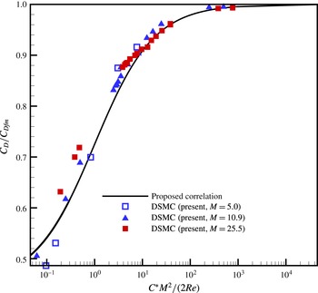
 $$\begin{eqnarray}\displaystyle \frac{C_{D}}{C_{D_{fm}}}=1-\frac{0.55}{C^{\ast }M_{\infty }^{2}/(2Re_{\infty })+1.0}. & & \displaystyle\end{eqnarray}$$
Here,
 $C_{D_{fm}}$
is drag coefficient based on the analytical expression for free-molecular flow derived by Patterson (Reference Patterson1971),
 $$\begin{eqnarray}\displaystyle C_{D_{fm}}=\frac{2S_{0}^{2}+1}{\sqrt{\unicode[STIX]{x03C0}}S_{0}^{3}}\exp (-S_{0}^{2})+\frac{4S_{0}^{4}+4S_{0}^{2}-1}{2S_{0}^{4}}\text{erf}(-S_{0})+\frac{2\sqrt{\unicode[STIX]{x03C0}}}{3S_{0}}\sqrt{\frac{T_{w}}{T_{\infty }}}. & & \displaystyle\end{eqnarray}$$
3 Direct simulation Monte Carlo calculations
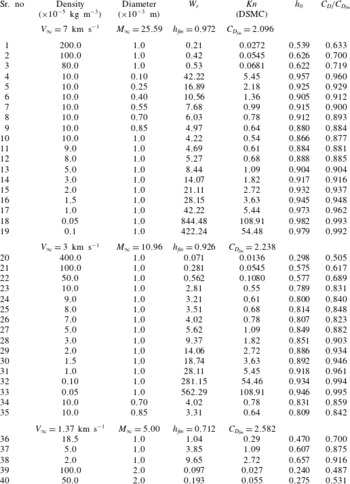
For high-speed flows, the DSMC method (Bird Reference Bird1994) is an accurate and efficient computational method that can provide numerical solutions to the Boltzmann equation. A large number of DSMC calculations are performed for a range of free-stream flow conditions and sphere radii leading to transitional flow conditions (listed in table 1 below). Heat flux and drag values for each simulation (each flow condition) are determined and used to construct heat flux and drag correlations.
Flow conditions, sphere diameter simulated using DSMC.
 $Kn$
is based on sphere diameter, with
 $T_{\infty }=180$
K using VHS model for
 $\unicode[STIX]{x1D706}_{\infty }$
;
 $T_{w}=500$
K.

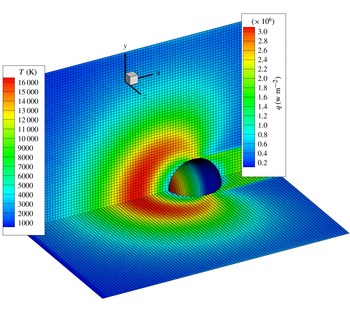
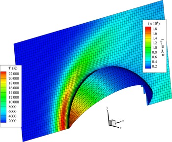
The molecular gas dynamic simulator (MGDS) code (Gao, Zhang & Schwartzentruber Reference Gao, Zhang and Schwartzentruber2011; Nompelis & Schwartzentruber Reference Nompelis and Schwartzentruber2013) is used for this study. The MGDS code is a three-dimensional parallel implementation of the DSMC method developed at the University of Minnesota. Examples of DSMC computed flow fields are shown in figures 1 and 2 for a free-molecular flow condition and a transitional flow condition, respectively. Flow field cells display contours of translational temperature and surface triangles show contours of heat flux. Regardless of the size of flow field cells, the sphere geometry triangulation is the same for all cases, with approximately
 $10\,000$
triangles around the circumference as shown in figures 1 and 2. Cut-cell algorithms (Zhang & Schwartzentruber Reference Zhang and Schwartzentruber2012b
) are used to compute the volumes of cut cells, needed to determine the local collision rate, and to sort surface triangles within cells in order to efficiently detect particle–surface collisions using ray-tracing for particle movement. In DSMC, surface properties are not computed using flow field gradients, rather they are computed by simply recording the total incident momentum (in
 $x$
,
 $y$
and
 $z$
directions) and incident energy for all particles, as well as the momentum and energy of particles leaving the surface, and then taking the time average (in steady state) of the difference to determine the net momentum and energy flux for each surface triangle. Diffuse reflection and full thermal accommodation are assumed for all gas–surface collisions as discussed in further detail below.
DSMC solution for
 $M_{\infty }=25.59$
and
 $Kn=2.72$
.

DSMC solution for
 $M_{\infty }=25.59$
and
 $Kn=0.0272$
.

For high Knudsen number conditions approaching free molecular (figure 1), the DSMC calculations are computationally inexpensive. For these conditions, the computational domain is a box containing one quadrant of the sphere. The centre of the sphere is located on
 $x$
-axis at
 $x\approx 3d$
, where
 $d$
is the sphere diameter. Symmetry boundary conditions are applied along
 $y=0$
and
 $z=0$
planes, and simulation particles are generated upstream of the sphere using equilibrium Maxwell–Boltzmann velocity and internal energy distributions. All other domain boundaries are supersonic outflow boundaries where particles are simply deleted. The domain boundaries are approximately
 $0<x<6d$
,
 $0<y<3d$
and
 $0<z<3d$
. The DSMC result in figure 1 corresponds to
 $Kn=2.72$
. Since such DSMC calculations are computationally inexpensive, it is often appropriate to significantly over-resolve them for visualization purposes and also to avoid the need for local mesh refinement. In this case, the cell size was approximately
 $\unicode[STIX]{x0394}x=0.008\unicode[STIX]{x1D706}_{\infty }$
, the time step was approximately
 $\unicode[STIX]{x0394}t=1\times 10^{-4}\times \unicode[STIX]{x1D70F}_{c-\infty }$
(
 $\unicode[STIX]{x1D70F}_{c-\infty }$
is the free-stream mean collision time) and the total number of simulated particles was approximately 29 million. No flow field grid refinement was necessary.
For lower Knudsen number (transitional flow) conditions (figure 2), the DSMC flow field cells are refined to
 $0.5\unicode[STIX]{x1D706}$
and the time step is set to approximately
 $\unicode[STIX]{x1D70F}_{c}/5$
, where
 $\unicode[STIX]{x1D706}$
and
 $\unicode[STIX]{x1D70F}_{c}$
are the local mean free path and mean collision time, respectively. The simulation is still three-dimensional (3-D), however since flow over a sphere is axisymmetric, a symmetry plane is now introduced by rotating the
 $z=0$
plane by
 $45^{\circ }$
about the
 $x$
-axis in order to reduce computational cost. It is noted that although a 3-D DSMC code along with a Cartesian grid and cut-cell treatment was used for this study, since the problems are axisymmetric, a 2-D/axisymmetric DSMC code with a body-fitted grid could obtain accurate solutions with much less computational time.
The rest of the simulation set-up is the same as for the high Knudsen number cases and, although the number of particles per cell varies widely, there are no fewer than 10 particles per cell. The simulation parameters, time step, number of particles and cell size for each simulation ensured converged results.
In all simulations, the gas consists of diatomic nitrogen with rotational and vibrational energy. For the transitional flows considered, only moderate vibrational energy excitation is observed and chemical reactions are rare. Although oxygen excites and dissociates more rapidly than nitrogen, under transitional conditions and for the purpose of developing simple correlations, the heat flux and drag results from nitrogen simulations are accurately representative of results from air. In the DSMC simulations, chemical reactions are not considered, since for the flows conditions considered, dissociation reactions are rare and have a negligible influence on surface properties. With little dissociation, surface chemical reactions, such as the exothermic recombination of nitrogen and/or oxygen atoms into molecules, also do not contribute significantly to the heat flux and are therefore not considered in the transitional flow simulations. The rotational collision number is constant (
 $Z_{rot}=5$
) and the vibrational collision number (
 $Z_{vib}$
) corresponds to the Millikan–White correlation with Park’s high-temperature correction, where a cell-averaged translational temperature is used to determine
 $Z_{vib}(T)$
(Zhang & Schwartzentruber Reference Zhang and Schwartzentruber2012a
). Post-collision rotational energies are determined using the continuous Borgnakke–Larsen (BL) model, and post-collision vibrational energies are determined used the quantized BL method with the simple harmonic oscillator (SHO) model for energy levels and effective vibrational degrees of freedom (Bergemann & Boyd Reference Bergemann and Boyd1994). The no-time-counter (NTC) method is used along with the VHS collision model. The VHS parameters used for nitrogen are
 $d_{ref}=4.17$
Å,
 $T_{ref}=273$
K and
 $\unicode[STIX]{x1D714}=0.74$
. Finally, diffuse reflection and full thermal accommodation boundary conditions are used for all particle collisions with the sphere surface triangles. For all of the applications discussed in the introduction, this is an excellent assumption since material surface topologies at the atomic level are rugged and impinging particles would undergo multiple collisions before returning to the gas phase. For materials that have smooth surfaces at the atomic and microscale, drag and heat flux values could be significantly below the computed results presented in this article. The model parameters discussed above are well established for non-reacting nitrogen flows and the simulations are expected to provide accurate solutions of the Boltzmann equation including surface properties.
4 Results and discussion
In this section, we present the results of the DSMC calculations for heat flux and drag over a wide range of flow conditions. By comparison with the correlations for heat flux and drag detailed in the previous section, the values of fitting parameters are determined, therefore completing the correlations. Also, by comparison with the DSMC results, the accuracy of the correlations is quantified.
To summarize, the correlation for stagnation point heat flux is given by (2.10), which incorporates (2.3), (2.7)–2.9 as well as the continuum heat flux result of Brandis & Johnston (Reference Brandis and Johnston2014) given in (2.11) and (2.12). Preliminary fitting parameters were previously obtained using limited DSMC results from the literature as
 $\unicode[STIX]{x1D6FC}=-0.476,C_{2}=1.10,C_{3}=1.8$
(Singh & Schwartzentruber Reference Singh and Schwartzentruber2016). The correlation for local heat flux around the sphere surface is the expression from Wang et al. (Reference Wang, Bao and Tong2010) given in (2.14), which incorporates (2.13) and our stagnation point heat flux result from (2.10). The final correlation for the coefficient of drag is given in (2.17), which uses the free-molecular drag result in (2.18) and the inverse Cheng’s parameter in (2.15). All equations are functions of free-stream flow conditions and sphere radius only.
4.1 Stagnation and surface heat flux coefficient
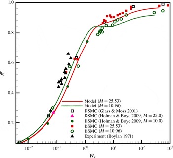
Convective stagnation heat flux coefficient with proposed correlation. Note that data from Glass & Moss (Reference Glass and Moss2001) and Boylan (Reference Boylan1971) correspond to
 $13.3\leqslant M_{\infty }\leqslant 21.42$
and
 $M_{\infty }\approx 21.3$
respectively.

In figure 3, DSMC results for
 $h_{0}$
are plotted for the conditions given in table 1 (
 $M_{\infty }>10$
). Figure 3 also shows DSMC calculations performed by Holman & Boyd (Reference Holman and Boyd2009). Although not shown, it is important to note that the continuum correlation proposed by Brandis & Johnston (Reference Brandis and Johnston2014) begins to significantly over-predict
 $h_{0}$
for
 $W_{r}>0.3$
(see figure 4 in Singh & Schwartzentruber Reference Singh and Schwartzentruber2016). The new correlation (denoted as ‘Model’), employing the preliminary fitting parameters detailed in the preceding paragraph, captures well the variation of
 $h_{0}$
with
 $W_{r}$
in the continuum limit and the variation with
 $M_{\infty }$
in the free-molecular limit. The value of the fitting constant
 $C_{2}$
initiates bridging to the free-molecular limit starting at
 $Kn\approx 7.0$
.
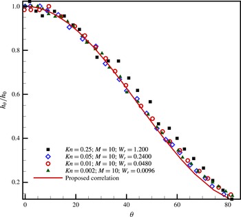
Convective surface heat flux coefficient plotted as a function of
 $\unicode[STIX]{x1D703}$
.

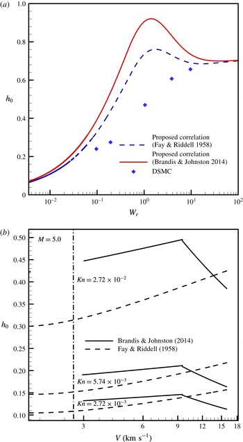
(a) Stagnation point heat flux coefficient (
 $M_{\infty }=5.0$
) using various continuum correlations compared to DSMC results. (b) Fay and Riddell correlation (
 $h_{FR}$
) compared to the Brandis and Johnston correlation.

DSMC results for the normalized heat flux coefficient around the sphere (
 $h_{\unicode[STIX]{x1D703}}$
) are plotted in figure 4 for
 $W_{r}=0.01,0.1,1.0$
and
 $10$
cases. When compared with the correlation given by (2.14), the agreement is remarkably good for
 $\unicode[STIX]{x1D703}<100^{\circ }$
, where a majority of the heat load is experienced.
4.2 Heat flux coefficient for low
 $M_{\infty }$

For lower Mach number conditions (
 $M_{\infty }=5$
), the stagnation point heat flux correlation (2.10) differs significantly from DSMC results as shown in figure 5(a). There are two main reasons for this discrepancy which are remedied in the current section.
First, the Brandis & Johnston (Reference Brandis and Johnston2014) correlation is an empirical correlation fit to CFD calculations of only high Mach number flows, and its direct extension to lower Mach numbers may not be accurate. For example, the Brandis & Johnston (Reference Brandis and Johnston2014) correlation is compared to the Fay & Riddell (Reference Fay and Riddell1958) correlation in figure 5(b). For
 $M_{\infty }<5$
, where gas phase and gas surface chemistry are negligible and the flow exhibits supersonic (rather than hypersonic) behaviour, the Fay & Riddell (Reference Fay and Riddell1958) correlation may be more physically accurate. If our new correlation uses the Fay & Riddell (Reference Fay and Riddell1958) correlation (
 $h_{FR}$
) for
 $q_{NS}$
in (2.7) (assuming a perfect gas), the agreement with DSMC improves, as shown in figure 5(a). For completeness, we present the expression for
 $h_{FR}$
(Fay & Riddell Reference Fay and Riddell1958)
 $$\begin{eqnarray}\displaystyle h_{FR}=\frac{q_{FR}}{(h_{s}-h_{w})}=\unicode[STIX]{x1D705}Pr^{-0.6}(\unicode[STIX]{x1D70C}_{e}\unicode[STIX]{x1D707}_{e})^{0.40}(\unicode[STIX]{x1D70C}_{w}\unicode[STIX]{x1D707}_{w})^{0.1}\sqrt{\left.\frac{\text{d}u}{\text{d}x}\right|_{e}}\times F, & & \displaystyle\end{eqnarray}$$
where
 $\unicode[STIX]{x1D705}=0.57$
for a cylinder and
 $0.763$
for a sphere,
 $Pr({\approx}0.72)$
is the Prandtl number,
 $h$
is enthalpy, the subscript
 $e$
refers to edge of boundary layer and can be approximated by post-shock conditions using jump conditions, the subscript
 $w$
refers to wall and
 $F$
(
 ${\approx}1.0$
for our case) depends on the assumptions about the dissociation chemistry. The edge velocity gradient can be approximated by
 $\sqrt{2RT_{s}}/R_{N}$
(Anderson Reference Anderson2000), where
 $R$
is gas constant.
Second, a significant overshoot in
 $h_{0}$
is evident from the correlations in figure 5(a). This occurs because the onset of the bridging function is controlled by a constant parameter
 $C_{2}$
, when this onset should be a function of Mach number. Wall temperature effects that are more dominant at lower Mach number also contribute to the discrepancy. Interestingly, it turns out that by including the ratio between wall and stagnation temperatures in the correlation, a dependence on Mach number is introduced and the overall agreement with DSMC is improved. Specifically, the analysis carried out by Singh & Schwartzentruber (Reference Singh and Schwartzentruber2016) (summarized in § 2.1 of this article), was for high
 $M_{\infty }$
where simplifications were assumed for the jump equations and the ratio between wall and stagnation temperature was ignored. Without these assumptions, but otherwise using the assumptions outlined in Singh & Schwartzentruber (Reference Singh and Schwartzentruber2016), where
 $\unicode[STIX]{x1D70C}_{s}/\unicode[STIX]{x1D70C}_{\infty }=(\unicode[STIX]{x1D6FE}+1)M_{\infty }^{2}/[2+(\unicode[STIX]{x1D6FE}-1)M_{\infty }^{2}]$
and
 $T_{s}/T_{\infty }=[2\unicode[STIX]{x1D6FE}/(\unicode[STIX]{x1D6FE}+1)^{2}][2+(\unicode[STIX]{x1D6FE}-1)M_{\infty }^{2}]$
, the general expression for
 $h_{r}^{n}$
can be written as (see (3.7) in Singh & Schwartzentruber Reference Singh and Schwartzentruber2016 for comparison):
 $$\begin{eqnarray}\displaystyle h_{r^{n}} & = & \displaystyle \left[\frac{4}{9\unicode[STIX]{x1D6FE}-5}C(\unicode[STIX]{x1D703},\unicode[STIX]{x1D6E4},\ldots )\right]\nonumber\\ \displaystyle & & \displaystyle \times \left[\frac{\unicode[STIX]{x1D6FE}^{\unicode[STIX]{x1D714}+1/2}(\unicode[STIX]{x1D6FE}-1)^{\unicode[STIX]{x1D714}+3/2}}{2^{\unicode[STIX]{x1D714}}(\unicode[STIX]{x1D6FE}+1)^{2\unicode[STIX]{x1D714}+1}}\left(1+\frac{T_{w}}{T_{s}}\right)^{\unicode[STIX]{x1D714}+1}\left(\frac{2}{M_{\infty }^{2}}+\unicode[STIX]{x1D6FE}-1\right)^{\unicode[STIX]{x1D714}}W_{r}\right]^{n}.\end{eqnarray}$$
The equation above can be further modified by using jump conditions for approximating the ratio between wall and stagnation temperatures to yield (see (2.2) for comparison):
 $$\begin{eqnarray}\displaystyle h_{r^{n}}\approx \left[\unicode[STIX]{x1D6FD}_{n}\frac{\unicode[STIX]{x1D6FE}^{\unicode[STIX]{x1D714}+1/2}(\unicode[STIX]{x1D6FE}-1)^{\unicode[STIX]{x1D714}+3/2}}{2^{\unicode[STIX]{x1D714}}(\unicode[STIX]{x1D6FE}+1)^{2\unicode[STIX]{x1D714}+1}}\left(\!1+\frac{T_{w}}{T_{\infty }}\frac{(\unicode[STIX]{x1D6FE}+1)^{2}}{2\unicode[STIX]{x1D6FE}[2+(\unicode[STIX]{x1D6FE}-1)M_{\infty }^{2}]}\right)^{\unicode[STIX]{x1D714}+1}\!\left(\frac{2}{M_{\infty }^{2}}+\unicode[STIX]{x1D6FE}-1\right)^{\unicode[STIX]{x1D714}}\!W_{r}\right]^{n}. & & \displaystyle \nonumber\\ \displaystyle & & \displaystyle\end{eqnarray}$$
Similar to the series evaluation in (2.4)–(2.6), we obtain,
 $$\begin{eqnarray}\displaystyle h_{r^{n}}\approx [\unicode[STIX]{x1D719}_{n}W_{r}^{T}]^{n}\approx [\unicode[STIX]{x1D719}W_{r}^{T}]^{n}, & & \displaystyle\end{eqnarray}$$
however now,
 $$\begin{eqnarray}\displaystyle W_{r}^{T}=\left(1+\frac{T_{w}}{T_{\infty }}\times \frac{(\unicode[STIX]{x1D6FE}+1)^{2}}{2\unicode[STIX]{x1D6FE}[2+(\unicode[STIX]{x1D6FE}-1)M_{\infty }^{2}]}\right)^{\unicode[STIX]{x1D714}+1}\left(\frac{2}{M_{\infty }^{2}}+\unicode[STIX]{x1D6FE}-1\right)^{\unicode[STIX]{x1D714}}W_{r}. & & \displaystyle\end{eqnarray}$$
One final aspect to consider is that, in the limit of
 $M_{\infty }\gg 1.0$
, the coefficient terms in front of
 $W_{r}$
in (4.4) should reduce to the same coefficient (
 $\unicode[STIX]{x1D6FC}=-0.476$
) as determined by the high Mach number analysis in preceding sections. We force this condition in the following manner to evaluate
 $\unicode[STIX]{x1D719}$
:
 $$\begin{eqnarray}\displaystyle \lim _{M_{\infty }\rightarrow \infty }\unicode[STIX]{x1D719}W_{r}^{T}=\unicode[STIX]{x1D719}(\unicode[STIX]{x1D6FE}-1)^{\unicode[STIX]{x1D714}}W_{r}=\unicode[STIX]{x1D6FC}W_{r}\Rightarrow \unicode[STIX]{x1D719}=\unicode[STIX]{x1D6FC}(\unicode[STIX]{x1D6FE}-1)^{-\unicode[STIX]{x1D714}}. & & \displaystyle\end{eqnarray}$$
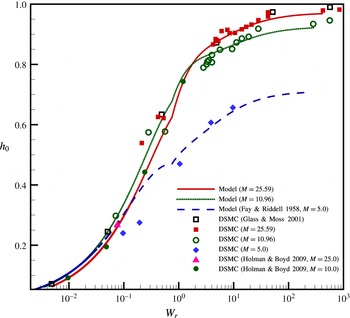
Stagnation heat flux coefficient; final correlation and DSMC results.

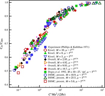
Comparison of DSMC data obtained from MGDS code, experimental data (Phillips & Kuhlthau Reference Phillips and Kuhlthau1971), numerical data available in the literature (Dogra, Wilmoth & Moss Reference Dogra, Wilmoth and Moss1992; Kissel and Overell data reproduced from Macrossan Reference Macrossan2007) for drag coefficient against Cheng’s parameter (Cheng Reference Cheng1961). Experimental data of Phillips & Kuhlthau (Reference Phillips and Kuhlthau1971) correspond to
 $M_{\infty }\approx 8{-}10$
.

4.3 Final correlation for the stagnation point heat flux coefficient
Taking the aforementioned modifications into account, we propose the final correlation:
 $$\begin{eqnarray}\displaystyle h_{0}=h_{ct}+(h_{fm}-h_{ct})\max \left[\frac{W_{r}-C_{2}}{W_{r}+C_{3}},0\right];\quad h_{ct}=\frac{q_{NS}}{\frac{1}{2}\unicode[STIX]{x1D70C}_{\infty }v_{\infty }^{3}(1-\unicode[STIX]{x1D719}W_{r}^{T})}, & & \displaystyle\end{eqnarray}$$
where,
 $$\begin{eqnarray}\displaystyle W_{r}^{T}=\left(1+\frac{T_{w}}{T_{\infty }}\times \frac{(\unicode[STIX]{x1D6FE}+1)^{2}}{2\unicode[STIX]{x1D6FE}[2+(\unicode[STIX]{x1D6FE}-1)M_{\infty }^{2}]}\right)^{\unicode[STIX]{x1D714}+1}\left(\frac{2}{M_{\infty }^{2}}+\unicode[STIX]{x1D6FE}-1\right)^{\unicode[STIX]{x1D714}}W_{r},\quad \unicode[STIX]{x1D719}=\frac{\unicode[STIX]{x1D6FC}}{(\unicode[STIX]{x1D6FE}-1)^{\unicode[STIX]{x1D714}}}. & & \displaystyle \nonumber\\ \displaystyle & & \displaystyle\end{eqnarray}$$
Recall that the preliminary fitting coefficient values, presented at the beginning of § 4, where determined by Singh & Schwartzentruber (Reference Singh and Schwartzentruber2016) based on very limited DSMC results. Based on the new DSMC results of this article (summarized in table 1), we determine better values for these coefficients as
 $$\begin{eqnarray}\displaystyle \unicode[STIX]{x1D6FC}=-0.6\Rightarrow \unicode[STIX]{x1D719}=1.192,\quad C_{2}=0.75,\quad C_{3}=0.75. & & \displaystyle\end{eqnarray}$$
The final correlation (4.7) and (4.8) using these coefficient values is plotted in figure 6 along with our DSMC results and the DSMC results of other researchers. In these results, for
 $M_{\infty }=5$
(4.1) is used for an estimate of
 $q_{NS}$
in (4.7). The agreement is now improved with error less than
 $18\,\%$
for the
 $M_{\infty }=5$
case and less than
 $10\,\%$
for all other conditions. Finally, the trend in
 $h_{0}$
versus
 $Wr$
seen in figure 6 for different Mach numbers can be explained in terms of the free-molecular and continuum limits. For rarefied conditions (high
 $Wr$
) the heat flux coefficient is a function of Mach number only, and therefore
 $h_{0}$
is highest for the Mach
 $25.59$
case and lowest for the Mach
 $5$
case. However, for continuum conditions, for a fixed
 $Wr$
value and a fixed geometry, a higher Mach number condition corresponds to a higher density. In the continuum regime, higher density leads to a reduced
 $h_{0}$
value since the high-temperature gas is diverted around the geometry. Therefore, in the continuum limit (low
 $Wr$
) one might expect increasing Mach number to result in a lower
 $h_{0}$
value. The correlation results in figure 6 are consistent with these expected trends.
4.4 Coefficient of drag
Several correlation parameters for the drag coefficient have been proposed in the literature as summarized by Macrossan (Reference Macrossan2007). Specifically, Macrossan (Reference Macrossan2007) showed that Cheng’s parameter (Cheng Reference Cheng1961) is the best correlation parameter.
In figure 7, our DSMC results (summarized in table 1) are plotted along with a number of results from the literature. All data collapse remarkably well using the inverse Cheng’s parameter, thereby confirming the findings of Macrossan (Reference Macrossan2007). The experimental data of Phillips & Kuhlthau (Reference Phillips and Kuhlthau1971) agree quantitatively with current DSMC results and the results of the literature. The differences between DSMC results can be attributed to different gas species, such as multi-species air for Dogra et al. (Reference Dogra, Wilmoth and Moss1992) and different ratios between free-stream and wall temperatures; approximately unity for Dogra et al. (Reference Dogra, Wilmoth and Moss1992) and Phillips & Kuhlthau (Reference Phillips and Kuhlthau1971), while close to half in our simulations.
Finally, in figure 8, we have plotted our DSMC data and the proposed correlation for the drag coefficient (2.17) that is based on Cheng’s parameter. The correlation matches our DSMC data well for the entire range of Cheng’s parameter. Although the gas species and ratio between free-stream and wall temperatures may alter the precise drag value, we believe that the difference will not be significant and henceforth the proposed correlation should be able to accurately predict drag for all conditions.
Comparison of DSMC data obtained from MGDS code and proposed correlation for drag coefficient against Cheng’s parameter (Cheng Reference Cheng1961).

5 Conclusions
In conclusion, we have presented an exhaustive set of DSMC results for heat flux and drag experienced by a sphere at hypersonic flight conditions in the transitional flow regime. The data were used to construct correlations for the stagnation point heat flux, local heat flux around the sphere and integrated drag, as functions of free-stream flow conditions and sphere radius. The functional form of the stagnation point heat flux and drag correlations, in the transitional regime, are physics based with a dominant dependence on a rarefaction parameter,
 $W_{r}=M_{\infty }^{2\unicode[STIX]{x1D714}}/Re_{\infty }$
, where
 $\unicode[STIX]{x1D714}$
is a parameter set by the viscosity law. The correlations smoothly approach the exact free-molecular expression for high values of the rarefaction parameter
 $W_{r}$
. The stagnation point heat flux correlation is formulated as a correction to a continuum (Fourier model) heat flux correlation. We chose to combine the new heat flux correlation with the continuum correlation recently developed by Brandis & Johnston (Reference Brandis and Johnston2014) for
 $M_{\infty }>10.0$
and developed by Fay & Riddell (Reference Fay and Riddell1958) for
 $M_{\infty }=5.0$
. The free parameters of the correlations were fit by comparison with DSMC results.
The final correlations for stagnation point heat flux (4.7)–(4.9), heat flux around the sphere surface (2.13) and (2.14), and integrated drag coefficient (2.17), which include the relevant free-molecular expressions, were validated with DSMC data to accurately reproduce heat flux and drag results spanning continuum conditions to free molecular. The new DSMC results presented in this article were found to be consistent with previous DSMC results from the literature, consistent with continuum CFD results for small values of
 $W_{r}$
, and consistent with free-molecular results for large values of
 $W_{r}$
. The finalized correlations presented in this article extend continuum correlations to enable analysis at higher altitudes and/or smaller geometry radii, and will be useful for engineering analysis of a number of high-speed flow problems.
Acknowledgements
This research was supported by the Air Force Research Laboratory (AFRL), Kirtland AFB, under grant nos. FA9453-14-1-0291 and FA9453-15-1-0071.