

1 Introduction
1.1 Error-driven ranking algorithms
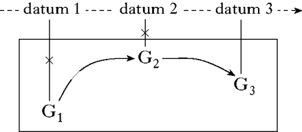
Assume that the learner is provided with the space of all possible grammars G1, G2, etc. Data come in a stream, one piece of data at the time. And the learner maintains a current grammar, which represents its current hypothesis on the target adult grammar. Suppose that at a certain time the current grammar, say G1, fails at accounting for the current piece of data, say datum 1. Prompted by this error, the learner updates the current grammar G1 to a slightly different grammar, G2, which sits nearby in the space of grammars. This process is repeated over and over again, until the learner eventually stops making errors and converges to a final grammar consistent with the stream of input data, so that learning ceases.
Schematic representation of an error-driven learning algorithm.
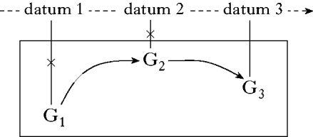
This learning scheme is error-driven, as the learning dynamics is driven by the errors performed on the incoming stream of data. This scheme has been thoroughly investigated in the machine learning literature (under the heading of online learning; for reviews, see Kivinen Reference Kivinen, Mendelson and Smola2003 and Cesa-Bianchi & Lugosi Reference Cesa-Bianchi and Lugosi2006: chs 11, 12). Within the linguistic literature, error-driven learning dates back to at least Wexler & Culicover (Reference Wexler and Culicover1980).
This paper explores error-driven learning within the phonological framework of Optimality Theory (OT; Kager Reference Kager1999, Prince & Smolensky Reference Prince and Smolensky2004). Thus the space of grammars is defined through the set of rankings over a given constraint set. And the slight shift from the current grammar to the updated grammar consists of a slight re-ranking of the constraints. The resulting algorithms are called Error-driven Ranking Algorithms (EDRAs). Two EDRAs that have played an important role in the OT acquisition and computational literature are Tesar & Smolensky's (Reference Tesar and Smolensky1998) Error-driven Constraint Demotion (EDCD) and Boersma's (Reference Boersma1998) Gradual Learning Algorithm (GLA). Building on this literature, §2 offers a detailed introduction to EDRAs.
The intermediate rankings entertained by an EDRA can be interpreted as intermediate learning stages, which model the observed gradual, stepwise child progression towards the target adult language. Furthermore, the model does not keep track of previously seen forms, and thus does not impose unrealistic memory requirements (contrary to batch models, which are allowed to glimpse at the entire set of data at once). For these reasons, most of the OT acquisition literature has endorsed EDRAs as cognitively plausible models of child acquisition; see for instance Bernhardt & Stemberger (Reference Bernhardt and Stemberger1998), Boersma & Levelt (Reference Boersma, Levelt and Clark2000) and Gnanadesikan (Reference Gnanadesikan2004), as well as Tesar (Reference Tesar2004) and Tessier (Reference Tessier2009) for critical discussion and alternative approaches.
Bridging cognitive plausibility with computational soundness, this paper looks at the most basic computational issue in the theory of EDRAs, namely convergence: the EDRA should eventually stop making errors, and thus settle on a final ranking consistent with the incoming stream of data. And convergence should be efficient: the number of errors made by the algorithm before converging should not only be finite, but should furthermore grow slowly with the complexity of the underlying OT typology, measured as the number of constraints. As clearly stated in Keller & Asudeh (Reference Keller and Asudeh2002: 237), ‘convergence is a crucial property of a learning algorithm that should be investigated formally’. This paper develops a complete theory of EDRA convergence, which provides both sufficient and necessary conditions for efficient convergence.
1.2 Summary of the main results
The first EDRA developed in the OT computational literature is Tesar & Smolensky's (Reference Tesar and Smolensky1998) Error-driven Constraint Demotion. Its signature property is that it demotes offending constraints to a lower position, but does not promote virtuous constraints. Lack of constraint promotion allows Tesar & Smolensky (but see Boersma Reference Boersma2009) to prove that EDCD converges and that convergence is efficient, as it is achieved after a worst-case number of errors that grows only quadratically in the number of constraints. Tesar & Smolensky's result sets the standard for the theory of EDRAs. Furthermore, some of the tools used in their analysis turn out to extend beyond demotion-only to EDRAs that perform constraint promotion too. For these reasons, §3 offers a thorough review of Tesar & Smolensky's theory.
Although a virtue from a computational perspective, lack of constraint promotion turns out to be a liability from a modelling perspective. §4 argues for EDRAs that perform constraint promotion on top of demotion, by looking at one of the main modelling applications of EDRAs, namely modelling the early acquisition of phonotactics by the child. In this modelling literature, it is standard to assume that the child posits fully faithful underlying forms. This entails that faithfulness constraints are never responsible for the failure of the current ranking vector. As EDCD only demotes the constraints that are responsible for the current failure (but never promotes those that could have prevented that failure), it thus never re-ranks the faithfulness constraints. This cannot be right. If two languages in the typology require the opposite relative ranking of some faithfulness constraints, EDCD fails on at least one of them (Hayes Reference Hayes2004 and Prince & Tesar Reference Prince and Tesar2004 provide examples of such cases). Furthermore, EDCD is unable to model learning paths where the child's repair strategy for a certain marked structure changes over time (for instance, McLeod et al. Reference McLeod, Doorn and Reed2001 document learning paths where complex onsets are simplified by different strategies over time, such as deletion and coalescence).
Although needed from a modelling perspective, convergent EDRAs that perform both constraint demotion and promotion are not easy to devise. Tesar & Smolensky (Reference Tesar and Smolensky1998) explicitly warn against the danger of constraint promotion. Indeed, there is only one EDRA currently available in the literature that performs both constraint demotion and promotion, namely Boersma's (Reference Boersma1998) GLA. Yet Pater (Reference Pater2008) shows through a simple counterexample that the GLA does not converge in the general case. §5 reviews this literature on constraint promotion. In particular, it contributes the first explicit explanation of the GLA's failure on Pater's counterexample. In conclusion, computationally sound EDRAs that perform both constraint demotion and promotion are needed from the perspective of the OT acquisition literature, but have so far eluded the efforts of the OT computational literature.
This paper resolves this impasse, showing that efficient convergence can be achieved despite constraint promotion, through a proper calibration of the promotion component of the re-ranking rule. I illustrate the idea informally here. Following Boersma (Reference Boersma1997, Reference Boersma1998), I assume throughout this paper that EDRAs entertain a numerical representation of the current ranking, by assigning to each constraint a numerical ranking value, whose relative size reflects the relative ranking of that constraint. Boersma's non-convergent GLA demotes (i.e. decreases the ranking value of) the bad constraints by 1 and promotes (i.e. increases the ranking value of) the good constraints by the same amount, 1. But suppose there are few constraints that need to be demoted, but many constraints that need to be promoted. In this case, the GLA demotes a few times by 1 and promotes many times by 1. Overall, the GLA thus performs more constraint promotion than demotion. Pater's (Reference Pater2008) counterexample shows that this is not a good idea. Indeed, as demotion-only has been shown by Tesar & Smolensky (Reference Tesar and Smolensky1998) to converge efficiently, the promotion component of the re-ranking rule should not overwhelm the demotion component, so as not to disrupt too much its efficient convergence. This requires a proper calibration of the promotion amount, i.e. the amount by which good constraints are promoted. For instance, if there are two constraints that are promoted and one that is demoted, then the promotion amount should intuitively be less than 1/2. In fact, two promotions by less than 1/2 lead to an overall promotion which is less than the overall demotion of 1, so that indeed the overall constraint promotion does not overwhelm constraint demotion. These heuristic considerations suggest that, in the general case, the promotion amount should be smaller than the number of constraints demoted divided by the number of constraints promoted, as stated in (1). A re-ranking rule that satisfies the strict inequality (1) is calibrated.
(1)


§6 shows that a slight extension of Tesar & Smolensky's (Reference Tesar and Smolensky1998) analysis of demotion-only EDRAs ensures convergence for any calibrated promotion/demotion EDRA.
To take a concrete case, the promotion amount can be defined as in (2). For instance, if one constraint is demoted and two promoted, then each of the latter two will be promoted by 1/3, according to (2).
(2)
This re-ranking rule is calibrated, as it obviously satisfies condition (1). §6 shows that an EDRA with the calibrated promotion/demotion re-ranking rule (2) converges after a worst-case number of errors that grows only cubically in the number of constraints. This error-bound compares well with Tesar & Smolensky's (Reference Tesar and Smolensky1998) quadratic error-bound for demotion-only EDRAs.
The ratio between the numbers of demoted and promoted constraints is the calibration threshold. The calibration condition in (1) requires the promotion amount to be strictly smaller than this calibration threshold. What happens if we increase the promotion amount up to the threshold, as in (3)?
(3)
§7 addresses this question, showing that convergence is retained but efficiency is lost: the worst-case number of errors is finite, but grows exponentially in the number of constraints. The analysis of the re-ranking rule (3) will rest on a property of EDRAs that is interesting in its own right: they can never entertain again a ranking (vector) that was found to be inconsistent with a previously seen piece of data. In other words, EDRAs explore the typology in a effective way: although they do not keep track of previously seen data and thus of the errors previously made, they implicitly manage to avoid repeating the same error twice.
Although the results developed in this paper are computational in nature, they have significant cognitive implications, discussed in §§1.3–1.6. The paper is thus also relevant to a non-computational audience. In order to make it accessible, the discussion will be informal.Footnote 1
1.3 Implications for the OT vs. HG framework selection problem
Efficient convergence represents the most basic requirement for computationally sound error-driven learning. It is for this reason that the failure of the GLA on Pater's fatal counterexample has prompted various scholars to explore error-driven learning within frameworks alternative to OT, such as Harmonic Grammar (henceforth HG; Legendre et al. Reference Legendre, Miyata and Smolensky1990a, Reference Legendre, Miyata and Smolenskyb), which is equipped with provably convergent error-driven learning algorithms. For recent applications of error-driven learning within HG, see Jesney & Tessier (Reference Jesney and Tessier2007, Reference Jesney and Tessier2009), Coetzee & Pater (Reference Coetzee and Pater2008) and Boersma & Pater (to appear), as well as Pater (Reference Pater2009) and Magri (to appear b) for general discussion.
The results developed in this paper show that the GLA can be easily ‘fixed’, in the sense that it is possible to develop variants of the GLA for standard OT that provably efficiently converge, through a proper calibration of the promotion amount, as in (1). These results thus show that the computational soundness of error-driven learning should not play any role in the debate concerning the OT vs. HG framework selection problem, as both frameworks come with provably convergent error-driven algorithms.Footnote 2
1.4 Implications for modelling gradience
OT grammars are usually parameterised by combinatorial objects, namely rankings. Yet, as originally noted in Boersma (Reference Boersma1997, Reference Boersma1998), OT typologies can also be easily given a numerical re-parameterisation, as rankings can be represented by assigning to each constraint a numerical ranking value, with the understanding that constraints with large ranking values are ranked above constraints with low ranking values. This technical observation immediately raises the following cognitive question: which one of these two parameterisations is cognitively more adequate? Does the learner actually assume that languages are parameterised by combinatorial objects such as rankings or by continuous objects such as ranking values?
This paper offers a new perspective on this issue. Demotion-only EDRAs (such as Tesar & Smolensky's EDCD in its original formulation) can be implemented in terms of combinatorial rankings, with no need for a numerical re-parameterisation in terms of ranking values. §§5–7 will show in detail that the situation is very different for re-ranking rules that perform constraint promotion on top of constraint demotion. In fact, as anticipated above, the promotion component of the re-ranking rule cannot overwhelm the demotion component. This requires a proper numerical calibration of the promotion amount, as in (1). Hence, constraint promotion is inherently numerical, and thus requires a numerical parameterisation of OT typologies. The choice between demotion-only and demotion/promotion EDRAs thus bears on the issue of the proper parameterisation of OT typologies. §4 will argue that demotion-only is inadequate from a modelling perspective, and that a certain amount of constraint promotion is needed. In conclusion, the computational investigation developed in this paper entails that the proper parameterisation of OT grammars should be in terms of numerical ranking values rather than in terms of combinatorial rankings.
This conclusion in turn has theoretical implications for the choice between OT and alternative frameworks that adopt a weighted, numerical model of constraint interaction, such as HG. In particular, various authors have recently suggested that HG's numerical weights might have an advantage over OT's combinatorial rankings from the perspective of modelling gradience. For instance, Pater (Reference Pater2009: 4) writes:
[I will] illustrate and extend existing arguments for the replacement of OT's ranked constraints with weighted ones: that the resulting theory can be adapted relatively straightforwardly to deal with various types of non-categorical linguistic phenomena.
and observes: ‘HG was in fact originally motivated as an account of gradient syntactic well-formedness’ (2009: 23). Yet if we can collect independent evidence in favour of a numerical representation of OT typologies, then the argument just mentioned in favour of the alleged superiority of HG over OT evaporates.
1.5 Implications for modelling the child acquisition of phonotactics
One of the main applications of EDRAs considered in the literature concerns modelling the child acquisition of phonotactics. §4 offers a quick glimpse at this modelling application. I will argue that this important application requires EDRAs to perform some constraint promotion, so as to motivate the computational developments of §6 and §7. My argument will be twofold. First, I will argue that constraint promotion is needed in order for the sequences of rankings formally predicted by EDRAs to have a chance to match child acquisition paths. Second, I will argue that constraint promotion is also needed in order for the final grammar entertained by EDRAs to have a chance of being restrictive, i.e. correctly ruling out illicit forms, despite the fact that the algorithm is only trained on licit forms.
My discussion of this modelling application in §4 will be cursory, as I will only provide the negative part of the argument, i.e. I will only show that constraint promotion is necessary for restrictiveness and for matching child acquisition paths. I will not provide here the positive part of the argument, namely that constraint promotion is indeed also sufficient for restrictiveness and matching. Nevertheless, this paper represents a first step of a larger research project that I am currently involved in, which tries to establish EDRAs as proper models of the acquisition of phonotactics, both from a computational and a modelling perspective. The next step in this project is Magri (Reference Magri2012b), which presents a detailed discussion of the restrictiveness of EDRAs, expanding substantially on the cursory remarks presented below in §4.4.2.
1.6 Implications for modelling child acquisition paths
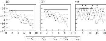
As anticipated above, EDRAs assign to each constraint a numerical ranking value that is updated throughout learning. In Fig. 2, I plot the ranking dynamics for three runs on the same data (the test case considered in Pater Reference Pater2008), with three slightly different choices for the promotion amount. Time is represented on the horizontal axis and ranking values on the vertical axis. Fig. 2b corresponds to the calibrated promotion amount in (2) and Fig. 2a corresponds to a promotion amount only slightly smaller. The two ranking dynamics in (a) and (b) differ only minimally, and the number of updates performed in the two runs is identical. In other words, a small difference in the promotion amounts leads to only small differences in the ranking dynamics, as one might naively expect.
Ranking dynamics predicted by three runs of the EDRA on the same string of input data with three different choices of the promotion amount: (a) p=number of demotions/(number of promotions+2); (b) p=number of demotions/(number of promotions+1); (c) p=number of demotions/(number of promotions).

That is not always the case, though. Figure 2c plots the ranking dynamics on the same data when the promotion amount is equal to the calibration threshold, so that the denominator now coincides with the number of promotions. This promotion amount in (c) differs only very slightly from the one in (b), yet the ranking dynamics in (c) looks completely different, and the number of updates is much larger.
The acquisition of phonology by the child is gradual, in the sense that the target adult phonology is approached through a stepwise progression of intermediate stages. As noted in §1.1, EDRAs have been endorsed in the OT acquisition literature because they offer a way to model gradualness, as acquisition paths can be matched against the sequence of grammars predicted by an EDRA's ranking dynamics. A naive strategy to explore EDRAs' modelling predictions (i.e. how well the predicted ranking dynamics matches attested acquisition paths) would fix the implementation details, such as the choice of the promotion amount, in some heuristic way, based on the assumption that only a few options for the implementation details need to be considered, as the modelling predictions will only vary by small amounts for small variations in the implementation details. But the example in Fig. 2 shows that this assumption is misleading: the behaviour of the algorithm displays breakpoints, at which the modelling predictions of the algorithm change abruptly. Thus, the modelling implications of EDRAs cannot be explored naively, without a preliminary thorough computational understanding of the algorithm and its breakpoints. This paper shows that the calibration threshold represents a crucial breakpoint for the choice of the promotion amount.
2 Error-driven ranking algorithms
§2.1 introduces a basic formulation of EDRAs, following Tesar & Smolensky (Reference Tesar and Smolensky1998). §2.2 restates them in terms of an alternative ERC representation of OT data, after Prince (Reference Prince2002). Finally, §2.3 reformulates them in terms of an alternative numerical parameterisation of OT grammars, after Boersma (Reference Boersma1997, Reference Boersma1998, Reference Boersma2009). §2.4 introduces the issue of EDRAs' convergence.
2.1 Basic description
The basic data unit in OT is a data triplet (4a), consisting of an underlying form /x/ and two surface forms [y] and [z], both drawn from the set Gen(/x/) of candidates for /x/. By convention, the first candidate [y] in the triplet is the intended winner, while the other candidate [z] is an intended loser. As a useful mnemonic, I adopt the convention of striking out the loser. To illustrate, the data triplet (4b) pairs up the underlying form /rad/ with the two candidates [rad] and [rat]. As the former is the intended winner, this triplet says that there is no final devoicing.
(4)
An OT-grammar is parameterised by a ranking, which is a linear order ‘≫’ over the constraint set. Constraint Ch is ≫-ranked above constraint Ck, provided Ch≫Ck. A ranking is (OT-)consistent with an underlying/winner/loser form data triplet (/x/, [y], [z]) provided condition (5) holds. (5) says that the intended loser [z] violates the constraints ‘more severely’ than the intended winner [y], in the sense that, among those constraints that distinguish between the winner [y] and the loser [z], the top ≫-ranked one, Ctop, assigns more violations to the loser than to the winner.
(5)
A ranking is (OT-)consistent with a set of data triplets provided it is consistent with every triplet in the set, and a set of data triplets is (OT-)consistent provided it is consistent with at least one ranking.
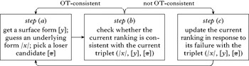
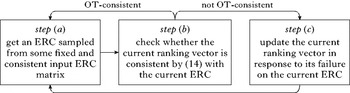
With these preliminaries in place, an EDRA can be described as follows, after Tesar & Smolensky (Reference Tesar and Smolensky1998). The algorithm maintains a current ranking, which represents its current hypothesis on the target grammar. This current ranking is initialised to an initial ranking, and is updated over time by looping through the three steps (a)–(c) in Fig. 3. At step (a), the algorithm assembles an underlying/winner/loser form triplet. At step (b), the algorithm checks the current ranking against the current underlying/winner/loser form data triplet. If the current ranking is consistent with the current data triplet according to (5), nothing happens: the algorithm goes back to step (a) and waits for another piece of data. Otherwise, the algorithm modifies its current ranking at step (c), and then goes back to step (a).
Main loop of an EDRA.

2.2 Restatement in comparative notation
Given an underlying/winner/loser form data triplet (/x/, [y], [z]), the constraints can be sorted into winner-preferring, loser-preferring or even, as in (6), depending on whether they assign more, fewer or the same number of violations to the loser [z] than to the winner [y].
(6)
To illustrate, consider again the data triplet (/rad/, [rad], [rat]) in (4b). The positional faithfulness constraint Fpos=Ident[voice]/Onset for voicing is even, as it does not distinguish between the two candidates [rad] and [rat]. The general faithfulness constraint Fgen=Ident[voice] is winner-preferring, as the intended winner [rad] is fully faithful to the underlying form /rad/, as opposed to the intended loser [rat]. Finally, the markedness constraint M=*[+voice] is loser-preferring, as it is violated by the intended winner [rad], and not by the intended loser [rat].
The definition (5) of OT-consistency does not really care about the actual number of constraint violations. It only cares about whether each constraint is winner-preferring, loser-preferring or even. The relevant information concerning this data triplet can thus be represented as in (7), specifying with w, l or e whether each constraint is winner-preferring, loser-preferring or even.
(7)
In the general case, the information provided by a data triplet that is useful for the sake of OT-consistency can be distilled as in (8), following Prince (Reference Prince2002). The data triplet is paired up with a tuple with n entries (one for every constraint), with the convention that the kth entry is equal to w, l or e, depending on whether the kth constraint Ck is winner-preferring, loser-preferring or even. One such w/l/e n-tuple is an elementary ranking condition (henceforth ERC). I denote an ERC by a and its entries by a 1, …, a n.
(8)
A set of many, say m, data triplets, can be paired up with the corresponding ERC matrix, by organising the ERCs corresponding to each triplet one underneath the other (the order does not matter), into a matrix with n columns (one for every constraint), m rows (one for every data triplet) and entries equal to w, l and e. A denotes an arbitrary OT-comparative matrix; for readability, I often omit e.
With this notation in place, condition (5) for OT-consistency between a ranking and a data triplet can be restated as condition (9) between that ranking and the corresponding ERC. In general, a ranking is (OT-)consistent with an arbitrary ERC provided condition (9) holds, and is (OT-)consistent with an ERC matrix provided it is consistent with every ERC in the matrix. Finally, an ERC matrix is (OT-)consistent provided it is consistent with at least one ranking.
(9) Once the n entries of the ERC a are reordered from left to right in decreasing order according to ≫, then the leftmost non-e entry is a w.
To illustrate the notion of OT-consistency in (9), note that the ERC in (7) is consistent with the ranking Fpos≫Fgen≫M, as its columns are ordered from left to right in ≫-decreasing order and the leftmost non-e symbol is w.
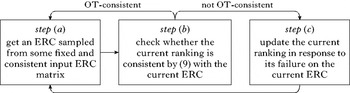
In many cases, we are interested in studying the behaviour of EDRAs irrespective of the proper definition of step (a) in Fig. 3, i.e. irrespective of the proper definition of the sub-routines that determine the underlying form and choose a loser form for the winner form the algorithm has been currently fed. In these cases, we can thus assume that the underlying and the loser forms are also provided to the algorithm, along with the winner form. In other words, we can assume that the algorithm is given as input at step (a) an underlying/winner/loser form data triplet, or, equivalently, the corresponding ERC. It is thus useful to restate EDRAs in terms of ERCs, as in Fig. 4. According to Fig. 4, the algorithm is trained on a stream of ERCs, and the current ranking is updated whenever it is inconsistent with the current ERC.
Main loop of an EDRA, restated in ERC notation.

Throughout this paper, I assume that the ERCs fed to the algorithm at step (a) are sampled from a fixed, given input ERC matrix, which I will assume to be consistent. As we will see in §4.3, this assumption can be made without loss of generality in certain applications, as in the case of modelling the acquisition of phonotactics.
2.3 Restatement in terms of ranking vectors
Boersma (Reference Boersma1997, Reference Boersma1998, Reference Boersma2009) points out that rankings can be represented numerically. To illustrate the idea, suppose we have three constraints discussed in §2.2, and let us pair them up with three numbers, as in (10). This triplet of numbers can be interpreted as follows: Fpos is top-ranked, because it corresponds to the largest number, M is bottom-ranked and Fgen is ranked in between.
(10)
In order for the correspondence in (10) to hold, it is crucial that the three numbers considered are all distinct. What if two of these numbers are identical? Consider for instance the case in (11), where the two constraints Fgen and M are assigned the same number. We can think of this triplet of numbers as simultaneously representing two different rankings, depending on how the tie between Fgen and M is resolved. We can think of these two rankings as two different ways of ‘refining’ the numerical tie.
(11)
These considerations allow OT grammars to be given a numerical parameterisation, besides the usual combinatorial parameterisation in terms of rankings. Here are the details.
A ranking vector is an n-tuple θ of numbers θ1, …, θn as in (12), one for each of the n constraints. The kth component θk is the ranking value (RV) of constraint Ck.
(12)
A ranking is a refinement of a ranking vector θ=(θ1, …, θn) provided condition (13) holds for any pair of constraints Ch, Ck. If the two RVs θh and θk tie, the antecedent of (13) fails, and different refinements can break the tie in either way. Otherwise, any refinement satisfies the ordering implicitly defined by the relative size of the two RVs θh and θk.
(13)
Once ranking vectors are paired up with rankings through (13), notions that pertain to rankings can be extended to ranking vectors. In particular, we can extend the notion of OT-consistency from rankings to ranking vectors. If a ranking vector admits a unique refinement, then the extension is straightforward: we will say that the ranking vector is consistent with an ERC provided its unique refinement is consistent with that ERC, according to the original notion of OT-consistency in (9). What if instead some of the RVs tie and the ranking vector thus admits multiple refinements? One option would be to declare the ranking vector consistent with an ERC provided at least one of its refinements is consistent with it, in the spirit of Anttila (Reference Anttila1997) and Anttila & Cho (Reference Anttila and Cho1998). At convergence, the algorithm will thus return a ranking vector that has the property that at least one of its refinements is consistent with the input ERC matrix. But this is not very useful: how do we decide for a given refinement whether it is what we want or not? Thus I will require consistency of every refinement in order to declare a ranking vector consistent with an ERC, as in (14).Footnote 3
(14) A ranking vector is (OT-)consistent with an ERC provided that each of its refinements is consistent with that ERC, according to the original notion of consistency (9).
For instance, the ranking vector in (10) is consistent with the ERC in (7), as the only refinement of the former is consistent with the latter. But the ranking vector in (11) is not consistent with (7), because of the inconsistent refinement Fpos≫M≫Fgen.
Boersma (Reference Boersma1997, Reference Boersma1998, Reference Boersma2009) suggests restating the EDRA in Fig. 4 in terms of ranking vectors, as in Fig. 5, the final formulation considered in this paper. The current hypothesis on the target grammar is stored by the algorithm as a numerical ranking vector, rather than as a combinatorial ranking. The current ranking vector is updated whenever it is found to be inconsistent with the current ERC.
Main loop of an EDRA, restated in terms of ranking vectors.

This restatement of EDRAs in terms of ranking vectors rather than rankings will prove to be crucial for the development of the theory of EDRAs' convergence.
2.4 Convergent re-ranking rules
Different EDRAs differ (mainly) because of the re-ranking rule used in step (c) of Fig. 5 in order to update the current ranking vector in response to its failure on the current ERC. This re-ranking operation can take various different forms. One option is to demote by a certain demotion amount certain loser-preferring constraints, as those are the constraints responsible for the failure of the current ranking vector on the current ERC. Another option is to promote by a certain promotion amount certain winner-preferring constraints, as those are the constraints that would have helped to avoid the failure of the current ranking vector on the current ERC. These two options are schematised in (15), which thus provides a general scheme for re-ranking rules.
- (15)
a. Subtract a certain demotion amount from the current RV of some or all of the loser-preferring constraints.
b. Add a certain promotion amount to the current RV of some or all of the winner-preferring constraints.
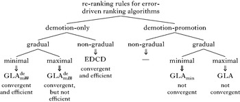
Re-ranking rules differ along three main dimensions. The first dimension is whether the re-ranking rule only performs constraint demotion or constraint promotion as well. The second dimension is whether the re-ranking rule minimally demotes only the loser-preferrers that need to be demoted or maximally demotes all of them. The third dimension is whether the re-ranking rule performs small, gradual updates or instead updates that are so ‘drastic’ that one update suffices to make the current ranking vector consistent with the current ERC, so that no ERC can trigger two consecutive updates. The re-ranking rules considered in the literature are classified in Fig. 6 according to these three dimensions, together with the name of the corresponding EDRA. §3 reviews what is currently known about re-ranking rules that perform constraint demotion only; §5 reviews what is currently known about re-ranking rules that perform both constraint demotion and promotion.
Taxonomy of the re-ranking rules considered in the literature.

An EDRA (with a specific re-ranking rule and a specific initial ranking vector) is said to converge on a given input ERC matrix provided that the algorithm can perform only a finite number of updates when trained on any stream of ERCs sampled from that ERC matrix. In other words, the algorithm always eventually settles on a ranking vector consistent with each input ERC, so that the algorithm cannot make any more errors, and learning ceases. An EDRA is (universally) convergent provided that it converges no matter what input ERC matrix it is trained on, as long as it is consistent. The restriction to consistent input ERCs makes good sense, as the EDRA could never converge on a consistent ranking otherwise. Furthermore, the restriction to consistent input ERCs can be enforced in some cases without loss of generality, as we will see in §4.3. A convergent EDRA is efficient provided that the number of errors made before convergence grows slowly (polynomially) with the number n of constraints, so that the algorithm also works in the case of very large constraint sets. For each of the main EDRAs considered in the literature, the synopsis in Fig. 6 indicates what is currently known concerning (universal) convergence and efficiency. In particular, it reveals that the ambitious requirement of efficient convergence can be achieved. The next section takes a close look at this result.
3 Tesar & Smolensky's analysis of demotion-only EDRAs
This section reviews the elegant analysis of demotion-only EDRAs developed in Tesar (Reference Tesar1995, Reference Tesar, Barbosa, Fox, Hagstrom, McGinnis and Pesetsky1998) and Tesar & Smolensky (Reference Tesar and Smolensky1996, Reference Tesar and Smolensky1998, Reference Tesar and Smolensky2000) (henceforth T&S).Footnote 4 T&S's analysis is important because it shows that efficient convergence can indeed be attained. Furthermore, T&S's analysis provides the starting point for the developments in the rest of this paper. My presentation of T&S's analysis owes a great deal to Prince's (Reference Prince2002) ERC notation. Furthermore, it underscores the benefit of framing the theory of EDRAs in terms of ranking vectors, rather than in terms of rankings, as in their original proposal.Footnote 5
3.1 A minimal, gradual demotion-only re-ranking rule
Consider the current ERC (16a) and the current ranking vector (16b). The two constraints C4 and C6 are both currently loser-preferrers. Yet there is a crucial difference between them. The current RV of C6 is 5, which is smaller than the current RV of the winner-preferrer C1. However, the current RV of C4 is 15, larger than the current RV of both winner-preferrers C1 and C2. This difference is important enough to warrant a name: a loser-preferrer is undominated if there is no winner-preferrer with a strictly larger current RV. Thus C4 is currently undominated, while C6 is not.
(16)
We can now consider the re-ranking rule (17), which demotes all undominated loser-preferrers by a small fixed amount, here set to 1 for concreteness.
- (17)
a. Decrease the RV of each undominated loser-preferrer by 1.
b. Do nothing to the current RV of the other constraints.
For instance, if the current ERC is (16a) and the current ranking vector is (16b), then the updated ranking vector is (18): the RV of the currently undominated loser-preferrer C4 is decreased by 1, from 15 to 14; all other RVs are left unchanged.
(18)
The re-ranking rule (17) is clearly demotion-only, as the current RVs of winner-preferrers are never modified. Furthermore, it is minimal, because it does not demote all loser-preferrers, but only those that really need to be demoted because they are not already ranked underneath a winner-preferrer, i.e. only the undominated ones. We will see in §3.6 why it is indeed a good idea to only demote the currently undominated loser-preferrers. Finally, (17) is gradual, in the sense that updates are performed by a small fixed amount, so that an ERC might have to trigger multiple consecutive updates before the current ranking vector becomes consistent with it. For instance, a single update of the current ranking vector (16b) by the ERC (16a) is not enough to enforce consistency with that ERC, as the updated ranking vector (18) is still not OT-consistent with it. As we will see in §3.7, it is easy to construct the non-gradual counterpart of a gradual re-ranking rule. The EDRA in Fig. 5, together with the re-ranking rule in (17), is Boersma's (Reference Boersma1997) (non-stochastic) minimal demotion-only Gradual Learning Algorithm.
3.2 The idea of the analysis
Suppose that the input ERC matrix is (19a) and the initial ranking values are all null. I provide in (19b) the complete learning paths described by the EDRA with the re-ranking rule (17). Suppose the algorithm receives ERC 1 at the first iteration. Since the initial ranking vector θ1 is not consistent with that ERC, the algorithm updates θ1 to θ2 by demoting the RV of the currently undominated loser-preferrer C2 by 1. As θ2 is now consistent with ERC 1, no further updates will be performed, until the algorithm is fed ERC 2. When that happens, θ2 is updated to θ3 by demoting by 1 the RV of the currently undominated loser-preferrer C3. And so on.
(19)
No matter the training sequence of ERCs, after three updates the algorithm entertains the ranking vector θ4, whose only refinement is the ranking C1≫C2≫C3. Since this ranking is consistent with both input ERCs, no further update will be triggered.
The input ERC matrix in (19a) is consistent only with the ranking in (20a), where stratum 1 is the top stratum.
(20)
The RV of C1 never goes below 0 in (19b), as stated in (20b). In fact, constraint C1 is never loser-preferring in the input ERC matrix, and is thus never demoted from its initial null RV. Furthermore, the RV of C2 never goes below −1. Indeed, C2 can only be demoted through update by ERC 1; in order for that ERC to trigger an update, C2 must be currently ranked above the winner-preferrer C1; since C1 is fixed at the RV θ1=0, this means that C2 can only be demoted when its current RV is θ2=0; therefore C2 can never be below θ2=−1. Finally, the RV of C3 never goes below −2. C3 can only be demoted through update by ERC 2; in order for that ERC to trigger an update, C3 must be currently ranked above the winner-preferrer C2; since C2 can only drop down to θ2=−1, this means that C3 can only be demoted when its current RV is θ3=0 or θ3=−1, therefore C3 can never go below θ3=−2.
Every time the EDRA makes an error on the current ERC, at least one constraint is demoted. Every time a constraint is demoted, its RV decreases by 1. Thus (20b) says that C1 can never be demoted, C2 can be demoted at most once and C3 at most twice. This means in turn that the EDRA can perform at most 0+1+2=3 errors. We have thus proved convergence on the simple input ERC matrix in (19a).
The conclusion obtained in (20) can be summarised as follows: the RV θk of the constraint Ck assigned to the stratum k (with stratum 1 being the top one) can never make it below −(k−1). This statement is called an invariant, as it is a property of the current RVs that holds at any iteration throughout learning. T&S note that this invariant holds in general, as explained in §3.4. The only requirement is consistency of the input ERC matrix, spelled out in §3.3. Efficient convergence then follows straightforwardly from this invariant, as will be shown in §3.5.
3.3 Characterisation of OT-consistency
T&S's analysis of convergence of demotion-only re-ranking rules (as well as the developments of that analysis presented in the rest of this paper) crucially relies on the assumption that convergence is at least in principle achievable, i.e. that the input ERC matrix is consistent with at least a ranking. In order to distil useful computational consequences from this assumption, we need explicit characterisations of OT-consistency. I present here the characterisation of OT-consistency developed by T&S, using the ERC notation of Prince (Reference Prince2002); I revisit the issue of the algorithmic implications of the notion of OT-consistency in Appendix C of the online supplementary materials.
To introduce the idea, consider the ERC matrix in (21a), which is consistent with the ranking C1≫C2≫C3≫C4≫C5. Reorder the columns of the matrix from left to right according to this ranking, as in (21b). Then place at the top ERCs a1 and a4, which have a w corresponding to C1, as in (21c). Below them place ERC a3, which has a w corresponding to C2, as in (21d).
(21)
The ERC matrix obtained in (21d) can be described as follows. There is a top block of rows whose first entry is w, and a second block (here just one row) whose first entry is e, followed by w. The first two entries of the rows in the third block are e, and are followed by w. A straightforward generalisation of the procedure illustrated in (21) yields the following characterisation of consistent ERC matrices.
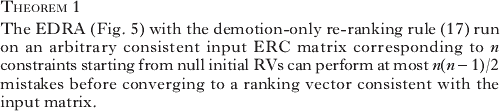
(22)
3.4 The crucial invariant
Consider a run of the EDRA with the demotion-only re-ranking rule (17) and initial null RVs. As the input ERC matrix is consistent, it can be brought into the form in (22), by Fact 1. The RV θ1 of constraint C 1 can never be as low as −1. Suppose by contradiction that it does. As C1 starts out at θ1=0, this means that C1 has been demoted at least once. But that is impossible, as the re-ranking rule (17) only demotes loser-preferrers, and C1 does not have a single l in (22). The RV θ2 of constraint C2 can never be as low as −2. Again, suppose by contradiction that it does. As the re-ranking rule (17) demotes by 1 only the undominated loser-preferrers, this means that at some point C2 had a current RV of θ2=−1 and was at that point an undominated loser-preferrer. But that is again impossible: in order for C2 to be loser-preferring, the current ERC must belong to block 1, in which case C2 is dominated by the winner-preferrer C1, as the RV of C2 is −1 by hypothesis, while the RV of C1 is always 0, as just shown. The cases of Ck with k>2 are dealt with analogously, by induction on k. We have thus proved the following crucial invariant.
(23)
3.5 Efficient convergence
Suppose that we could construct a consistent input ERC matrix on which the EDRA run with the demotion-only re-ranking rule (17) does not converge, but rather performs an infinite number of updates. This means in turn that some constraint is demoted an infinite number of times. Its RV thus becomes arbitrarily small, violating the lower-bound (23). Thus the algorithm needs to stop after a finite number T of updates. At each update, one or more demotions are performed. Thus the total number of updates T must be smaller than the total number of demotions, as stated in (24).
(24)
Without loss of generality, assume that the input ERC matrix is consistent with the ranking C1≫C2≫…≫Cn. Fact 2 says that C1 is never demoted, C2 is demoted at most once, C3 is demoted at most twice, and so on. Thus (24) becomes (25).
(25)
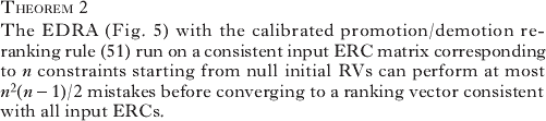
Using the identity 0+1+2+…+(n−1)=n(n−1)/2, we conclude with Theorem 1, which says that demotion-only converges efficiently, with a worst-case number of updates quadratic in the number n of constraints.
The bound n(n−1)/2 on the worst-case number of updates provided by the Theorem is tight, and thus not improvable. In fact, suppose that there are 4 constraints and that the input ERC matrix is (26a), which Riggle (Reference Riggle2009) calls ‘diagonal’. The learning path (26b) takes 4(4−1)/2=6 updates to reach convergence.
(26)
So far, I have only considered the case of null initial RVs. For the extension to arbitrary initial RVs, see Appendix A of the online supplementary materials.
3.6 Why only demote the loser-preferrers that are undominated?
The re-ranking rule (17) only demotes the loser-preferrers that really need to be demoted, namely the currently undominated ones, which are not currently ranked below a winner-preferrer. What happens if we demote all loser-preferrers, both the dominated and the undominated ones? For the sake of explicitness, consider the variant in (27). The EDRA in Fig. 5 with this re-ranking rule is Boersma's (Reference Boersma1997) (non-stochastic) demotion-only GLA.
- (27)
a. Decrease the RV of each loser-preferrer by 1.
b. Do nothing to the current RV of the winner-preferrers.
For instance, if the current ERC is again (16a) and the current ranking vector (16b), the updated ranking vector is (28): the RV of both loser-preferrers C4 and C6 is decreased by 1, despite the fact that only the former is currently undominated.
(28)
The invariant (23) says that constraints cannot be demoted too far, as long as we only demote the constraints that need to be demoted, namely the currently undominated loser-preferrers. This invariant no longer holds if all loser-preferrers, both dominated and undominated, are demoted. As a counterexample, consider the run in (29b), with the re-ranking rule (27): the RV of constraint C2 drops to −3, despite the fact that the input ERC matrix (29a) is consistent with the ranking C1≫C2≫C3≫C4, which assigns C2 to stratum 2.
(29)
In the case of the re-ranking rule (17), which demotes only currently undominated loser-preferrers, the invariant (23) entails efficient convergence, with an error-bound quadratic in the number of constraints. In the case of (27), which demotes all loser-preferrers, convergence still holds, but efficiency does not, as the worst-case number of errors can be shown to be exponential in the number of constraints; see Magri (Reference Magri2009). In conclusion, it is a good idea to demote only those loser-preferrers that need to be demoted, i.e. those that are currently undominated.
3.7 A non-gradual variant
The re-ranking rule in (17) is gradual, as it modifies the current RVs only by a small fixed amount. Thus multiple consecutive updates by a single ERC might be needed in order for the current ranking vector to become consistent with that ERC. For instance, the top path in (19b) shows that two consecutive updates by ERC 2 are needed before the current ranking vector becomes consistent with that ERC. Suppose that we wanted to save time, replacing those two updates with a single step. To achieve this, we would need to have demoted more the first time we encountered ERC 2, so that no further consecutive update by that ERC would have been necessary. A re-ranking rule is non-gradual provided it performs updates large enough that the current ranking vector becomes consistent with the current ERC after a single update, so that no ERC can trigger two consecutive updates. To illustrate, consider re-ranking rule (30), which demotes currently undominated loser-preferrers to a position below the currently top-ranked winner-preferrer. The EDRA in Fig. 5 with this re-ranking rule is T&S's EDCD.Footnote 6
- (30)
a. Decrease the current RV of each undominated loser-preferrer to θ* – 1, where θ* is the largest RV over winner-preferrers.
b. Do nothing to the current RV of the other constraints.
For instance, if the current ERC is again (16a) and the current ranking vector (16b), the updated ranking vector is (31). Only the RV of C4 is modified, as it is the only currently undominated loser-preferrer. It is decreased from its original value 15 to the updated value 9, i.e. the RV θ*=10 of the currently top-ranked winner-preferrer C1 further decreased by 1.
(31)
The undominated loser-preferrer C 4 is demoted in (31) by 6. This amount is large enough that the updated ranking vector is consistent with the ERC after just one update. Re-ranking rule (30) is non-gradual, because no ERC can trigger two consecutive updates. This non-gradual rule is a ‘speeded up’ version of the gradual re-ranking rule in (17). Thus it comes as no surprise that the analysis developed above for (17) extends to (30), ensuring efficient convergence in the latter case as well.
3.8 Summary
In this section, we have seen that efficient convergence is possible, at least in the case of EDRAs that only perform constraint demotion. The core of the analysis can be summarised as follows: every time the algorithm performs an update, some RVs are decreased; yet RVs cannot be decreased too much, because of the invariant (23); thus the algorithm cannot make too many updates. Furthermore, we have seen two rules of thumb for devising good re-ranking rules. First, not all loser-preferrers should be demoted, but only those that really need to be, the currently undominated ones. Second, we can focus on gradual re-ranking rules, as non-gradual convergent re-ranking rules can then be obtained straightforwardly from gradual ones, by collapsing multiple updates by the same ERC.
4 Some constraint promotion is needed too
In the preceding section, we looked at re-ranking rules from a purely computational perspective. In particular, we focused on re-ranking rules that perform constraint demotion but no constraint promotion. We saw that they have remarkable computational properties, as the corresponding EDRA efficiently convergences for any consistent input ERC matrix. In this section, we look at re-ranking rules from a modelling perspective: is demotion-only enough from a modelling perspective, or is some constraint promotion needed too? This issue has been addressed so far only marginally in the OT literature. Fikkert & de Hoop (Reference Fikkert and de Hoop2009: 311) raise the question, but dismiss the issue, suggesting that ‘in practice, the two approaches [constraint promotion and constraint demotion] are highly similar’ (2009: 319). Gnanadesikan (Reference Gnanadesikan2004: 73) endorses constraint promotion: ‘the process of acquisition is one of promoting the faithfulness constraints to approximate more and more closely the adult grammar, and produce more and more marked forms’. But she does not provide arguments in support of constraint promotion, nor does she provide an explicit re-ranking rule. Bernhardt & Stemberger (Reference Bernhardt and Stemberger1998), Stemberger & Bernhardt (Reference Stemberger, Bernhardt and MacWhinney1999, Reference Stemberger and Bernhardt2001) and Stemberger et al. (Reference Stemberger, Bernhardt and Johnson1999) argue in favour of constraint promotion for some specific cases, but are not computationally explicit. Boersma (Reference Boersma1997, Reference Boersma1998) and Boersma & Hayes (Reference Boersma and Hayes2001) provide the first computationally explicit argument in favour of constraint promotion, arguing that demotion-only is unable to model certain cases of language variation. This argument is framed within a stochastic variant of the traditional OT framework considered in this paper. In this section, I contribute to this debate a new explicit argument in favour of constraint promotion. I argue that demotion-only is insufficient for one of the most important modelling applications of EDRAs, namely modelling the early stage of the acquisition of phonotactics by the child.
4.1 Modelling the early stage of the acquisition of phonotactics
In carefully controlled experimental conditions, nine-month-old infants already react differently to licit and illicit sound combinations (Jusczyk et al. 1993, among others). They thus display knowledge of phonotactics at an early stage, when other linguistic abilities are still not fully developed. In particular, morphology is still lagging behind at this early age, so that the child still has no access to phonological alternations. Hayes (Reference Hayes2004: 165) thus concludes that ‘it seems a reasonable guess that in general, the learning of patterns of alternation [that only comes with knowledge of morphology] lags behind the learning of the contrast and phonotactic systems’. In other words, there is a developmental stage, the early stage of the acquisition of phonotactics, throughout which the child acquires phonotactics without the aid of phonological alternations.
Another crucial property of the acquisition of phonotactics is gradualness: the target adult grammar is approached through a path of intermediate stages (for classical examples, see e.g. Smit et al. Reference Smit, Hand, Freilinger, Bernthal and Bird1990, Levelt et al. Reference Levelt, Schiller and Levelt2000, Pater & Barlow Reference Pater and Barlow2003 and Gnanadesikan Reference Gnanadesikan2004; for reviews, see e.g. McLeod et al. Reference McLeod, Doorn and Reed2001 and Zamuner et al. Reference Zamuner, Gerken and Hammond2005). Assume that this gradualness reflects grammatical development, rather than just the slow development of performance factors that are orthogonal to linguistic competence (say the slow development of the articulators and of the corresponding motor programs); see Smolensky (Reference Smolensky1996a), as well as Hale & Reiss (Reference Hale and Reiss1998) for critical discussion. From this perspective, EDRAs provide an ideal model of the acquisition of phonotactics, as they describe a path within the space of possible phonotactics that can be matched with attested acquisition paths. What should a proper error-driven ranking model of the early stage of the acquisition of phonotactics look like?
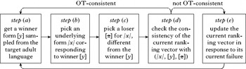
To address this question, consider the full-blown description of EDRAs in Fig. 7. The algorithm maintains a current ranking vector, initialises it to an assigned initial ranking vector and keeps updating it by looping through the five steps (a)–(e). At step (a), the algorithm receives a form [y] from the target adult language. At step (b), the algorithm needs to apply some subroutine in order to figure out a corresponding underlying form /x/. And at step (c), it needs to choose a corresponding loser form [z] (up to now, I have collapsed these three steps into a single one, as the focus was on the computational rather than the modelling side). At step (d), the algorithm checks whether the current ranking vector is consistent with the underlying/winner/loser form triplet (/x/, [y], [z]) thus assembled. If it isn't, then it takes action at step (e).
Full-blown description of the main loop of an EDRA.

Various implementation details now need to be specified, concerning the choice of the initial ranking vector, the subroutine that provides the underlying form /x/ at step (b) and the re-ranking rule to be used at step (e).Footnote 7 I discuss these three issues in turn in §§4.2–4.4. The conclusion of the argument will be that constraint promotion is crucially needed in order to turn the algorithmic kernel in Fig. 7 into a proper model of the early stage of the child acquisition of phonotactics.
4.2 Choice of the initial ranking vector
There is wide agreement in the literature that markedness constraints should start out initially ranked above faithfulness constraints; see Smolensky (Reference Smolensky1996a, b) for theoretical arguments in favour of this hypothesis, Jusczyk et al. (Reference Jusczyk, Smolensky and Allocco2002) for empirical evidence, Davidson et al. (Reference Davidson, Jusczyk and Smolensky2004) for a review and Hale & Reiss (Reference Hale and Reiss1998) for critical discussion. I thus assume that the initial RV of markedness constraints is larger than that of faithfulness constraints. For instance, assume that the former is some large positive constant θinit>0, while the latter is zero.
4.3 Choice of the underlying form
At step (a), the EDRA is fed a licit surface form [y] from the target adult language and needs to pick a proper corresponding underlying form /x/ at step (b), as well as a loser form [z] at step (c). To see how to proceed, consider a concrete example. Suppose the learner is provided with the winner form [y]=[rat]. To keep things simple, suppose the only option for the loser is [z]=[rad], and that there are two options for the underlying form: the learner could select the underlying form /x/=/rat/, faithful to the winner, and thus construct the triplet (32a), or it could select the underlying form /x/=/rad/, unfaithful to the winner, and thus construct the triplet (32b).
(32)
The choice of the non-faithful underlying form in the data triplet (32b) is equivalent to the assumption that the target phonology enforces final devoicing. But this assumption might be dangerous. In fact, a crucial property of the early stage of the acquisition of phonotactics is that the learner is still blind to alternations, as noted above. At this stage, the learner is thus not in a position to evaluate its assumption that the target phonology enforces final devoicing. The choice of a non-faithful underlying form might thus turn out to fool the learner into positing inconsistent data triplets at steps (a)–(c) of Fig. 7. I thus assume that the learner posits an underlying form faithful to the winner, as illustrated in the triplet (32a) and stated in (33). This assumption models the fact that the child is blind to alternations throughout the early stage of the acquisition of phonotactics; see Hayes (Reference Hayes2004) and Prince & Tesar (Reference Prince and Tesar2004).
(33) At step (b), the EDRA posits an underlying form /x/ identical to the given surface form [y], thus always building faithful triplets such as (32a).
Of course, this assumption only makes sense provided that the set of underlying forms coincides with the set of surface forms, so that the same phonological structure can be construed both as an underlying and as a surface form. In that case, a result by Tesar (Reference Tesar2008) shows that assumption (33) has a remarkable computational property: the underlying/winner/loser form triplets thus constructed at steps (a)–(c) are always consistent, under only mild assumptions on the constraint set. Tesar's result means in particular that, at least in the case of the acquisition of phonotactics, OT-consistency of the data fed to the algorithm can be assumed without loss of generality.
4.4 Choice of the re-ranking rule
We are now left with the crucial choice of the re-ranking rule that a proper error-driven ranking model of the early stage of the acquisition of phonotactics should use at step (e) of Fig. 7. From a computational perspective, a crucial issue that bears on the choice of the re-ranking rule is that of efficient convergence: which choices ensure that the number of errors is finite and grows slowly with the number of constraints? Suppose that the EDRA indeed converges. Then its final grammar successfully rules in every licit form – otherwise the algorithm could still make mistakes, and therefore could not have converged. Yet phonotactics is the knowledge of the distinction between licit and illicit forms. If, say, the final grammar ranks all faithfulness constraints at the top, then it fails to rule out any illicit form, and the EDRA has effectively learned nothing. A second issue relevant to the choice of the re-ranking rule to be used at step (e) is thus that of restrictiveness: which choices ensure that the final grammar entertained by the EDRA at convergence successfully manages to rule out illicit forms? Finally, suppose that the EDRA converges to a restrictive final grammar. On its way to that grammar, the EDRA entertains a path of intermediate rankings, each corresponding to an intermediate OT phonotactics. Thus the third issue is that of matching: which choices yield learning sequences that best match attested acquisition paths?
The focus of this paper is squarely on the first of these three issues, namely efficient convergence. As reviewed in §3, demotion-only re-ranking rules fare well from the computational perspective of convergence. However, in this subsection I will take a detour from my main focus on convergence, and look at the choice of the re-ranking rule from the modelling perspective of restrictiveness and matching between predicted learning sequences and acquisition paths. I will argue that, from the latter perspective, demotion-only is insufficient and that some degree of constraint promotion is needed. This conclusion will motivate the rest of the paper, which develops provably convergent re-ranking rules that perform both constraint demotion and promotion.
4.4.1 Choice of the re-ranking rule from the perspective of child acquisition paths
Suppose that the EDRA uses a re-ranking rule at step (e) that performs constraint demotion but no constraint promotion, like re-ranking rules (17) and (30). By (33), the algorithm posits underlying forms at step (b) that are fully faithful to the intended winners. Thus the faithfulness constraints are never loser-preferring. As demotion-only re-ranking rules only re-rank loser-preferrers, the model will never re-rank the faithfulness constraints throughout learning. This means in turn that the model predicts learning sequences where the repair strategy for a given marked structure never changes over time, as the choice of the repair strategy is determined by the relative ranking of the faithfulness constraints. This cannot be right, as acquisition paths do show changes in repair strategies over time. A certain amount of constraint promotion is thus needed in order for the model to have a chance to match child acquisition paths. Let me make this point explicit with some examples.
English-learning children go through various intermediate learning stages where they reduce licit onset consonant clusters to a singleton consonant. Crucially, the strategies used to determine the singleton consonant vary over time. Based on a large review of the literature, McLeod et al. (Reference McLeod, Doorn and Reed2001) show that child cluster simplification typically starts out as deletion of one of the two consonants, and that deletion is replaced at a subsequent stage by coalescence of the two target consonants into a singleton consonant, at least for certain targets. These learning dynamics crucially require re-ranking of the two faithfulness constraints Max (which militates against consonant deletion) and Uniformity (which militates against consonant coalescence). By (33), the EDRA will be trained on faithful underlying/winner/loser form triplets such as (/kl/, [kl], [k]) or (/s1m2/, [s1m2], [f1,2]). Thus neither Max nor Uniformity will ever be loser-preferring constraints, and neither of them will ever be re-ranked by demotion-only re-ranking rules, as these rules only re-rank the loser-preferrers. The demotion-only EDRA is thus unable to model even the very rough outline of the acquisition path towards English consonant clusters.
The same point can be made by looking at different acquisition stages adopted by different children. Pater & Barlow (Reference Pater and Barlow2003) review production data from two children, Gitanjali (age 2:3–2:9; Gnanadesikan Reference Gnanadesikan2004) and Julia (age 1:7–1:9; Compton & Streeter Reference Compton and Streeter1977). The two children display different patterns of coalescence for targets consisting of a stop+approximant. Julia preserves the continuancy of the approximant (e.g. [fɪm] ‘cream’), while Gitanjali preserves the continuancy of the stop (e.g. [pait] ‘quite’). Pater & Barlow model the two different coalescence patterns, assuming that Julia is currently ranking Ident[+cont] above Ident[−cont], while Gitanjali has the opposite ranking. Assume that the two children start from the same initial ranking vector, i.e. that UG has a built-in initialisation step. By (33), the EDRA assumes underlying forms faithful to the winner. If it performs demotion-only, it will never re-rank the two faithfulness constraints throughout learning, and will thus be unable to explain how the two children currently have two different rankings of the constraints.
4.4.2 Choice of the re-ranking rule from the perspective of restrictiveness
Assume that the EDRA adopts a demotion-only re-ranking rule, and thus only re-ranks loser-preferring constraints. Furthermore, assume by (33) that it posits underlying forms faithful to the winner, so that the faithfulness constraints are never loser-preferrers. Thus the EDRA will never re-rank the faithfulness constraints. As just seen, this cannot be right from the perspective of modelling acquisition paths. Let me now argue that it also cannot be right from the perspective of restrictiveness. In fact, if the faithfulness constraints are never re-ranked through learning, their final relative ranking is insensitive to the language the algorithm has been trained on. Suppose that restrictiveness requires the opposite relative ranking of some faithfulness constraints for a certain pair of languages in the OT typology. A demotion-only EDRA that posits faithful underlying forms will not re-rank the faithfulness constraints, and will thus be unable to learn the different rankings needed for the two languages. Some constraint promotion is needed in order to re-rank the faithfulness constraints too, despite the fact that they are never loser-preferrers.
These considerations can be illustrated with (34), which is a simplified version of an example considered in Prince & Tesar (Reference Prince and Tesar2004), based on Lombardi (Reference Lombardi1999). The [stop-voicing] and [fricative-voicing] features come with specific faithfulness and markedness constraints, F1, M1 and F2, M2. The markedness constraint M3, which requires adjacent obstruents to agree in voicing, allows the two features to interact. The generating function only modifies voicing.
(34)
Among the languages in the OT typology in (34), there are the two in (35).
(35)
A ranking generates these two languages, provided it is a refinement of the partial orders in (36a) and (36b) respectively. Consider for instance the language in (35a). In order for /ba/ not to be neutralised to [pa], the ranking (36a.i) is needed. In order for /za/ to be neutralised to [sa], the ranking (36a.ii) is needed. Given ranking (36a.ii), in order for /abza/ not to be neutralised to [apsa], we need the ranking (36a.iii), and, in order for /abza/ not to be neutralised to [absa], the ranking (36a.iv) is needed too.
(36)
Because of the assumption that underlying forms are fully faithful to the intended winners (33), the two faithfulness constraints F1 and F2 are never loser-preferring. If the EDRA in Fig. 7 is implemented with a demotion-only re-ranking rule that only demotes loser-preferrers, such as (17) or (30), then the two faithfulness constraints F1 and F2 will retain their initial RVs. In other words, the final relative ranking of F1 and F2 will be the same, no matter which of the two languages in (35) the algorithm is trained on. The algorithm will thus fail to acquire the phonotactics of at least one of the two languages, as they require the opposite relative ranking of F1 and F2, by (36). These considerations show that constraint promotion is a necessary condition in order for EDRAs to provide a proper model of the early stage of the acquisition of phonotactics, as promotion also allows the faithfulness constraints to be re-ranked throughout learning, despite the fact that they are never loser-preferrers.Footnote 8
4.4.3 More on restrictiveness and constraint promotion
What happens when an EDRA that performs both constraint demotion and promotion is trained on the two languages in (35)? Is it indeed able to rank the faithfulness constraints correctly, as in the target rankings in (36)? The input ERC matrices corresponding to (35) are provided in (37). Let me explain how matrix (37a), for instance, has been computed. The target language consists of the five surface forms [pa], [ba], [sa], [apsa] and [abza]. Of these five forms, only [ba] and [abza] are informative, as the other three forms are unmarked, and therefore do not contribute to learning (their ERCs never trigger any updates). For the informative form [ba], we need to consider only one underlying/winner/loser triplet, namely the one that pairs this winner surface form with the faithful underlying form /ba/ and the loser form [pa]. For the other informative form, [abza], we need to consider three triplets, which pair this winning form with the faithful underlying form /abza/ and the three loser forms [apsa], [apza] and [absa]. The ERC matrix in (37a) is obtained by assembling, one on top of the other, the ERCs corresponding to these four triplets.
(37)
I provide in Fig. 8 the dynamics of the RVs of the five constraints predicted by the EDRA with a promotion-demotion re-ranking rule trained on the two input matrices in (37). The initial ranking vector used in the simulations has been chosen according to §4.2: the faithfulness constraints are initially ranked at the bottom (with a null initial RV) and the markedness constraints at the top (with an initial RV of θinit=10000). The simulations use the (efficiently convergent) re-ranking rule (51) developed below in §6: the details of the re-ranking do not matter here, except for the fact that constraint promotion is performed as well as demotion. Finally, the ERCs are sampled uniformly from the input ERC matrix.

The final ranking vectors that the promotion/demotion EDRA converges to in the two simulations in Fig. 8 are provided in (38a) and (b) respectively.
(38)
Surprisingly, these two final ranking vectors correctly represent the two target rankings in (36). Consider for instance (38a): the RV of F1 is larger than both the RVs of M1 and M2, thus representing the target rankings (36a.i) and (36a.iii), the RV of M2 is larger than the RV of F2 (36a.ii) and the RV of M3 is larger than the RV of M2 (36a.iv). In particular, the promotion component of the re-ranking rule has allowed the EDRA to learn the correct relative ranking of the two faithfulness constraints F1 and F2.
A quick look at the input ERC matrices in (37) reveals what is behind this success. Consider for instance (37a). The three markedness constraints start out with the same initial RV. After one update by the penultimate ERC, M1 is demoted and M3 is promoted. The current ranking vector thus enforces the ranking configuration M3≫M1, ensuring consistency with this ERC. Furthermore, this ranking configuration will never be disrupted in the rest of the learning process, as M3 can never be demoted (because it is never a loser-preferrer) and M1 can never be promoted (because it is never a winner-preferrer). Thus the penultimate ERC can trigger at most one update, and is therefore pretty much irrelevant for the overall ranking dynamics. Analogous considerations hold for the last ERC, so that the ranking dynamics are completely determined by the first two ERCs. The first ERC promotes only F1, while the second ERC promotes both F1 and F2. Thus a single update by the first ERC is sufficient to ensure that F1 will be ranked above F2 from that time on. In other words, a single update by the first ERC is enough to guarantee that the EDRA will converge to the correct relative ranking of the two faithfulness constraints. As F1 is thus ranked above F2, the two markedness constraints M1 and M2 will intercept F1 first in their free fall. As soon as they cross F1, learning ceases, as the current ranking vector has become consistent with the entire ERC matrix. M1 and M2 thus find themselves squeezed in between F1 and F2, as desired. Although the input ERCs are sampled uniformly in the simulations reported above, the analysis just sketched reveals that the EDRA will converge to the correct final ranking no matter how the input ERCs are sampled, as long as the first ERC gets a chance to trigger a few updates. In conclusion, the OT typology in (34) has the following remarkable property: the only two languages that require a faithfulness constraint to be ranked above another faithfulness constraint correspond to input ERC matrices that are able to train the EDRA to learn that relative ranking.
In Magri (Reference Magri2012b), I show that EDRAs are restrictive on any language that does not require any faithfulness constraint to be ranked above another faithfulness constraint. As expected, such languages constitute the vast majority: the relative ranking of the faithfulness constraints matters for the way illicit structures are repaired, but it matters only rarely for the divide between licit and illicit structures. What about the remaining languages, which require a specific relative ranking of the faithfulness constraints? In Magri (Reference Magri, Heinz, Cahill and Wicentowski2010, to appear a), I show that restrictiveness cannot be achieved in the general case by any algorithmic scheme. In other words, there is no learning algorithm from positive evidence that can ensure restrictiveness, unless we make assumptions about the underlying OT typologies. This result motivates the following conjecture: is it the case that phonologically plausible OT typologies happen to have the property just observed for the typology in (34), i.e. that every language in the typology that requires a certain faithfulness constraint to be ranked above another faithfulness constraint correspond to an input ERC matrix that is able to train the EDRA to learn that relative ranking? If this conjecture turns out to be correct, it will provide formidable support for the hypothesis that error-driven learning is a proper model of the child's acquisition of phonotactics. In Magri (Reference Magri, Carlson, Hölscher and Shipley2011, Reference Magri2012b), I report a first result in this direction. I consider all possible constraints of the type of M3 in (34), which is responsible for the interaction between the two features that define the typology. And I show that promotion/demotion EDRAs are restrictive, except for phonologically implausible models of feature interaction.
4.5 Summary
Tesar & Smolensky (Reference Tesar and Smolensky1998) develop the first EDRA, error-driven constraint demotion, reviewed in §3. Its signature property is that it performs constraint demotion but no constraint promotion. Lack of constraint promotion allows Tesar & Smolensky to prove that EDCD converges with an efficient error-bound (cf. also Boersma Reference Boersma2009). Although a virtue from a computational perspective, lack of constraint promotion turns out to be a liability from a modelling perspective, as argued in this section. I have looked at one of the main modelling applications of EDRAs, the modelling of the early stages of the acquisition of phonotactics. In this case, it makes sense to assume that the EDRA is provided with winner forms only, and that it assumes underlying forms faithful to the winners. Training on faithful mappings entails that faithfulness constraints are never loser-preferrers. As EDCD only demotes loser-preferrers, it never re-ranks the faithfulness constraints. This cannot be right from the perspective of restrictiveness: if two languages in the typology require the opposite relative ranking of some faithfulness constraints, EDCD fails to learn that. Furthermore, it cannot be right from the perspective of matching the predicted learning sequences with acquisition paths: if an acquisition path shows a succession of different repair strategies for the same marked structure, EDCD fails to model it. In conclusion, EDCD is unable to implement the error-driven learning model of the acquisition of phonotactics. And some amount of constraint promotion is needed, in order to re-rank the faithfulness constraints, despite the fact that they are never loser-preferrers. This conclusion motivates the research question addressed in the rest of this paper: is it possible to devise convergent re-ranking rules that perform constraint promotion in addition to demotion? §5 reviews what is currently known in the OT computational literature concerning constraint promotion.
5 The computational challenge raised by constraint promotion
In this section, I illustrate the computational challenge raised by constraint promotion, with a review of the unsuccessful attempts at constraint promotion made so far in the literature.
5.1 The credit problem
Suppose that the current ERC fed to the EDRA has multiple w's; say it has two w's corresponding to the two constraints Ch and Ck, as in (39a). A promotion/demotion EDRA needs to decide which one of the two winner-preferrers, Ch or Ck, should be credited for OT-consistency with the current ERC. And the decision must be taken instantaneously, without looking at the rest of the ERC matrix. This is a very challenging task. In fact, the ERC matrix could contain another ERC like (39b), which says that only Ch should be credited for shielding the loser-preferrer of the ERC in (39a). This is an example of what Dresher (Reference Dresher1999) calls the ‘credit problem’.
(39)
A demotion-only re-ranking rule gets around the credit problem by avoiding any promotion. But a promotion/demotion re-ranking rule might in principle be fooled by the credit problem, as noted by Tesar & Smolensky (Reference Tesar and Smolensky1998: 244), who explicitly warn against constraint promotion: according to EDCD, ‘all movement of constraints is downward in the hierarchy. One could reasonably ask … couldn't the learner just as easily promote constraints toward the correct hierarchy? The answer is no’.
5.2 Gradualness and the credit problem
Boersma (Reference Boersma1997, Reference Boersma1998) suggests that gradualness might get around the credit problem. Consider a re-ranking rule that makes only small, gradual adjustments at each iteration. Even if at a given iteration the algorithm incorrectly promotes a winner-preferrer that should in the end be at the bottom of the ranking, this will be only a small mistake, and small mistakes will hopefully in the end be overridden by subsequent better moves.
More explicitly, Boersma (Reference Boersma1997, Reference Boersma1998) and Boersma & Hayes (Reference Boersma and Hayes2001) consider the re-ranking rule in (40), whereby loser-preferrers are demoted and winner-preferrers promoted by a small amount, say 1. This is the only example in the current literature of a re-ranking rule that performs both constraint demotion and promotion. The EDRA in Fig. 5 with this re-ranking rule is Boersma's (Reference Boersma1997) (non-stochastic) Gradual Learning Algorithm.Footnote 9
- (40)
a. Decrease the RV of each loser-preferrer by 1.
b. Increase the RV of each winner-preferrer by 1.
For instance, if the current ERC and the current ranking vector are again as in (16), then the updated ranking vector is (41). The RVs of the two loser-preferrers C4 and C6 are decreased from 15 and 5 to 14 and 4. And the RVs of the two winner-preferrers C1 and C2 are increased from 10 and 5 to 11 and 6.
(41)
The GLA converges in the case of input ERC matrices that have a unique winner-preferrer per ERC, and thus do not raise any credit problem.Footnote 10 But what about the case of input ERC matrices with multiple winner-preferrers per ERC? Does Boersma & Hayes' conjecture above, that gradualness gets around the credit problem, prove correct? As observed by Keller & Asudeh (Reference Keller and Asudeh2002), this question remained open for a number of years, until Pater (Reference Pater2008) showed that gradual promotion/demotion re-ranking rules are also indeed fooled by the credit problem, despite the fact that they make only small adjustments to the current RVs. He considers the input ERC matrix (42), which exacerbates the credit problem by stacking multiple ERCs with two winner-preferrers. He reports that the GLA trained on this input ERC matrix (with the ERCs sampled uniformly and with identical initial RVs for the five constraints) keeps increasing its current RVs, without ever converging to an consistent vector.Footnote 11 Pater's counterexample thus settles the issue of the convergence of the GLA.Footnote 12
(42)
Pater does not explain why exactly the specific instance of the credit problem raised by his counterexample fools the GLA. Furthermore, he leaves it open whether the GLA might converge if the strong regularity of the ERC matrix (42) is broken by sampling its rows according to a skewed distribution, rather than the uniform distribution considered in his simulations. In §5.3, I offer a detailed explanation of the failure of the GLA on Pater's counterexample: the algorithm fails because all ranking vectors consistent with the input ERC matrix lie outside its search space. This explanation shows in particular that the GLA fails no matter how the ERCs in (42) are sampled and fed to the algorithm, thus slightly strengthening Pater's counterexample.
5.3 A detailed explanation of Pater's counterexample
Consider a run of the GLA on Pater's counterexample (42), starting from null initial RVs. Every time ERC 1 triggers an update according to (40), the RVs of the winner-preferrers C1 and C3 are increased by 1, and the RV of the loser-preferrer C2 is decreased by 1. Equivalently, the current ranking vector is updated by adding to it the update vector corresponding to ERC 1, i.e. the vector that has a 1 for the two winner-preferrers C1 and C3, −1 for the loser-preferrer C2 and 0 elsewhere. Every time ERC 2 triggers an update according to (40), the RVs of the winner-preferrers C2 and C4 are increased by 1, and the RV of the loser-preferrer C3 is decreased by 1. Equivalently, the current ranking vector is updated by adding to it the update vector corresponding to ERC 2, which has a 1 for the two winner-preferrers C2 and C4, −1 for the loser-preferrer C3 and 0 elsewhere. And so on.
Thus the ranking vector θ entertained by the GLA at a generic iteration has the shape in (43): it is obtained by adding together the four column vectors that appear in (43), each multiplied by a non-negative coefficient αi. The ith column vector in (43) is the update vector corresponding to the ith ERC of Pater's counterexample (42). It is obtained by replacing each w, l and e in the ERC with 1, −1 and 0 respectively, thus encoding the contribution of the ith ERC to the current ranking vector according to the GLA re-ranking rule in (40). The corresponding coefficient αi in (43) represents the number of updates triggered by the ith ERC of Pater's tableau in the run up to the time considered.
(43)
Adding up the corresponding components in (43), we can conclude that the search space of the GLA run on Pater's counterexample, starting from the null initial vector, is a subset of the set of ranking vectors of the form (44), for non-negative coefficients α1, α2, α3, α4. This conclusion makes good sense. Constraint C1 starts out with a null initial RV and is promoted by 1 every time ERC 1 triggers an update. Thus the current RV θ1 of constraint C1 must always be equal to the number α1 of updates triggered by ERC 1, as stated in the first equation in (44). Constraint C2 starts out with a null initial RV, is promoted by 1 every time ERC 2 triggers an update and demoted by 1 every time ERC 1 triggers an update. Thus the current RV θ2 of constraint C2 must always be equal to the number α2 of updates triggered by ERC 2 minus the number α1 of updates triggered by ERC 1, as stated in the second equation in (44). And so on.
(44)
There is only one ranking consistent with the ERC matrix in (42), namely C1≫C2≫C3≫C4≫C5. Thus, a ranking vector θ=(θ1, θ2, θ3, θ4, θ5) is consistent with Pater's ERC matrix only if it univocally represents this ranking, i.e. it satisfies the four strict inequalities θ1>θ2>θ3>θ4>θ5. By virtue of the characterisation in (44) of the ranking vectors entertained by the GLA, these four strict inequalities can be rewritten as the four strict inequalities in (45), in terms of the coefficients α1, α2, α3, α4.
(45)
Crucially, the four strict inequalities in (45) are not feasible, as there exist no coefficients α1, α2, α3, α4 that satisfy all four of them at the same time (see Appendix E of the online supplementary materials). In conclusion, the reason why the GLA fails on Pater's counterexample is as follows: the search space of the GLA is limited to ranking vectors of the form (44), but no such ranking vector is consistent with Pater's ERC matrix, as none satisfies the inequalities in (45). In other words, the GLA fails because it struggles to reach a ranking vector that lies beyond its reach.Footnote 13 Pater detected the failure of the GLA on (42) through simulations where the various ERCs were sampled uniformly. The explanation just provided slightly strengthens his counterexample, showing that the GLA fails no matter how the input ERCs are sampled and fed to the algorithm.
5.4 Summary
On the one hand, §4 argued in favour of constraint promotion from a modelling perspective: throughout the early stage of the acquisition of phonotactics, the learner can confidently only posit underlying forms faithful to the winners; the faithfulness constraints would therefore never be re-ranked by a demotion-only EDRA, as they are never loser-preferrers; and the predicted learning dynamics would thus be too simple to match the attested typological and acquisition complexity. On the other hand, this section has shown that constraint promotion is hard to devise from a computational perspective, because of the credit problem: only a subset of the current winner-preferrers should be credited for accounting for the current loser-preferrers; it is not possible to promote only these useful winner-preferrers, because we cannot select them based only on the current ERC, and it is not safe to promote all of them, because this strategy leads to repeated promotions of winner-preferrers that should be low-ranked, as in Pater's counterexample. The rest of the paper presents a solution to this impasse, allowing us to move a step forward towards the integration of the modelling and computational perspectives.
6 Calibration of the promotion amount ensures efficient convergence
§3.6 showed that faster convergence is achieved by demoting only the loser-preferrers that need to be demoted, i.e. the currently undominated ones, rather than all of the loser-preferrers. Let the demotion amount by which the undominated loser-preferrers are demoted be a small, fixed amount, say 1 for concreteness. The demotion component of the re-ranking rule thus looks like (46a). Let the promotion amount be the small amount by which the winner-preferrers are promoted, which I will denote by p, as in (46b).
- (46)
a. Decrease the RV of each undominated loser-preferrer by 1.
b. Increase the RV of each winner-preferrer by p.
The demotion-only re-ranking rule in (17) corresponds to (46), with a null p=0 promotion amount. Lack of constraint promotion allowed T&S to prove convergence after a worst-case number of errors that grows only quadratically in the number of constraints, as reviewed in §3. Boersma's (Reference Boersma1997) GLA re-ranking rule in (40) corresponds to (46), with p=1.Footnote 14 The addition of this promotion component disrupts the good convergent behaviour of demotion-only, as shown by Pater's (Reference Pater2008) counterexample reviewed in §5.
The first three ERCs of Pater's matrix in (42) have two winner-preferrers and one loser-preferrer. The GLA demotes the loser-preferrer by 1 and promotes each of the two winner-preferrers by 1. Overall, the GLA thus demotes by 1 (as it demotes once), but promotes by 2 (as it promotes twice). In other words, the GLA performs overall more promotion than demotion. As the promotion component of the update overwhelms the demotion component, the good convergent behaviour of demotion-only is disrupted. But what if the promotion component (46b) of the re-ranking rule is properly calibrated, so that it never overwhelms the demotion component (46a)? Is the good convergence behaviour of demotion-only retained in this case? And how should the promotion amount p be chosen?
The rest of this paper provides a complete answer to these questions. Let us say that a re-ranking rule of the form (46) is calibrated provided that the promotion amount p is chosen in such a way that the promotion component of the re-ranking rule never overwhelms the demotion component. §6.1 shows that calibration holds provided the promotion amount p is strictly smaller than the crucial threshold l/w, namely the ratio between the number l of currently undominated loser-preferrers and the number w of winner-preferrers. §§6.2–6.4 then demonstrate that a slight extension of T&S's analysis shows that calibration is a sufficient condition for efficient convergence. For instance, set the promotion amount equal to p=l/(w+1), which is calibrated, as it is slightly smaller than the calibration threshold l/w. The corresponding EDRA converges after a worst-case number of errors that grows only cubically with the number of constraints. This bound compares well with the quadratic error-bound obtained by T&S for demotion-only. §7 will then show that calibration is also a necessary condition for efficient convergence. In fact, if the promotion amount is increased to coincide with the calibration threshold l/w, then convergence still holds but efficiency fails, as the worst-case number of errors grows exponentially with the number of constraints.
6.1 Calibration of the promotion amount
We want the promotion component of the re-ranking rule in (46) not to overwhelm the demotion component, so that it will hopefully not disrupt too much the good convergent behaviour of demotion-only. This requires a proper calibration of the promotion amount p. Let us work through various concrete cases. Consider first the special case where the current input ERC fed to the EDRA has a unique l and a unique w, as in (47).
(47)
According to (46a), the unique loser-preferrer is demoted by 1 (47a), and the unique winner-preferrer is promoted by the promotion amount p. In order not to disrupt the convergence properties of demotion-only, we should promote less than we demote. We therefore set the promotion amount p smaller than 1, as in (47b).
Consider next the case where the current input ERC again has a unique l, but now has multiple w's. For concreteness, suppose it has two w's, as in (48).
(48)
The loser-preferrer is again demoted by 1, according to (46a). And both winner-preferrers are promoted by the promotion amount p. Thus the overall promotion is 2p. Again, we should promote less than we demote, which requires 2p to be smaller than 1. Thus, we select a promotion amount smaller than 1/2, as in (48b).
The extension to the case where the current ERC fed to the EDRA has an arbitrary number w of winner-preferrers and again a unique loser-preferrer (49) is straightforward.
(49)
Once more, the unique loser-preferrer is demoted by 1. Each of the winner-preferrers is promoted by p. As we overall promote by wp, and we want wp to be smaller than 1, p must be smaller than 1/w, as in (49b).
So far, I have only considered the case where the current ERC has a unique loser-preferrer. If such an ERC is not consistent with the current ranking vector, then its unique loser-preferrer must be currently undominated, i.e. it must be ranked above the currently top-ranked winner-preferrer. If the current ERC has multiple loser-preferrers, then some of them might be currently undominated and others might not be. Let l be the total number of currently undominated loser-preferrers. If only one loser-preferrer is currently undominated, then we can of course use again the same re-ranking rule (49). What if the number l of currently undominated loser-preferrers is larger than one?
(50)
Each of the l undominated loser-preferrers is demoted by 1, by (46a), so that we demote by l overall. Each of the w winner-preferrers is promoted by the promotion amount p, so that the overall promotion is wp. In order not to disrupt the convergent behaviour of demotion-only, wp must be smaller than l. p is therefore smaller than l/w, as in (50b).
In conclusion, the crucial threshold for the calibration of the promotion amount is the ratio l/w between the number l of undominated loser-preferrers and the number w of winner-preferrers. Informally, this threshold can be justified in terms of the two following intuitions. As the number l of undominated loser-preferrers increases, we demote more constraints, which gives us a larger promotion amount, without promotion overwhelming demotion. As the number w of winner-preferrers increases, we promote more constraints, and therefore need to adopt a smaller promotion amount in order for promotion not to overwhelm demotion. This ratio l/w is the calibration threshold. A re-ranking rule of the form (50), whose promotion amount is strictly smaller than the calibration threshold, is calibrated.
For instance, set the promotion amount p equal to l/(w+1). This re-ranking rule (51) is calibrated, as the promotion amount is indeed slightly smaller than the calibration threshold l/w, so that the promotion component of the re-ranking rule never overwhelms the demotion component.
- (51)
a. Decrease the RV of each of the l undominated loser-preferrers by 1.
b. Increase the RV of each of the w winner-preferrers by p=l/(w+1).
For instance, if the current ERC and ranking vector are again as in (16), then the updated ranking vector is (52). Of the two loser-preferrers C4 and C6, only the former is currently undominated. Thus, its RV is decreased by 1. The RV of the two winner-preferrers C1 and C2 is increased by 1/3, i.e. the number of undominated loser-preferrers (l=1) divided by the number of winner-preferrers (w=2)+1.
(52)
The ranking dynamics in the case of (51) are rather complicated, as RVs can oscillate over time, contrary to the monotonically decreasing dynamics predicted by demotion-only re-ranking rules. Despite the complexity of the ranking dynamics, the current RVs display invariant properties, spelled out in §6.2 and §6.3. These invariants lead to efficient convergence, as noted in §6.4. The reasoning turns out to be a small extension of T&S's analysis of demotion-only re-ranking rules.
6.2 T&S's invariant extends beyond demotion-only
As observed in §3, T&S's analysis of demotion-only re-ranking rules rests on the core observation that the current RVs cannot drop too low over time, as stated in Fact 2. A careful look at the proof of this invariant reveals that it does not actually hinge in any way on the demotion-only assumption. Rather, it follows from the fact that not all loser-preferrers are demoted, but only those that really need to be demoted, i.e. the currently undominated ones. In other words, if we only demote the constraints that need to be demoted, we cannot demote too much. T&S's Fact 2 thus extends to an arbitrary promotion/demotion re-ranking rule, as long as it only demotes undominated loser-preferrers, as made explicit in the following generalised formulation of Fact 2.
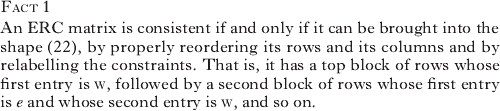
(53)
6.3 An invariant for calibrated re-ranking rules
The sum of the current RVs in (16b) is 155 (10+5+20+15+100+5). The updated RVs in (52) add up to 154·6. The fact that the sum of the updated RVs is smaller than that of the current RVs is not a coincidence, but rather a general property of calibrated re-ranking rules. Let me illustrate this, focusing on the calibrated re-ranking rule in (51). Suppose that the ERC triggering the current update has l undominated loser-preferrers and w winner-preferrers. The demotion component (51a) subtracts the demotion amount 1 from the RV of each of the l undominated loser-preferrers, so that the sum of the current RVs is decreased by l=1×l overall. The promotion component (51b) adds the promotion amount l/(w+1) to the RV of each of the w winner-preferrers, thus increasing the sum of the current RVs by (l/(w+1))×w overall. As the amount that is added to the sum of the current RVs (wl/(w+1)) is always smaller than the amount that is subtracted (l), the sum of the current RVs decreases at each update. The amount by which it decreases can be computed as in (54).
(54)
To trigger an update, the current ERC must have at least one undominated loser-preferrer, i.e. l must be at least 1. As the number of constraints is n and at least one of them is loser-preferring, there can be at most n−1 winner-preferrers, i.e. w can be at most n−1. Replacing l with 1 and w with n−1 in the right-hand side of (54), I conclude that at each update the sum of the current RVs decreases by at least 1/n. 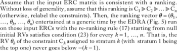
6.4 Calibration ensures efficient convergence
The proof of efficient convergence now follows straightforwardly. Consider a run of the EDRA on a consistent ERC matrix using the calibrated re-ranking rule in (51). Suppose for concreteness that the initial RVs are all null. As the input ERC matrix is consistent by hypothesis, the generalised Fact 2 ensures that the current RVs θ1, …, θn cannot become too small, as in (53). Because of the identity 0+1+2+…+(n −1)=n(n−1)/2, (53) entails that the sum of the current RVs never gets smaller than the constant −n(n−1)/2 (which only depends on the number n of constraints), as stated in (55).
(55)
By Fact 3, the sum of the current RVs decreases by at least 1/n with every update. After T updates, it thus has decreased by at least T/n. As we start from initial null RVs, the sum of the current RVs after T updates is thus smaller than or at most equal to −T/n, as in (56).
(56)
By combining together the two inequalities (55) and (56), we get the upper bound (57) on the number T of updates. In other words, as the sum of the current RVs decreases by at least 1/n with every update but cannot get smaller than −n(n−1)/2, then the algorithm cannot perform too many updates, i.e. no more than n 2(n−1)/2.
(57)
We have thus proved Theorem 2, which guarantees efficient convergence for the calibrated promotion/demotion re-ranking rule in (51). The reasoning just outlined easily extends to an arbitrary calibrated re-ranking rule, with the quality of the error-bound depending on how much the promotion amount is smaller than the calibration threshold l/w; see Appendix B of the online supplementary materials for details. The extension from null initial RVs to arbitrary ones is straightforward, as discussed in Appendix A of the online supplementary materials.

This section started from the intuition that the good convergent behaviour of demotion-only EDRAs should be retained or only slightly affected provided that the promotion component of the re-ranking rule does not overwhelm the demotion component. This requires a proper calibration of the promotion amount, as in the new calibrated re-ranking rule (51). Theorem 2 confirms that this initial intuition is correct. In fact, T&S's Theorem 1 ensures an error-bound for demotion-only that grows only quadratically with the number of constraints, while Theorem 2 provides an error-bound for the new calibrated promotion/demotion re-ranking rule in (51) that is only slightly worse, growing cubically rather than quadratically in the number of constraints.
6.5 Summary
Tesar & Smolensky's (Reference Tesar and Smolensky1998) original proof of convergence for demotion-only, reviewed in §3, was based on two crucial properties of the sum of the current RVs. The first property is that this sum can never become smaller than a certain constant that depends on the number of constraints, as stated in (58a). The second property is that, as long as we perform demotion only, the current RVs can only decrease over time, and in turn their sum can only decrease, as stated in (58b). Convergence immediately follows: as the sum of the current RVs keeps decreasing by (58b), but by (58a) cannot decrease too much, then learning must stop at a certain point.
(58) The sum of the current RVs
a. can never become smaller than a certain constant;
b. starts at zero and decreases a little with every update.
Property (58a) has nothing to do with the promotion issue. Rather, it follows from the fact that constraints cannot drop too much, as long as we only demote the constraints that really need to be demoted, namely the currently undominated ones. This property thus extends to any re-ranking rule that only demotes undominated loser-preferrers (generalised Fact 2). The case of property (58b) is more difficult. For instance, it does not hold for Boersma's GLA re-ranking rule in (40): if there are two winner-preferrers that are each promoted by 1 and one loser-preferrer that is demoted by 1, then the sum of the RVs increases by 1, instead of decreasing. Yet property (58b) is not altogether incompatible with constraint promotion. In fact, calibration of the promotion amount was designed in §6.1 in order to ensure that the sum of the current RVs decreases with each update, despite promotion (Fact 3). Convergence for calibrated promotion/demotion re-ranking rules follows again from the two properties in (58).
7 Calibration is a necessary condition for efficient convergence
§6 has shown that efficient convergence holds for re-ranking rules that perform both constraint demotion and promotion, as long as the promotion component of the update never overwhelms the demotion component. This requires the promotion amount to be calibrated: it must always be strictly smaller than the calibration threshold l/w, which is the ratio between the number l of currently undominated loser-preferrers and the number w of winner-preferrers. To complete the computational theory of re-ranking rules that perform both constraint demotion and promotion, I now want to investigate the limiting case where the promotion amount is set equal to the calibration threshold l/w, as described in §7.1. The proof of convergence for calibrated re-ranking rules developed in §6 does not extend to this limiting case, as explained in §7.2. A different line of analysis is thus needed, to be developed in §7.4. This analysis exploits a property of EDRAs that is interesting in its own right: they can never entertain a ranking (vector) that has made a mistake at some earlier time, as explained in §7.3. In other words, they explore the typology in an effective way: although EDRAs do not keep track of previously seen data and thus of previously made errors, they implicitly manage to avoid repeating the same error twice. This alternative proof of convergence does not provide a bound on the number of errors made before converging. §7.5 takes on the issue of the number of errors, showing how to construct cases where even the best-case number of errors grows exponentially in the number of constraints. In conclusion, efficiency breaks down at the calibration threshold l/w, and proper calibration is thus a necessary condition for efficient convergence.
7.1 Smallest non-calibrated promotion
In this section, I study the re-ranking rule in (59). Its crucial property is that the promotion amount is set equal to the calibration threshold l/w, namely the ratio between the number l of undominated loser-preferrers and the number w of winner-preferrers. In other words, this is the update rule with the smallest possible promotion amount among those which are not calibrated and thus do not fall under the theory developed in §6.
- (59)
a. Decrease the RV of each of the l undominated loser-preferrers by 1.
b. Increase the RV of each of the w winner-preferrers by l/w.
For instance, if the current ERC and ranking vector are again as in (16), then the updated ranking vector is (60). Of the two loser-preferrers C4 and C6, only the former is currently undominated. Its RV is thus decreased by 1. The RV of the two winner-preferrers C1 and C2 is increased by 1/2, i.e. the number of undominated loser-preferrers (l=1) divided by the number of winner-preferrers (w=2).
(60)
7.2 An invariant for smallest non-calibrated promotion
The sum of the current RVs in (16b) is 155. The updated RVs in (60) add up to the same number. The fact that the sum of the current RVs remains constant is not a coincidence. In fact, the promotion component (59b) of the re-ranking rule adds the promotion amount l/w to the RV of each of the w winner-preferrers, so that the sum of the current RVs is increased by (l/w)×w=l overall. Furthermore, the demotion component (59a) subtracts the demotion amount 1 from the RV of each of the l loser-preferrers, so that the sum of the current RVs is decreased by 1×l=l overall. As the same quantity is added to and subtracted from the sum of the current RVs, the promotion and demotion components of the re-ranking rule balance each other, and the sum of the current RVs remains constant over time.

Unfortunately, Fact 4 entails that the strategy used in §6 to prove convergence for the case of calibrated promotion amounts does not extend to the case of the smallest non-calibrated promotion amount (59). T&S's lower bound on the sum of the current RVs holds for any re-ranking rule (as long as only undominated loser-preferrers are demoted), as stated in generalised Fact 2. If the sum of the current RVs decreases with each update (as in the case of demotion-only or calibrated promotion), then T&S's lower bound on the sum of the RVs straightforwardly translates into a bound on the number of possible updates. But if the sum of the current RVs does not decrease with each update, but rather stays constant, T&S's lower bound does not straightforwardly have anything to say about the number of updates. A more indirect reasoning is needed, illustrated in §7.4. This alternative analysis rests on another property of EDRAs discussed in §7.3, namely that they cannot loop.
7.3 EDRAs cannot loop
The sequence of ranking vectors entertained by a demotion-only EDRA cannot contain a sub-sequence such as (61), whereby the same ranking vector θ is entertained at two different times but with some other ranking vector θ′≠θ entertained at some time in between. The reason is straightforward. When moving from the ranking vector θ=(θ1, …, θn) to a different ranking vector θ′=(θ′1, …, θ′n), at least one RV must have decreased from θk to some smaller value θ′k. In order for the algorithm to go back from θ′ to θ, that RV would need to increase from θ′k to its original value θk. This is impossible with a demotion-only re-ranking rule, as RVs can only decrease but not increase over time.
(61)
Thus demotion-only EDRAs cannot loop: once a ranking vector is deemed unsuitable, and is therefore updated, the algorithm can never consider it again in the same learning path. In other words, demotion-only EDRAs explore the search space in an effective way, as they avoid entertaining the same incorrect hypothesis twice.
This special property does not carry over from demotion-only to promotion/demotion EDRAs. A trivial counterexample is provided in (62). Start from a null initial ranking vector. Update in response to the ERC 1, according to the promotion/demotion re-ranking rule in (59). Then update again in response to the ERC 2. The algorithm has looped back to the initial null ranking vector.
(62)
The details of the re-ranking rule are irrelevant here. The point is that, as soon as we perform some constraint promotion, RVs can oscillate up and down, and in particular can return to values entertained earlier.
Yet the input ERC matrix (62a) used to get the EDRA to loop is inconsistent. What if we restrict ourselves to consistent ERC matrices? Fact 5 ensures that EDRAs cannot loop in this case, even if the re-ranking rule performs constraint promotion as well as demotion. Again, the details of the re-ranking rule do not matter, and the statement holds for any re-ranking rule of the form (46).Footnote 15
 In the demotion-only case, the impossibility of loops follows trivially from the monotonicity of the ranking dynamics, and is thus independent of the properties of the input ERC matrix. In the promotion/demotion case, however, the impossibility of loops follows from a property of the input ERC matrix, namely its consistency. Understanding why promotion/demotion EDRAs cannot loop thus brings out an interesting and non-trivial property of the notion of OT-consistency. In particular, non-looping follows from a connection between OT-consistency and the geometric property of conic independence. The details of this reasoning can be found in Appendix C of the online supplementary materials.
7.4 Convergence
We are now able to prove convergence for the re-ranking rule in (59), with the smallest non-calibrated promotion amount. Recall first generalised Fact 2 from §6.2, which guarantees that T&S's lower bound on the current RVs holds for any re-ranking rule that demotes only the loser-preferrers which need to be demoted, i.e. the undominated ones. Thus, the current RVs in any run of the EDRA with the re-ranking rule (59) cannot become arbitrarily small, provided the input ERC matrix is consistent.
Can the current RVs get arbitrarily large? As seen is §5.2, this is precisely what happens when Boersma's GLA (40) is run on Pater's counterexample in (42): the RVs increase indefinitely. But this cannot happen in the case of (59). In fact, the RVs all start out null. As, by Fact 4, their sum must remain constant over time, the current RVs must always add up to zero. As they cannot become too small and must add up to zero, the current RVs cannot become too large either.
As the current RVs cannot become too large or too small, the current ranking vector must live in a bounded region. Each time a RV is updated, it is increased by 1, or by at least 1/n. This means in turn that the RVs entertained by the EDRA live on a grid of points, separated by at least 1/n from each other. As the search space of the algorithm consists of a bounded grid, it contains only a finite number of ranking vectors. Since the algorithm cannot loop by Fact 5, finiteness of the search space entails finite time convergence. We have thus proved the following convergence theorem.Footnote 16 For a very different proof, see Magri (to appear b).
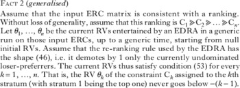
7.5 Number of errors
T&S's convergence Theorem 1 for demotion-only EDRAs provides a (tight) bound on the worst-case number of errors. Theorem 2 extends T&S's analysis to calibrated promotion/demotion EDRAs, with a comparable bound on the worst-case number of errors. Unfortunately, that analysis does not extend to the case of the non-calibrated re-ranking rule (59) considered here. An alternative analysis thus had to be developed in order to prove the convergence Theorem 3. This alternative analysis does not provide a bound on the worst-case number of errors. This final section examines this issue, showing that the worst-case number of errors in the case of the non-calibrated re-ranking rule (59) grows exponentially with the number of constraints, so that efficiency is lost.
Following Riggle (Reference Riggle2009), let the diagonal matrix for n constraints be the ERC matrix with n columns and n−1 rows, whose kth row has all entries equal to e, except for the kth entry, which is a w, and the following entry, which is an l. To illustrate, I give in (63) the diagonal ERC matrices for n=4, 5, 6 constraints.
(63)
For diagonal matrices, a different line of analysis developed in Magri (to appear b) guarantees that the worst-case number of errors made by the EDRA with the non-calibrated re-ranking rule (59) is feasible (smaller than n(n 2−1)/6, where n is the number of constraints).
Pater (Reference Pater2008) considers ERC matrices obtained from the diagonal one by adding a w to the right of every l. More precisely, let Pater's matrix for n constraints be the ERC matrix with n columns and n−1 rows obtained from the diagonal matrix by ‘adding’ a w at the right of every l (except in the last row). The case with n=5 was considered in (42). To illustrate, I give in (64) Pater's matrices for n=4, 5, 6 constraints.
(64)
The extra w's added at the right of the diagonal in Pater's matrices do not contribute anything to consistency, in the sense that they do not enlarge the set of consistent rankings. They only serve the purpose of confounding re-ranking rules that perform constraint promotion and are thus sensitive to these w's. Indeed, Pater's extra layer of w's is able to fool the GLA, as observed in §5.3. But it is not able to fool the non-calibrated re-ranking rule in (59): the analysis developed in Magri (to appear b) guarantees again a feasible worst-case number of errors (smaller than n 5, where n is the number of constraints).
Let us try to further aggravate the learning challenge by adding yet another layer of useless w's. Let the Aggravated Pater's matrix for n constraints be the ERC matrix with n columns and n−1 rows obtained from the diagonal matrix by ‘adding’ two w's (rather than just one) at the right of every l (except for the penultimate row, where only one w is added, and the last row, where no w's are added). In (65) I give the aggravated Pater's matrices for n=4, 5, 6 constraints.
(65)
Theorem 3 guarantees that the EDRA with the non-calibrated re-ranking rule in (59) converges on aggravated Pater's matrices. Yet it turns out that convergence is not efficient: even in the best, shortest run, the algorithm makes far too many errors before it finally converges on a consistent ranking vector. In Appendix D of the online supplementary materials, I show how to compute the best-case number of mistakes made by the EDRA with rule (59) on aggravated Pater's matrices. The computation is analogous to the explanation provided in §5.3 for Pater's counterexample to the GLA's convergence. The best-case number of errors is provided in Table Ia for various choices of the number n of constraints. For instance, the EDRA will always perform no fewer than 107,920 updates before converging to a ranking vector consistent with the aggravated Pater's matrix corresponding to n=15 constraints.
(a) best-case number of errors performed by the EDRA with the smallest non-calibrated promotion amount (59), run on the aggravated Pater's matrix for n constraints; (b) value of 2n for corresponding values of n.

In Table Ib, I report the values of 2n for the corresponding values of n. The table thus shows that the best-case number of mistakes made by the EDRA with the re-ranking rule (59) on aggravated Pater's matrices grows exponentially with the number of constraints. In other words, the number of mistakes performed before reaching convergence grows so quickly with n that it is unfeasible even for a small number of constraints.
7.6 Summary
This section has studied re-ranking rule (59), which increases the promotion amount to the calibration threshold l/w, namely the ratio between the number l of undominated loser-preferrers and the number w of winner-preferrers. It has shown that convergence is retained in this case, but efficiency is lost: an exponential number of errors might be required before reaching convergence. This result is somewhat surprising. One might expect that, in order to bring down the number of errors from exponential to something feasible, the promotion amount would need to be exponentially reduced, so as to become practically useless from the modelling perspective of §4. This intuitively plausible conjecture turns out to be false. In fact, as seen in §6, it is sufficient to decrease the promotion amount just slightly, for example from l/w to l/(w+1), in order to obtain efficient convergence. This shows the importance of a thorough computational understanding of the algorithm when setting the implementation parameters of the model.
8 Conclusion
§2 reviewed an important learning scheme in the computational OT literature, EDRAs. The crucial property of EDRAs is that they are trained on a stream of data and predict a sequence of ranking vectors. The switch from the current ranking vector to the updated one is prompted by an error on the current piece of data. The crucial implementation detail for EDRAs is the re-ranking rule used by the algorithm to switch from the current to the updated ranking vector. In this paper, I have focused on re-ranking rules of the form (46). Only loser-preferrers that need to be demoted are indeed demoted, i.e. only the currently undominated ones. They are demoted by a small fixed demotion amount, say 1 for concreteness. All winner-preferrers are promoted by a promotion amount p, which can be null or positive.
A computationally sound EDRA should eventually stop making errors on the training sequence of data, and thus settle on a ranking vector consistent with the input data (convergence). Furthermore, the number of errors made before reaching convergence should not grow exponentially with the number of constraints (efficiency). Within (46), then, the crucial issue is how to choose the promotion amount p to ensure efficient convergence.
Building on previous work (in particular Boersma Reference Boersma1997, Reference Boersma1998, Tesar & Smolensky Reference Tesar and Smolensky1998 and Pater Reference Pater2008), this paper has developed a complete answer to this question, summarised in (66). The pivot of the theory is the calibration threshold, namely the ratio l/w between the number l of undominated loser-preferrers that are demoted and the number w of winner-preferrers that are promoted.
(66)
As reviewed in §3, T&S showed that efficient convergence holds for demotion-only re-ranking rules, i.e. rules of the form (46) with a null promotion amount (i.e. p=0). Building on their analysis, §6 showed that efficient convergence extends (with comparable error-bounds) from demotion-only re-ranking rules to calibrated promotion/demotion re-ranking rules, i.e. rules of the form (46) with a promotion amount strictly smaller than the calibration threshold (i.e. p<l/w). This result cannot be extended any further. In fact, §7 looked at re-ranking rules of the form (46) with a promotion amount that coincides with the calibration threshold (i.e. p=l/w), and showed that, although convergence holds, efficiency breaks down, as the number of errors can grow exponentially in the number of constraints. The calibration threshold is thus the tipping point for the theory of EDRAs' convergence. Above that threshold, convergence is lost as well. Indeed, in §5 I discussed in detail Pater's (Reference Pater2008) counterexample, which shows that convergence also breaks down once we pass the calibration threshold, namely for re-ranking rules of the form (46) with a promotion amount that exceeds the calibration threshold (p>l/w), such as Boersma's re-ranking rule with p=1.
The focus of the paper has been mainly computational, looking at the crucial learnability requirement of EDRAs' efficient convergence. However, §4 provided an initial glimpse into the modelling implications of these computational results. I have looked at an application of EDRAs that has figured prominently in the literature, namely modelling the early acquisition of phonotactics. It is common in this literature to assume that the child posits underlying forms faithful to the adult winner forms. As Pater & Barlow (Reference Pater and Barlow2003: 490) write, ‘the [underlying form] in … child phonology [is] taken to correspond to the child's stored lexical representation’ under the assumption that it ‘is likely [that] children do perceive and store [forms] accurately’. This assumption makes good sense computationally, as it never leads to inconsistent ERCs (under mild assumptions on the constraint set), as shown by Tesar (Reference Tesar2008). In this paper, I have pointed out the modelling implications of this assumption that EDRAs be trained on faithful mappings. This assumption predicts that faithfulness constraints are never loser-preferrers. Hence they would never be re-ranked by a demotion-only re-ranking rule. I have argued that this cannot be right from the perspective of the restrictiveness of the final grammar, namely how well it rules out illicit forms. Also, it cannot be right from the perspective of the matching between predicted learning sequences and acquisition paths. The current literature thus displays a gap between what the OT acquisition literature needs (namely sound EDRAs that perform both constraint promotion and demotion) and what the OT computational literature has been able to deliver (namely EDRAs that are sound but don't perform constraint promotion, such as EDCD, or EDRAs that perform constraint promotion but are not sound, such as the GLA). This paper has filled this gap: it develops sound EDRAs that also perform constraint promotion, through a proper calibration of the promotion amount. These results thus contribute to a general line of research that tries to establish EDRAs as proper models of the child acquisition of phonotactics, both from a computational and a modelling perspective.