1. Introduction
Columnar vortices impacting a surface can be separated into three classes of interactions: (i) parallel, (ii) normal, or (iii) streamwise (perpendicular) vortex–body encounters, with an excellent and extensive review of each of these interactions provided by Rockwell (Reference Rockwell1998). While the unsteady physics of the first two vortex representations have been well documented, considerably less attention has been paid to streamwise-oriented vortex–body interactions; in particular, to the unsteady, three-dimensional nature of the vortex and how it relates to the induced loading on a finite wing as would be encountered, for example, in turbomachinery blade-row interactions (Zanotti et al. Reference Zanotti, Ermacora, Campanardi and Gibertini2014), fin buffeting (Gursul & Xie Reference Gursul and Xie2001; Lambert & Gursul Reference Lambert and Gursul2004), or formation flight (Hummel Reference Hummel1983, Reference Hummel1995). Even less understood are the implications of a wandering vortex impinging upon a wing that not only dynamically shifts from the upstream influence of the wing, but also from wing deformations, atmospheric turbulence, or crow-instability effects, to name a few.
Either a single vortex or systems of streamwise-oriented vortices are known to exhibit rich dynamics. Long wavelength (Crow Reference Crow1970), short wavelength (elliptical) and spiral breakdown (Gordnier & Visbal Reference Gordnier and Visbal1999) constitute examples of potential outcomes that may affect the evolution of a streamwise-oriented vortex and its interaction with aerodynamic surfaces encountered in its path. Furthermore, axial vortices may also exhibit spiral substructures generated during their roll-up process (Visbal & Gordnier Reference Visbal and Gordnier2003; Richez et al. Reference Richez, Le Pape, Costes and Gavériaux2012). These instabilities and unsteady features can result in additional sources of buffeting while impinging upon a finite wing. To further compound the problem, either deliberate or unanticipated motions of the incident vortex can provide another degree of uncertainty in the predicted flow structure, even experimentally. Heyes, Jones & Smith (Reference Heyes, Jones and Smith2004), for example, discuss the difficulties in extracting reliable measurements from wandering vortices and demonstrate how vortex wandering effects must be corrected to prevent false conclusions from being drawn about the vortex structure, i.e. breakdown. These difficult-to-predict unsteady phenomena engendered by the vortex/surface interaction will impact the unsteady loading or buffeting experienced by the wing. Another unresolved critical aspect of the problem is the modification of the incident vortex and its instability modes generated by the process of impingement upon the wing. This feedback will most likely be limited to a region of upstream influence in front of the wing. Nonetheless, coupling of vortex instabilities with the unsteady separation is, in general, not well understood and could give rise to a resonant behaviour with significant impact on the vortex/surface interaction.
Streamwise-oriented vortex/wing interactions in the context of formation flight, which has long been understood to provide significant benefits in aerodynamic performance, have been analysed in a series of papers by Hummel (Reference Hummel1983, Reference Hummel1995) and Beukenberg & Hummel (Reference Beukenberg and Hummel1990) using classic aerodynamic theory, wherein citations to earlier seminal work can also be found. With proper positioning, trailing aircraft can capture the upwash from the tip vortex left in the wake of a lead aircraft. The result is a forward-tilted lift vector that provides increased lift and a reduction in induced drag and can lead to significant energy savings (Lissaman & Shollenberger Reference Lissaman and Shollenberger1970). Recently, Ning, Flanzer & Kroo (Reference Ning, Flanzer and Kroo2010) performed an investigation of several factors affecting the benefits and feasibility of extended formation flight for three aircraft in canonical echelon and V-type arrangements. These factors included wake roll-up, vortex core size, vortex decay and gust effects. Kless et al. (Reference Kless, Aftosmis, Ning and Nemec2013) provided a computational inviscid flow analysis of several aspects of extended formation flight, with consideration of optimal incident vortex location, roll trim effects and transonic flow effects. Vortex meandering induced from wind-tunnel unsteadiness, atmospheric turbulence, crow instability, or upstream feedback from the surface (Jacquin, Fabre & Geffroy Reference Jacquin, Fabre and Geffroy2001), can also pose a problem for reliable wake capturing in this context, wherein significant deviation of the impacting vortex core can lead to unintended separation or unsteady loading. In the tandem wing experiments of Inasawa, Mori & Asai (Reference Inasawa, Mori and Asai2012), maximum advantage of lift-to-drag ratio was also observed when the wings were overlapped in the spanwise direction. Additionally, a comprehensive multi-fidelity computational analysis of formation flight has been provided by Slotnick et al. (Reference Slotnick, Clark, Friedman, Yadlin, Yeh, Carr, Czech and Bieniawski2014). Most notably, trimmed aerodynamic benefit maps were developed to uncover the best formation positioning for optimal performance, and the Reynolds-averaged Navier–Stokes (RANS) computational method coupled with a wake evolution solver was found to yield comparable time-averaged quantities to flight test data. Despite advances in the basic prediction and demonstration of the benefits of formation flight, significant challenges still exist in the understanding and implications of the unsteady loading and flow structure incurred from formation flight before this technology becomes a viable and safe operational capability.
The recent high-fidelity numerical studies of Garmann & Visbal (Reference Garmann and Visbal2014) and Barnes, Visbal & Gordnier (Reference Barnes, Visbal and Gordnier2015) (the precursor to the current work) have brought insight into the unsteady interactions of a streamwise-oriented vortex impinging upon a finite wing. In the former, two aspect-ratio-six flat plate wings, arranged in tandem, were simulated at a Reynolds number of 30 000 as a generic problem of formation-flight-like conditions. Several spanwise positions and incidence angles of the lead wing were varied for both rigid and flexible follower wings in an effort to engender the most significant aeroelastic response. The resulting flow structure with outboard positioning yielded vortex dipole-like pairing between the incident and tip vortices, while more inboard locations presented a time-mean bifurcation of the incident vortex. It was concluded from the unsteady loading that lead-wing wandering may be a more dominant driver of structural response. Additionally, wing compliance led to a substantial repositioning and stabilizing effect of the incident vortex.
In this work, a high-fidelity, implicit large-eddy simulation (ILES) approach is utilized to characterize the unsteady modes of interaction resulting from a streamwise-oriented vortex impinging upon a finite plate for various spanwise positions. An analytically defined vortex is superimposed into a free stream and convected towards a flat plate wing as a controlled canonical problem of perpendicular vortex/surface interactions. The simplified vortex/wing configuration allows many vortex positions, strengths and sizes to be readily examined without the need for detailed simulation of a lead wing, making it an ideal problem for careful study of the impingement problem, which is poorly understood. With so many interrelated parameters (Reynolds number, surface curvature, vortex stability, etc.) that may lead to different behaviours, it is necessary to study a problem that controls these parameters to some extent so as to uncover the flow’s dependence on each. The focus here is limited to a simple flat plate configuration at a low Reynolds number to facilitate a strong vortex interaction with a separated, unsteady flow.
2. Numerical procedure
All simulations are performed with the extensively validated high-order, compressible Navier–Stokes flow solver, FDL3DI (Gaitonde & Visbal Reference Gaitonde and Visbal1998; Visbal & Gaitonde Reference Visbal and Gaitonde1999). In this code, the unfiltered, strong conservation-law form of the governing equations is used without change in laminar, transitional or fully turbulent regions of the flow for the ILES procedure. Unlike the standard LES approach, no additional subgrid-scale (SGS) model or heat flux terms are appended. Instead, a high-order, low-pass filter operator, which will be discussed later, is applied to the conserved variables during the solution of the standard Navier–Stokes equations. This highly discriminating filter selectively damps only the high-frequency components of the solution that are under-resolved by the mesh (Visbal & Rizzetta Reference Visbal and Rizzetta2002). The filtering regularization procedure provides an attractive alternative to the use of standard SGS models, and has been found to yield suitable results for turbulent and transitional flows on LES level grids (Garmann, Visbal & Orkwis Reference Garmann, Visbal and Orkwis2013). A reinterpretation of this ILES approach in the context of an Approximate Deconvolution Model (Stolz & Adams Reference Stolz and Adams1999) has been provided by Matthew et al. (Reference Matthew, Lechner, Foysi, Sesterhenn and Friedrich2003). For low Reynolds numbers and/or high spatial resolutions, the ILES approach is effectively direct numerical simulation (DNS).
The governing equations are solved in a non-dimensional form, where all flow variables are normalized by their respective free stream counterparts, except for pressure, which is scaled by twice the dynamic pressure,
 ${\it\rho}_{\infty }U_{\infty }^{2}$
. The reference length is taken as the wing chord,
 $c$
. A perfect gas is also assumed,
 $p={\it\rho}T/{\it\gamma}M_{\infty }^{2}$
, along with Sutherland’s viscosity law and Stokes’ hypothesis for the bulk viscosity coefficient (
 ${\it\lambda}=-2/3{\it\mu}$
). The Prandtl number is prescribed as
 $\mathit{Pr}=0.72$
for air.
All spatial derivatives are obtained numerically using high-order compact-differencing schemes (Lele Reference Lele1992) along a coordinate line in computational space, which requires solution of a tridiagonal system. At boundary points, higher-order, one-sided formulae are utilized that retain the tridiagonal form of the scheme (Gaitonde & Visbal Reference Gaitonde and Visbal1998; Visbal & Gaitonde Reference Visbal and Gaitonde1999). For all the computations presented in this work, the interior compact scheme is sixth-order accurate, while the boundary point and first off-boundary point use fourth- and fifth-order compact schemes, respectively. The derivatives of the inviscid fluxes are obtained by forming the fluxes at the nodes and differentiating each component with the compact-differencing scheme. Viscous terms are obtained by first computing the derivatives of the primitive variables and then constructing the components of the viscous fluxes at each node and differentiating by a second application of the same scheme.
In order to eliminate spurious components of the solution, a high-order, low-pass spatial filtering operator (Gaitonde & Visbal Reference Gaitonde and Visbal1999; Visbal & Gaitonde Reference Visbal and Gaitonde1999) is applied to the conserved variables along each transformed coordinate direction one time after each time step or sub-iteration. The filtering technique is based on templates proposed by Alpert (Reference Alpert1981) and Lele (Reference Lele1992) and provides a
 $2N$
th-order formula on a
 $2N+1$
point stencil. The coefficients, along with representative filter transfer functions, can be found in the works of Gaitonde & Visbal (Reference Gaitonde and Visbal1998, Reference Gaitonde and Visbal1999). A free parameter,
 ${\it\alpha}_{f}$
, is left to provide limited control of the cutoff frequency of the low-pass filter operator. Typical values are in the range:
 $0.3\leqslant {\it\alpha}_{f}\leqslant 0.49$
, where higher values lead to less dissipation. For the near-boundary points, the filtering strategies described by Gaitonde & Visbal (Reference Gaitonde and Visbal1999) and Visbal & Gaitonde (Reference Visbal and Gaitonde1999) are used. For transitional and turbulent flows, the high-fidelity spatial algorithmic components provide an effective ILES approach in lieu of traditional SGS models, as demonstrated by Visbal & Rizzetta (Reference Visbal and Rizzetta2002) and Visbal, Morgan & Rizzetta (Reference Visbal, Morgan and Rizzetta2003), and more recently by Garmann et al. (Reference Garmann, Visbal and Orkwis2013). All computations presented in this work utilized an eighth-order accurate interior filter to preserve the sixth-order accuracy of the solution, along with a coefficient of
 ${\it\alpha}_{f}=0.4$
for targeted dissipation of only the highest wavenumbers.
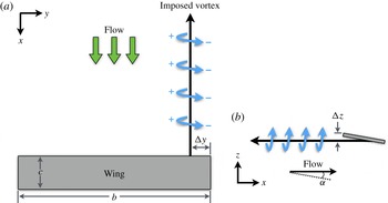
Configuration of a streamwise-oriented vortex impinging on a wing. (a) Top view; (b) side view.

Time marching of the governing equations is achieved through the implicit approximately factored integration method of Beam & Warming (Reference Beam and Warming1978), which is supplemented with the use of Newton-like sub-iterations to achieve second-order accuracy (Visbal & Rizzetta Reference Visbal and Rizzetta2002; Visbal et al. Reference Visbal, Morgan and Rizzetta2003). In delta form, spatially second-order finite differences are used within the implicit operator, while high-order compact differencing is employed within the residual. The block-tridiagonal form of the equations are further simplified through the diagonalization of Pulliam & Chaussee (Reference Pulliam and Chaussee1981), and fourth-order, nonlinear dissipation terms (Jameson, Schmidt & Turkel Reference Jameson, Schmidt and Turkel1981; Pulliam Reference Pulliam1986) are also appended to the implicit operator to augment stability. Iteration reduces errors associated with factorization, linearization, diagonalization, and explicit application of boundary conditions (Rizzetta, Visbal & Morgan Reference Rizzetta, Visbal and Morgan2008), while also driving the lower-order error of the implicit operator to zero and leaving only the high-order spatial error of the residual.
3. Details of the computations
3.1. Geometry and vortex model
An analytically defined vortex is superimposed on a free stream and convected towards a wing, as shown in figure 1. The rectangular, flat plate wing has an aspect ratio of six (
 $\mathit{AR}=b/c=6$
) and a thickness of
 $t=0.03c$
and is oriented at an angle of attack of
 ${\it\alpha}=4^{\circ }$
relative to the free stream, operating at a Reynolds number of
 $\mathit{Re}=20\,000$
. With so little known about the unsteady modes of perpendicular vortex/surface interactions and with so many interrelated parameters (Reynolds number, surface curvature, vortex stability, etc.) that may lead to different behaviours, it is necessary to study a problem that controls these parameters to some extent so as to uncover the flow’s dependence on each. The selection of this particular geometry was based on several factors. Firstly, Reynolds number was limited both by available computational resources and tractability for LES, so a NACA wing, for example, at the selected conditions would have resulted in a laminar and attached flow; however, it was desirable to facilitate an interaction with a separated, unsteady flow over the wing, which is guaranteed by a flat plate at the chosen conditions. Secondly, the flat plate allows characterization of the unsteady flow regimes in lieu of curvature effects. Cambering of the plate to alleviate the adverse pressure gradient over the wing is a natural step for a follow-on study to build upon the results contained here by adding complexity in stages so as to trace the source of certain flow features. Finally, the flat plate is a generic surface that is easily modelled and manufactured, making it suitable for complementary computational and experimental studies that cover a range of applications. A more streamlined, airfoil cross-section is planned for future investigations at higher Reynolds numbers and will certainly be of interest.
In order to model the incident vortex, a Batchelor or
 $q$
-vortex vortex (Batchelor Reference Batchelor1964) is superimposed into the incoming flow upstream of the wing. This vortex is described analytically as
 $$\begin{eqnarray}\displaystyle & u_{r}(r)=0 & \displaystyle\end{eqnarray}$$
 $$\begin{eqnarray}\displaystyle & \displaystyle u_{{\it\theta}}(r)=\frac{{\it\Gamma}_{0}}{2{\rm\pi}r}(1-\text{e}^{-(r/r_{0})^{2}}) & \displaystyle\end{eqnarray}$$
 $$\begin{eqnarray}\displaystyle & u_{x}(r)=1-{\rm\Delta}u\text{e}^{-(r/r_{0})^{2}} & \displaystyle\end{eqnarray}$$
 $u_{r}$
,
 $u_{{\it\theta}}$
and
 $u_{x}$
correspond to the radial, circumferential and axial velocities, respectively,
 ${\it\Gamma}_{0}$
is the vortex circulation,
 $r_{0}$
is a measure of the vortex radius, and
 ${\rm\Delta}u$
is the axial velocity deficit in the vortex core. Rather than circulation, the swirl parameter,
 $q$
, is used to specify the strength of the vortex. This parameter is defined as
 $$\begin{eqnarray}q=\frac{{\it\Gamma}_{0}}{2{\rm\pi}r_{0}{\rm\Delta}u}\approx 1.567\frac{V_{0}}{{\rm\Delta}u}\end{eqnarray}$$
where
 $V_{0}$
is the maximum circumferential velocity. This shows that
 $q$
is a measure of the relative tangential and axial velocity intensities (Jacquin & Pantano Reference Jacquin and Pantano2002). The circumferential velocity recast in terms of
 $q$
becomes
 $$\begin{eqnarray}u_{{\it\theta}}(r)=\frac{q{\rm\Delta}u}{r/r_{0}}(1-\text{e}^{-(r/r_{0})^{2}}).\end{eqnarray}$$
A stability criterion for the
 $q$
-vortex was established by Leibovich & Stewartson (Reference Leibovich and Stewartson1983) to prevent amplification of small-wave perturbations at any
 $r$
. This restriction is given as
 $$\begin{eqnarray}{\it\sigma}^{2}(r)=\frac{2u_{{\it\theta}}(ru_{{\it\theta}}^{\prime }-u_{{\it\theta}})(u_{{\it\theta}}^{2}/r^{2}-u_{{\it\theta}}^{\prime 2}-u_{x}^{\prime 2})}{(ru_{{\it\theta}}^{\prime }-u_{{\it\theta}})^{2}+(ru_{x}^{\prime })^{2}}<0.\end{eqnarray}$$
Substitution of (3.3) and (3.5) into the stability criterion leads to a lower bound prediction on the swirl parameter of
 $q\geqslant \sqrt{2}$
to maintain stability of the vortex.
For the cases presented here, the swirl parameter is selected as
 $q=2.0$
to prevent the vortex from becoming susceptible to breakdown before interacting with the wing. To achieve a maximum circumferential velocity of
 $V_{0}=0.5U_{\infty }$
, the axial velocity deficit is chosen as
 ${\rm\Delta}u=0.4U_{\infty }$
. The vortex core radius is set as
 $r_{0}=0.1c$
, and the Reynolds number based on wing chord and free stream velocity is selected as
 $\mathit{Re}=20\,000$
to ensure tractability for LES. The reference Mach number is selected as
 $M_{\infty }=0.1$
in order to largely avoid effects of compressibility. Each of these parameters has been selected based on vortex profiles documented within the literature by the Euler computations of Kless et al. (Reference Kless, Aftosmis, Ning and Nemec2013) and the experiments of Inasawa et al. (Reference Inasawa, Mori and Asai2012) in which a lead wing was actually tested and the wake was analysed. The estimated values for the maximum circumferential velocity and its radial location are listed in table 1 along with details of the lead wing geometry and orientation. The maximum velocity radial location,
 $r_{u_{max}}$
, is related to the core radius of the
 $q$
-vortex by
 $r_{u_{max}}\approx 1.121r_{0}$
, leading to the choice of
 $r_{0}/c=0.1$
for the current study, which falls within the range of values appearing in the reported literature.
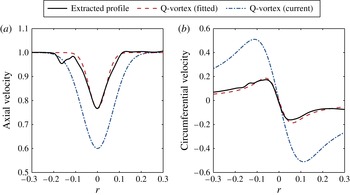
Matching of a
 $q$
-vortex to the tip vortex of a flat plate wing. Extracted profile is taken
 $1.5c$
downstream of a flat plate wing in a free stream oriented at
 ${\it\alpha}=4^{\circ }$
. A fitted
 $q$
-vortex is shown along with the vortex used in this study with twice the swirl strength and core radius.

Vortex profiles from the literature.

Although the purpose of this study is to examine the taxonomy of a generic surface/plate interaction, it should be noted that the chosen parameters yield a vortex that mimics the nature of the trailing vortex generated by the flat plate wing at an angle of attack, only with approximately twice the swirl strength and core radius, as indicated in figure 2. Here, the tip vortex profile was extracted
 $1.5c$
behind the flat plate wing oriented at
 ${\it\alpha}=4^{\circ }$
in a free stream, and values for a
 $q$
-vortex are found to match quite closely to the physically generated tip vortex, which is characterized by an axial velocity deficit. However, the matched swirl number is below the stable limit of the
 $q$
-vortex, which could lead to breakdown of the incident vortex possibly before reaching the wing. For this reason, the matched swirl parameter and core radius were doubled to allow the incident vortex used in this study to operate simply as a scaled version of the physical vortex that could be generated by a larger leader wing in heterogeneous formations, for example. This scaled vortex is also plotted for comparison. The incoming vortex is initiated at the inflow boundary as laminar, therefore any turbulent fluctuations that develop result solely from the vortex/wing interaction, which could not have otherwise been discerned if the vortex were initially turbulent or prescribed with a swirl parameter below the stability threshold. Despite the differences in strength and size, similar interactions were observed between the initial studies of Garmann & Visbal (Reference Garmann and Visbal2014) of the analytically defined vortex and that of Barnes et al. (Reference Barnes, Visbal and Gordnier2015), where the tip vortex was generated by a lead flat plate wing, indicating that the simplified model can provide suitable results while dramatically reducing computational cost by eliminating the need to model a leader wing.
Additionally, preliminary computations, which are not presented here, showed that the vortex deflects upwards as it approaches the wing and could convect completely over the upper side when positioned at or above the leading edge in the vertical direction due to the accelerating flow over the lifting body. To prevent this and facilitate a more dynamic interaction of a head-on collision for this study, the incident vortex is, instead, positioned under the leading edge such that its axis intersects with the mid-chord of the wing (
 $z=0.035$
) in the vertical direction. Several spanwise positions of the incoming vortex are examined, corresponding to
 ${\rm\Delta}y=-0.25$
, 0, 0.25, 0.50 and 1.00. The first position is outboard of the wingtip, the second is tip-aligned, and the others are all inboard of the tip.
3.2. Computational mesh and boundary conditions
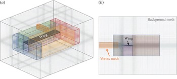
A nested mesh system that utilizes Chimera overset (Steger, Dougherty & Benek Reference Steger, Dougherty, Benek, Ghia and Ghia1983) with high-order interpolation (Sherer & Scott Reference Sherer and Scott2005) has been created to discretize the domain around the wing. The configuration consists of six near-body stretched Cartesian meshes protruding normal to the rectangular wing with increased stretching away from the surface. Once a nominal spacing has been achieved, the near-body grids cease and a coarser background mesh continues to the far-field boundaries, located 30–50 chords from the wing. A separate, higher-resolution mesh is overset into the background mesh to maintain the integrity of the streamwise-oriented vortex as it convects towards the wing from the inflow boundary. A depiction of the near-field, nested mesh system is presented in figure 3. The far-field boundaries actually extend much farther away from the wing, but only the near-body domain is shown for clarity. Additionally, the wing is oriented at an angle of
 ${\it\alpha}=4^{\circ }$
and the mesh is analytically deformed near the surface using a exponential decay weighting function to maintain normal gridlines at the boundary while keeping the mid-field overlap regions undisturbed away from the wing. This allows multiple wing orientations to be readily available by merely deforming the mesh rather than completely regenerating the discretized domain; although, only one orientation is considered in this study, i.e.
 ${\it\alpha}=4^{\circ }$
.
Depiction of the near-field nested mesh configuration. (a) Full view; (b) side view. Note that the far-field mesh actually extends 30–50 chords from the wing, but only the near field is shown for clarity.

The inflow boundary is positioned 10 chords ahead of the wing, and the analytically defined vortex is imposed there. All other far-field boundaries are prescribed as outflow conditions, which in conjunction with the increased grid-stretching and high-order filtering, provides a buffer-like treatment that prevents reflections from corrupting the interior of the domain. The wing surface is set as a no-slip, adiabatic wall enforced through a fourth-order-accurate, zero-normal pressure gradient.
3.3. Effects of spatial resolution
In order to examine the spatial resolution required for the current problem, three geometrically similar meshes have been created with successive levels of refinement. The baseline or fine mesh is prescribed with
 $n_{{\it\xi}}=154$
elements along the chord,
 $n_{{\it\eta}}=461$
elements along the span, and
 $n_{{\it\zeta}}=39$
elements along the plate’s thickness. Clustering is maintained near all edges and immediately off the surface. The minimum spacings correspond to
 $1.3c\times 10^{-4}$
,
 $6.5c\times 10^{-4}$
and
 $6.5c\times 10^{-4}$
in the normal, streamwise and spanwise directions, respectively. Two coarser meshes are produced from the baseline mesh by reducing the number of elements in each direction by 75 % and 50 %, respectively, leading to nearly a factor of eight difference between the finest and coarsest meshes. The resulting dimensions and minimum surface spacings for each grid are listed in table 2.
Details of the computational grids.

The flow field is initialized with free stream values, except at the inflow boundary, where the incident vortex is prescribed at a constant spanwise location aligned with the wingtip (
 ${\rm\Delta}y=0$
) and inline with the wing’s mid-chord in the vertical direction (
 $z=0.035$
). Forty convective times are simulated to eliminate any initial spurious transients associated with the startup and to allow the vortex to convect to the wing and establish the flow. The solutions are then advanced 10 more convective times to collect time-mean and statistical information. A measure of the spatial and temporal spacings in wall units is given in table 3 from the time-mean solutions. The wall normalization corresponds to
 ${\it\Delta}_{wall}^{+}=u_{{\it\tau}}{\it\Delta}_{wall}/{\it\nu}$
, where
 $u_{{\it\tau}}$
is the friction velocity,
 ${\it\Delta}_{wall}$
is either the normal, streamwise, or spanwise spacing at the wall, and
 ${\it\nu}$
is the kinematic viscosity. Similarly, the time step in wall units is
 ${\rm\Delta}{\it\tau}^{+}=u_{{\it\tau}}^{2}{\rm\Delta}{\it\tau}/{\it\nu}$
. Each value is taken at a chordwise location of
 $x/c=0.8$
along the wing’s mid-span; although this region of the flow is not fully turbulent, it is transitional and past reattachment, and therefore requires the most substantial resolution to adequately capture the smaller scales.
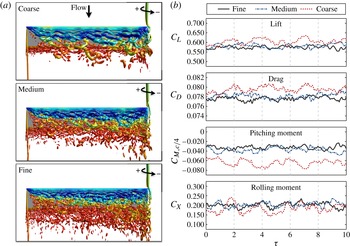
Effects of spatial resolution on the instantaneous solution for a tip-aligned impinging vortex (
 ${\rm\Delta}y=0$
). (a)
 $Q$
-criterion isosurfaces (
 $Q=15$
, coloured by pressure); (b) the unsteady lift, drag, pitching-moment and rolling-moment coefficients.

Wall-normalized mesh spacings and time step measured at
 $x/c=0.8$
along the wing’s mid-span.

For each resolution, the wall-normalized spacings in the normal direction are less than 1, the streamwise values are less than 20, and the spanwise spacings are less than 40, which all fall within the traditional bounds of LES as recommended by Georgiadis, Rizzetta & Fureby (Reference Georgiadis, Rizzetta and Fureby2010). The temporal resolution also produces values of
 ${\rm\Delta}{\it\tau}^{+}<0.006$
for each mesh, which is well below the suggested bound of 0.4 by Choi & Moin (Reference Choi and Moin1994) to properly resolve the relevant scales of fully turbulent channel flow and should adequately maintain the
 $O(1)$
viscous time scale in the boundary layer (Georgiadis et al.
Reference Georgiadis, Rizzetta and Fureby2010). The selected time step also leads to a Courant–Friedrichs–Lewy (CFL) number of
 $N_{CFL}=0.11$
based on the minimum streamwise spacing and a velocity of unity, which is a highly conservative estimate and, therefore, should ensure proper temporal resolution is maintained.
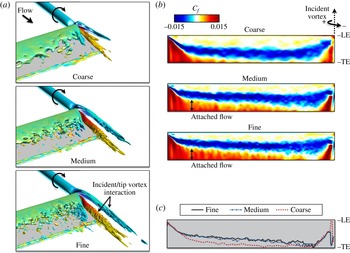
The instantaneous flow structure and loading are compared in figures 4(a) and (b), respectively. As the spatial resolution is increased, higher wavenumber modes are evident in the separated shear layer off the leading edge, as it rolls into discrete vortices that become susceptible to Kelvin–Helmholtz instabilities and transition into the wake. The smaller scales are also visible in the interaction of the tip and incident vortices at the two higher spatial resolutions, but the reduced resolution of the coarse grid does not support these higher modes. The instantaneous loading in figure 4(b) shows a collapse with increased resolution, with similar fluctuations around the same mean and only minor phase differences.
Effects of spatial resolution on the time-mean solution for a tip-aligned impinging vortex (
 ${\rm\Delta}y=0$
). (a)
 $Q$
-criterion isosurfaces (
 $Q=5$
, coloured by streamwise vorticity); (b) skin friction contours on the suction side of the wing; (c) the accompanying attachment lines on the surface.

Time-mean quantities are presented in figure 5(a–c) for each resolution. The
 $Q$
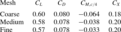
-criterion isosurfaces in figure 5(a) reveal the average interaction of the tip and incident vortices, whereby the incident vortex is deflected over the suction side of the wing from the upwash of the tip vortex. The tip and incident vortex cores remain distinct but attenuate into the wake as they entrain opposite-signed vorticity from the disrupted shear layers of the other structure, which was seen in the instantaneous solution of figure 4(a). The dissipation of either structure is less dramatic with spatial resolution, as the smaller scales are captured and provide a natural mechanism to diminish the larger shear layer vortices, thereby reducing their influence in the interaction region. Contours of skin friction on the suction side of the wing are shown in figure 5(b) along with the corresponding surface reattachment lines in figure 5(c). The skin friction distributions and reattachment lines of the medium and fine resolutions are almost indistinguishable, indicating that the relevant transitional scales have been resolved. The coarse resolution, on the other hand, leads to a larger separated region across the entire span, with reattachment occurring much closer to the trailing edge, allowing very little attached flow to remain on the wing’s surface. The time-mean loads are listed in table 4 and show a collapse with grid refinement. The weak dependence of the instantaneous and time-mean quantities on spatial resolution between the medium and fine meshes provides confidence in the fine resolution, which is used for the remainder of this study.
Mean lift, drag, pitching-moment and rolling-moment coefficients for the different spatial resolutions.

4. Results
In this section, simulations of the vortex/surface interaction are presented for various spanwise positions of the incident vortex. In all cases, the solution is initialized at free stream conditions and advanced at a constant dimensionless time step of
 ${\rm\Delta}{\it\tau}=1.0\times 10^{-4}$
for forty convective times to eliminate spurious transients associated with the startup and to allow the incoming vortex to convect past the wing and establish the flow. Ten more convective times are then simulated to collect time-mean and statistical information. As with the previous section, the chosen temporal resolution results in a wall-normalized time step in the transitional region of
 ${\rm\Delta}{\it\tau}^{+}<0.01$
for all cases, which is well below the recommended bound of 0.4 for turbulent channel flow (Choi & Moin Reference Choi and Moin1994) and should adequately maintain the
 $O(1)$
viscous time scale in the boundary layer (Georgiadis et al.
Reference Georgiadis, Rizzetta and Fureby2010).
4.1. Description of the three-dimensional flow structure
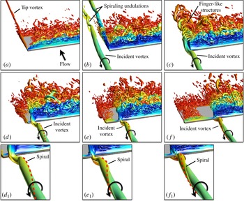
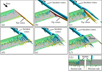
Snapshots of the instantaneous flow structure are shown in figure 6 through isosurfaces of the
 $Q$
-criterion (
 $Q=15$
). The baseline case with no vortex is shown in figure 6(a) along with all the incident vortex positions figure 6(b–f) corresponding to
 ${\rm\Delta}y=-0.25$
, 0, 0.25, 0.50 and 1.00, respectively. Additionally, the time-mean flow structure is provided in figure 7 for
 $Q=5$
. Note that the orientations between these figures differ to expose the interesting features in each.
Instantaneous isosurfaces of the
 $Q$
-criterion (
 $Q=15$
). (a) No vortex; (b)
 ${\rm\Delta}y=-0.25$
; (c)
 ${\rm\Delta}y=0.00$
; (d)
 ${\rm\Delta}y=0.25$
; (e)
 ${\rm\Delta}y=0.50$
; (f)
 ${\rm\Delta}y=1.00$
. Additional details of the impingement are provided as insets for (d–f) denoted with subscript 1.

Time-averaged isosurfaces of the
 $Q$
-criterion
 $(\overline{Q}=5)$
. (a) No vortex; (b)
 ${\rm\Delta}y=-0.25$
; (c)
 ${\rm\Delta}y=0$
; (d)
 ${\rm\Delta}y=0.25$
; (e)
 ${\rm\Delta}y=0.50$
; (f)
 ${\rm\Delta}y=1.00$
.

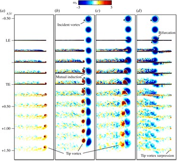
When the incident vortex is positioned just outboard of the wingtip (b), its core remains mostly undisturbed as it convects past the tip vortex. The close proximity of the two structures allows them to pair and form a vortex dipole that propels itself upwards, away from the plate through mutual induction. Although the individual vortices remain distinct and coherent in both the time-mean and instantaneous solutions, the persistent interaction promotes spiralling disruptions in their cores downstream of the wing, which can be seen in the instantaneous flow of figure 6(b).
When the incident vortex is, instead, aligned directly with the wingtip (c), it is drawn to the upper side of the wing from the accelerating flow over the leading edge and wingtip, and its outer shear layer interacts strongly with the feeding sheet of the tip vortex. Finger-like substructures develop from the swirling interaction with the leading edge and wingtip that become entrained into the tip vortex, which is of opposite-signed vorticity. While neither core is discernible in the instantaneous flow (figure 6 c), the conglomeration of all the small scales in the time-mean solution of figure 7(c) shows two distinct and coherent cores that remain intact across the wing. However, both structures attenuate into the wake from the instabilities arising within their respective feeding sheets and the entrainment of opposite-signed vorticity.
Finally, inboard positioning of the incoming vortex is shown in (d–f), and yet another, completely different regime is encountered. The upstream influence of the wing promotes spiralling disruptions in the incident vortex that wind in a direction opposite to the sense of rotation of the vortex, as pointed out in the instantaneous flow of figure 6(
 $\mathit{d}_{1}{-}\mathit{f}_{1}$
). As the incident vortex approaches the wing, the evolving spiral reorients the structure from streamwise to plate-normal, allowing it to pinch off at the leading edge, as shown in instances (a–c) of figure 8 for
 ${\rm\Delta}y=1.0$
. The downstream portion of the vortex attaches itself to the upper surface of the wing, while the remaining upstream portion is diverted to the underside and attaches to the lower surface. This underside component continues to convect and spiral until it again reorients itself perpendicular to the leading edge, as shown in instances (d) and (e) of figure 8, forcing it to pinch off in an alternate fashion as before: the downstream component attaches itself to the underside of the wing, while the remaining upstream component is diverted above the wing, anchoring itself back to the upper surface. In the time-mean solutions of figure 7(d–f), the alternating lower/upper surface deflection and attachment appears as a vortex bifurcation with portions of the incoming vortex convecting over each side of the wing. Downwash present near the wingtip for the inboard cases, reduces the effective angle of attack outboard of impingement, causing the flow to mostly attach. Two nearly identical separation bubbles are present on either side of the wing that essentially suppress the tip vortex formation in the time-mean solution (shown in inset (
 $\mathit{f}_{1}$
) of figure 7 for
 ${\rm\Delta}y=1.0$
), highlighting the reduced effective angle of attack. The other inboard positions have similar features, just over a shorter spatial extent, so they are not shown in detail.
Induced spiral of the incident vortex impinging upon the wing’s leading edge for
 ${\rm\Delta}y=1.0$
. (a,b) Upper side deflection; (c) pinch-off; (d,e) lower side deflection.

Time-mean streamwise vorticity contours dissecting the incident vortex near the wingtip. (a) No vortex; (b)
 ${\rm\Delta}y=-0.25$
; (c)
 ${\rm\Delta}y=0$
; (d)
 ${\rm\Delta}y=1.00$
. Two positions between (c) and (d) have been excluded due to their similarity to (d).

Next, the incoming vortex is dissected and shown through contours of time-mean streamwise vorticity in figure 9 as it interacts with the wing. The view is directed from a downstream location towards the inflow boundary, and the incoming vortex in each image has negatively signed (blue) vorticity. The slices start
 $0.5c$
upstream of the wing and end
 $1.5c$
into the wake. Two inboard positions have been excluded in this figure due to their similarity to (d). With outboard positioning, the vortex dipole is seen very clearly in (b) along with an enhancement of the tip vortex over the baseline case that is propelled upwards slightly, away from the surface due to the induced velocity of the pair. Both structures persist into the wake without noticeable decay. For the tip-aligned case (c), the tip and incident vortex cores are distinct, and the tip vortex (or conglomeration of the smaller scales associated with the tip vortex) is larger than that of the baseline and outboard-positioned cases. The two structures are still evident
 $1.5c$
downstream, but they experience a loss of strength and coherency as they continue to interact. Finally, with all inboard positions of the incident vortex (d), the bifurcation is quite evident along with the suppression of the tip vortex. The integrity of the incident vortex is lost as it convects downstream following its interaction with the three-dimensional recirculation region where flow is drawn inboard, and the streamwise vorticity is entrained spanwise.
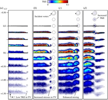
Turbulent kinetic energy contours dissecting the incident vortex near the wingtip. (a) No vortex; (b)
 ${\rm\Delta}y=-0.25$
; (c)
 ${\rm\Delta}y=0$
; (d)
 ${\rm\Delta}y=1.00$
. Two positions between (c) and (d) have been excluded due to their similarity to (d). A single contour line of time-averaged streamwise vorticity,
 $|{\it\omega}_{x}=2.0|$
, is also overlaid to highlight the tip and incident vortices.

Further insights into the unsteady interactions and vortex attenuation are provided in figure 10 through contour slices of the turbulent kinetic energy. A single contour line of the time-averaged streamwise vorticity is also overlaid to show the relative position of the incident and tip vortices. The baseline wing, figure 10(a), produces a tip vortex with very low stresses even into the wake. With outboard positioning, figure 10(b), the mutual induction of the tip/incident vortex pair is evident as both structures remain coherent but do show increased stresses in their respective cores – especially into the wake, where the spiralling disruptions became apparent from the instantaneous flow of figure 6(b). As with all vortex positions, the increased inboard separation induced by the upwash of the incident vortex is evident by the increased turbulent fluctuations off the surface of the wing and into the wake. Increased stresses are also seen in the incident vortex upstream of the wing as the spiralling instability arises farther upstream. The attenuation of the tip-aligned and tip vortices is quite apparent in figure 10(c) by the enhanced mixing of either structure into the wake as they interact and breakdown. Likewise, the inboard-positioned vortex is quickly lost in the separated region, while turbulent fluctuations also appear on the underside of the wing from the incident vortex alternating attachment and deflection.
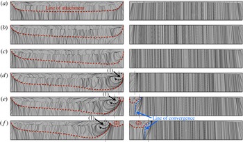
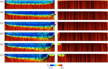
Surface-restricted streamlines from the time-mean solution: suction side (left); pressure side (right). (a) No vortex; (b)
 ${\rm\Delta}y=-0.25$
; (c)
 ${\rm\Delta}y=-0.25$
; (d)
 ${\rm\Delta}y=0.25$
; (e)
 ${\rm\Delta}y=0.50$
; (f)
 ${\rm\Delta}y=1.00$
.

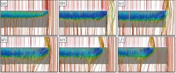
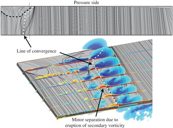
In figure 11, the surface-restricted streamlines are pictured on the suction and pressure sides of the wing. Slightly inboard-directed streamlines are seen near the impingement on the suction side of the wing for the cases in figure 11(d–f) resulting from the incident vortex interacting with its reflected image in the surface. On the underside, the lower portion of the bifurcated vortex also interacts with its image, and the induced velocity is directed outboard. In all cases, the reattachment line on the suction side of the wing (approximately shown with a dotted line) moves towards the trailing edge due to the increased separation from the upwash of the incident vortex. For all inboard positions, figure 11(d–f), the increased effective angle of attack enhances the recirculation region created by the separated boundary layer inboard of impingement that closely resembles the flow over the corner of a wing at much higher angles of attack in a free stream, which have been simulated and shown in detail by Visbal & Garmann (Reference Visbal and Garmann2012), for example, for lower-aspect-ratio wings. The incident vortex becomes entrained in this three-dimensional region and fluid is drawn inboard, thereby diminishing but not completely eliminating its impact on the outboard section of the wing. The three-dimensional streamlines over the suction side of the wing are depicted in figure 12. These images show, perhaps more clearly, the enhancement of the recirculation region that draws the fluid towards mid-span and the reduced impact outboard of impingement. It is interesting to note the almost self-similarity about these recirculation regions with inboard vortex position that appears to pin the flow near impingement and effectively reduces the usable aspect ratio of the wing. This process should eventually saturate for large enough span. The downwash that remains near the wingtip substantially reduces separation on the upper side of the wing outboard of impingement, and the reduced effective angle of attack also causes the flow on the underside to separate, as clearly indicated by the separation bubble seen in the surface-restricted streamlines in figure 11(f) denoted by (2); although the development of the separation bubble is somewhat constrained by the limited span outboard of impingement. Additionally, cases (e) and (f) show a line of convergence oriented chordwise on the underside that corresponds with a region of minor separation due to an eruption of secondary vorticity from the surface, as highlighted in figure 13 for
 ${\rm\Delta}y=1.00$
.
Three-dimensional streamlines over the suction side of the wing. (a) No vortex; (b)
 ${\rm\Delta}y=-0.25$
; (c)
 ${\rm\Delta}y=-0.25$
; (d)
 ${\rm\Delta}y=0.25$
; (e)
 ${\rm\Delta}y=0.50$
; (f)
 ${\rm\Delta}y=1.00$
.

Contours of streamwise vorticity showing the separation on the underside of the wing for
 ${\rm\Delta}y=1.00$
.

Next, the time-averaged surface pressure near the impingement location is shown in figure 14 along with the surface-restricted streamlines for each case. The incident vortex induces larger separated regions that provide more suction over a larger chordwise extent of the wing. In figure 14, the outboard (b) and tip-aligned (c) positions both reveal a stronger imprint of the tip vortex in the surface pressure (denoted as (1)) as a result of the strengthened tip vortex feeding sheet from the upwash of the incident vortex that is in close proximity. Alternatively, the incident vortex, when positioned inboard, figure 14(d–f), does not enhance the tip vortex, but instead suppresses its formation by reducing the effective angle of attack outboard of impingement. This results in two small separation bubbles on the upper and lower surfaces with nearly equivalent suction for the inboard positions examined.
Contours of surface pressure: suction side (left); pressure side (right). (a) No vortex; (b)
 ${\rm\Delta}y=-0.25$
; (c)
 ${\rm\Delta}y=0.00$
; (d)
 ${\rm\Delta}y=0.25$
; (e)
 ${\rm\Delta}y=0.50$
; (f)
 ${\rm\Delta}y=1.00$
.

Contours of the mean-squared fluctuations of pressure,
 $\overline{p^{\prime }p^{\prime }}$
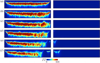
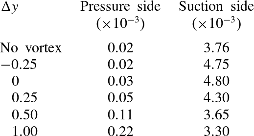
, on the surface are displayed in figure 15, and the mean values integrated over the wing are listed in table 5. On the suction side, all cases produce fluctuations across a wider chordwise extent over the baseline simulation due to the increased separation. As the vortex is moved inboard, the mean fluctuations in figure 15 decrease on the suction side from the growing region of attached flow present outboard of the impingement location, with the two farthest inboard positions,
 ${\rm\Delta}y=0.5$
and 1.0, achieving mean fluctuations below the baseline wing. Alternatively, the underside fluctuations, although much smaller than the upper side values, increase with inboard position from the portion of the bifurcated incident vortex travelling across the pressure side and disturbing the otherwise attached boundary layer. There are also fluctuations associated with reattachment of the outboard separation bubbles on either sides of the wing, as should be expected.
Contours of mean-squared fluctuations of surface pressure: suction side (left); pressure side (right). (a) No vortex; (b)
 ${\rm\Delta}y=-0.25$
; (c)
 ${\rm\Delta}y=0$
; (d)
 ${\rm\Delta}y=0.25$
; (e)
 ${\rm\Delta}y=0.50$
; (f)
 ${\rm\Delta}y=1.00$
.

Integrated surface pressure fluctuations.

4.2. Analysis of the spiralling mode instability
The spiralling core that is observed in the instantaneous solution is most obvious with inboard positioning of the incident vortex due to the strong impact with the leading edge; however, spiralling disruptions also occur with tip-aligned and outboard positioning, just at locations downstream of the leading edge. To analyse this unstable mode further, several time-histories of the velocity fluctuations in the vortex core have been gathered upstream of the wing (
 $0.5c$
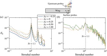
) for all cases and just off the surface at the mid-chord and inline with the impingement for all inboard positions. The power spectral density of the turbulent kinetic energy is computed from these quantities and is presented in figure 16 for each probe location. Upstream of the wing, all vortices exhibit a dominant frequency of
 $\mathit{St}=fc/U_{\infty }=1.1$
and several lower-power harmonics associated with low-wave perturbations of the core. This discrete frequency is likely a character of the chosen
 $q$
-vortex, i.e. size and strength, as it appears regardless of position. The probes just off the wing’s surface for the inboard-positioned vortices also show the same frequency from the upper/lower surface interaction, although it is less dominant as it is accompanied with fluctuations due to separation, reattachment and transition of the boundary layer.
Turbulent kinetic energy spectra,
 $E_{k}$
, aligned with the incoming vortex measured (a)
 $0.5c$
upstream of the wing and (b) just above the surface at mid-chord.

Despite all vortices exhibiting this frequency upstream of the wing, the instability is amplified and grows more quickly with inboard positioning of the vortex, which is shown by the swirl parameter decay of figure 17. Here, the evolving swirl parameter,
 $q(x)=1.567V_{0}(x)/{\rm\Delta}u(x)$
, which relates the maximum tangential velocity (
 $V_{0}(x)$
) to the axial deficit (
 ${\rm\Delta}u(x)$
) at each streamwise station, is computed from the inflow to the wing for the various vortex positions. All cases show the same natural viscous decay from the inflow but start to deviate with inboard positioning as the vortex core is subjected to more of the adverse pressure gradient associated with the stagnation on the underside of the wing. This slows the axial velocity (or increases the axial deficit), leading to an abrupt drop in the swirl parameter. For all inboard positions, and even the tip-aligned case, the swirl parameter drops below the theoretical stability threshold of the
 $q$
-vortex,
 $\sqrt{2}$
, just upstream of the leading edge, which amplifies the small-wave fluctuations, giving rise to the spiralling mode observed in the instantaneous flow structure. The swirl parameter of the outboard-positioned vortex does not drop below the stability threshold ahead of the wing, and actually shows a slight augmentation of stability as the core enjoys some benefit of the favourable pressure gradient above and outboard of the wingtip, promoting minor acceleration of the core axial flow. Farther downstream, however, as the vortex interacts with the tip vortex, the unsteady fluctuations are amplified, likely due to the shearing of the vortex dipole, leading to the spiralling disruptions seen in the wake of the instantaneous flow.
Decay of the time-mean swirl parameter,
 $q=1.567V_{0}/{\rm\Delta}u$
, as the incident vortex approaches the wing.

4.3. Aerodynamic loads
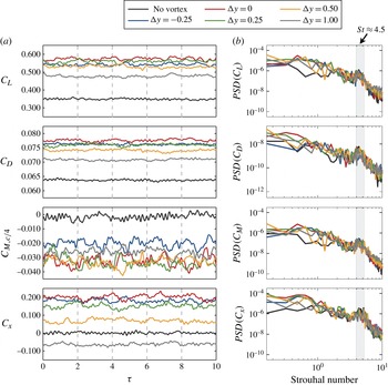
Figure 18(a) details the instantaneous force and moment histories over 10 convective times of the incident vortex interaction for each spanwise position. The clean configuration case is also shown. For all incident vortex locations, sustained increases are observed in the lift and drag coefficients, with no significant variations from their respective means. The pitching moment,
 $C_{M,c/4}$
, decreases to become more pitch-down and shows some temporal variation, most likely due to fluctuations in the larger separated region. The rolling-moment coefficient,
 $C_{X}$
, highlights a different behaviour, however. As the impingement location is moved inboard of the tip, the rolling moment decreases and eventually switches from positive to negative for
 ${\rm\Delta}y=1.0$
. Additionally, the power spectral density of the force and moment coefficients are presented in figure 18(b). The only noticeable departure from the clean wing configuration comes in the form of slightly additional power in the lowest frequencies, indicating that the unsteady interaction near the wingtip minimally affects the fluctuations observed in the integrated loads. All cases do exhibit a narrow band of frequencies centred about
 $\mathit{St}=4.5$
, corresponding to the shedding frequency of the discrete vortices formed from roll-up of the shear layer as they interact with the wing’s upper surface.
Instantaneous aerodynamic loading and spectral content for various incident vortex positions. (a) Instantaneous lift, drag, pitching-moment and rolling-moment coefficients; (b) force and moment power spectral density.

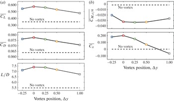
The time-mean aerodynamic loads and moments are plotted in figure 19, and the individual values are listed in table 6 for each spanwise position of the incident vortex. The baseline wing produces mean pitching and rolling moments that are essentially zero. In all cases, there is a substantial augmentation of lift and drag over the baseline wing, with the peak loads achieved when the incident vortex is aligned with the wingtip (
 ${\rm\Delta}y=0$
). This is also true with the lift-to-drag ratio, which achieves an up to 35 % increase over the baseline wing when the incident vortex is aligned with the tip. The loss of lift as the vortex moves inboard is attributed to the unloading of the tip outboard of impingement, which had been described previously and shown in the surface pressure from figure 14. The pitching moment,
 $C_{M,c/4}$
, is pitch-down for all cases, but is significantly higher in magnitude with an incoming vortex, although it does not vary dramatically with spanwise position of the incident vortex position. This, again, highlights the increased separation induced by the upwash of the vortex that moves the aerodynamic centre farther downstream of the quarter-chord position. The rolling moment, on the other hand, shows significant changes with spanwise position of the incident vortex and even changes sign as the vortex moves inboard from
 ${\rm\Delta}y=0.5$
to 1.0 as a result of the unloaded tip. This indicates that, although the tip-aligned case may be optimal for maximum achievable lift-to-drag ratio, a more inboard position may be more suitable for optimal trimming of the aircraft to reduce or even eliminate rolling moment while still seeing benefits in aerodynamic performance.
Time-mean lift, drag, pitching and rolling-moment coefficients, and lift-to-drag ratio for various incident vortex spanwise positions. The loads for the baseline case with no incident vortex are also shown (dashed lines).

Time-mean aerodynamic loads.

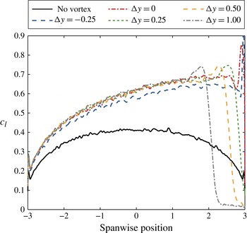
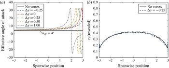
The sectional lift distribution across the span for each incident vortex position is shown in figure 20. Significant increases are observed across the entirety of the wing for each case when compared to the baseline wing with a peak encountered just inboard of the impingement location where the maximum swirl velocity occurs. The inboard positions all show the tip unloaded outboard of impingement, which was discussed earlier. The effective angle attack variation based on the prescribed inflow of the incident vortex is plotted in figure 21(a) and is computed as
 $$\begin{eqnarray}{\it\alpha}_{eff}={\it\alpha}+\tan ^{-1}(w/u_{x}),\end{eqnarray}$$
where
 ${\it\alpha}=4^{\circ }$
is the geometric angle of attack of the wing, and
 $w$
and
 $u_{x}$
are the vertical and axial velocities of the incoming vortex, respectively. The vertical velocity is given as
 $w=u_{{\it\theta}}(y-y_{c})/r$
, where
 $y$
is the spanwise position,
 $y_{c}$
is the vortex impingement location and
 $u_{{\it\theta}}$
is the circumferential velocity. Assuming the lift is proportional to the effective angle of attack by inviscid theory, the lift distribution can be rescaled by
 ${\it\alpha}/{\it\alpha}_{eff}$
, as demonstrated in figure 21(b) for the outboard-positioned incident vortex, where the effective angle of attack is well behaved and below 20°. The other positions do not collapse to the baseline case when scaled the same way, indicating that inviscid theory does not hold for the tip-aligned and inboard-positioned incoming vortices. While the side of the wing opposite impingement may see gains due to inviscid arguments, the enhancement of the recirculation region from the separated boundary layer near impingement, the reoriented spanwise flow, and the unloading of the wingtip is a viscous and highly three-dimensional process that is not properly represented by inviscid theory.
Time-mean distribution of the sectional lift coefficient for various incident vortex locations.

(a) Time-mean effective angle of attack and (b) the sectional lift coefficient rescaled by
 ${\it\alpha}/{\it\alpha}_{eft}$
for the outboard-positioned incident vortex.

5. Conclusions
High-fidelity simulations of a streamwise-oriented vortex impinging upon a finite wing have been conducted to characterize the unsteady modes of interaction. An aspect-ratio-size wing oriented at an angle of
 ${\it\alpha}=4^{\circ }$
and operating at a Reynolds number of
 $\mathit{Re}=20\,000$
was simulated with the addition of an analytically defined vortex superimposed in its free stream as a canonical problem of the vortex/surface interaction. Several spanwise positions of the incoming vortex were analysed and three distinct flow behaviours were observed.
When the vortex was positioned outboard of, but in close proximity to, the wingtip, it paired with the tip vortex to form a dipole that propelled itself upwards, away from the plate through mutual induction as both structures persisted into the wake. With tip-aligned positioning, the tip vortex was initially enhanced by the incoming vortex, but both structures attenuated into the wake as the swirling incident vortex at the leading edge led to shear layer instabilities becoming entrained into the opposite structure. Finally, when the incident vortex was positioned inboard of the wingtip, a spiralling mode was induced in its core upstream of the wing that reoriented the vortex as it impacted the leading edge, allowing it to pinch off with an alternating attachment and deflection to the upper side then the lower side of the wing. This alternating surface attachment/deflection appeared as a vortex bifurcation in the time-mean sense, with the incoming structure splitting and passing over both sides of the wing. The upwash from the incoming vortex increased the effective angle of attack inboard of impingement, which enhanced the three-dimensional recirculation region created by the separated boundary layer off the leading edge of the wing. Fluid was then drawn inboard from the incoming structure, thereby diminishing, but not completely eliminating, its impact on the outboard section of the wing. The slight downwash remaining outboard of impingement reduced the effective angle of attack, resulting in small separation bubbles on either side of the wing, and virtually suppressed the tip vortex formation for all inboard cases. The nearly symmetric formation on the upper and lower surfaces effectively unloaded the wingtip outboard of impingement, which reduced lift, drag and the incurred rolling moment. The different inboard positions created an almost self-similar flow pattern that enhanced the recirculation region, pinned the flow near impingement, and essentially reduced the usable aspect ratio of the wing by unloading the tip. This viscous and highly three-dimensional process should eventually saturate with large enough span.
Upstream of the wing, all incident vortices were shown to exhibit the same low-wave fluctuations in their respective cores at a discrete frequency of
 $\mathit{St}=1.1$
, which is believed to be a character of the chosen vortex size and strength. Tip-aligning and inboard positioning exposed the incoming structure to a stronger adverse pressure gradient on the underside of the wing that slowed the axial core velocity and thereby diminished its swirl number to a point at which this disturbance was amplified until it manifested as the spiralling mode. The outboard-positioned vortex did not reach an unstable swirl parameter upstream of the wing, but did become susceptible to spiralling disruptions farther downstream, likely due to a shearing instability from its pairing and persistent interaction with the tip vortex.
Finally, all incident vortex positions provided substantial increases in the wing’s lift-to-drag ratio; however, significant sustained rolling moments also resulted. As the vortex was brought inboard, the rolling moment diminished and eventually switched sign as the reduced outboard loading balanced the augmented sectional lift inboard of impingement.
Acknowledgements
This work is supported in part by AFOSR under a task monitored by Dr D. Smith and also by a grant of HPC time from the DoD HPC Shared Resource Centers at AFRL and ERDC.