1. Introduction
Studying the dispersion of solute transport in fluid and porous media is a crucial aspect of applied science and engineering. This process plays a vital role, among others, in effectively extracting crude oil from petroleum reservoir rocks, evaluating environmental risks and treating groundwater. Another area of interest is the spreading of aerosols, which are tiny dust particles floating in the air that can cause harm to human health. Dispersion through porous media is particularly relevant in addressing various challenges, including radioactive and reclaimed sewage disposal into aquifers, fertiliser movement in soil/groundwater, blood flow through capillaries, micro-fluidic systems, biomedical flows and lab-on-a-chip devices. Through the analysis of solute transport, we can gain insights into the complex mechanisms that occur at the micro-scale level, including diffusion, advection and dispersion. In fluids, dispersion refers to the spreading of a substance (such as solute, particle or contaminant) through a combination of fluid movement and molecular diffusion. Diffusion is the process by which particles (such as molecules or atoms) move from an area of higher concentration to the lower concentration, driven by their random motion. This movement continues until the particles are evenly distributed throughout the space, resulting in an equilibrium. Knowledge and understanding of these processes are essential for ensuring the safe and efficient use of natural resources and protecting the environment, as well as human health.
The work of Taylor (Reference Taylor1953) explored the release of passive solutes in narrow tubes, revealing that solute dispersion (named Taylor dispersion) is influenced by molecular diffusivity and non-uniform solvent velocity. Taylor’s model, expressing the diffusion coefficient, has been widely useful over time. Building upon Taylor’s findings, Aris (Reference Aris1956, Reference Aris1960) extended the analysis, introducing the concentration moment method to study solute distribution growth rate variance. They demonstrated that this variance equals the sum of Taylor and molecular diffusion coefficients. Researchers Gill & Sankarasubramanian (Reference Gill and Sankarasubramanian1970), Gill, Sankarasubramanian & Taylor (Reference Gill, Sankarasubramanian and Taylor1971) and Sankarasubramanian & Gill (Reference Sankarasubramanian and Gill1972) advanced the study of solute dispersion in fully developed, uniform and laminar flows, offering a novel approach for understanding solute behaviour in time-varying conditions. Fischer (Reference Fischer1973) explored longitudinal dispersion and turbulence mixing in open channels, while Mazumder & Das (Reference Mazumder and Das1992) investigated the impact of first-order heterogeneous reactions on dispersion in pulsating flows, noting deviations from Gaussianity due to boundary absorption effects. Hazra et al. (Reference Hazra, Gupta and Niyogi1996, Reference Hazra, Gupta and Niyogi1997) discussed solute dispersion in oscillatory flows of viscoelastic fluids, considering parameters like amplitude and pulsation frequency. Ault, Shin & Stone (Reference Ault, Shin and Stone2018) explored how particles move in narrow channels due to solute concentration gradients, focusing on diffusiophoresis and diffusioosmosis. The study develops models to control particle behaviour, with applications in particle sorting, particle concentrating and microfluidic zeta potentiometry. Shin et al. (Reference Shin, Um, Sabass, Ault, Rahimi, Warren and Stone2016) investigated solute gradient enhanced colloidal transport in dead-end channels, with larger particles concentrating more deeply due to size-dependent diffusiophoresis, useful for particle sorting and targeted drug delivery. Hinton & Woods (Reference Hinton and Woods2019) explored the depth-dependent permeability affects on tracer movement in a horizontal aquifer and showed that permeability gradients cause varying flow patterns, influencing how tracers disperse; such findings are important for understanding tracer behaviour in applications like CO2 storage. Sahu & Neufeld (Reference Sahu and Neufeld2020) examined dispersion causing fluid mixing in porous media, increasing the current’s volume over time; this study combines theory and experiments with implications for CO2 sequestration and groundwater flow.
Hydrodynamic dispersion happens in porous media, combining the molecular diffusion with variation in flow velocity through interconnected pores. The works of dispersion in porous media literature have been carried out mainly in a single-zone model. However, it occurs as a double or multilayered zone in real situations such as wetland flows, nuclear contaminant transport, etc. In their theoretical analysis, Bear (Reference Bear1961) explored anisotropic solute dispersion in porous media, emphasising the impact of flow directions and anisotropic properties. Brezinski & Buffone (Reference Brezinski and Buffone1966) conducted experiments on solute dispersion in packed beds, revealing insights into how bed characteristics influence dispersion behaviour in industrial processes. Meanwhile, Millington (Reference Millington1967) contributed a comprehensive theoretical analysis of solute dispersion in porous media, considering factors like flow velocity, diffusion coefficient and porous media properties. Bear (Reference Bear2013)’s book on solute transport in porous media covers dispersion with theoretical frameworks, mathematical models and empirical research. Cvetkovic, Dagan & Cheng (Reference Cvetkovic, Dagan and Cheng1998) extensively examined solute transport in geological formations with varying hydraulic conductivity, emphasising the effects of heterogeneity on dispersion. Cvetkovic & Dagan (Reference Cvetkovic and Dagan1994) investigated scale effects on solute dispersion in heterogeneous porous formations, quantitatively exploring the influence of varying degrees of heterogeneity on solute transport behaviour. Nield et al. (Reference Nield and Bejan2006) comprehensively covered convection in porous media, incorporating theoretical models, numerical methods and practical applications.
Beavers & Joseph (Reference Beavers and Joseph1967) contributed to fluid dynamics by investigating fluid flow in a composite region and using Darcy’s law to model the flow in porous regions. Poulikakos & Kazmierczak (Reference Poulikakos and Kazmierczak1987) conducted a study on forced convection in a partially filled duct with porous material. Kuznetsov (Reference Kuznetsov1996, Reference Kuznetsov1998) employed analytical methods to investigate fluid flow in a composite region partially filled with porous media and clear fluid. Alazmi & Vafai (Reference Alazmi and Vafai2001) explored fluid layer–porous medium interaction, considering factors such as porosity, interfacial resistance and convective heat transfer.
Minimal literature is available regarding the dispersion of solute transport in the composite region. Chen & Wu (Reference Chen and Wu2012) investigated scalar dispersion in two zone-packed regions within a tube with non-uniform flow velocity, highlighting the impact of heterogeneity on dispersion. Kumar et al. (Reference Kumar, Umavathi, Chamkha and Basawaraj2012) investigated an analytical solution for solute dispersion between two parallel plates containing porous and fluid regions, showing a decreased dispersion coefficient with higher porous parameters.
Mei, Auriault & Ng (Reference Mei, Auriault and Ng1996) introduced a multi-scale method for finding solute dispersion in single-phase fluid flows. Wu & Chen (Reference Wu and Chen2014), Wang et al. (Reference Wang, Zhu, Li and Huai2019), Barik & Dalal (Reference Barik and Dalal2019), Poddar et al. (Reference Poddar, Dhar, Mazumder and Mondal2021), Das et al. (Reference Das, Poddar, Dhar, Kairi and Mondal2021), Dhar et al. (Reference Dhar, Poddar, Mondal and Mazumder2021) used the multi-scale method to solve concentration distribution for different geometries.
No work has been found using the multi-scale method for finding solute dispersion in a two-layered channel flow. Our study introduces several novel contributions to the field of fluid flow and solute dispersion in the composite media. We extend Taylor’s classical dispersion theory, which is typically applied to single-phase flow in homogeneous tubes, to a dual-layered channel flow. The paper’s objectives focus on analysing solute movement in a two-layered channel. These objectives include:
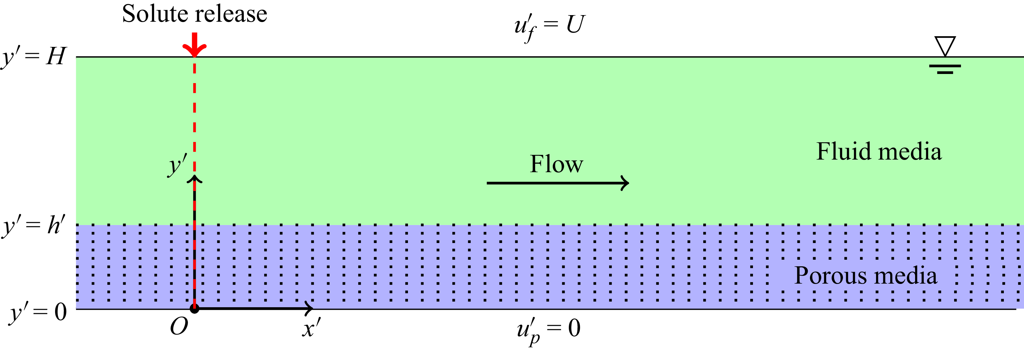
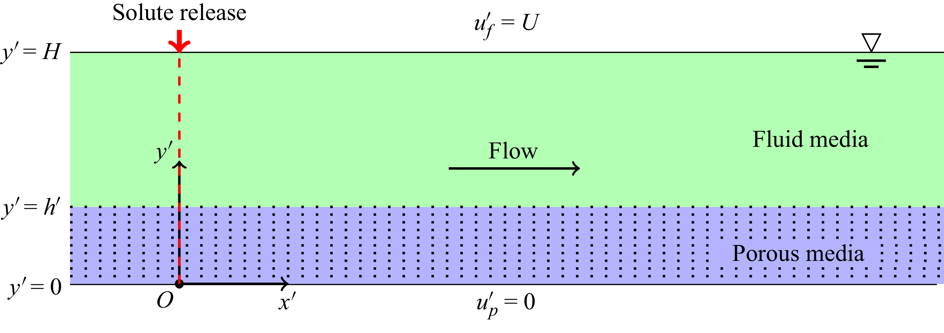
Sketch for the instantaneous release of solute in a two-layered channel.
-
(i) finding the Taylor dispersivity in the channel using perturbation analysis techniques;
-
(ii) analysing the impact of diverse flow conditions, channel properties and additional factors on solute particle dispersion;
-
(iii) determining the mean concentration and two-dimensional concentration distribution of solutes in the channel, which is crucial to comprehending solute transport;
-
(iv) demonstrating the correlations between mean solute concentrations and various parameters, such as Darcy number, pressure gradient, height of the porous region and the Péclet numbers;
-
(v) validating the results of the analytical studies with those obtained by computational studies;
-
(vi) analysing both the classical Darcy and extended Darcy models to determine which model is more appropriate. The multi-scale method provides an analytical solution for two-layered channel flow with multiple applications. These include understanding the dispersion and conveyance of contaminants in subsurface water-bearing geological formations, soil remediation, subsurface oil spills and the movement of pollutants in groundwater resources. A real-life application of these findings can be seen in groundwater contamination scenarios, where stratified aquifers necessitate predictions of contaminant behaviour; using our derived models, environmental engineers can assess solute dispersion, leading to improved remediation strategies to protect water quality.
2. Formulation of the problem
This study focuses on analysing a unidirectional fully developed flow within a two-layered channel possessing a distinctive configuration. The channel of width
 $H$
comprises of two distinct layers: an upper layer filled with fluid having a free surface and a lower layer permeated by a porous medium with uniform permeability. In order to ensure a precise analysis of the solute transport phenomenon, specific fundamental assumptions and conditions are employed, which have been explained below.
Firstly, velocity continuity is imposed, which mandates that the fluid’s velocity remains uniform throughout the interface separating the two layers. This stipulation guarantees that the fluid velocity in the lower layer, which is a porous medium, is equivalent to the fluid velocity at the free surface in the upper layer and that this equivalence occurs at their interface. Moreover, a no-slip boundary condition is enforced at the impermeable wall, typically located at the bottom of the lower layer.
Figure 1 depicts a schematic diagram of the problem. The fluid motion in the porous region is governed by the extended Darcy equation (Vafai & Kim Reference Vafai and Kim1990, Reference Vafai and Kim1995)
 \begin{equation} -\dfrac {{\rm d}p}{{\rm d}x'} +\mu _{e}\dfrac {{\rm d}^2u^{\prime}_{\!p}(y')}{{\rm d}y'^2} -\mu \frac {u^{\prime}_{\!p}(y')}{\kappa } = 0,\quad 0 \leqslant y' \leqslant h', \end{equation}
and the fluid motion in the fluid region is governed by the Stokes equation (Kuznetsov Reference Kuznetsov1998)
 \begin{equation} - \dfrac {{\rm d}p}{{\rm d}x'} +\mu \dfrac {{\rm d}^2u^{\prime}_{\!f}(y')}{{\rm d}y'^2} = 0,\quad h' \leqslant y' \leqslant H, \end{equation}
where
 $u^{\prime}_{\!p}(y')$
and
 $u^{\prime}_{\!f}(y')$
are fluid velocities in the porous region and fluid region, respectively,
 $ \kappa$
is the permeability of the porous medium and
 $h'$
is the thickness or depth of the porous layer;
 $ \mu$
is the fluid viscosity and
 $\mu _e$
is the effective viscosity representing an apparent viscosity that includes the resistance effects from porous media or complex flow conditions. It varies based on factors like porosity and permeability and is generally higher than dynamic viscosity, which is the inherent resistance of a pure fluid to flow. Both share the same units, but effective viscosity adjusts for environmental factors, making it a variable property (Givler & Altobelli Reference Givler and Altobelli1994, Martys, Bentz & Garboczi Reference Martys, Bentz and Garboczi1994). The pressure gradient
 $(- {{\rm d}p}/{{\rm d}x'})$
in (2.1) and (2.2) is constant and equal (Ochoa-Tapia & Whitaker Reference Ochoa-Tapia and Whitaker1995). We mention that the use of (2.1) is sometimes questionable, however, in a recent study, Winter et al. (Reference Winter, Valsamidou, Class and Flemisch2022) showed that when the fluid from the high velocity flow region infiltrates into the porous region, the inertia effects dominate. In such cases, the Darcy-extended model would better predict results than the use of the pure Darcy model.
Consider the transport of a scalar quantity in a fully developed, unidirectional flow through a dual-layered channel, where the channel’s length is much larger than its depth, in a Cartesian coordinate system with the longitudinal
 $x'$
axis aligned with the flow direction, the
 $y'$
axis aligned with the lateral direction and the origin set at one of the channel bank walls, as shown in figure 1.
The problem of solute transport in a porous region and a fluid region can be respectively formulated as (Mei & Vernescu Reference Mei and Vernescu2010)
 \begin{align} \frac {\partial C_{\!p}^{\prime}}{\partial t'} +u^{\prime}_{\!p}(y')\frac {\partial C_{\!p}^{\prime}}{\partial x'} &= D_p\left (\frac {\partial ^2 C_{\!p}^{\prime}}{\partial x'^2} + \frac {\partial ^2 C_{\!p}^{\prime}}{\partial y'^2}\right )\!, \hspace {5mm} 0\lt y' \leqslant h', \end{align}
 \begin{align} \frac {\partial C_{\!f}^{\prime}}{\partial t'} +u^{\prime}_{\!f}(y')\frac {\partial C_{\!f}^{\prime}}{\partial x'} &= D_{\!f}\left (\frac {\partial ^2 C_{\!f}^{\prime}}{\partial x'^2} + \frac {\partial ^2 C_{\!f}^{\prime}}{\partial y'^2}\right )\!, \hspace {5mm} h'\leqslant y' \lt H, \end{align}
where
 $D_p$
and
 $D_{\!f}$
are the diffusion coefficients in the porous region and fluid region, respectively, assumed to be constants,
 $t'$
is the time, and
 $C_{\!p}(x',y',t')$
and
 $C_{\!f}^{\prime}(x',y',t')$
are the concentrations of the diffusive substance in the porous region and fluid region, respectively.
2.1. Initial and boundary conditions
The no-slip condition is applied at the bottom of the channel, i.e.
 \begin{equation} u^{\prime}_{\!p}(y') = 0 \quad \text{at} \, y'=0. \end{equation}
The continuity of the average velocity and continuity of stress jump conditions are applied at the interface as
 \begin{equation} u^{\prime}_{\!p}(y') = u^{\prime}_{\!f}(y') \quad \text{at} \, y'=h', \end{equation}
and
 \begin{equation} \mu _{e} \dfrac {{\rm d}u^{\prime}_{\!p}(y')}{{\rm d}y'} = \mu \dfrac {{\rm d}u^{\prime}_{\!f}(y')}{{\rm d}y'} \quad \text{at} \, y'=h'. \end{equation}
Here
 $U$
is the flow velocity of the free surface, i.e.
 \begin{equation} u^{\prime}_{\!f}(y') = U \quad \text{at} \,y' = H. \end{equation}
The initial conditions for the solute transport equations are
 \begin{align} C_{\!p}^{\prime}(x',y',t')\mid _{t'=0} &= \frac { Q_m\delta \left(\dfrac {x'}{H}\right)}{H},\quad 0\lt y' \leqslant h', \end{align}
 \begin{align} C_{\!f}^{\prime}(x',y',t')\mid _{t'=0} &= \frac { Q_m\delta \left(\dfrac {x'}{H}\right)}{H},\quad h'\leqslant y' \lt H, \end{align}
where
 $Q_m$
is the released mass at
 $t'=0$
and
 $\delta (\boldsymbol{\cdot })$
is the Dirac delta function.
The boundary conditions for solute transport are given as
 \begin{equation} \frac {\partial C_{\!p}^{\prime}}{\partial y'}\bigg {|} _{y'=0} = \frac {\partial C_{\!f}^{\prime}}{\partial y'}\bigg {|}_{y'=H} = 0, \end{equation}
and the symmetry condition is applied as
 \begin{equation} C_{\!p}^{\prime}\mid _{y'=h'} = C_{\!f}^{\prime}\mid _{y'=h'}, \end{equation}
and
 \begin{equation} D_p\frac {\partial C_{\!p}^{\prime}}{\partial y'}\bigg {|}_{y'=h'} = D_{\!f}\frac {\partial C_{\!f}^{\prime}}{\partial y'}\bigg {|}_{y'=h'}. \end{equation}
At significant distances the tracer concentrations are considered negligible, i.e.
 \begin{align}& C_{\!p}^{\prime}(x',y',t')\mid _{x'\rightarrow \pm \infty } = 0,\quad 0\lt y' \leqslant h', \end{align}
 \begin{align}& C_{\!f}^{\prime}(x',y',t')\mid _{x'\rightarrow \pm \infty } = 0,\quad h'\leqslant y' \lt H. \end{align}
3. Theoretical model
3.1. Dimensionless governing equations
The following dimensionless variables are introduced to make governing equations dimensionless:
 \begin{gather} x = \frac {x'}{L},\quad y = \frac {y'}{H},\quad h= \frac {h'}{H},\quad C = \frac {C'}{Q_m/H},\quad t = \frac {t'}{L/U},\quad u_p = \frac {u^{\prime}_{\!p}}{U},\quad u_{\!f} = \frac {u^{\prime}_{\!f}}{U}, \nonumber \\{\textit{Pe}}_p = \frac {U H}{D_p}, \quad {\textit{Pe}}_{\!f} = \frac {U H}{D_{\!f}}, D_a =\frac {\kappa }{H^2}, \quad Q = -\frac {{\rm d}p}{{\rm d}x'}\Big /\frac {\mu U}{H^2}, \quad M = \frac {\mu _e}{\mu }. \end{gather}
The angle bracket denotes the section average defined as
 \begin{equation} \langle u\rangle = \int _{0}^{h} u_p(y) {\rm d}y + \int _{h}^{1} u_{\!f}(y) {\rm d}y. \end{equation}
Using the dimensionless variables, we get the velocity profiles after solving (2.1) and (2.2), together with initial conditions and boundary conditions (2.5)–(2.8) as follows:
 \begin{equation} u_p(y) = \textit{QD}_a \left (1-\cosh \left \{\frac {y}{\sqrt {{\textit{MD}}_a}}\right \}\right ) +d_2\sinh \left \{\frac {y}{\sqrt {{\textit{MD}}_a}}\right \} \end{equation}
and
 \begin{equation} u_{\!f}(y) = 1- d_1(1-y) +\frac {Q}{2}\left(1-y^2\right). \end{equation}
Here
 $d_1$
and
 $d_2$
are given as
 \begin{align}&\qquad\qquad d_1 = d_2\sqrt {\frac {M}{D_a}}\cosh \left \{\frac {1}{\sqrt {{\textit{MD}}_a}}h\right \}-Q\sqrt {{\textit{MD}}_a}\sinh \left \{\frac {1}{\sqrt {{\textit{MD}}_a}}h\right \}+ hQ, \end{align}
 \begin{align}& d_2 = \frac {1+\dfrac {1}{2}Q(1-h)^2 -{\textit{QD}}_a\left (1-\cosh \left \{\dfrac {1}{\sqrt {{\textit{MD}}_a}}h\right \}\!\right ) +(1-h)Q\sqrt {{\textit{MD}}_a}\sinh \left\{\dfrac {1}{\sqrt {{\textit{MD}}_a}}h\right\}}{\sinh \left \{\dfrac {1}{\sqrt {{\textit{MD}}_a}}h\right \} + \sqrt {\dfrac {M}{D_a}}(1-h)\cosh \left \{\dfrac {1}{\sqrt {{\textit{MD}}_a}}h\right \}}. \end{align}
The dimensionless form of governing equations and initial and boundary conditions for solute transport in the porous region and the fluid region will be reduced to, respectively,
 \begin{align}& \epsilon \frac {\partial C_{\!p}}{\partial t} + \epsilon u_p \frac {\partial C_{\!p}}{\partial x} = \frac {1}{{\textit{Pe}}_p}\left(\epsilon ^2 \frac {\partial ^2 C_{\!p}}{\partial x^2} + \frac {\partial ^2 C_{\!p}}{\partial y^2}\right), \quad 0 \lt y \leqslant h,\\[-12pt]\nonumber\end{align}
 \begin{align}& \epsilon \frac {\partial C_{\!f}}{\partial t} + \epsilon u_{\!f} \frac {\partial C_{\!f}}{\partial x} = \frac {1}{{\textit{Pe}}_{\!f}}\left(\epsilon ^2 \frac {\partial ^2 C_{\!f}}{\partial x^2} + \frac {\partial ^2 C_{\!f}}{\partial y^2}\right), \hspace {5mm} h\leqslant y \lt 1,\\[-12pt]\nonumber \end{align}
 \begin{align}&\qquad\qquad\,\, C_{\!p}(x,y,t)\mid _{t=0} = \delta \left(\frac {x}{\epsilon }\right),\quad 0\lt y \leqslant h,\\[-12pt]\nonumber \end{align}
 \begin{align}&\qquad\qquad C_{\!f}(x,y,t)\mid _{t=0} = \delta \left(\frac {x}{\epsilon }\right),\quad \leqslant h \lt y \lt 1,\\[-12pt]\nonumber \end{align}
 \begin{align}&\qquad\qquad\qquad\quad \frac {\partial C_{\!p}}{\partial y}\bigg {|}_{y=0} = \frac {\partial C_{\!f}}{\partial y}\bigg {|}_{y=1} = 0,\\[-12pt]\nonumber \end{align}
 \begin{align}&\qquad\qquad\qquad\qquad C_{\!p} \mid _{y=h} = C_{\!f} \mid _{y=h},\\[-12pt]\nonumber \end{align}
 \begin{align}&\qquad\qquad\qquad \frac {1}{{\textit{Pe}}_{p}}\frac {\partial C_{\!p}}{\partial y}\bigg {|}_{y=h} = \frac {1}{{\textit{Pe}}_{\!f}}\frac {\partial C_{\!f}}{\partial y}\bigg {|}_{y=h}, \end{align}
and
 \begin{align}& C_{\!p}(x,y,t)\mid _{x\rightarrow \pm \infty } = 0,\quad 0\lt y \leqslant h, \end{align}
 \begin{align}& C_{\!f}(x,y,t)\mid _{x\rightarrow \pm \infty } = 0,\quad h\leqslant y \lt 1. \end{align}
3.2. Asymptotic analysis
The multi-scale approach is an incredibly effective methodology for tackling problems that depend on multiple scales. Employing an ‘averaging out’ process, it transforms complex microscopic equations into more manageable macroscopic ones especially for the porous region. This approach is beneficial for solving problems with significant differences in scale. Mei (Reference Mei1992), Mei et al. (Reference Mei, Auriault and Ng1996) introduced homogenisation techniques in fluid dynamics, which have provided a systematic approach for studying dispersion in single-phase fluid flows and inspired several subsequent studies such as Ng & Mei (Reference Ng and Mei1996). When examining the process of passive solute transport in a two-layered channel flow, it is necessary to consider two distinct length scales:
 $H$
, which represents the depth of the channel; and
 $L$
, which represents the characteristic longitudinal length of the solute cloud. In addition, two relevant time scales must be taken into account:
 $ T_0$
, denoting the convection time across
 $L$
, expressed as
 $T_0 = L/U$
(with
 $U$
representing free surface velocity); and
 $T_1$
, representing the diffusion time across
 $L$
, expressed as
 $T_1 = L^2/D$
(here,
 $D=D_p$
in the porous region and
 $D=D_{\!f}$
in the fluid region). Their ratio is
 $T_0:T_1 = 1:1/\epsilon$
, where
 $\epsilon \,(=H/L\ll 1)$
is the perturbation parameter that represents the relationship between the channel depth
 $H$
and the characteristic length
 $L$
. In this analysis we have considered that
 $O({\textit{Pe}}_p)=O({\textit{Pe}}_{\!f})=1$
. Based on the time scales, two-time variables,
 $t_0 = t$
and
 $t_1 =\epsilon t$
, are introduced to effectively analyse the system’s dynamics at different scales. This approach helps us to better understand the transport phenomena and allows us to create simplified macroscopic equations that are easier to analyse and solve.
The time derivative is expanded using the chain rule as (Chen & Wu Reference Chen and Wu2012)
 \begin{equation} \frac {\partial }{\partial t} = \frac {\partial }{\partial t_0}+\epsilon \frac {\partial }{\partial t_1}. \end{equation}
In multi-scale approaches the concentrations
 $C_{\!p}$
and
 $C_{\!f}$
are expanded as (Chen & Wu Reference Chen and Wu2012)
 \begin{equation} C_{\!p}(x,y,t) = C_{\!p}^{(0)}(x,y,t_0,t_1)+\epsilon C_{\!p}^{(1)}(x,y,t_0,t_1)+\epsilon ^2 C_{\!p}^{(2)}(x,y,t_0,t_1)+\ldots +O(\epsilon ^n) \end{equation}
and
 \begin{equation} C_{\!f}(x,y,t) = C_{\!f}^{(0)}(x,y,t_0,t_1)+\epsilon C_{\!f}^{(1)}(x,y,t_0,t_1)+\epsilon ^2 C_{\!f}^{(2)}(x,y,t_0,t_1)+\ldots +O(\epsilon ^n). \end{equation}
Substituting (3.16)–(3.18) into (3.7)–(3.13), the
 $O(\epsilon ^0)$
approximation is obtained as
 \begin{align}&\,\,\,\, \frac {\partial ^2 C_{\!p}^{(0)}}{\partial y^2} = 0, \quad 0\lt y \leqslant h,\\[-12pt]\nonumber \end{align}
 \begin{align}&\,\,\,\, \frac {\partial ^2 C_{\!f}^{(0)}}{\partial y^2} = 0,\quad h \leqslant y \lt 1,\\[-12pt]\nonumber \end{align}
 \begin{align}&\,\, \frac {\partial C_{\!p}^{(0)}}{\partial y}\bigg {|}_{y=0} = \frac {\partial C_{\!f}^{(0)}}{\partial y}\bigg {|}_{y=1}=0,\\[-12pt]\nonumber \end{align}
 \begin{align}&\qquad C_{\!p}^{(0)}\mid _{y=h} = C_{\!f}^{(0)}\mid _{y=h},\\[-12pt]\nonumber \end{align}
 \begin{align}& \frac {1}{{\textit{Pe}}_{p}}\frac {\partial C_{\!p}^{(0)}}{\partial y}\bigg {|}_{y=h} = \frac {1}{{\textit{Pe}}_{\!f}}\frac {\partial C_{\!f}^{(0)}}{\partial y}\bigg {|}_{y=h}. \end{align}
We can conclude that from (3.19)–(3.23),
 \begin{equation} C^{(0)}(x,t_0,t_1) = \begin{cases} C_{\!p}^{(0)}(x,t_0,t_1),\quad 0\lt y \leqslant h,\\[6pt] C_{\!f}^{(0)}(x,t_0,t_1), \quad h\leqslant y \lt 1. \end{cases} \end{equation}
Substituting (3.16)–(3.18) into (3.7)–(3.13), the
 $O(\epsilon )$
approximation is obtained as
 \begin{align}& \frac {\partial C_{\!p}^{(0)}}{\partial t_0}+u_p(y)\frac {\partial C_{\!p}^{(0)}}{\partial x} = \frac {1}{{\textit{Pe}}_{p}}\frac {\partial ^2C_{\!p}^{(1)}}{\partial y^2},\quad 0 \lt y\leqslant h, \end{align}
 \begin{align}& \frac {\partial C_{\!f}^{(0)}}{\partial t_0}+ u_{\!f}(y)\frac {\partial C_{\!f}^{(0)}}{\partial x} = \frac {1}{{\textit{Pe}}_{\!f}}\frac {\partial ^2C_{\!f}^{(1)}}{\partial y^2},\quad h \leqslant y \lt 1, \end{align}
 \begin{align}&\qquad\qquad \frac {\partial C_{\!p}^{(1)}}{\partial y}\bigg {|}_{y=0} = \frac {\partial C_{\!f}^{(1)}}{\partial y}\bigg {|}_{y=1} = 0, \end{align}
 \begin{align}&\qquad\qquad\quad C_{\!p}^{(1)}\mid _{y=h} = C_{\!f}^{(1)}\mid _{y=h}, \end{align}
 \begin{align}&\qquad\quad \frac {1}{{\textit{Pe}}_{p}}\frac {\partial C_{\!p}^{(1)}}{\partial y}\bigg {|}_{y=h} = \frac {1}{{\textit{Pe}}_{\!f}}\frac {\partial C_{\!f}^{(1)}}{\partial y}\bigg {|}_{y=h}. \end{align}
We apply the section average with respect to the spatial variable
 $y$
of (3.25) and (3.26) to obtain
 \begin{equation} \frac {\partial C^{(0)}}{\partial t_0}+\langle u\rangle \frac {\partial C^{(0)}}{\partial x} = 0. \end{equation}
Subtracting (3.30) from (3.25) and (3.26) and using the relationship (3.24), we have
 \begin{equation} \frac {\partial ^2C_{\!p}^{(1)}}{\partial y^2}={\textit{Pe}}_{p}(u_p- \langle u \rangle )\frac {\partial C^{(0)}}{\partial x},\quad 0 \lt y \leqslant h, \end{equation}
and
 \begin{equation} \frac {\partial ^2C_{\!f}^{(1)}}{\partial y^2}={\textit{Pe}}_{\!f}(u_{\!f}- \langle u \rangle )\frac {\partial C^{(0)}}{\partial x},\quad h \leqslant y \lt 1. \end{equation}
Since advection in the
 $y$
direction is negligible, this assumption allows the system to exhibit separability in
 $x$
and
 $y$
:
 \begin{align}& C_{\!p}^{(1)} = {\textit{Pe}}_{p}N_p(y)\frac {\partial C^{(0)}}{\partial x},\quad 0 \lt y \leqslant h,\\[-12pt]\nonumber \end{align}
 \begin{align}& C_{\!f}^{(1)} = {\textit{Pe}}_{\!f}N_{\!f}(y)\frac {\partial C^{(0)}}{\partial x},\quad h\leqslant y \lt 1. \end{align}
Here the transverse functions
 $N_p(y)$
and
 $N_{\!f}(y)$
can be respectively found from the equations
 \begin{align}& \frac {{\rm d}^2N_p(y)}{{\rm d}y^2} = u_p(y)-\langle u \rangle ,\quad 0 \lt y \leqslant h, \end{align}
 \begin{align}& \frac {{\rm d}^2N_{\!f}(y)}{{\rm d}y^2} = u_{\!f}(y)-\langle u\rangle ,\quad h\leqslant y \lt 1, \end{align}
with the boundary conditions
 \begin{align}&\quad\,\, \frac {\partial N_p}{\partial y}\mid _{y=0} = \frac {\partial N_{\!f}}{\partial y}\mid _{y=1}=0,\\[-12pt]\nonumber \end{align}
 \begin{align}& {\textit{Pe}}_{p}N_p(y)\mid _{y=h} = {\textit{Pe}}_{\!f}N_{\!f}(y)\mid _{y=h},\\[-12pt]\nonumber \end{align}
 \begin{align}&\qquad \frac {\partial N_p}{\partial y}\mid _{y=h} = \frac {\partial N_{\!f}}{\partial y}\mid _{y=h}, \end{align}
and the consistency condition
 \begin{equation} \langle Pe N \rangle = {\textit{Pe}}_p\int _{0}^{h} N_p(y) {\rm d}y + {\textit{Pe}}_{\!f}\int _{h}^{1} N_{\!f}(y) {\rm d}y = 0. \end{equation}
After solving (3.35) and (3.36), we get
 \begin{align} N_p(y) &= \textit{QD}_a\left \{\frac {y^2}{2}-\textit{MD}_a\cosh \left (\frac {y}{\sqrt {{\textit{MD}}_a}}\right )\right \}\nonumber\\&\quad +d_2\left \{{\textit{MD}}_a\sinh \left (\frac {y}{\sqrt {{\textit{MD}}_a}}\right ) -\sqrt {{\textit{MD}}_a}\, y\right \} -\langle u \rangle \frac {y^2}{2}+d_3 \end{align}
and
 \begin{align} N_{\!f}(y) = \left (\langle u \rangle -\frac {Q}{3}+\frac {d_1}{2}-1\right )y+\left (\frac {1}{2}-\frac {d_1}{2}+\frac {Q}{4}-\frac {\langle u \rangle }{2}\right )y^2+\frac {d_1}{6}y^3-\frac {Q}{24}y^4+d_4, \end{align}
where
 $d_3$
and
 $d_4$
are given in Appendix A and
 $\langle u \rangle$
can be found as
 \begin{align} \langle u \rangle &= \textit{QD}_a\left \{h-\sqrt {{\textit{MD}}_a}\sinh \left (\frac {h}{\sqrt {{\textit{MD}}_a}}\right )\right \} -d_2\sqrt {{\textit{MD}}_a}\left \{1-\cosh \left (\frac {h}{\sqrt {{\textit{MD}}_a}}\right )\right \}\nonumber\\&\quad +\left (1-h\right )-\frac {d_1}{2}\left (1-h\right )^2 + \frac {Q}{6}\left (2-3h+h^3\right )\!, \end{align}
where
 $d_1$
and
 $d_2$
are provided in (3.5) and (3.6), respectively.
Similarly, for
 $O(\epsilon ^2)$
approximations, we obtain
 \begin{align}& \frac {\partial C_{\!p}^{(1)}}{\partial t_0}+\frac {\partial C_{\!p}^{(0)}}{\partial t_1}+ u_p\frac {\partial C_{\!p}^{(1)}}{\partial x} = \frac {1}{{\textit{Pe}}_p}\left (\frac {\partial ^2 C_{\!p}^{(0)}}{\partial x^2}+\frac {\partial ^2 C_{\!p}^{(2)}}{\partial y^2}\right )\!,\\[-12pt]\nonumber \end{align}
 \begin{align}& \frac {\partial C_{\!f}^{(1)}}{\partial t_0}+\frac {\partial C_{\!f}^{(0)}}{\partial t_1}+ u_{\!f}\frac {\partial C_{\!f}^{(1)}}{\partial x} = \frac {1}{{\textit{Pe}}_{\!f}}\left (\frac {\partial ^2 C_{\!f}^{(0)}}{\partial x^2}+\frac {\partial ^2 C_{\!f}^{(2)}}{\partial y^2}\right )\!,\\[-12pt]\nonumber \end{align}
 \begin{align}&\qquad\qquad\qquad \frac {\partial C_{\!p}^{(2)}}{\partial y}\bigg {|}_{y=0} = \frac {\partial C_{\!f}^{(2)}}{\partial y}\bigg {|}_{y=1} = 0,\\[-12pt]\nonumber \end{align}
 \begin{align}&\qquad\qquad\qquad\quad C_{\!p}^{(2)}\mid _{y=h} = C_{\!f}^{(2)}\mid _{y=h} ,\\[-12pt]\nonumber \end{align}
 \begin{align}&\qquad\qquad\quad \frac {1}{{\textit{Pe}}_p}\frac {\partial C_{\!p}^{(2)}}{\partial y}\bigg {|}_{y=h} = \frac {1}{{\textit{Pe}}_{\!f}}\frac {\partial C_{\!f}^{(2)}}{\partial y}\bigg {|}_{y=h}. \end{align}
Substituting (3.33) and (3.34) into (3.44) and (3.45) with the help of (3.30), we get
 \begin{align}& \frac {\partial C^{(0)}}{\partial t_1} = \left \{\frac {1}{{\textit{Pe}}_p}-(u_p-\langle u \rangle ){\textit{Pe}}_{p}N_p(y)\right \}\frac {\partial ^2 C^{(0)}}{\partial x^2} +\frac {1}{{\textit{Pe}}_p}\frac {\partial ^2 C_{\!p}^{(2)}}{\partial y^2}, \quad 0 \lt y \leqslant h, \end{align}
 \begin{align}& \frac {\partial C^{(0)}}{\partial t_1} = \left \{\frac {1}{{\textit{Pe}}_{\!f}}-(u_{\!f}-\langle u \rangle ){\textit{Pe}}_{\!f}N_{\!f}(y)\right \}\frac {\partial ^2 C^{(0)}}{\partial x^2} +\frac {1}{{\textit{Pe}}_{\!f}}\frac {\partial ^2 C_{\!f}^{(2)}}{\partial y^2}, \quad h \leqslant y \lt 1. \\[9pt] \nonumber \end{align}
Using the averaging operation of (3.49) and (3.50), we have
 \begin{align}& \frac {\partial C^{(0)}}{\partial t_1} = \bigg [ \int _{0}^{h} \left \{ \frac {1}{{\textit{Pe}}_p} - {\textit{Pe}}_p \left ( u_p - \langle u \rangle \right ) N_p(y) \right \} {\rm d}y \nonumber\\ &\qquad\qquad + \int _{h}^{1} \left \{ \frac {1}{{\textit{Pe}}_{\!f}} - {\textit{Pe}}_{\!f} \left ( u_{\!f} - \langle u \rangle \right ) N_{\!f}(y) \right \} {\rm d}y \bigg ] \frac {\partial ^2 C^{(0)}}{\partial x^2}, \end{align}
 \begin{align}&\qquad\qquad\quad \frac {\partial C^{(0)}}{\partial t_1} = \left \langle \frac {1}{\textit{Pe}} -Pe u N(y)\right \rangle \frac {\partial ^2 C^{(0)}}{\partial x^2}, \\[9pt] \nonumber \end{align}
where
 \begin{equation} \begin{aligned} \left \langle \frac {1}{\textit{Pe}} - \textit{Pe}\, u\, N(y) \right \rangle &= \int _{0}^{h} \left \{ \frac {1}{{\textit{Pe}}_p} - {\textit{Pe}}_p \left ( u_p - \langle u \rangle \right ) N_p(y) \right \} {\rm d}y \\ &\quad + \int _{h}^{1} \left \{ \frac {1}{{\textit{Pe}}_{\!f}} - {\textit{Pe}}_{\!f} \left ( u_{\!f} - \langle u \rangle \right ) N_{\!f}(y) \right \} {\rm d}y. \end{aligned} \end{equation}
Multiplying (3.52) by
 $\epsilon$
and adding (3.30), we have
 \begin{equation} \frac {\partial C^{(0)}}{\partial t_0}+\epsilon \frac {\partial C^{(0)}}{\partial t_1}+\langle u\rangle \frac {\partial C^{(0)}}{\partial x} = \epsilon \left \langle \frac {1}{\textit{Pe}} -Pe u N(y)\right \rangle \frac {\partial ^2 C^{(0)}}{\partial x^2}. \end{equation}
 \begin{equation} \frac {\partial C^{(0)}}{\partial t}+ \langle u\rangle \frac {\partial C^{(0)}}{\partial x} = \epsilon \left \langle \frac {1}{\textit{Pe}} -Pe u N(y)\right \rangle \frac {\partial ^2 C^{(0)}}{\partial x^2}. \end{equation}
Using the initial and boundary conditions given in (2.9)–(2.13), the solution of (3.55) can be written in the new variables
 $t^*$
and
 $\zeta$
, where
 $x = {x'}/{L}$
,
 $t = {t'}/({{L}/{U}})$
,
 $t^*={t'}/({{H^2}/{\langle D \rangle }})$
and
 $\zeta = {x'}/{H}- {\langle u \rangle t^*}/{\langle {1}/{\textit{Pe}}\rangle }$
, as
 \begin{equation} C^{(0)} = \frac {1}{\sqrt { 4\pi D_T t^*}}\exp \left (\frac {-\zeta ^2}{4 D_T t^*}\right )\!, \end{equation}
where
 $D_T$
is the effective dispersion coefficient, which is given as
 \begin{equation} D_T = 1-\frac {\langle Pe u N(y)\rangle }{\langle \dfrac {1}{\textit{Pe}}\rangle }. \end{equation}
Here , the averages
 \begin{equation} \left \langle \frac {1}{\textit{Pe}}\right \rangle = \frac {h}{{\textit{Pe}}_p} + \frac {1-h}{{\textit{Pe}}_{\!f}} \end{equation}
and
 \begin{equation} \begin{aligned} \langle Pe\, u\, N(y) \rangle &= \int _{0}^{h} {\textit{Pe}}_p \left ( u_p - \langle u \rangle \right ) N_p(y)\, {\rm d}y + \int _{h}^{1} {\textit{Pe}}_{\!f} \left ( u_{\!f} - \langle u \rangle \right ) N_{\!f}(y)\, {\rm d}y \\ &= {\textit{Pe}}_p I_1 + {\textit{Pe}}_{\!f} I_2, \end{aligned} \end{equation}
where the parameters
 $I_1$
and
 $I_2$
are given in Appendix A.
Substituting (3.52) into (3.49) and (3.50), we get
 \begin{equation} \frac {1}{{\textit{Pe}}_p}\frac {\partial ^2 C_{\!p}^{(2)}}{\partial y^2} = \left [\left \langle \frac {1}{\textit{Pe}}-PeuN(y)\right \rangle -\left \{\frac {1}{{\textit{Pe}}_p}-{\textit{Pe}}_p(u_p-\langle u \rangle )N_p(y)\right \}\right ]\frac {\partial ^2 C^{(0)}}{\partial x^2} \end{equation}
and
 \begin{equation} \frac {1}{{\textit{Pe}}_{\!f}}\frac {\partial ^2 C_{\!f}^{(2)}}{\partial y^2} = \left [\left \langle \frac {1}{\textit{Pe}}-PeuN(y)\right \rangle -\left \{\frac {1}{{\textit{Pe}}_{\!f}}-{\textit{Pe}}_{\!f}(u_{\!f}-\langle u \rangle )N_{\!f}(y)\right \}\right ]\frac {\partial ^2 C^{(0)}}{\partial x^2}. \end{equation}
Since advection in the
 $y$
direction is negligible, this assumption allows the system to exhibit separability. Let us consider the solutions of (3.60) and (3.61) as
 \begin{equation} C_{\!p}^{(2)} = {\textit{Pe}}_pX_p(y)\frac {\partial ^2 C^{(0)}}{\partial x^2}, \quad 0\lt y\leqslant h, \end{equation}
and
 \begin{equation} C_{\!f}^{(2)} = {\textit{Pe}}_{\!f}X_{\!f}(y)\frac {\partial ^2 C^{(0)}}{\partial x^2},\quad h \leqslant y \lt 1, \end{equation}
respectively, where the transverse functions
 $X_p(y)$
and
 $X_{\!f}(y)$
can be found from the equations
 \begin{equation} \frac {{\rm d}^2X_p(y)}{{\rm d}y^2} = \left [\left \langle \frac {1}{\textit{Pe}}-Pe u N(y)\right \rangle -\left \{\frac {1}{{\textit{Pe}}_p}-{\textit{Pe}}_p(u_p-\langle u \rangle )N_p(y)\right \}\right ] \end{equation}
and
 \begin{equation} \frac {{\rm d}^2X_{\!f}(y)}{{\rm d}y^2} = \left [\left \langle \frac {1}{\textit{Pe}}-Pe u N(y)\right \rangle -\left \{\frac {1}{{\textit{Pe}}_{\!f}}-{\textit{Pe}}_{\!f}(u_{\!f}-\langle u \rangle )N_{\!f}(y)\right \}\right ], \end{equation}
with the following respective boundary and uniqueness conditions:
 \begin{align}&\quad\,\, \frac {{\rm d}X_p}{{\rm d}y}|_{y={0}} = \frac {{\rm d}X_{\!f}}{{\rm d}y}|_{y={1}}=0, \end{align}
 \begin{align}& {\textit{Pe}}_pX_p(y)|_{y={h}} = {\textit{Pe}}_{\!f}X_{\!f}(y)|_{y={h}},\\[-10pt]\nonumber \end{align}
 \begin{align}&\qquad \frac {\partial X_p}{\partial y}\bigg |_{y={h}} = \frac {\partial X_{\!f}}{\partial y}\bigg |_{y={h}} \end{align}
and
 \begin{equation} {\textit{Pe}}_p\int _{0}^{h}X_p(y){\rm d}y+{\textit{Pe}}_{\!f}\int _{h}^{1}X_{\!f}(y){\rm d}y = 0. \end{equation}
Solving (3.64)–(3.69), we obtain
 \begin{align}& X_p(y) = \bigg [\left \langle \frac {1}{\textit{Pe}}\right \rangle -({\textit{Pe}}_pI_1+{\textit{Pe}}_{\!f}I_2)-\frac {1}{{\textit{Pe}}_p}\bigg ]\frac {y^2}{2}+I_3(y)+d_9 y +d_{10}, \end{align}
 \begin{align}& X_{\!f}(y) = \bigg [\left \langle \frac {1}{\textit{Pe}}\right \rangle -({\textit{Pe}}_pI_1+{\textit{Pe}}_{\!f}I_2)-\frac {1}{{\textit{Pe}}_{\!f}}\bigg ]\frac {y^2}{2}+I_4(y)+d_{11} y +d_{12}, \end{align}
where the values of the parameters
 $I_1$
,
 $I_2$
,
 $d_9$
,
 $d_{10}$
,
 $d_{11}$
,
 $d_{12}$
and
 $I_3(y)$
,
 $I_4(y)$
are provided in Appendix A.
The solution of
 $O(\epsilon ^0)$
is given as
 \begin{equation} C^{(0)} = \frac {1}{\sqrt { 4\pi D_T t^*}}\exp \left (\frac {-\zeta ^2}{4 D_T t^*}\right )\!. \end{equation}
The solutions of
 $O(\epsilon ^1)$
are given as
 \begin{align}& C_{\!p}^{(1)} = {\textit{Pe}}_{p}N_p(y)\frac {\partial C^{(0)}}{\partial x},\quad 0 \lt y \leqslant h,\\[-12pt]\nonumber \end{align}
 \begin{align}& C_{\!f}^{(1)} = {\textit{Pe}}_{\!f}N_{\!f}(y)\frac {\partial C^{(0)}}{\partial x},\quad h\leqslant y \lt 1,\ \end{align}
where
 $N_p(y)$
and
 $N_{\!f}(y)$
are given in (3.41) and (3.42).
The solutions of
 $O(\epsilon ^2)$
are given as follows
 \begin{equation} C_{\!p}^{(2)} = {\textit{Pe}}_pX_p(y)\frac {\partial ^2 C^{(0)}}{\partial x^2}, \quad 0\lt y\leqslant h, \end{equation}
and
 \begin{equation} C_{\!f}^{(2)} = {\textit{Pe}}_{\!f}X_{\!f}(y)\frac {\partial ^2 C^{(0)}}{\partial x^2},\quad h \leqslant y \lt 1. \end{equation}
where
 $X_p(y)$
and
 $X_{\!f}(y)$
are given in (3.70) and (3.71).
4. Results and discussion
In this section we discuss the results obtained through our analysis.
4.1. Parameter selection
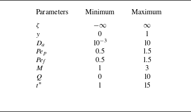
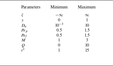
The selection of parameter values in this study is based on a comprehensive review of existing literature (Chen & Wu Reference Chen and Wu2012). Table 1 presents the range of parameter values used in these investigations. The Darcy number (
 $ D_a$
) indicates permeability, where a higher
 $ D_a$
signifies more permeable, less compact pore geometry, and a lower
 $ D_a$
signifies less permeable, more compact geometry. The viscosity ratio (
 $ M$
), representing the ratio of two viscosities, is crucial for exploring the impact on fluid dynamics. The pressure gradient (
 $ Q$
), expressed as
 $ -({{\rm d}p}/{{\rm d}x)}/({\mu U}/{H^2})$
, allows for the analysis of the influence on the composite region, with different
 $ Q$
values representing varying pressure gradients, facilitating the examination of flow behaviour under different pressure conditions. Finally, time (
 $ t^*$
) represents the temporal aspect of pollutant dispersion, enabling the analysis of how pollutant concentration and distribution evolve over time. The Péclet numbers (
 ${\textit{Pe}}_p$
and
 ${\textit{Pe}}_{\!f}$
) are dimensionless numbers that characterise the relative importance of advection to diffusion in the transport processes, with their values indicating the dominance of one mechanism over the other.
Range of parameter values.
4.2. Computational results and validations
The expression for the two-dimensional concentration distribution can be derived from (3.17) and (3.18) in the new coordinate system
 $\{\zeta ,y\}$
as
 \begin{equation} C=\begin{cases} C^{(0)}+\epsilon {\textit{Pe}}_{p}N_p(y)\dfrac {\partial C^{(0)}}{\partial \zeta }+\epsilon ^2{\textit{Pe}}_p X_p(y)\dfrac {\partial ^2 C^{(0)}}{\partial {\zeta }^2}, & 0\lt y\leqslant h,\\[10pt] C^{(0)}+\epsilon {\textit{Pe}}_{\!f}N_{\!f}(y)\dfrac {\partial C^{(0)}}{\partial \zeta }+\epsilon ^2{\textit{Pe}}_{\!f} X_{\!f}(y)\dfrac {\partial ^2 C^{(0)}}{\partial {\zeta }^2}, & h \leqslant y\lt 1. \end{cases} \end{equation}
We used the finite difference discretisation technique, as explained in Appendix D, to obtain the following discrete forms of (3.7) and (3.8) as follows:
 \begin{align} & {\textit{Pe}}_p \left \langle \frac {1}{\textit{Pe}} \right \rangle \frac {C_{p_{i,j}}^{n+1} - C_{p_{i,j}}^{n}}{\Delta t^*} \nonumber\\ & \quad + {\textit{Pe}}_p \left \{ {\text{max}} (u_p - \langle u \rangle , 0) \frac {C_{p_{i,j}}^{n} - C_{p_{i-1,j}}^{n}}{\Delta \zeta } - {\text{max}} (\langle u \rangle - u_p, 0) \frac {C_{p_{i+1,j}}^{n} - C_{p_{i,j}}^{n}}{\Delta \zeta } \right \} \nonumber\\ & = \frac {C_{p_{i+1,j}}^{n} - 2C_{p_{i,j}}^{n} + C_{p_{i-1,j}}^{n}}{\Delta \zeta ^2}+\frac {C_{p_{i,j+1}}^{n} - 2C_{p_{i,j}}^{n} + C_{p_{i,j-1}}^{n}}{\Delta y^2}, \quad j=0,1,\ldots ,j_h, \end{align}
 \begin{align} & {\textit{Pe}}_{\!f} \left \langle \frac {1}{\textit{Pe}} \right \rangle \frac {C_{f_{i,j}}^{n+1} - C_{f_{i,j}}^{n}}{\Delta t^*} \nonumber\\ & \quad + {\textit{Pe}}_{\!f} \left \{ {\text{max}} (u_p - \langle u \rangle , 0) \frac {C_{f_{i,j}}^{n} - C_{f_{i-1,j}}^{n}}{\Delta \zeta } - {\text{max}} (\langle u \rangle - u_{\!f}, 0) \frac {C_{f_{i+1,j}}^{n} - C_{f_{i,j}}^{n}}{\Delta \zeta } \right \} \nonumber\\ & = \frac {C_{f_{i+1,j}}^{n} - 2C_{f_{i,j}}^{n} + C_{f_{i-1,j}}^{n}}{\Delta \zeta ^2}+\frac {C_{f_{i,j+1}}^{n} - 2C_{f_{i,j}}^{n} + C_{f_{i,j-1}}^{n}}{\Delta y^2}, \quad j=j_h,j_h+1,\ldots N_y. \end{align}
Here
 $i=0,1,2,\ldots ,M_x$
and
 $j=0,1,2\ldots ,N_y$
;
 $M_x$
and
 $N_y$
represent the maximum number of grid points along the
 $\zeta$
and
 $y$
direction, respectively. The computational domain considered is
 $[-20,20]\times [0,1]$
. We discretise the domain using
 $2001$
grid points in the longitudinal direction and
 $101$
grid points in the transverse direction, corresponding to
 $\Delta x = L_x/(M_x-1)$
and
 $\Delta y = L_y/(N_y-1)$
. The time step is chosen as
 \begin{equation} \Delta t = \frac {0.4}{(1/\Delta x^2 + 1/\Delta y^2)}, \end{equation}
which satisfies the stability condition of the explicit scheme.
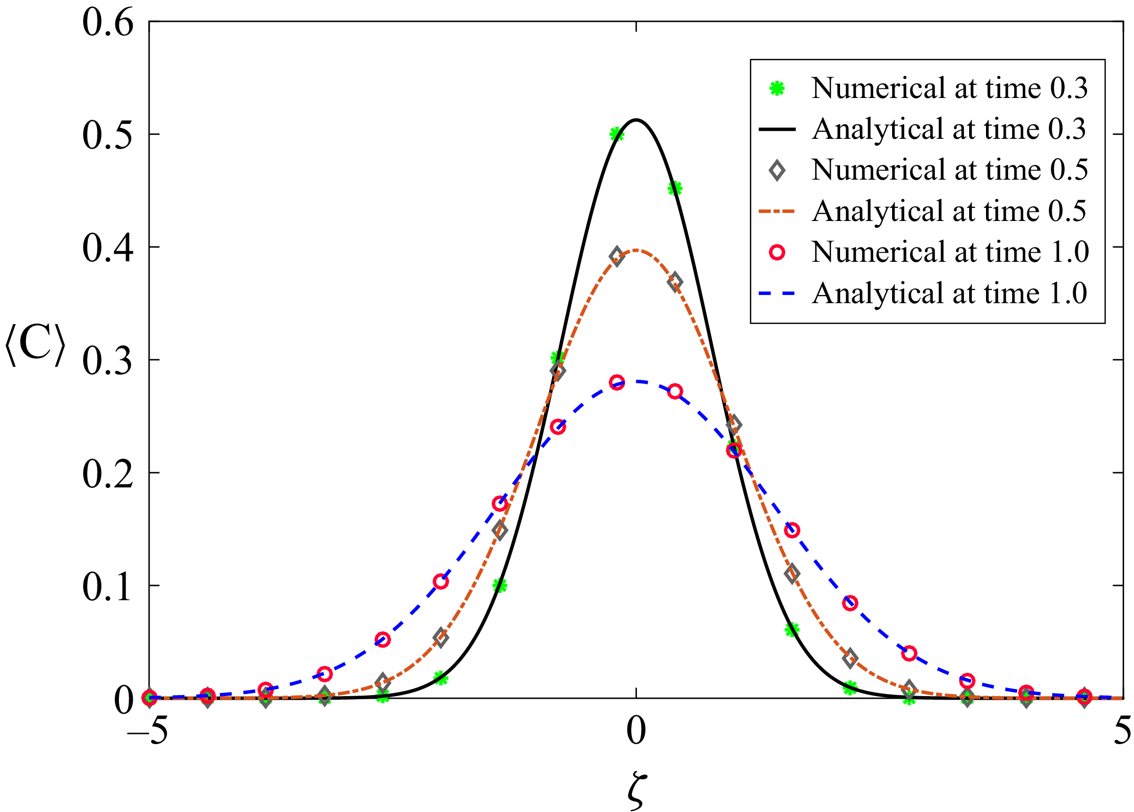
Comparison between analytical and numerical results of a two-dimensional concentration distribution for different times with
 $M=1$
,
 ${\textit{Pe}}_p={\textit{Pe}}_{\!f}=1$
,
 $Q=1$
,
 $h=0.5$
,
 $D_a=0.1$
.
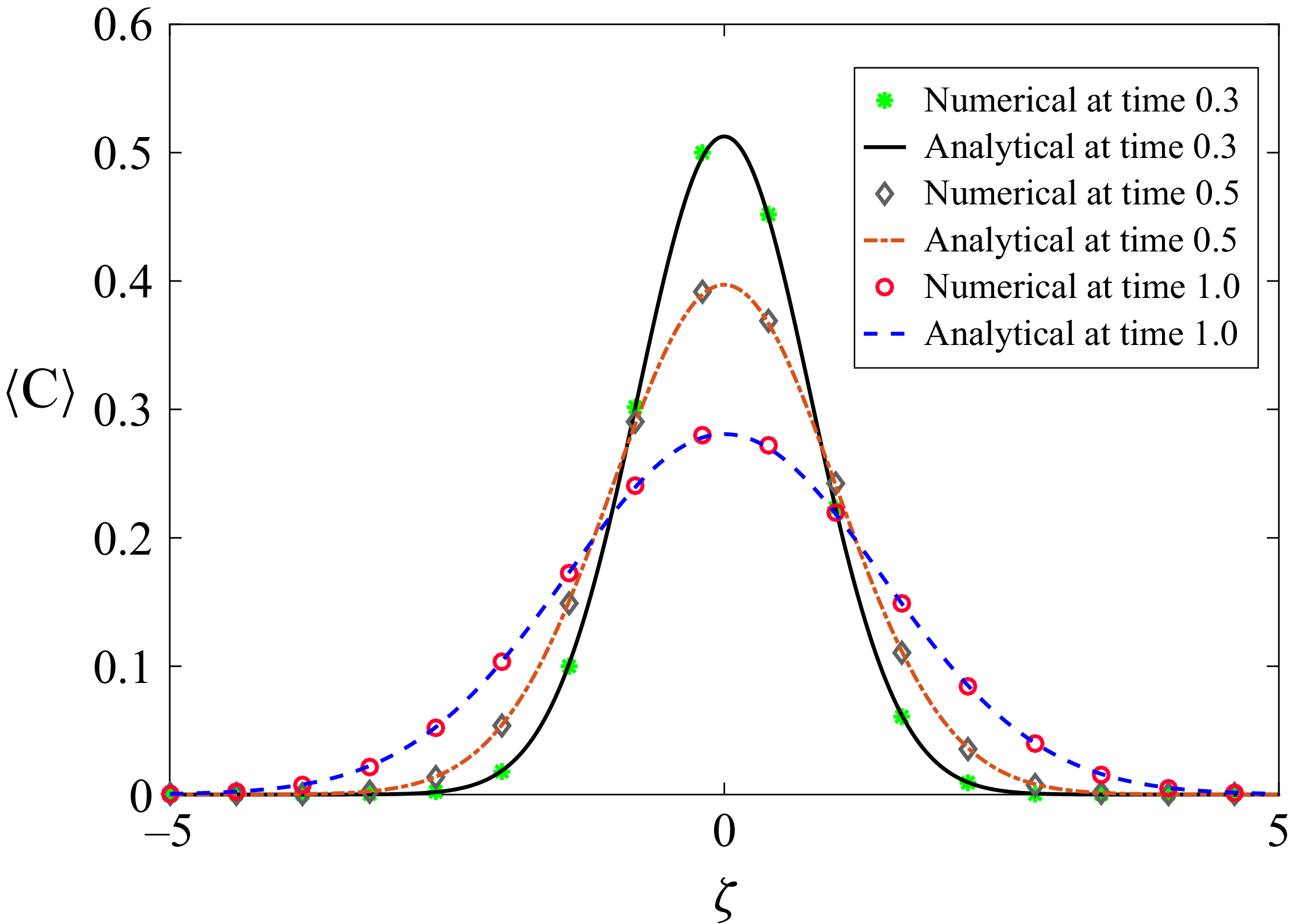
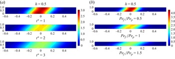
In figure 2 we present a comparative analysis between the analytical and numerical results over time. The graph shows a strong relation between the two-dimensional concentration distributions obtained from both the analytical and computational approaches. Although experimental data for this specific case is not available, we have provided a comparison with results derived from computational methods. This comparison highlights the consistency between the two methods and validates the reliability of the computational model in capturing the behaviour predicted by the analytical solution. Despite the absence of experimental verification, the close agreement between these solution methods reinforces the accuracy and applicability of both methods in predicting this phenomenon.
4.3. Dispersion coefficients
The effective dispersion coefficient can be expressed in (3.57) as
 \begin{equation} D_T = 1 + D_T^*. \end{equation}
The value of
 $D_T^*$
takes into account the impact of lateral diffusion and advection and is calculated as
 $-{\langle PeuN(y) \rangle }/{\langle {1}/{\textit{Pe}} \rangle }$
. On the right-hand side, the constant term of (4.5), i.e. the one representing the effect of longitudinal diffusion, can be safely ignored to focus on the enhanced effects of lateral diffusion and advection. The dispersion coefficient (
 $D_T^*$
) is influenced by various parameters such as
 ${\textit{Pe}}_{\!f}$
,
 ${\textit{Pe}}_p$
,
 $M$
,
 $h$
,
 $Q$
and
 $D_a$
. When the Darcy number(
 $D_a$
) is large,
 $D_T^*$
becomes 0.0083
 $Pe^2_{\!f}$
, which is the same as the finding of Barik & Dalal (Reference Barik and Dalal2018). This value represents the degree of dispersion of the solute in the fluid medium under single-zone open channel conditions (i.e.
 $h=0$
in our case).
Variation of dispersion for (a)
 $M=1, {\textit{Pe}}_p={\textit{Pe}}_{\!f}=1, Q=1$
and (b)
 $D_a=1, {\textit{Pe}}_p=1, M=1, Q=1$
.
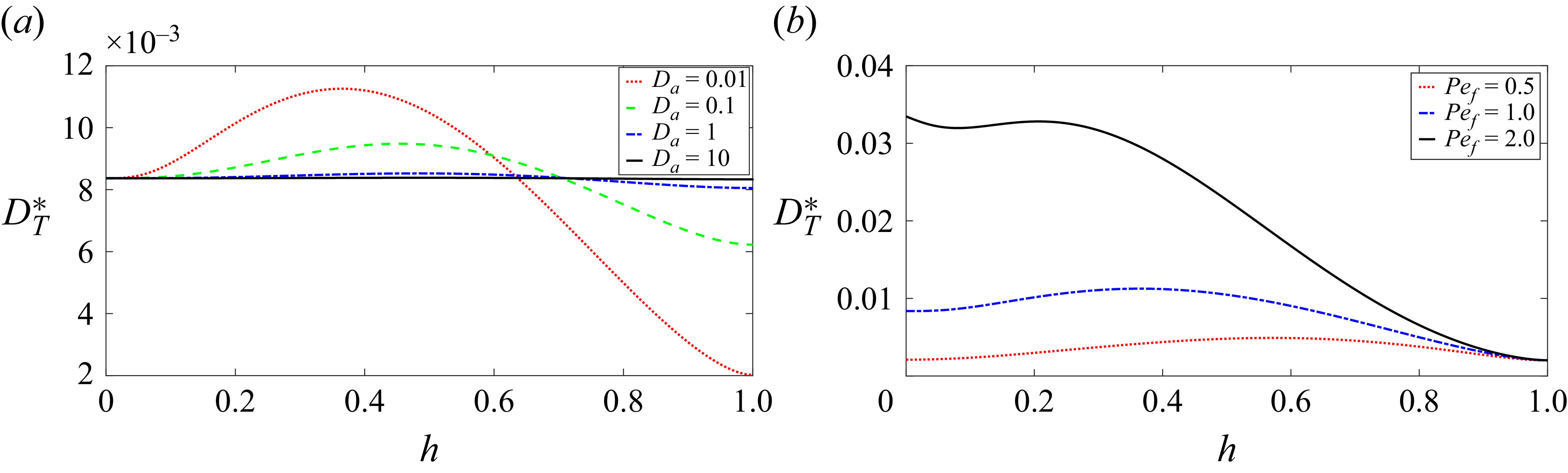
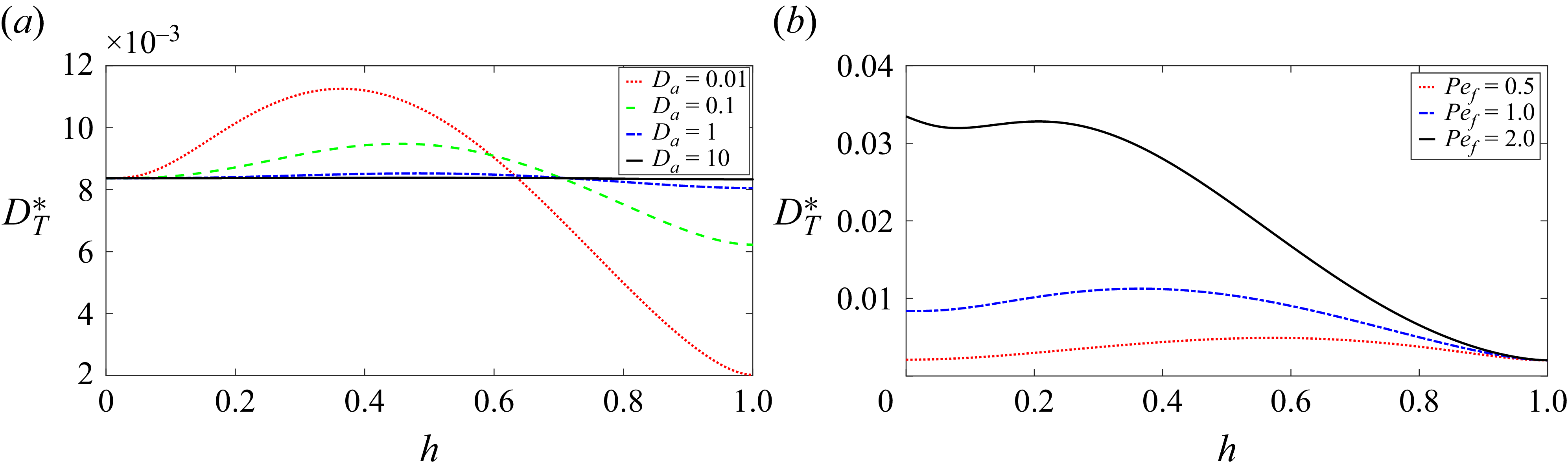
Figure 3(a) shows the variation of dispersion for different
 $D_a$
values. We can see from this that an increase in
 $D_a$
leads to decrease in the dispersion value and a flatter dispersion graph, which is same as in Chen & Wu (Reference Chen and Wu2012). When the value of
 $D_a$
is 0.01, the dispersion coefficient displays a discernible pattern. It gradually increases until it reaches a specific value of
 $h$
, which is not fixed for every
 $D_a$
, after which it experiences a rapid decrease. When
 $D_a$
is high, fluid flow through porous media becomes more efficient, and advection becomes increasingly essential compared with diffusion. When advection dominates (high
 $D_a$
), the dispersion graph becomes flatter because advection rapidly homogenises the solute concentration within the porous medium. The variation of dispersion graphs with different Péclet numbers for the fluid phase (
 ${\textit{Pe}}_{\!f}$
), as depicted in figure 3(b), illustrates a clear relationship between
 ${\textit{Pe}}_{\!f}$
values and the dispersion coefficient. As
 ${\textit{Pe}}_{\!f}$
increases, it can be noticed that the dispersion coefficient also increases (Chen & Wu Reference Chen and Wu2012).
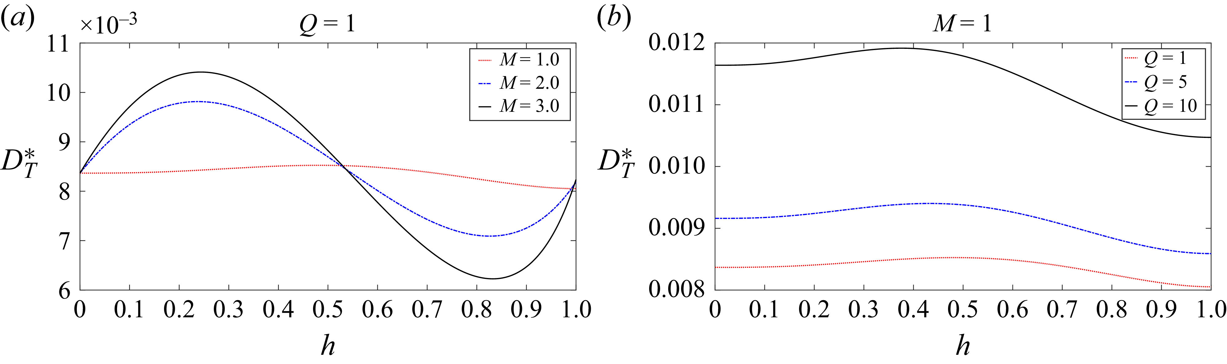
Figure 4(a) illustrates the variation of dispersion coefficient with respect to the height of the porous region,
 $h$
, for different values of
 $M$
, which represents the ratio of effective viscosity to the dynamic viscosity. For each value of
 $M$
, the dispersion initially increases as
 $h$
increases from 0 to 0.3, and then shows varying behaviour for higher
 $h$
. When
 $h=0.5$
, the dispersion remains relatively stable or slightly decreases, but for higher values of
 $h$
(around 0.8 and 1), we observe a general decline in dispersion. The height of the porous region,
 $h$
, affects the flow dynamics and the spread of particles within the porous medium. At lower heights (
 $h = 0$
to
 $h = 0.3$
), the flow is less constrained because the porous region is not fully developed, leading to weaker interactions between the fluid and porous medium. As a result, the dispersion initially increases due to less resistance and more mobility of fluid particles. However, as
 $h$
increases, the porous medium becomes more dominant, imposing greater resistance to flow, which in turn slows down the dispersion. This leads to a peak or plateau in dispersion values around
 $h = 0.3$
, followed by a decline as the resistance further increases with larger
 $h$
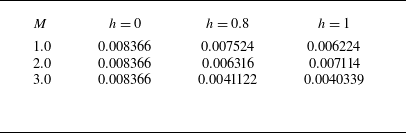
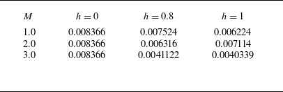
. This phenomenon can be seen in the values displayed in table 2.
Values of
 $D_T^*$
for different values of
 $M$
and
 $h$
.
Variation of dispersion for (a)
 $ {\textit{Pe}}_p={\textit{Pe}}_{\!f}=1, Q=1$
and
 $D_a=1$
, and (b)
 $ {\textit{Pe}}_p={\textit{Pe}}_{\!f}=1, M=1$
and
 $D_a=1$
.
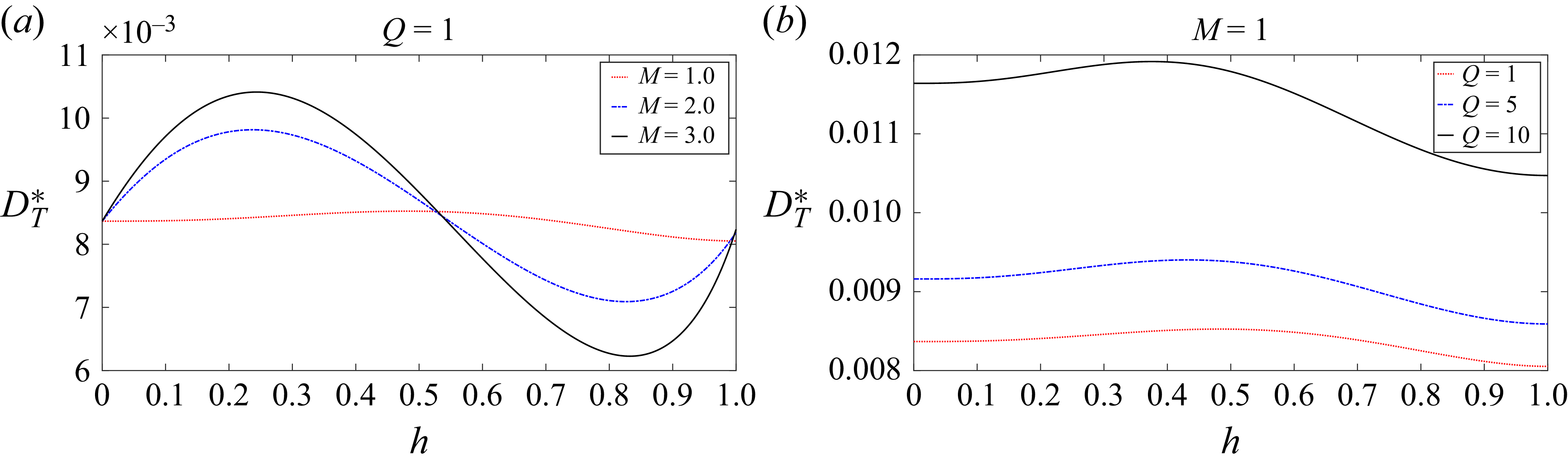
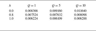
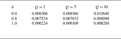
Table 3 and figure 4(b) present the variations in dispersion coefficient (
 $D_T^*$
) as influenced by the height (
 $ h$
) of the porous region and the pressure gradient (
 $ Q$
). With a constant pressure gradient, the dispersion coefficient increases with the increase in the height of the porous region, and with a fixed height of the porous medium, the dispersion coefficient increases as the pressure gradient increases.
Dispersion (
 $D_T^*$
) values at various heights (
 $h$
) for different pressure gradients (
 $Q$
).
4.4. Mean concentration
The mean concentration distribution can be computed using (3.17), (3.18) and (3.72) as
 \begin{equation} \langle C\rangle =C^{(0)} = \frac {1}{\sqrt { 4\pi D_T t^*}}\exp \left (\frac {-\zeta ^2}{4 D_T t^*}\right )\!. \end{equation}
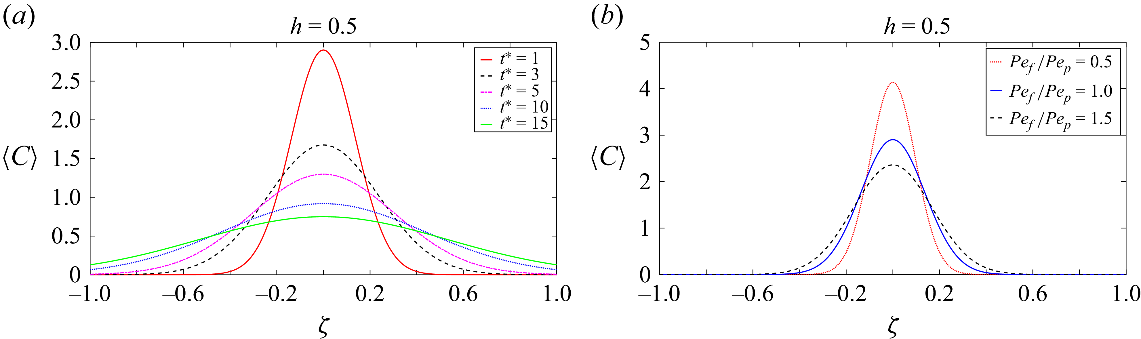
Longitudinal distribution of mean concentration distributions for different values of (a) time, where
 $M=1$
,
 ${\textit{Pe}}_p={\textit{Pe}}_{\!f}=1$
,
 $Q=1$
,
 $D_a=0.1$
and (b) Péclet numbers ratio, where
 $t^*=1$
,
 $Q=1$
,
 $M=1$
,
 $D_a=0.1$
.
Longitudinal distribution of mean concentration distributions for
 $M=1,{\textit{Pe}}_P={\textit{Pe}}_{\!f}=1,Q=1$
and
 $t^*=1$
.
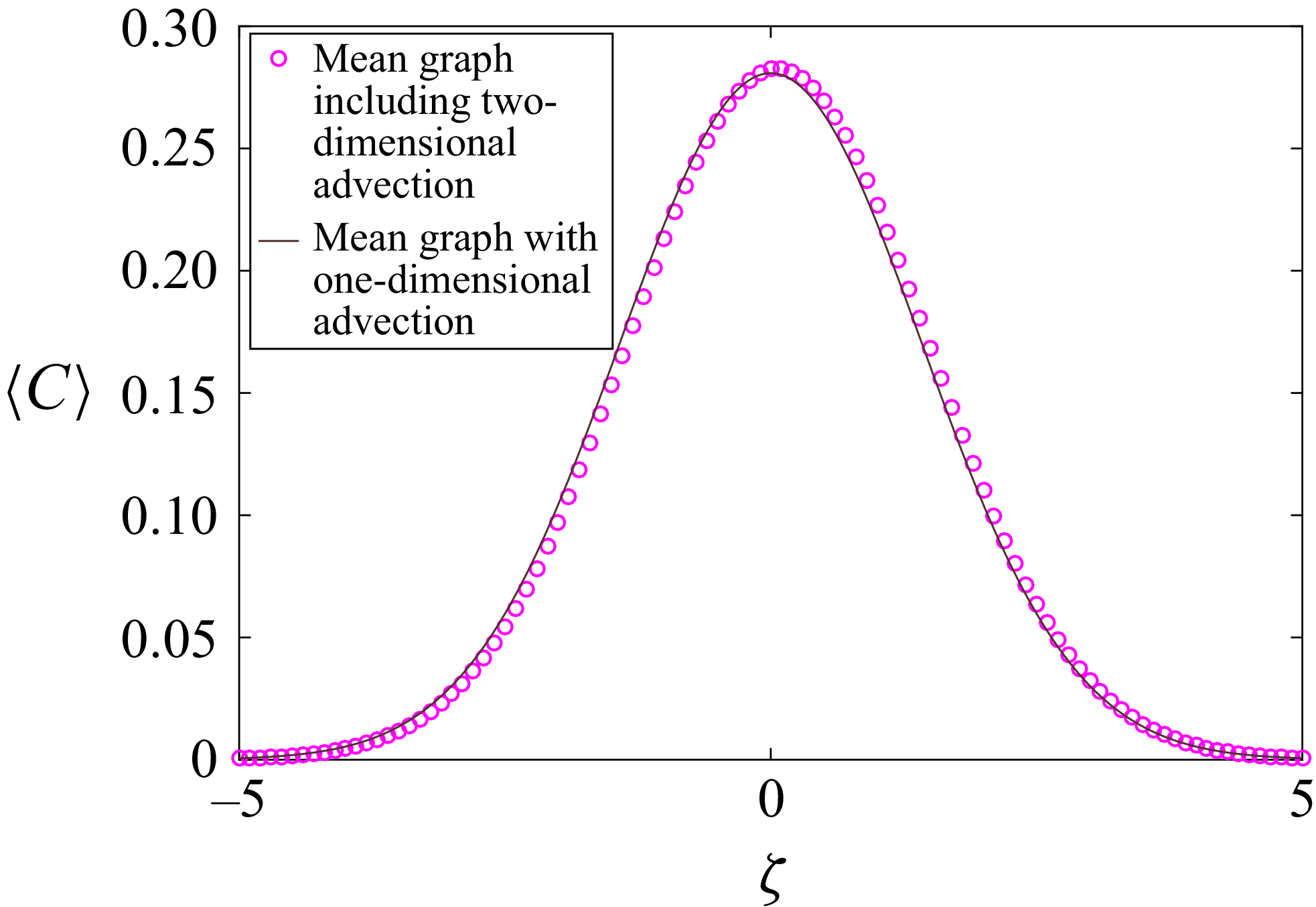
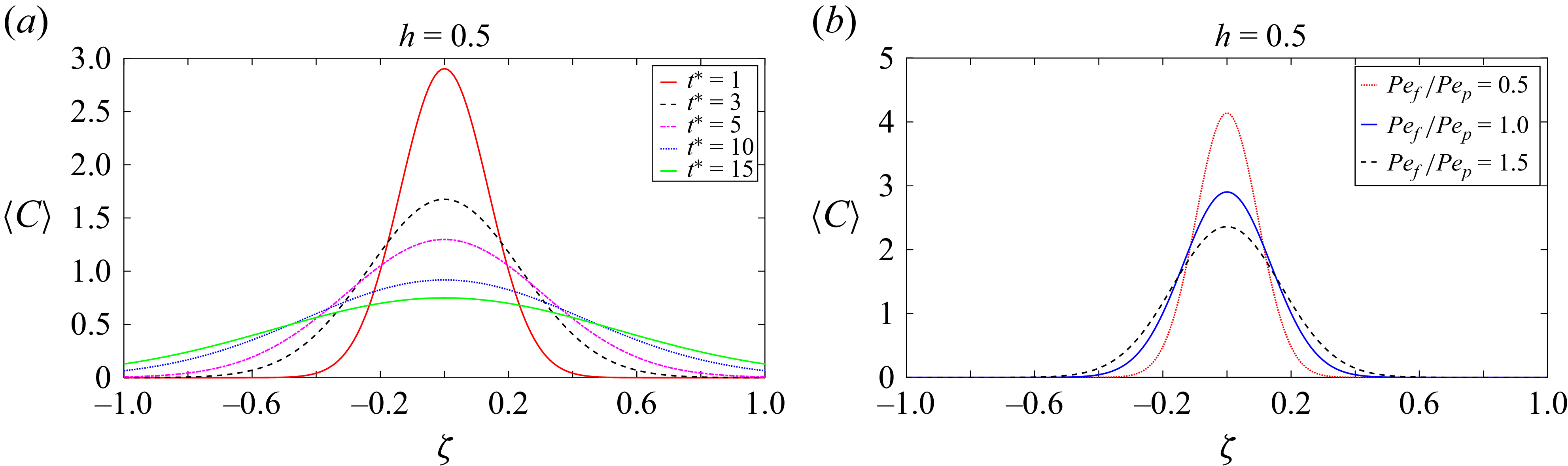
The variations of the longitudinal distribution of mean concentration can be seen from figures 5, 6 and 7. Figure 5(a) displays the change in the mean concentration distribution with time. At a fixed time, the mean concentration exhibits a Gaussian distribution, which is characterised by its symmetrical shape and adherence to statistical normality. The axis of symmetry remains unchanged, therefore partitioning the distribution into two symmetrical components. Over time, the apex of the distribution progressively decreases and becomes flatter.
The graph in figure 5(b) demonstrates how the ratio of the Péclet numbers
 $({\textit{Pe}}_{\!f}/{\textit{Pe}}_p)$
affects the mean concentration at a specific height
 $(h = 0.5)$
. When
 $({\textit{Pe}}_{\!f}/{\textit{Pe}}_p)$
increases, the Péclet number of the fluid phase
 $({\textit{Pe}}_{\!f})$
becomes higher than that of the porous phase
 $({\textit{Pe}}_p)$
, resulting in a decrease in the peak of the mean concentration graph. This occurs because advection in the fluid phase becomes more influential, resulting into better transport of solutes. As a result, the solutes are more effectively carried away from the peak concentration point, causing a lower peak.
Longitudinal distribution of mean concentration distributions for
 $M=1,{\textit{Pe}}_p={\textit{Pe}}_{\!f}=1,h=0.5,D_a=0.1$
and
 $t^*=1$
.
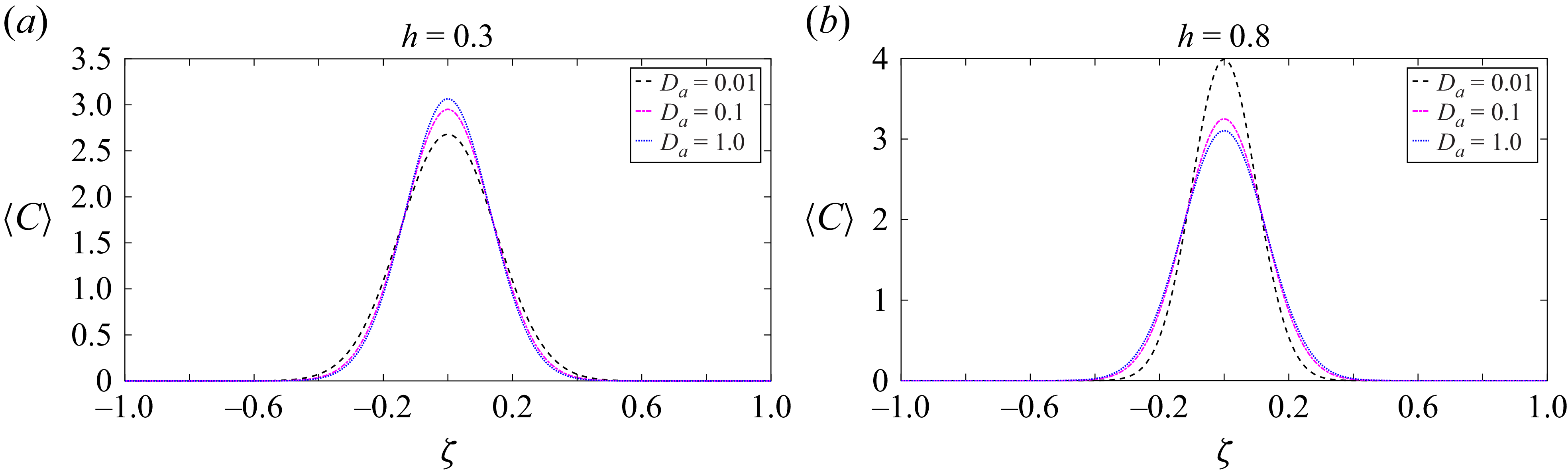
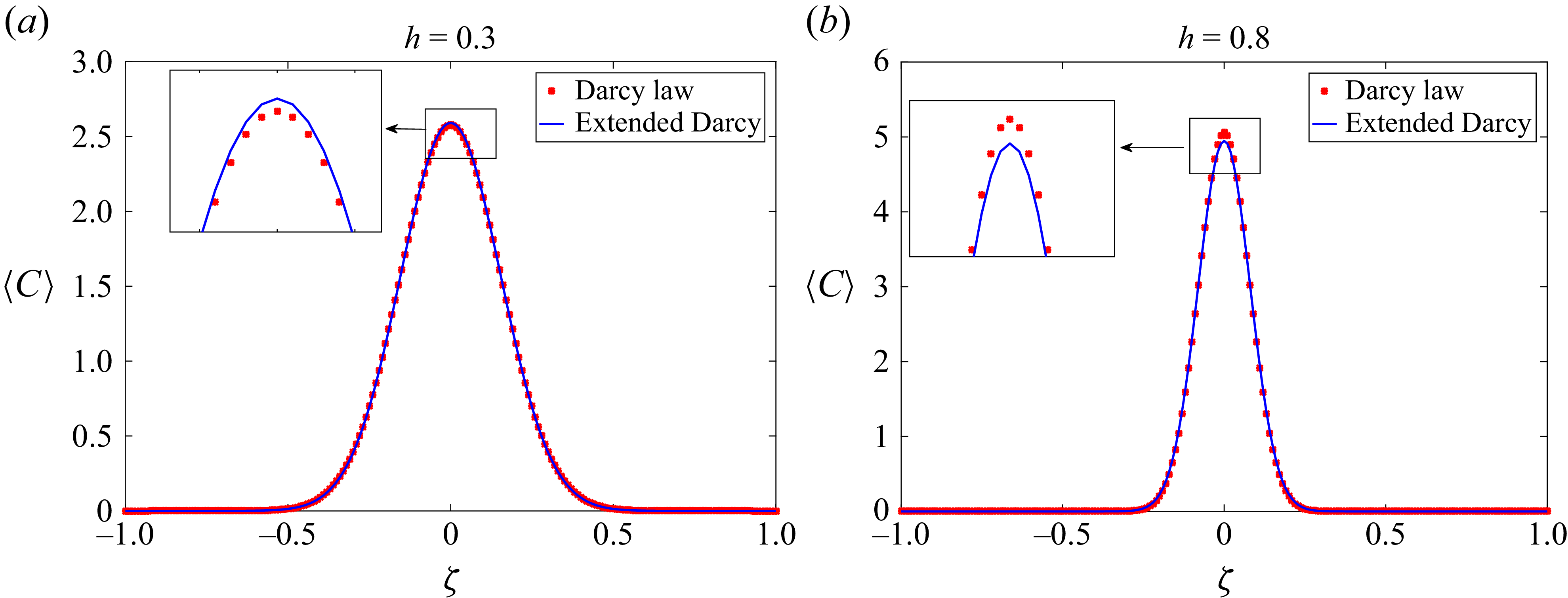
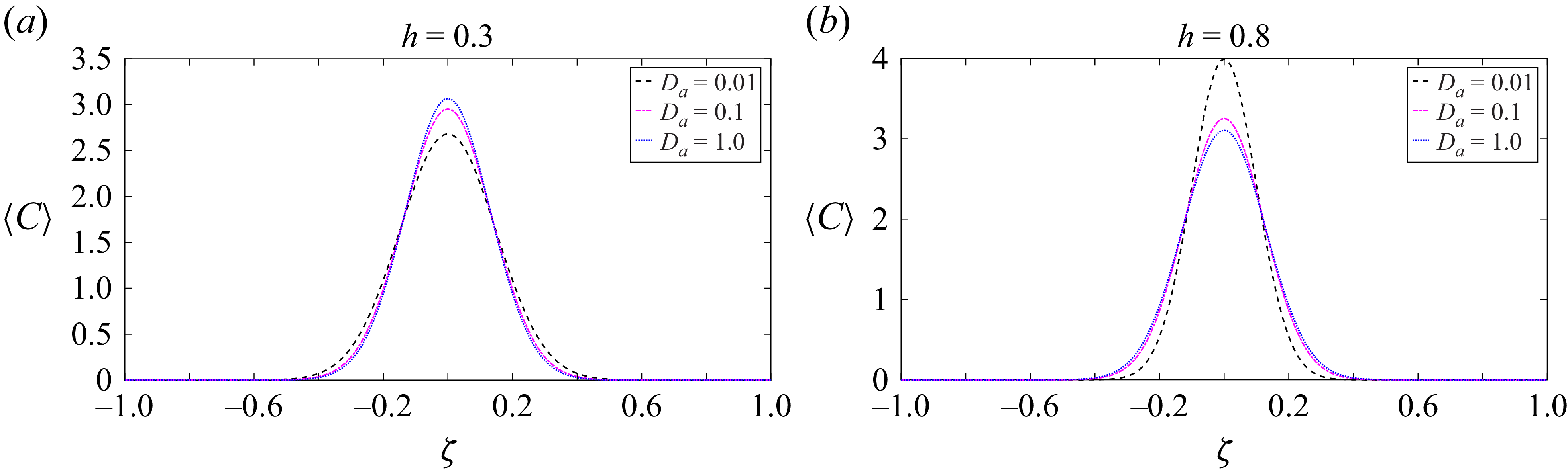
Figures 6(a) and 6(b) show that the mean concentration distribution undergoes significant changes with the Darcy number
 $(D_a)$
in a two-layered channel flow. It is worth noting that these trends correlate with the behaviour of the dispersion coefficient, as demonstrated in figure 3. In figure 3(a) for
 $h = 0.3$
, we can see that dispersion increases with a lower Darcy number, causing the peak of the mean concentration to decrease, as shown in figure 6(a). This happens because as
 $D_a$
goes down, the effect of molecular diffusion on dispersion becomes stronger. This makes solutes spread out more and lowers their peak concentrations. Conversely, for
 $h = 0.8$
, a lower
 $D_a$
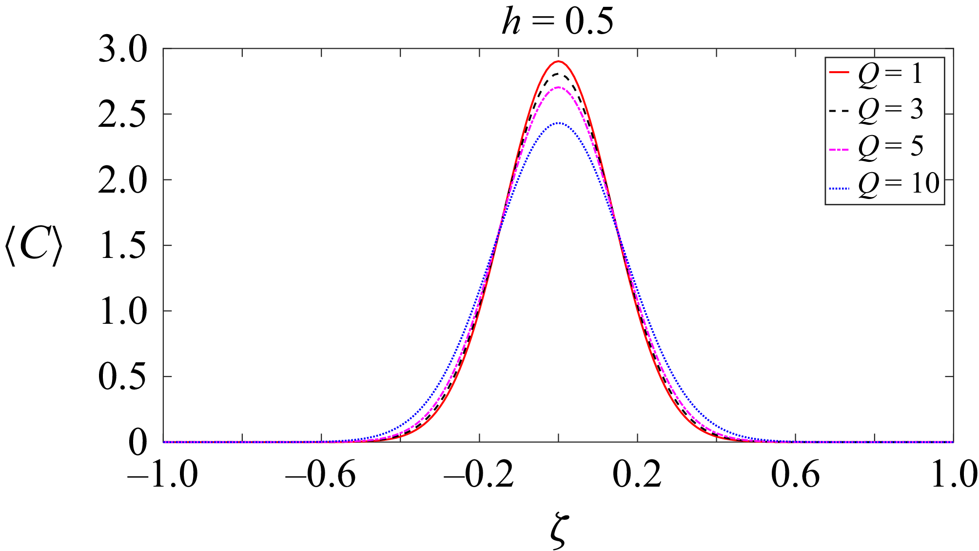
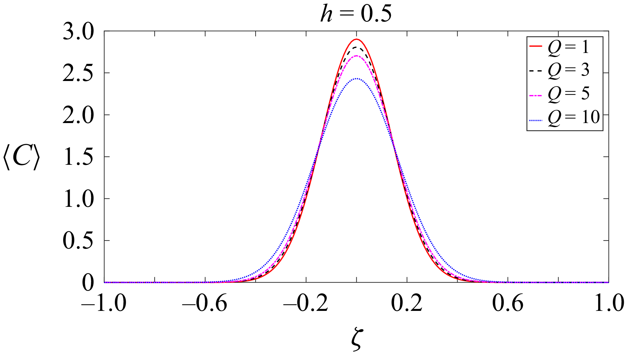
corresponds to decreased dispersion, resulting in an increased peak of the mean concentration, as illustrated in figure 6(b). In this case, advection is more prominent in the channel, carrying solutes away more quickly and thus reducing peak concentrations. Figure 7 displays the distribution of mean concentration for different
 $Q$
values while keeping the parameters constant at
 $h = 0.5$
. Our observation indicates that lower
 $Q$
values result in a higher concentration peak, thus leading to greater solute spreading when the
 $Q$
value is high. This finding is consistent with the dispersion graph presented in figure 4(b).
4.5. Longitudinal concentration distribution
The expression for the two-dimensional concentration distribution up to second order can be derived from (3.17) and (3.18) in the new coordinate system
 $\{\zeta ,y\}$
as
 \begin{equation} C=\begin{cases} C^{(0)}+\epsilon {\textit{Pe}}_{p}N_p(y)\dfrac {\partial C^{(0)}}{\partial \zeta }+\epsilon ^2{\textit{Pe}}_p X_p(y)\dfrac {\partial ^2 C^{(0)}}{\partial {\zeta }^2}, & 0\lt y\leqslant h,\\[8pt] C^{(0)}+\epsilon {\textit{Pe}}_{\!f}N_{\!f}(y)\dfrac {\partial C^{(0)}}{\partial \zeta }+\epsilon ^2{\textit{Pe}}_{\!f} X_{\!f}(y)\dfrac {\partial ^2 C^{(0)}}{\partial {\zeta }^2}, & h \leqslant y\lt 1. \end{cases} \end{equation}
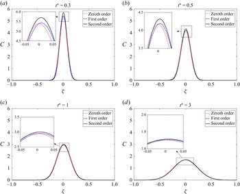
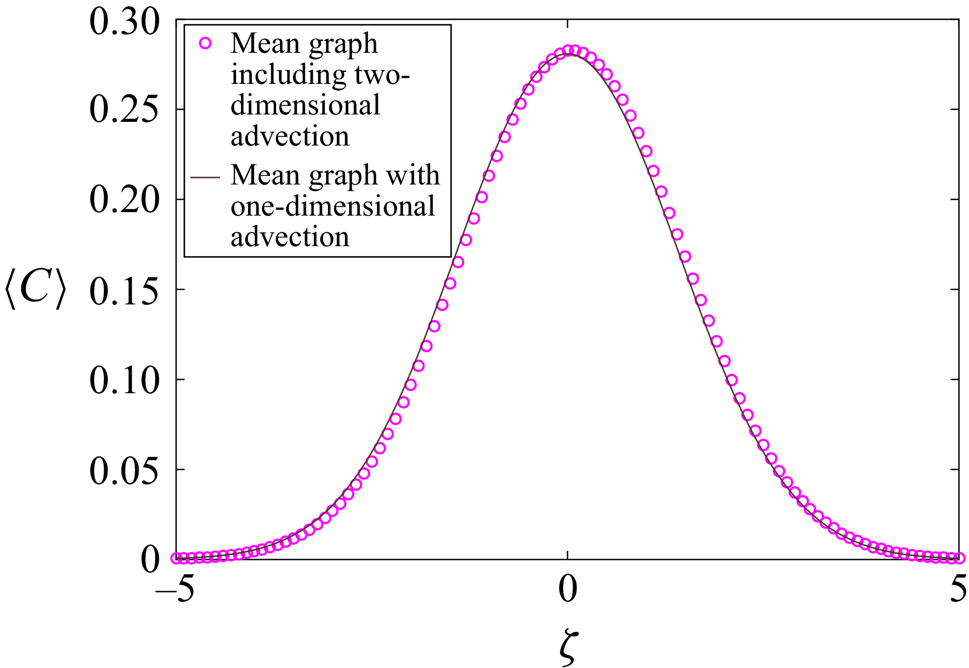
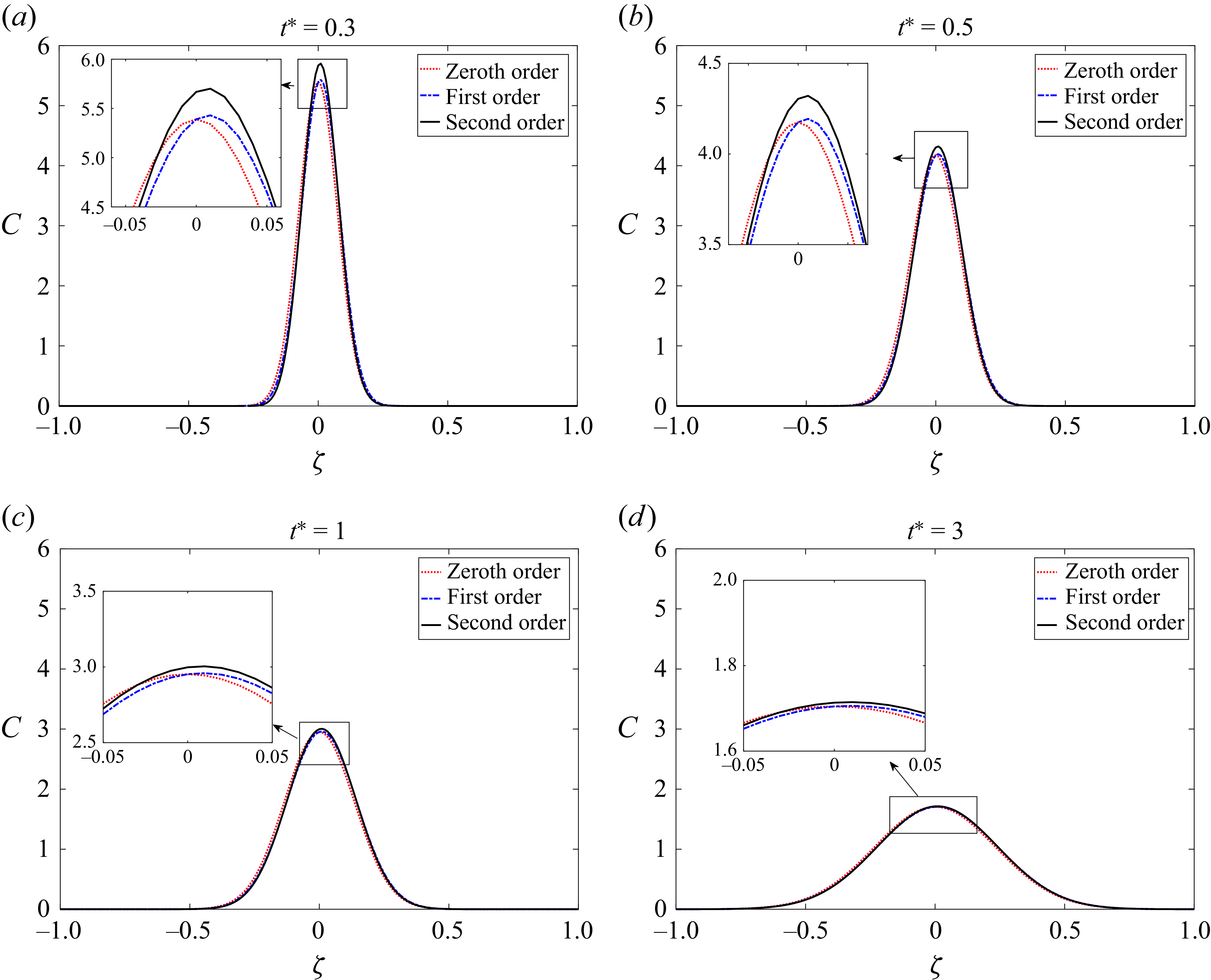
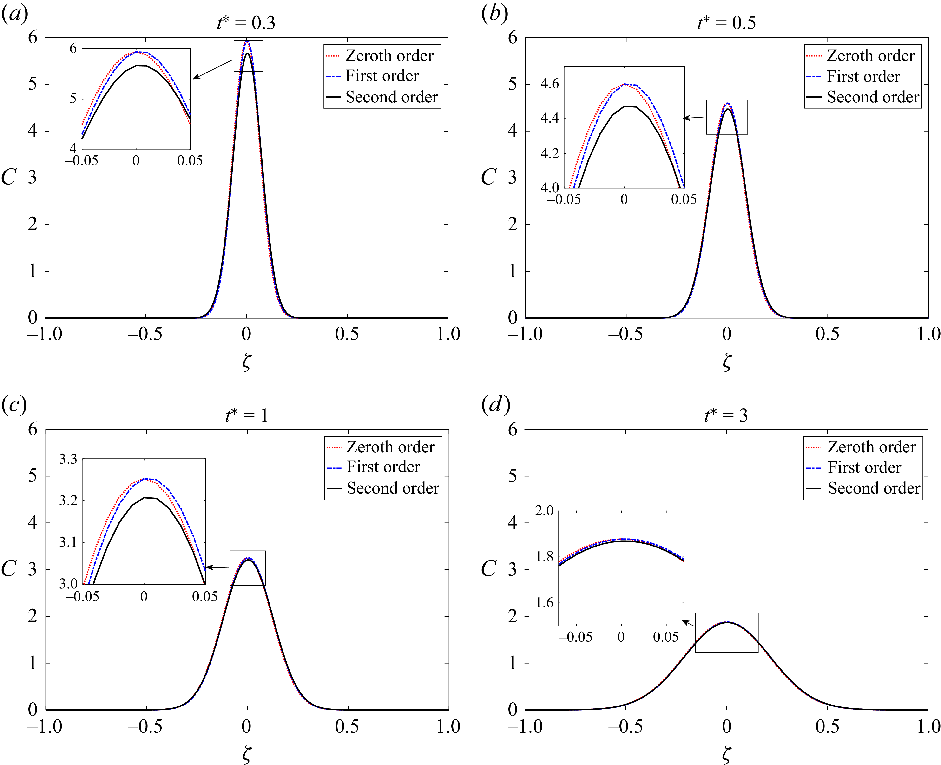
Figures 8 and 9 show the longitudinal solute distribution along the channel, illustrating the gradual transition from zeroth order to second order at different times. Initially, for
 $t^* \lt 1$
, the contributions of each order term are significant in shaping the solute concentration along the channel. However, as time progresses, the influence of higher-order terms diminishes. After
 $t^* = 1$
, neglecting terms beyond the second order introduces minimal error, as indicated by figures 8 and 9. As a result, the graphs for zeroth-order, first-order and second-order approximations become nearly indistinguishable for a considerable period when
 $t^* \gt 1$
.
Longitudinal distribution of concentration calculated as asymptotic expansions from zeroth order to second order at different times, where
 $M=1$
,
 ${\textit{Pe}}_p={\textit{Pe}}_{\!f}=1$
,
 $h=0.3$
,
 $Q=1$
,
 $y=0.5$
,
 $D_a=0.1$
.
Longitudinal distribution of concentration calculated as asymptotic expansions from zeroth order to second order at different times, where
 $M=1$
,
 ${\textit{Pe}}_p={\textit{Pe}}_{\!f}=1$
,
 $h=0.8$
,
 $Q=1$
,
 $y=0.5$
,
 $D_a=0.1$
.
Concentration contour: the horizontal coordinate represents the variable
 $\zeta$
, while the vertical coordinate represents the variable
 $y$
for different values of time (
 $t^*$
) and
 ${{\textit{Pe}}_{\!f}}/{{\textit{Pe}}_p}$
where (a)
 $M=1, Q=1, D_a=0.1, {\textit{Pe}}_p={\textit{Pe}}_{\!f}=1$
and (b)
 $M=1, D_a=0.1, t^*=1, Q=1$
.
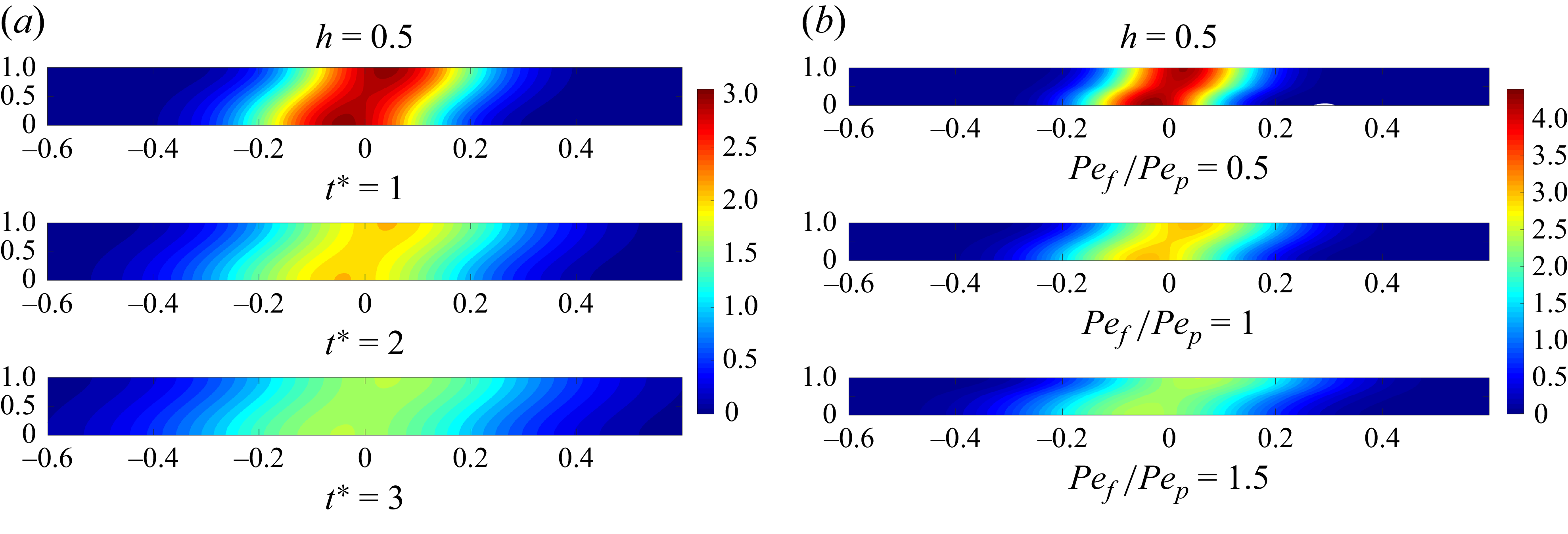
Figures 10 and 11 display the concentration contours for different values of the parameters. Figure 10(a) presents the solute spreading dynamics over time in the two-layered channel system. Here, we plot the contour graphs for the porous region, which spans from 0 to 0.5 and the fluid region from 0.5 to 1. Initially, the solute is injected across the line
 $\zeta =0$
, the solute spreads due to advection and diffusion. The solute concentration experiences differential transport rates in the two regions: it travels faster in the fluid region compared with the porous area. This difference in transport velocities is primarily due to the higher permeability and reduced resistance to flow in the fluid region, allowing solute molecules to move more freely. As time progresses, the concentration centroid experiences a reduction in its value, indicating the spreading of the solute throughout the channel. This phenomenon arises from advection, which propels solute downstream, and diffusion, which causes dispersion by random molecular motion, ultimately leading to a broader solute concentration distribution.
In figure 10(b) the observation of a ratio between two Péclet numbers (
 ${{\textit{Pe}}_p}/{{\textit{Pe}}_{\!f}}$
) equals 0.5, resulting in the concentration cloud being at the origin near the bottom plate and near the upper plate along the
 $y$
axis. As the ratio of these Péclet numbers increases, solute dispersion becomes more pronounced. Furthermore, the observation that the solute cloud spreads more in the fluid region than in the porous region suggests that the fluid layer is more efficient in transporting solutes over long distances due to higher advection effects. These trends align with the behaviour of the dispersion coefficient, which is influenced by the relative contributions of advection and diffusion in the two regions, impacting the overall spread of the solute cloud.
Concentration contours: the horizontal coordinate represents
 $\zeta$
, while the vertical coordinate represents
 $y$
for different values of
 $D_a$
where (a)
 $M=1, Q=1, {\textit{Pe}}_p={\textit{Pe}}_{\!f}=1, h=0.3$
and (b)
 $M=1, Q=1, {\textit{Pe}}_p={\textit{Pe}}_{\!f}=1, h=0.8$
.
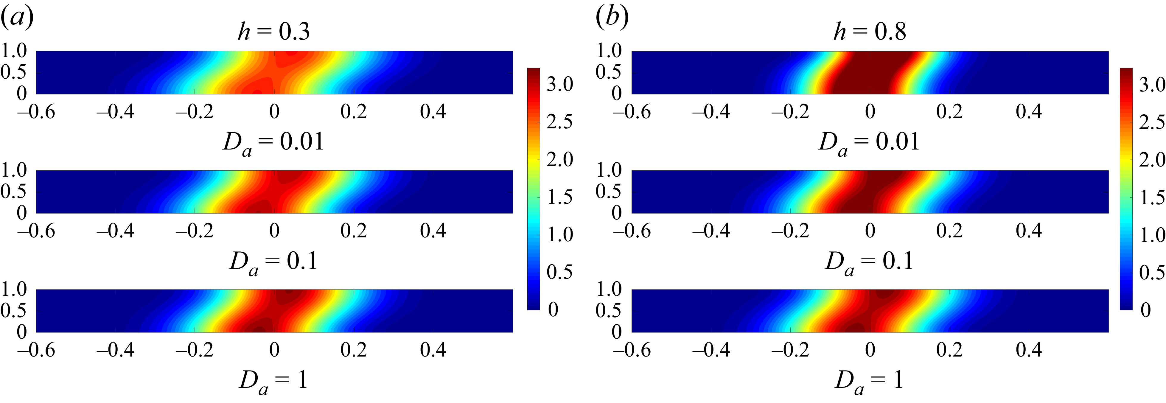
The observations in figures 11(a) and 11(b) provide valuable information into the behaviour of solute concentration distribution in a two-layered channel flow with differing heights (
 $h = 0.3$
and
 $h = 0.8$
). In figure 11(a) at
 $h = 0.3$
, it is clear that with decreasing Darcy number, solute spreads more. In contrast, at
 $h = 0.8$
(figure 11
b), the opposite trend is observed, an increase in the Darcy number results in more solute spreading. These observations align with the behaviour of the dispersion coefficient, as a lower Darcy number increases dispersion at
 $h = 0.3$
, while a higher Darcy number does so at
 $h = 0.8$
. The consistency between the dispersion and mean concentration results underline the interplay between advection and diffusion in influencing solute transport characteristics in two-layered channel flows with different heights.
4.6. Application of classical Darcy model in porous region
So far we were carrying out our investigations based on the extended Darcy equation (for the flow in porous media). However, based on one of the reviewers’ suggestions, we have now carried out the studies based on pure Darcy equations for the flow with low Darcy numbers and the extended Darcy equation for the flows with greater than those Darcy numbers. Fluid flow through porous media has been characterised using the empirical relationship known as Darcy’s law, i.e.
 \begin{equation} -\dfrac {{\rm d}p}{{\rm d}x'}-\mu \dfrac {u^{\prime}_{\!p}(y')}{\kappa }=0, \quad 0 \leqslant y'\leqslant h', \end{equation}
and the fluid motion in the fluid region (which is the same as (2.2))
 \begin{equation} - \dfrac {{\rm d}p}{{\rm d}x'} +\mu \dfrac {{\rm d}^2u^{\prime}_{\!f}}{{\rm d}y'^2} = 0,\quad h' \leqslant y' \leqslant H. \end{equation}
The initial and boundary conditions are
 \begin{align}&\qquad u^{\prime}_{\!p}(y')=u'_b \quad \text{at} \,y'=h', \end{align}
 \begin{align}& \dfrac {{\rm d}u^{\prime}_{\!f}(y')}{{\rm d}y'}=\beta '(u'_b-u^{\prime}_{\!p}) \quad \text{at}\,y'=h'. \end{align}
Dispersion graph of porous media using Darcy’s law for (a) different
 $Q$
and (b) different
 ${\textit{Pe}}_{\!f}$
.

Longitudinal distribution of mean concentration distributions for different values of (a)
 $h=0.3$
,
 $t^*=1$
,
 $D_a=0.001$
,
 $Q=1$
,
 $M=1$
and (b)
 $h=0.8$
,
 $t^*=1$
,
 $D_a=0.001$
,
 $Q=1$
,
 $M=1$
.
Here also
 $U$
is the flow velocity of the free surface:
 \begin{equation} u^{\prime}_{\!f}(y')= U \quad \text{at}\, y'=H. \end{equation}
Solving non-dimensional equations, we get the velocity components in the fluid and porous region, respectively, as
 \begin{align}& u_{\!f}=-Q\frac {y^2}{2}+ (Qh+\beta (u_b-u_p) )y+\left (1+\frac {Q}{2}-Qh-\beta (u_b-u_p)\right )\!, \end{align}
 \begin{align}&\qquad\qquad\qquad\qquad\qquad\qquad u_p=\textit{QD}_a, \end{align}
 \begin{align}&\qquad\qquad\quad u_b=\frac {Q\dfrac {h^2}{2}-Qh+1+\dfrac {Q}{2}-(h-1)\beta {\textit{QD}}_a}{1-(h-1)\beta }, \end{align}
where
 $u_b$
is the slip velocity and
 $\beta =({\alpha }/{\sqrt {\kappa }})$
is a parameter that depends on permeable surface properties;
 $\alpha$
is a dimensionless parameter that contains structural characteristic of the porous media known as the slip coefficient, defined as
 $\alpha =\sqrt {({\mu }/{\mu _e})}.$
Longitudinal distribution of mean concentration distributions for different values of (a)
 $h=0.3$
,
 $t^*=1$
,
 $D_a=0.1$
,
 $Q=1$
,
 $M=1$
and (b)
 $h=0.1$
,
 $t^*=1$
,
 $D_a=0.001$
,
 $Q=1$
,
 $M=1$
.
Darcy versus extended Darcy, where
 $h=0.3$
,
 $M=1.05$
,
 $Q=1$
,
 $t^*=1$
.
After obtaining the velocity profile, the multi-scale method is applied to determine the effective dispersion coefficient
 $ D^*_T$
and the mean concentration distribution
 $\langle C \rangle$
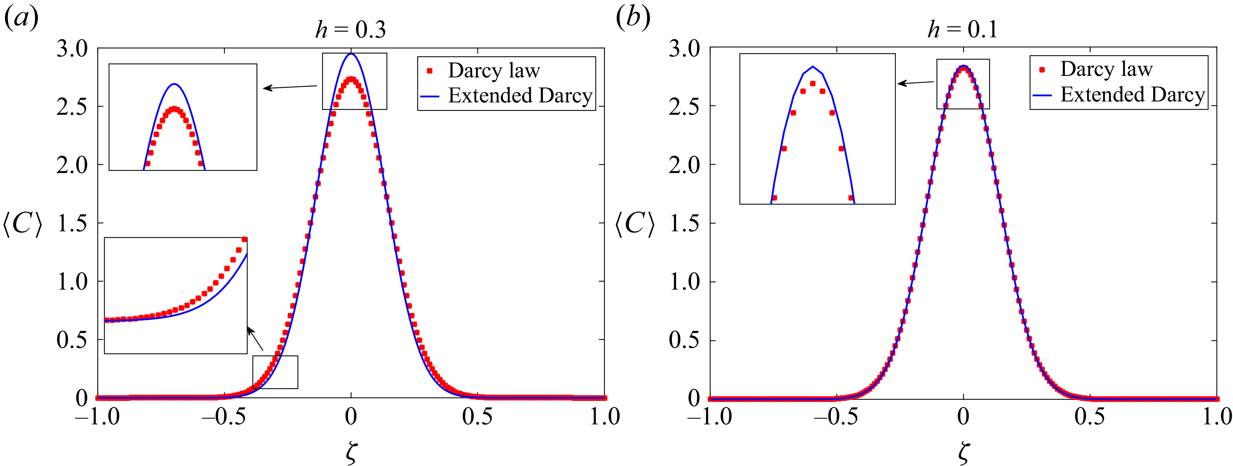
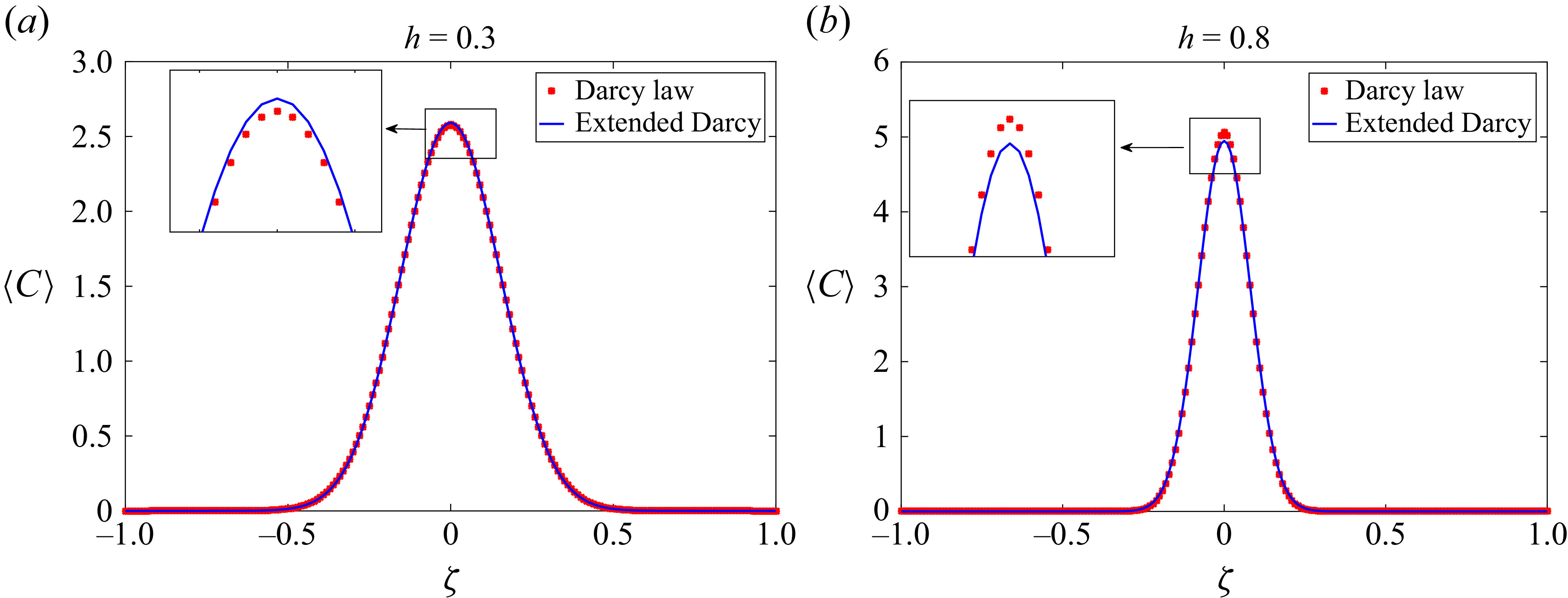
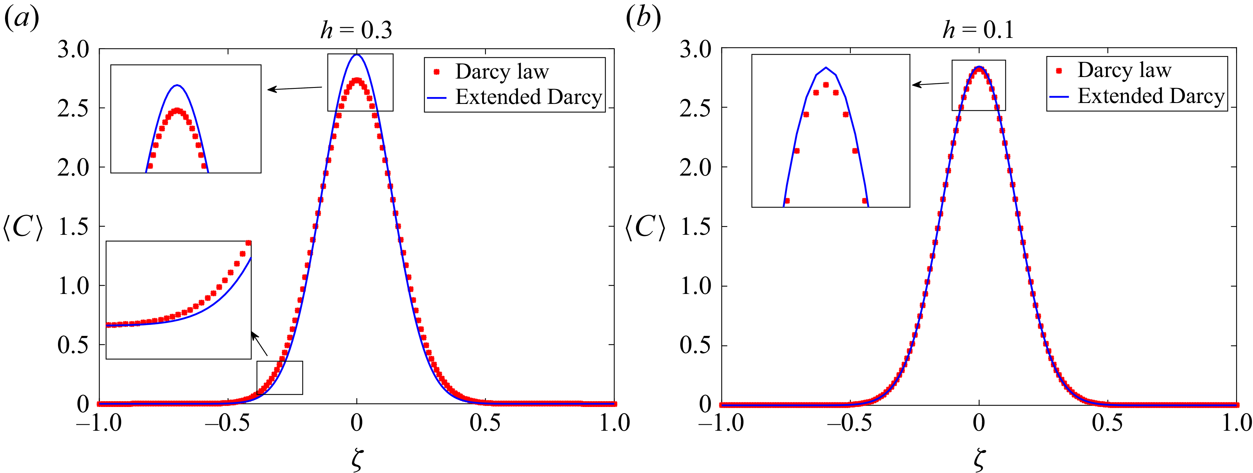
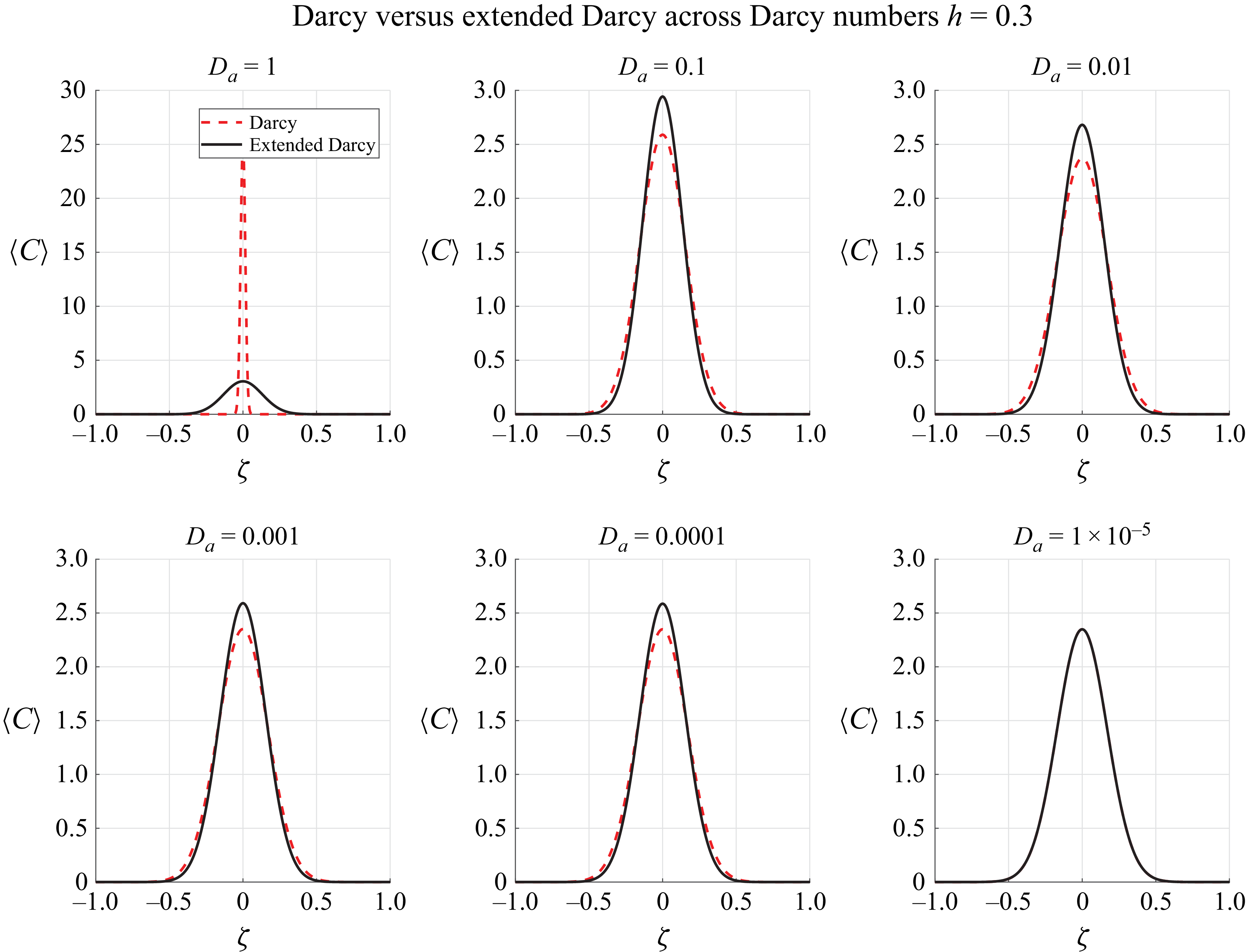
. Figures 13 and 14 indicate that when the height
 $( h )$
is small and permeability is low, the classical Darcy model and the extended Darcy model yield coinciding results. However, as
 $( h )$
increases or permeability becomes significant, noticeable differences between the two models emerge. From this observation, we can conclude that in cases where the porous medium is very thin and exhibits high permeability, the classical Darcy model is appropriate. Conversely, in scenarios where the porous region is relatively thicker and the permeability is not significantly high, the extended Darcy model (Brinkman model) should be employed for more accurate predictions, supporting the results of Winter et al. (Reference Winter, Valsamidou, Class and Flemisch2022). We present a detailed comparison between the classical Darcy law and the extended Darcy (Brinkman) model by varying the channel thickness parameter
 $h$
(considered at values
 $h = 0.3, 0.5, 0.8$
) and the viscosity ratio
 $M$
(taken as
 $M = 1$
and
 $M = 1.05$
). For the case
 $M = 1$
with permeability
 $\kappa = 10^{-5}$
, the difference between the Darcy and Brinkman models is not clearly visible (figure 13
b). To highlight the distinction more effectively, we next consider the case
 $M = 1.05$
with
 $\kappa = 0.1$
(figure 15). For
 $D_a = 1$
, the predictions of the extended Darcy (Brinkman) model differ markedly from the classical Darcy model, even for thin porous layers (
 $h = 0.3$
). This is because the viscous penetration length is
 $\mathcal{O}(H)$
, allowing interface shear to penetrate through the entire porous region. The classical Darcy model, lacking this shear-diffusion term, overconfines solute near the core. This aligns with studies showing that the Brinkman term becomes increasingly significant at higher permeability and across boundaries. For
 $D_a = 0.1$
and
 $0.01$
, the difference between the two models remains clear. The Brinkman solution continues to exhibit a smoother gradient at the interface and a broader profile. Here, the viscous penetration length
 $\ell _v$
is smaller but still larger than the porous thickness
 $h$
, so shear penetration affects the full porous layer. The Darcy model, lacking this mechanism, predicts a sharper decay of concentration towards the wall. When
 $D_a \leqslant 0.001$
, permeability is low and the drag term dominates. In the Darcy model, the porous layer becomes nearly stagnant, and the concentration drops sharply near the wall. The extended Darcy model still shows slightly higher near-wall concentrations due to limited shear penetration, but because
 $h$
is small the overall differences shrink compared with the high-
 $D_a$
case.
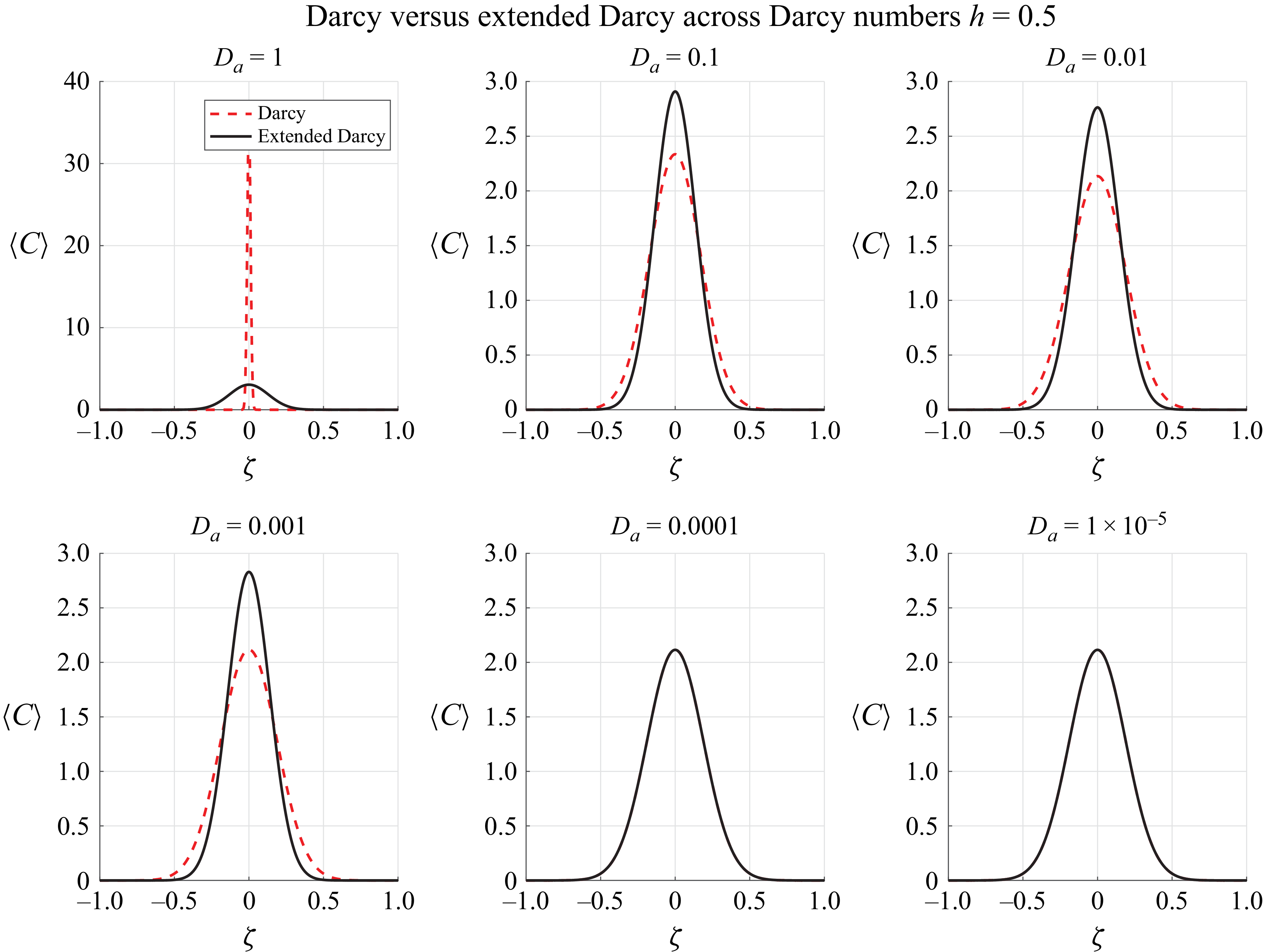
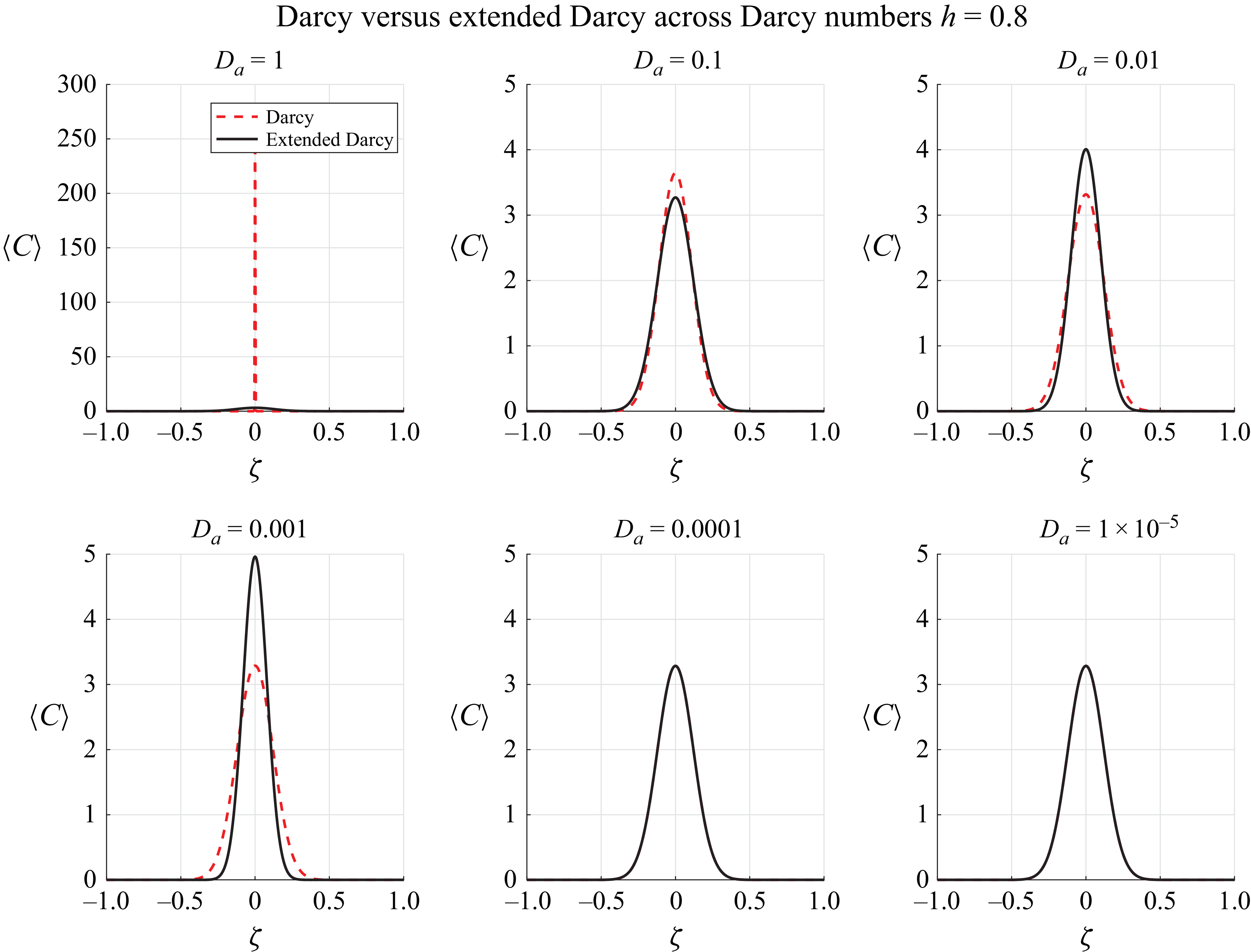
In figures 16 and 17, when
 $D_a = 1$
, the permeability
 $\kappa$
is such that the viscous penetration length
 $\ell _v \sim \sqrt {\kappa }$
is of order
 $H$
. This allows shear stresses from the free-fluid region to travel deep into the porous layer. The extended Darcy (Brinkman) model, which includes the
 $\mu _e{\nabla} ^2\boldsymbol{u}$
viscous diffusion term, transmits momentum into most of the porous thickness, sustaining a small but finite velocity there and enhancing cross-layer advection.The classical Darcy model neglects viscous shear inside the porous medium, producing a rapid velocity drop near the interface and confining solute transport largely to the free-fluid core. Because
 $h$
is larger than in figure 15, the effect of Brinkman shear penetration is more pronounced, yielding broader
 $\langle C \rangle (\zeta )$
profiles and a lower centreline peak.
Darcy versus extended Darcy, where
 $h=0.5$
,
 $M=1.05$
,
 $Q=1$
,
 $t^*=1$
.
Darcy versus extended Darcy, where
 $h=0.8$
,
 $M=1.05$
,
 $Q=1$
,
 $t^*=1$
.
For
 $D_a = 0.1$
and
 $0.01$
, the viscous penetration length
 $\ell _v$
decreases but remains greater than
 $h$
, allowing shear penetration to influence the entire porous layer. The Brinkman model still produces smoother gradients at the fluid–porous interface and broader concentration distributions than the Darcy model.
At low
 $D_a$
, permeability is small and the drag term dominates. In the Darcy model the porous layer becomes nearly stagnant, resulting in a steep drop in concentration near the wall. The extended Darcy model still predicts slightly higher near-wall concentrations due to limited shear penetration, but the differences are smaller than at high
 $D_a$
. For
 $h = 0.5$
, this weak advection effect remains more visible than in a thinner layer (figure 15).
Increasing
 $h$
amplifies the impact of the Brinkman term at all Darcy numbers (figures 15, 16 and 17). For thick layers (
 $h = 0.8$
), shear penetration influences a large volume of the porous medium, producing pronounced differences between the models across the entire
 $D_a$
range. For moderate thickness (
 $h = 0.5$
), the differences are still substantial at high
 $D_a$
and remain visible at low
 $D_a$
. Thin layers (
 $h = 0.3$
) show the smallest – but still non-negligible – differences, particularly at high
 $D_a$
where
 $\ell _v \gtrsim h$
.
The extended Darcy (Brinkman) formulation is the physically consistent choice whenever (i)
 $D_a \gtrsim h^2$
or (ii)
 $h$
is large enough for shear penetration to influence dispersion. The classical Darcy model is only adequate for thin layers with low permeability, where shear effects are negligible.
5. Conclusion
This comprehensive study investigates the intricate dynamics of a two-layered channel flow featuring dispersion in composite media within its layers. By formulating mass transport accurately, using fundamental momentum and solute transport equations adapted for two-layered channels, our research unveils critical implications for many applications. Mei’s perturbation analysis for fluid dispersion in a single-layer channel has been extend for our insights in a two-zone channel flow, deriving an expression for concentration variation. Introducing distinct time scales for convection and diffusion processes, we consider the characteristic length and height of the channel, constructing two-time coordinates. Concentration has also been subjected to a similar two-scale expansion. The velocity profile for fully developed flow through a two-layered channel is derived as a specific case, revealing that velocity decreases as the height of the porous layer increases; moreover, an increase in Darcy number and pressure gradient results in an escalation of velocity. Dispersion dynamics is scrutinised, with dispersivity found to be contingent on the height of the porous region. As the Péclet number of fluid regions and the pressure gradient rises, dispersivity increases, while higher Darcy numbers yield flatter dispersivity trends. The mean concentration distribution is shown to impact the height of the porous region and decreases the peak of the concentration graph with an increase in pressure gradient. A two-dimensional concentration plot is presented, highlighting the effects of various parameters. A comparative analysis with results from a single-layer channel flow and the velocity profile for a specific case, along with dispersivity in a two-layer channel flow, reinforces the robustness of our findings. We also compared the analytical results with numerical solutions obtained using the finite difference method up to the second-order approximation, and found a close agreement between the two. In conclusion, our study provides a nuanced understanding of the multi-layered channel flow dynamics, offering valuable insights for diverse applications such as, for example, groundwater pollution. The meticulous comparison of our results with computational methods and existing literature underscores the significance and novelty of our contributions. We also determine the velocity profile, dispersion coefficient and mean concentration using the classical Darcy model for the porous region. The findings indicate that the classical Darcy model provides better accuracy compared with the extended Darcy model, especially in cases when the porous region is thin and has low permeability; in other cases the extended Darcy model is better suited.
Supplementary material
Supplementary material is available at https://doi.org/10.1017/jfm.2025.10691.
Acknowledgements
The authors extend their heartfelt gratitude to the referees for offering valuable suggestions to enhance the paper.
Funding
This research received no specific grant from any funding agency, commercial or not-for-profit sectors.
Declaration of interests
The authors report no conflict of interest.
Appendix A.
The complete mathematical expressions of
 $I_{1}$
,
 $I_{2}$
,
 $I_{3}(y)$
,
 $I_{4}(y)$
,
 $I_{5}$
to
 $I_{8}$
, and,
 $d_{3}$
to
 $d_{16}$
, as introduced in subsection (3.2), are presented as follows:
 \begin{align} I_1 = &-\dfrac {1}{6} D_a Q (D_a Q - \langle u \rangle ) \left(-h^3 + 6 (D_a M)^{3/2} \sinh \left (\frac {h}{\sqrt {D_a M}}\right )\right) \nonumber \\ &+ \dfrac {1}{2} d_2 \sqrt {D_a M} (D_a Q - \langle u \rangle ) \left(-h^2 - 2 D_a M + 2 D_a M \cosh \left (\frac {h}{\sqrt {D_a M}}\right)\right) \nonumber \\ &+ d_3 D_a h Q - d_3 h \langle u \rangle - \dfrac {1}{6} D_a h^3 Q \langle u \rangle + \frac {h^3 \langle u \rangle ^2}{6} \nonumber \\ &+ \dfrac {1}{4} D_a^2 Q^2 \left ( 2 D_a h M + 4 D_a h M \cosh \left (\frac {h}{\sqrt {D_a M}}\right ) \right . \nonumber \\ & + 2 \sqrt {D_a M} \left(-h^2 - 2 D_a M + D_a M \cosh \left (\frac {h}{\sqrt {D_a M}}\right )\right) \sinh \left (\frac {h}{\sqrt {D_a M}}\right)\!\bigg) \nonumber \\ &- \dfrac {1}{2} D_a Q \left ( -2 d_2 (D_a M)^{3/2} + 2 D_a M (d_2 \sqrt {D_a M} + h \langle u \rangle ) \cosh \left (\frac {h}{\sqrt {D_a M}}\right ) \right . \nonumber \\ &\quad - (2 d_2 D_a h M + \sqrt {D_a M} (-2 d_3 + h^2 \langle u \rangle + 2 D_a M \langle u \rangle ) \sinh \left (\frac {h}{\sqrt {D_a M}}\right ) \nonumber \\ &\quad + d_2 (D_a M)^{3/2} \sinh \left (\frac {h}{\sqrt {D_a M}}\right )^2 \bigg ) \nonumber \\ &+ \dfrac {1}{2} d_2 D_a Q \left ( \sqrt {D_a M} (h^2 + 2 D_a M) \cosh \left (\frac {h}{\sqrt {D_a M}}\right ) \right . \nonumber \\ &\quad - (D_a M)^{3/2} \sinh \left (\frac {h}{\sqrt {D_a M}}\right )^2 \nonumber \\ &\quad - 2 D_a M \left(\sqrt {D_a M} + h \sinh \left (\frac {h}{\sqrt {D_a M}}\right )\right) \bigg ) \nonumber \\ &+ \dfrac {1}{4} d_2 \left ( -2 d_2 D_a h M - 4 d_3 \sqrt {D_a M} + 4 (D_a M)^{3/2} \langle u \rangle \right . \nonumber \\ &\quad - 2 (2 d_2 D_a h M + \sqrt {D_a M} (-2 d_3 + h^2 \langle u \rangle + 2 D_a M \langle u \rangle )) \cosh \left (\frac {h}{\sqrt {D_a M}}\right ) \nonumber \\ &\quad + 4 D_a M (d_2 \sqrt {D_a M} + h \langle u \rangle ) \sinh \left (\frac {h}{\sqrt {D_a M}}\right ) \nonumber \\ &\quad + d_2 (D_a M)^{3/2} \sinh \left (\frac {2h}{\sqrt {D_a M}}\right)\!\bigg), \end{align}
 \begin{align} I_2=\frac {1}{5040} \Bigg [ &-252 d_1^2 - 132 Q^2 - h \left ( h \left ( 84 d_1^2 (-15 + 20 h - 10 h^2 + 2 h^3) \right . \right . \nonumber \\ & + 3 (-140 + 70 h + 70 h^2 - 49 h^3 + 5 h^5) Q^2 \nonumber \\ & - 7 d_1 \left ( (-210 + 200 h - 15 h^2 - 42 h^3 + 15 h^4) Q \right . \nonumber \\ & + 60 (9 - 8 h + 2 h^2) (-1 + \langle u \rangle ) \Big ) \nonumber \\ & \left . + \, 42 (50 - 20 h - 15 h^2 + 7 h^3) Q (-1 + \langle u \rangle ) \right . \nonumber \\ & \left . + \, 840 (-3 + h) (-1 + \langle u \rangle )^2 \right ) \nonumber \\ & + 840 d_4 \left ( 6 + 3 d_1 (-2 + h) - (-3 + h^2) Q - 6 \langle u \rangle \right ) \Bigg ] \nonumber \\ & + 28 d_1 (45 + 13 Q - 45 \langle u \rangle ) \nonumber \\ & + 840 d_4 (6 - 3 d_1 + 2 Q - 6 \langle u \rangle ) \nonumber \\ & + 924 Q (-1 + \langle u \rangle ) - 1680 (-1 + \langle u \rangle )^2, \end{align}
 \begin{align} I_3(y) = &\dfrac {1}{2} {\textit{Pe}}_p \left ( \frac {1}{12} (D_a Q - \langle u \rangle )^2 y^4 - \frac {1}{3} d_2 \sqrt {D_a M} (D_a Q - \langle u \rangle ) y^3 \right . \nonumber \\ &- \dfrac {1}{2} \left (-M Q^2 D_a^3 + d_2^2 M D_a - 2 d_3 {\textit{QD}}_a + 2 d_3 \langle u \rangle \right ) y^2 \nonumber \\ &- 2 D_a M \left (M Q^2 D_a^3 - M Q \langle u \rangle D_a^2 - d_2^2 M D_a + d_2 \sqrt {D_a M} Q y D_a \right . \nonumber \\ &\left .- d_2 \sqrt {D_a M} \langle u \rangle y\right ) \cosh \left ( \frac {y}{\sqrt {D_a M}} \right ) \nonumber \\ &- D_a \sqrt {D_a M} \left (-2 M \sqrt {D_a M} d_2^2 - 2 M \langle u \rangle y d_2 + 6 D_a^2 M \sqrt {D_a M} Q^2 \right . \nonumber \\ &+ D_a \sqrt {D_a M} Q^2 y^2 - \sqrt {D_a M} Q \langle u \rangle y^2 + 2 d_3 \sqrt {D_a M} Q \nonumber \\ &\left .- 6 D_a M \sqrt {D_a M} Q \langle u \rangle \right ) \cosh \left ( \frac {y}{\sqrt {D_a M}} \right ) \nonumber \\ &+ \dfrac {1}{4} D_a^2 M^2 \left (d_2^2 + D_a^2 Q^2\right ) \cosh \left ( \frac {2y}{\sqrt {D_a M}} \right ) \nonumber \\ &- 2 D_a M \sqrt {D_a M} \left (-D_a^2 y Q^2 + D_a \langle u \rangle y Q + d_2 \sqrt {D_a M} \langle u \rangle \right ) \sinh \left ( \frac {y}{\sqrt {D_a M}} \right ) \nonumber \\ &+ D_a M \left (-2 \sqrt {D_a M} y d_2^2 + D_a Q y^2 d_2 - \langle u \rangle y^2 d_2 + 2 d_3 d_2 \right . \nonumber \\ &+ 4 D_a^2 M Q d_2 - 6 D_a M \langle u \rangle d_2 + 2 D_a^2 \sqrt {D_a M} Q^2 y \nonumber \\ &\left .- 2 D_a \sqrt {D_a M} Q \langle u \rangle y\right ) \sinh \left ( \frac {y}{\sqrt {D_a M}} \right ) \nonumber \\ &\left .- \dfrac {1}{2} d_2 D_a^3 M^2 Q \sinh \left ( \frac {2y}{\sqrt {D_a M}} \right ) \right )\!, \end{align}
 \begin{align} I_4(y) = &\frac {{\textit{Pe}}_{\!f}}{5040} \left ( \frac {15 Q^2 y^8}{8} - 15 d_1 Q y^7 \right . \nonumber \\ &+ \frac {7}{2} \left (8 d_1^2 + 14 Q d_1 - 7 Q (Q - 2 \langle u \rangle + 2)\right ) y^6 \nonumber \\ &+ 21 \left (-8 d_1^2 + (Q - 8 \langle u \rangle + 8) d_1 + 2 Q (Q - 3 \langle u \rangle + 3)\right ) y^5 \nonumber \\ &+ \frac {35}{2} \left (24 d_1^2 - 4 (5 Q - 12 \langle u \rangle + 12) d_1 \right . \nonumber \\ &\left .+ 3 \left (Q^2 - 4 (d_4 + \langle u \rangle - 1) Q + 4 (\langle u \rangle - 1)^2\right )\right ) y^4 \nonumber \\ &- 70 \left (6 d_1^2 - (12 d_4 + 7 Q - 18 \langle u \rangle + 18) d_1 \right . \nonumber \\ &\left .+ 2 \left (Q^2 - 5 (\langle u \rangle - 1) Q + 6 (\langle u \rangle - 1)^2\right )\right ) y^3 \nonumber \\ &+ 1260 d_4 (-2 d_1 + Q - 2 \langle u \rangle + 2) y^2 \left . \right )\!, \end{align}
 \begin{align} &I_5 = \frac {h}{{\textit{Pe}}_p} - \frac {1}{{\textit{Pe}}_p} - {\textit{Pe}}_p \left ( \frac {h^3 \langle u \rangle ^2}{6} - d_2 d_3 \sqrt {D_a M} + \frac {D_a^2 Q^2 h^3}{6} - d_3 h \langle u \rangle - \frac {D_a M d_2^2 h}{2} \right . \nonumber \\ & \left . - \frac {D_a Q h^3 \langle u \rangle }{3} + \frac {d_2 h^2 \langle u \rangle \sqrt {D_a M}}{2} + \frac {D_a^3 {\textit{MQ}}^2 h}{2} + D_a Q d_3 h + d_2 d_3 \cosh \!{\left (\!\frac {h}{\sqrt {D_a M}}\!\right )} \sqrt {D_a M} \right . \nonumber \\[5pt] & \left . + 2 D_a M d_2 \langle u \rangle \sqrt {D_a M} - D_a Q d_3 \sinh {\left (\frac {h}{\sqrt {D_a M}}\right )} \sqrt {D_a M} - \frac {D_a^2 M Q d_2 \sqrt {D_a M}}{2} \right . \nonumber \\ & \left . - \frac {D_a^2 Q^2 h^2 \sinh {\left (\!\dfrac {h}{\sqrt {D_a M}}\!\right )} \sqrt {D_a M}}{2} - \frac {D_a Q d_2 h^2 \sqrt {D_a M}}{2} + D_a M d_2^2 \sinh \!{\left (\!\frac {h}{\sqrt {D_a M}}\!\right )} \sqrt {D_a M} \right . \nonumber \\ & \left . + \frac {D_a M d_2^2 \sinh {\left (\dfrac {2h}{\sqrt {D_a M}}\right )} \sqrt {D_a M}}{4} - D_a M d_2^2 h \cosh {\left (\frac {h}{\sqrt {D_a M}}\right )} \right . \nonumber \\ & \left . - \frac {d_2 h^2 \langle u \rangle \cosh {\left (\dfrac {h}{\sqrt {D_a M}}\right )} \sqrt {D_a M}}{2} - 2 D_a^3 M Q^2 \sinh {\left (\frac {h}{\sqrt {D_a M}}\right )} \sqrt {D_a M} \right . \nonumber \\ & \left . + \frac {D_a^3 M Q^2 \sinh {\left (\dfrac {2h}{\sqrt {D_a M}}\right )} \sqrt {D_a M}}{4} + D_a^3 M Q^2 h \cosh {\left (\frac {h}{\sqrt {D_a M}}\right )} \right . \nonumber \\ & \left . + \frac {D_a Q h^2 \langle u \rangle \sinh {\left (\dfrac {h}{\sqrt {D_a M}}\right )} \sqrt {D_a M}}{2} - 2 D_a M d_2 \langle u \rangle \cosh {\left (\frac {h}{\sqrt {D_a M}}\right )} \sqrt {D_a M} \right . \nonumber \\ & \left . + D_a M d_2 h \langle u \rangle \sinh {\left (\frac {h}{\sqrt {D_a M}}\right )} + D_a^2 M Q d_2 \cosh {\left (\frac {h}{\sqrt {D_a M}}\right )} \sqrt {D_a M} \right . \nonumber \\ & \left . - \frac {D_a^2 M Q d_2 \cosh {\left (\dfrac {2h}{\sqrt {D_a M}}\right )} \sqrt {D_a M}}{2} + \frac {D_a Q d_2 h^2 \cosh {\left (\dfrac {h}{\sqrt {D_a M}}\right )} \sqrt {D_a M}}{2} \right . \nonumber \\ & \left . + 2 D_a^2 M Q \langle u \rangle \sinh {\left (\frac {h}{\sqrt {D_a M}}\right )} \sqrt {D_a M} - D_a^2 M Q h \langle u \rangle \cosh {\left (\frac {h}{\sqrt {D_a M}}\right )} \right ) \nonumber \\ & - \frac {h - 1}{{\textit{Pe}}_{\!f}} + {\textit{Pe}}_{\!f} \left ( \frac {11 Q}{60} - \frac {d_1}{4} - d_4 - \frac {2 \langle u \rangle }{3} - \frac {13 Q d_1}{180} - \frac {Q d_4}{3} \right . \nonumber \\ & \left . - \frac {11 Q \langle u \rangle }{60} + \frac {d_1 d_4}{2} + d_4 h + \frac {d_1 \langle u \rangle }{4} + d_4 \langle u \rangle - \frac {5 Q h^2}{12} \right . \nonumber \\ & \left . + \frac {Q h^3}{6} + \frac {Q h^4}{8} - \frac {7 Q h^5}{120} + \frac {3 d_1 h^2}{4} - \frac {2 d_1 h^3}{3} + \frac {d_1 h^4}{6} + h^2 \langle u \rangle \right . \nonumber \\ & \left . - \frac {h^3 \langle u \rangle }{3} + \frac {11 Q^2}{420} + \frac {d_1^2}{20} - \frac {h^2}{2} + \frac {h^3}{6} + \frac {\langle u \rangle ^2}{3} - \frac {Q^2 h^2}{12} \right . \nonumber \\ & \left . + \frac {Q^2 h^3}{24} + \frac {Q^2 h^4}{24} - \frac {7 Q^2 h^5}{240} + \frac {Q^2 h^7}{336} - \frac {d_1^2 h^2}{4} + \frac {d_1^2 h^3}{3} \right . \nonumber \\ & \left . - \frac {d_1^2 h^4}{6} + \frac {d_1^2 h^5}{30} - \frac {h^2 \langle u \rangle ^2}{2} + \frac {h^3 \langle u \rangle ^2}{6} - \frac {3 d_1 h^2 \langle u \rangle }{4} + \frac {2 d_1 h^3 \langle u \rangle }{3} \right . \nonumber \\ & \left . - \frac {d_1 h^4 \langle u \rangle }{6} + \frac {Q d_4 h}{2} - d_1 d_4 h - d_4 h \langle u \rangle + \frac {7 Q d_1 h^2}{24} - \frac {5 Q d_1 h^3}{18} \right . \nonumber \\ & \left . + \frac {Q d_1 h^4}{48} + \frac {7 Q d_1 h^5}{120} - \frac {Q d_1 h^6}{48} - \frac {Q d_4 h^3}{6} + \frac {5 Q h^2 \langle u \rangle }{12} - \frac {Q h^3 \langle u \rangle }{6} \right . \nonumber \\ & \left . - \frac {Q h^4 \langle u \rangle }{8} + \frac {7 Q h^5 \langle u \rangle }{120} + \frac {d_1 d_4 h^2}{2} + \frac {1}{3} \right )\!, \end{align}
 \begin{align} &I_6 = \frac {h}{{\textit{Pe}}_p} - \frac {1}{{\textit{Pe}}_{\!f}} - {\textit{Pe}}_p \left ( \frac {h^3 \langle u \rangle ^2}{6} - d_2 d_3 \sqrt {D_a M} + \frac {D_a^2 Q^2 h^3}{6} - d_3 h \langle u \rangle - \frac {D_a M d_2^2 h}{2} \right . \nonumber \\ & \left . - \frac {D_a Q h^3 \langle u \rangle }{3} + \frac {d_2 h^2 \langle u \rangle \sqrt {D_a M}}{2} + \frac {D_a^3 {\textit{MQ}}^2 h}{2} + D_a Q d_3 h + d_2 d_3 \cosh \!{\left (\!\frac {h}{\sqrt {D_a M}}\!\right )} \sqrt {D_a M} \right . \nonumber \\ & \left . + 2 D_a M d_2 \langle u \rangle \sqrt {D_a M} - D_a Q d_3 \sinh \!{\left (\!\frac {h}{\sqrt {D_a M}}\!\right )} \sqrt {D_a M} - \frac {D_a^2 M Q d_2 \sqrt {D_a M}}{2} \right . \nonumber \\ & \left . - \frac {D_a^2 Q^2 h^2 \sinh {\left (\!\dfrac {h}{\sqrt {D_a M}}\!\right )} \sqrt {D_a M}}{2} - \frac {D_a Q d_2 h^2 \sqrt {D_a M}}{2} + D_a M d_2^2 \sinh {\left (\!\frac {h}{\sqrt {D_a M}}\!\right )} \sqrt {D_a M} \right . \nonumber \\ & \left . + \frac {D_a M d_2^2 \sinh {\left (\dfrac {2h}{\sqrt {D_a M}}\right )} \sqrt {D_a M}}{4} - D_a M d_2^2 h \cosh {\left (\frac {h}{\sqrt {D_a M}}\right )} \right . \nonumber \\ & \left . - \frac {d_2 h^2 \langle u \rangle \cosh {\left (\dfrac {h}{\sqrt {D_a M}}\right )} \sqrt {D_a M}}{2} - 2 D_a^3 M Q^2 \sinh {\left (\frac {h}{\sqrt {D_a M}}\right )} \sqrt {D_a M} \right . \nonumber \\ & \left . + \frac {D_a^3 M Q^2 \sinh {\left (\dfrac {2h}{\sqrt {D_a M}}\right )} \sqrt {D_a M}}{4} + D_a^3 M Q^2 h \cosh {\left (\frac {h}{\sqrt {D_a M}}\right )} \right . \nonumber \\ & \left . + \frac {D_a Q h^2 \langle u \rangle \sinh {\left (\dfrac {h}{\sqrt {D_a M}}\right )} \sqrt {D_a M}}{2} - 2 D_a M d_2 \langle u \rangle \cosh {\left (\frac {h}{\sqrt {D_a M}}\right )} \sqrt {D_a M} \right . \nonumber \\ & \left . + D_a M d_2 h \langle u \rangle \sinh {\left (\dfrac {h}{\sqrt {D_a M}}\right )} + D_a^2 M Q d_2 \cosh {\left (\frac {h}{\sqrt {D_a M}}\right )} \sqrt {D_a M} \right . \nonumber \\ & \left . - \frac {D_a^2 M Q d_2 \cosh {\left (\dfrac {2h}{\sqrt {D_a M}}\right )} \sqrt {D_a M}}{2} + \frac {D_a Q d_2 h^2 \cosh {\left (\dfrac {h}{\sqrt {D_a M}}\right )} \sqrt {D_a M}}{2} \right . \nonumber \\ & \left . + 2 D_a^2 M Q \langle u \rangle \sinh {\left (\frac {h}{\sqrt {D_a M}}\right )} \sqrt {D_a M} - D_a^2 M Q h \langle u \rangle \cosh {\left (\frac {h}{\sqrt {D_a M}}\right )} \right ) \nonumber \\ & - \frac {h - 1}{{\textit{Pe}}_{\!f}} + {\textit{Pe}}_{\!f} \left ( \frac {11 Q}{60} - \frac {d_1}{4} - d_4 - \frac {2 \langle u \rangle }{3} - \frac {13 Q d_1}{180} - \frac {Q d_4}{3} \right . \nonumber \\ & \left . - \frac {11 Q \langle u \rangle }{60} + \frac {d_1 d_4}{2} + d_4 h + \frac {d_1 \langle u \rangle }{4} + d_4 \langle u \rangle - \frac {5 Q h^2}{12} \right . \nonumber \\ & \left . + \frac {Q h^3}{6} + \frac {Q h^4}{8} - \frac {7 Q h^5}{120} + \frac {3 d_1 h^2}{4} - \frac {2 d_1 h^3}{3} + \frac {d_1 h^4}{6} + h^2 \langle u \rangle \right . \nonumber \\ & \left . - \frac {h^3 \langle u \rangle }{3} + \frac {11 Q^2}{420} + \frac {d_1^2}{20} - \frac {h^2}{2} + \frac {h^3}{6} + \frac {\langle u \rangle ^2}{3} - \frac {Q^2 h^2}{12} \right . \nonumber \\ & \left . + \frac {Q^2 h^3}{24} + \frac {Q^2 h^4}{24} - \frac {7 Q^2 h^5}{240} + \frac {Q^2 h^7}{336} - \frac {d_1^2 h^2}{4} + \frac {d_1^2 h^3}{3} \right . \nonumber \\ & \left . - \frac {d_1^2 h^4}{6} + \frac {d_1^2 h^5}{30} - \frac {h^2 \langle u \rangle ^2}{2} + \frac {h^3 \langle u \rangle ^2}{6} - \frac {3 d_1 h^2 \langle u \rangle }{4} + \frac {2 d_1 h^3 \langle u \rangle }{3} \right . \nonumber \\ & \left . - \frac {d_1 h^4 \langle u \rangle }{6} + \frac {Q d_4 h}{2} - d_1 d_4 h - d_4 h \langle u \rangle + \frac {7 Q d_1 h^2}{24} - \frac {5 Q d_1 h^3}{18} \right . \nonumber \\ & \left . + \frac {Q d_1 h^4}{48} + \frac {7 Q d_1 h^5}{120} - \frac {Q d_1 h^6}{48} - \frac {Q d_4 h^3}{6} + \frac {5 Q h^2 \langle u \rangle }{12} - \frac {Q h^3 \langle u \rangle }{6} \right . \nonumber \\ & \left . - \frac {Q h^4 \langle u \rangle }{8} + \frac {7 Q h^5 \langle u \rangle }{120} + \frac {d_1 d_4 h^2}{2} + \frac {1}{3} \right )\!, \end{align}

 \begin{align} & \quad + \frac {d_1^2 h^2 \langle u \rangle ^2}{6} + d_4^2 h^3 \langle u \rangle + d_4 h^3 \langle u \rangle + d_1 h^4 \langle u \rangle - d_1 d_4 h^4 \langle u \rangle + d_1 d_4 h^4 \langle u \rangle \nonumber \\ & \quad + d_4^2 h^3 \langle u \rangle ^2 + \frac {d_1^2 h^4 \langle u \rangle ^2}{12} - \frac {d_1 d_4^2 h^4 \langle u \rangle ^2}{12} + d_1 d_4^2 h^3 \langle u \rangle + d_1^2 d_4^2 h^2 \langle u \rangle ^2 + d_4^2 h^4 \langle u \rangle ^2 \bigg ) \nonumber \\ & \quad - \frac {d_1 d_4 h^2}{2} + \frac {d_1^2 h^2}{4} + \frac {d_1 d_4 h^3}{12} - \frac {d_4^2 h^4}{12} + d_1^2 h^2 - d_1 h^3 + d_4 h^4 \nonumber \\ & \quad + \frac {h^2 d_1^2}{4} + d_1^2 d_4 h^2 + \frac {h^2 d_4^2}{12} + d_4^2 h^4 + d_4^2 h^3, \end{align}
 \begin{align} I_8 = &\, \frac {1}{336}\bigg (-{Q^2 h^6 + Q(Q - 7d_1)h^5 + \left (-\frac {44Q^2}{5} - \frac {98}{5} + \frac {63d_1}{5} + \frac {84 \langle u \rangle }{5}\right )h^4} \nonumber \\ &+ \left (\frac {26Q^2}{5} + \frac {98d_1}{5} - \frac {126 \langle u \langle }{5} + \frac {112}{5}\right )Qh^3 \nonumber \\ &+ \left (\frac {96Q^2}{5} + \frac {392}{5} - \frac {1106d_1}{15} - \frac {266 \langle u \rangle }{5} - 56d_4\right )Qh^2 \nonumber \\ &+ \left (-\frac {44Q^2}{5} - \frac {308}{5} - 56d_4 + \frac {154 \langle u \rangle }{5} + \frac {364d_1}{15}\right )Qh - \frac {84d_1^2}{5} + 84 + 168d_4 - 42 \langle u \rangle \nonumber \\ &- \frac {44Q^2}{5} + \frac {364d_1}{15} + 112d_4 + \frac {154 \langle u \rangle }{5} - \frac {308}{5} - \frac {84d_1^2}{5} + \bigg (-168d_4 - 42 \langle u \rangle + 84 \bigg )d_1 \nonumber \\ &- 112 + 336d_4 + 112 \langle u \rangle (h - 1)\bigg ), \end{align}
 \begin{equation} d_3 = \frac {1}{{\textit{Pe}}_p}\{(1-h)(d_5{\textit{Pe}}_p-d_6{\textit{Pe}}_{\!f})-(d_7 {\textit{Pe}}_p + d_8 {\textit{Pe}}_{\!f})\}, \end{equation}
 \begin{equation} d_4 = -\frac {1}{{\textit{Pe}}_{\!f}}\{h(d_5{\textit{Pe}}_p-d_6{\textit{Pe}}_{\!f})+(d_7 {\textit{Pe}}_p + d_8 {\textit{Pe}}_{\!f})\}, \end{equation}
 \begin{align} d_5 &= QDa\left \{-\frac {h^2}{2}+MDa\cosh \left (\frac {h}{\sqrt {{\textit{MD}}_a}}\right )\right \} \nonumber\\&\quad +d_2\sqrt {{\textit{MD}}_a}\left (h-\sqrt {{\textit{MD}}_a}\sinh \left (\frac {h}{\sqrt {{\textit{MD}}_a}}\right )\right ) +\frac {\langle u \rangle }{2}h^2, \end{align}
 \begin{equation} d_6 = \left (h-\frac {h^2}{2}\right )-d_1\left (\frac {h}{2}-\frac {h^2}{2}+\frac {h^3}{6}\right )+\frac {Q}{2}\left (\frac {2h}{3}-\frac {h^2}{2}+\frac {h^4}{12}\right )-\langle u \rangle \left (h-\frac {h^2}{2}\right )\!, \end{equation}
 \begin{align} d_7 &= QDa\left (\frac {h^3}{6}-(\textit{MD}_a)^{3/2}\sinh \left (\frac {h}{\sqrt {{\textit{MD}}_a}}\right )\right )\nonumber\\&\quad +d_2\sqrt {MDa}\bigg (MDa\cosh \left (\frac {h}{\sqrt {{\textit{MD}}_a}}\right )-\frac {h^2}{2}-MDa\bigg )-\frac {\langle u\rangle }{6}h^3, \end{align}
 \begin{align} d_8 &= \left (-1+\frac {d_1}{2}-\frac {Q}{3}+\langle u \rangle \right )\frac {1-h^2}{2}+\left (\dfrac {1}{2}-\frac {d_1}{2}+\frac {Q}{4}-\frac {\langle u\rangle }{2}\right )\frac {1-h^3}{3}\nonumber\\&\quad +\frac {d_1}{24}\left (1-h^4\right )-\frac {Q}{120}\left (1-h^5\right )\!, \end{align}
 \begin{equation} d_9 = -{\textit{Pe}}_p \left ( d_2 \sqrt {D_a M} \left ( M {\textit{QD}}_a^2 - 2 M \langle u \rangle D_a + d_3 \right ) - D_a^2 M Q d_2 \sqrt {D_a M} \right )\!, \end{equation}
 \begin{equation} d_{10}=\frac {1}{{\textit{Pe}}_p}\{ d_{12}{\textit{Pe}}_{\!f} + (d_{14}-d_{13})\}, \end{equation}
 \begin{align} d_{11}&=-Pe\_{f} \left (\frac {Q^2}{336} - \frac {d_1Q}{48} - \frac {\left (1 - d_1 + \dfrac{Q}{2}\right )Q}{120} + \frac {d_1^2}{30} - \frac {Q\left (\dfrac {1}{2} - \dfrac{d_1}{2} + \dfrac{Q}{4} - \dfrac{\langle u \rangle }{2}\right)}{10} \right . \nonumber \\ &+ \left . \frac {\left (1 - d_1 + \dfrac{Q}{2}\right )d_1}{24} + \frac {d_1\left (\dfrac {1}{2} - \dfrac {d_1}{2} + \dfrac {Q}{4} - \dfrac { \langle u \rangle }{2}\right )}{4} - \frac {Q\left (u - \dfrac {Q}{3} + \dfrac {d_1}{2} - 1\right )}{8} \right . \nonumber \\ &+ \left . \frac {\left (1 - d_1 + \dfrac {Q}{2}\right )\left (\dfrac {1}{2} - \dfrac {d_1}{2} + \dfrac {Q}{4} - \dfrac {\langle u \rangle }{2}\right )}{3} + \frac {d_1\left (\langle u \rangle - \dfrac {Q}{3} + \dfrac {d_1}{2} - 1\right )}{3} - \frac {Qd_4}{6} \right . \nonumber \\ &+ \left . \frac {\left (1 - d_1 + \frac {Q}{2}\right )\left (u - \dfrac {Q}{3} + \dfrac {d_1}{2} - 1\right )}{2} + \dfrac {d_1d_4}{2} + \left (1 - d_1 + \frac {Q}{2}\right )d_4 \right )-I_6, \end{align}
 \begin{equation} d_{12}=\frac {1}{{\textit{Pe}}_{\!f}}\bigg [h\big(d_{13}-d_{14} \big)-\big(d_{15} + d_{16}\big)\bigg], \end{equation}
 \begin{equation} d_{13}={\textit{Pe}}_P\big(I_5h^2/2+I_3|_{y=h}+d_{9}h\big), \end{equation}
 \begin{equation} d_{14}={\textit{Pe}}_{\!f}\big(I_6h^2/2+I_4|_{y=h}+d_{11}h\big), \end{equation}
 \begin{equation} d_{15}={\textit{Pe}}_p \bigg ( I_5 \frac {h^3}{6}+I_7+d_9\frac {h^2}{2}\bigg ), \end{equation}
 \begin{equation} d_{16}={\textit{Pe}}_{\!f} \bigg ( I_6\frac {(1-h^3)}{6} +I_8+\frac {d_{11}}{2}(1-h^2)\bigg ). \end{equation}
Appendix B. Relationship between effective viscosity and slip model
Darcy’s law provides a fundamental description of flow through the porous region under slow, steady and creeping flow conditions. It is written as
 \begin{equation} U = -\frac {\kappa }{\mu } \frac {{\rm d}p}{{\rm d}x}, \end{equation}
where
 $U$
is the Darcy velocity defined as the volumetric flow rate per unit total cross-sectional area (including both solid and fluid phases). Here,
 $\kappa$
denotes the permeability of the medium,
 $\mu$
is the viscosity and
 ${\rm d}p/{\rm d}x$
is the pressure gradient.
However, within the pore space, the actual average velocity of the fluid, known as the interstitial velocity (
 $u_{\textit{int}}$
), is higher than the Darcy velocity and is defined as
 \begin{equation} u_{\textit{int}} = \frac {U}{\phi }, \end{equation}
where
 $\phi$
is the porosity, i.e. the fraction of the total volume occupied by voids. The distinction between
 $U$
and
 $u_{\textit{int}}$
becomes critical in modelling near-interface behaviour because the free-fluid region interacts directly with the pore-level velocity field, not with the averaged Darcy velocity.
To model the fluid–porous interface, Beavers & Joseph (Reference Beavers and Joseph1967) introduced an empirical slip boundary condition, which relates the tangential shear rate in the fluid to the difference between the slip velocity in the fluid (
 $u_s$
) and the interstitial velocity in the porous region (
 $u_{\textit{int}}$
), i.e.
 \begin{equation} \left . \frac {{\rm d}u}{{\rm d}y} \right |_{\textit{interface}} = \frac {\alpha }{\sqrt {\kappa }} (u_s - u_{\textit{int}}), \end{equation}
where
 $\alpha$
is the slip coefficient.
To model this interface behaviour using a more mechanistic framework, the extended Darcy model is used. This model adds a viscous shear term to Darcy’s law, resulting in
 \begin{equation} - \frac {{\rm d}p}{{\rm d}x} = \frac {\mu }{\kappa } u - \mu _{e} \frac {{\rm d}^2 u}{{\rm d}y^2}, \end{equation}
where
 $\mu _{e}$
is the effective viscosity in the porous region. It represents the resistance to tangential shear induced by the solid matrix of the porous medium. This term allows for a continuous velocity profile across the fluid–porous interface and models the smooth decay of velocity within the porous structure.
Solving (B4) in the porous region gives
 \begin{equation} u(y) = u_{\textit{int}} + (u_s - u_{\textit{int}}) \exp \left ( \frac {y}{\sqrt {\kappa } (\mu _{e} / \mu )} \right )\!, \end{equation}
subject to the following boundary conditions:
-
(i)
 $u(y \to -\infty ) \to u_{\textit{int}}$
,
-
(ii)
$u(y = 0) = u_s$
.


From (B5), the shear rate at the interface is
 \begin{equation} \left . \frac {{\rm d}u}{{\rm d}y} \right |_{y=0} = \frac {\mu }{\sqrt {\kappa } \mu _{\textit{e}}} (u_s - u_{\textit{int}}). \end{equation}
Comparing (B6) with the Beavers–Joseph condition (B3), we obtain
 \begin{equation} \alpha = \sqrt {\frac {\mu }{\mu _{\textit{e}}}}. \end{equation}
This identity shows that the effective viscosity model and the slip model are physically and mathematically consistent. While the slip coefficient
 $\alpha$
is obtained from experiments, the extended Darcy model embeds this behaviour into the governing equations through
 $\mu _{\textit{e}}$
, allowing a more systematic treatment in analytical and numerical modelling.
This equivalence also justifies the use of
 $\mu _{\textit{e}}$
in the porous region as a mathematically robust and physically interpretable parameter to model near-interface velocity behaviour in layered systems.
Appendix C. Physical significance of effective viscosity in the Darcy–Brinkman equation
To accurately capture the momentum transport near porous–fluid interfaces, particularly in highly porous systems, the Darcy–Brinkman model introduces an effective viscosity, which extends the classical Darcy law by incorporating a viscous shear term. The effective viscosity arises in the modelling parameter of fluid flow through porous or composite media, especially in regions adjacent to interfaces between free fluid and porous layers. The effective viscosity value is not universal, it depends on the geometry, type of fluid, porosity, permeability of the medium and structure of the porous medium and often requires experimental and numerical (Hazra et al. Reference Hazra, Class, Helmig and Schulz2004) fitting . In practical applications,
 $\mu _{e}$
is often treated as an adjustable fitting parameter to match experimental data or to ensure continuity of velocity and stress across interfaces. Although not physically measurable like true viscosity, it is widely accepted in engineering and computational modelling due to its ability to approximate realistic interfacial behaviour in complex porous systems. The term
 $\mu _e {\nabla} ^2 u$
represents the viscous shear contribution in the Darcy–Brinkman equation and facilitates the imposition of a no-slip velocity condition on solid boundaries. Clearly when
 $ u=0$
, the Darcy–Brinkman equation reduces to the Darcy equation.
C.1. Effective viscosity
$\mu _e$
versus viscosity
$\mu$


Brinkman’s original work suggested that
 $\mu _e$
could be approximated using Einstein’s formula, i.e.
 \begin{equation} \frac {\mu _e}{\mu } \approx 1 + \frac {5}{2}(1 - \phi ), \end{equation}
where
 $\phi$
is the porosity. However, later theoretical and experimental studies demonstrated that
 $\mu _e$
may be higher or lower than
 $\mu$
depending on the pore structure. Koplik, Levine & Zee (Reference Koplik, Levine and Zee1983) found that
 $\mu _e \lt \mu$
for low porosities, while Durlofsky & Brady (Reference Durlofsky and Brady1987) and Martys et al. (Reference Martys, Bentz and Garboczi1994) reported
 $\mu _e \gt \mu$
in more permeable media. Ochoa-Tapia & Whitaker (Reference Ochoa-Tapia and Whitaker1995) suggested
 $\mu _e = \mu /\phi$
, a simple empirical relation validated in several studies.
At interfaces between porous and clear fluid regions,
 $\mu _e$
is crucial for ensuring continuity of velocity and shear stress. If
 $\mu _e \neq \mu$
, a stress jump condition may be required, which is proposed by Ochoa-Tapia & Whitaker (Reference Ochoa-Tapia and Whitaker1995). Givler & Altobelli (Reference Givler and Altobelli1994) used Nuclear Magnetic Resonance to measure velocity profiles in open-cell foams with
 $\phi = 0.972$
and found
 $\mu _e \approx 7.5 \mu$
. Other studies have reported values from
 $0.5 \mu$
to
 $3 \mu$
, depending on the pore structure.
Alazmi & Vafai (Reference Alazmi and Vafai2001) found that variations in
 $\mu _e$
had minor effects on velocity and heat transfer in certain regimes, though they may be significant near interfaces.
We can conclude that the effective viscosity
 $\mu _e$
in the Darcy–Brinkman equation is essential for modelling shear effects in porous media and ensuring realistic interface behaviour. While often approximated as
 $\mu$
, its actual value depends on porosity and structure of the geometry and should be determined from theory or experiments when precision is required.
Appendix D. Two-dimensional transport model, including influence of two-dimensional advection
The general solutions of velocities of porous and fluid media are (which we previously obtained in (3.3)–(3.6))
 \begin{equation} u_p(y) = \textit{QD}_a \left (1-\cosh \left \{\frac {y}{\sqrt {{\textit{MD}}_a}}\right \}\right ) +d_2\sinh \left \{\frac {y}{\sqrt {{\textit{MD}}_a}}\right \} \end{equation}
and
 \begin{equation} u_{\!f}(y) = 1- d_1(1-y) +\frac {Q}{2}(1-y^2), \end{equation}
where
 $d_1$
and
 $d_2$
are given as
 \begin{equation} d_1 = d_2\sqrt {\frac {M}{D_a}}\cosh \left \{\frac {1}{\sqrt {{\textit{MD}}_a}}h\right \}-Q\sqrt {{\textit{MD}}_a}\sinh \left \{\frac {1}{\sqrt {{\textit{MD}}_a}}h\right \}+ hQ, \end{equation}
 \begin{equation} d_2 = \frac {1+\frac {1}{2}Q(1-h)^2 -{\textit{QD}}_a\left (1-\cosh \left \{\dfrac {1}{\sqrt {{\textit{MD}}_a}}h\right \}\right ) +(1-h)Q\sqrt {{\textit{MD}}_a}\sinh \left\{\dfrac {1}{\sqrt {{\textit{MD}}_a}}h\right\}}{\sinh \left \{\dfrac {1}{\sqrt {{\textit{MD}}_a}}h\right \} + \sqrt {\dfrac {M}{D_a}}(1-h)\cosh \left \{\dfrac {1}{\sqrt {{\textit{MD}}_a}}h\right \}}. \end{equation}
To find transverse velocity, we use equation of continuity,
 \begin{equation} \frac {\partial u}{\partial x} + \frac {\partial v}{\partial y}=0. \end{equation}
But in our case this is not possible, as using the equation of continuity, we get
 $v=0$
, which is obvious, as we assume fully developed flow, so for finding transverse velocity, let us assume very slight axial variation in
 $u$
,
 \begin{equation} u(x,y)=u(y)(1+ \epsilon _{1} x), \end{equation}
where
 $\epsilon _{1}$
is a parameter. Then we use the equation of continuity and we get the transverse velocity profiles for porous and fluid media:
 \begin{align}&\qquad\qquad\qquad v_p(y)=-\epsilon _{1}[y-d_1\left(y-\frac {y^2}{2}+\frac {Q}{2}\left(y-\frac {y^3}{3}\right)\right)\!, \end{align}
 \begin{align}& v_{\!f}(y)=-\epsilon _{1}[\textit{QD}_a(y-\sqrt {{\textit{MD}}_a} \sinh \left(\frac {y}{\sqrt (\textit{MD}_a)}\right)+d_2 \sinh \left(\frac {y}{\sqrt (\textit{MD}_a)}\right)+C_2. \end{align}
Here
 \begin{equation} C_2= 1+\epsilon _{1}(\textit{QD}_a(1-\sqrt {{\textit{MD}}_a}\sinh \left(\frac {1}{\sqrt {{\textit{MD}}_a}}+d2\sqrt {{\textit{MD}}_a}\cosh \left(\frac {1}{\sqrt {{\textit{MD}}_a}}\right)\right)\!. \end{equation}
After non-dimensionalisation in terms of space and time, the advection–diffusion equations and the associated initial and boundary conditions can be reformulated in terms of dimensionless space and time variables
 $\{\zeta ,t^*\}$
as
 \begin{align}& {\textit{Pe}}_p\langle \frac {1}{\textit{Pe}}\rangle \frac {\partial C_{\!p}}{\partial t^*}+{\textit{Pe}}_p(u_p-\langle u \rangle )\frac {\partial C_{\!p}}{\partial \zeta }+{\textit{Pe}}_pv_p\frac {\partial C_{\!p}}{\partial y}=\frac {\partial ^2 C_{\!p}}{\partial \zeta ^2} + \frac {\partial ^2 C_{\!p}}{\partial y^2}, \quad 0\lt y\leqslant h, \end{align}
 \begin{align}& {\textit{Pe}}_{\!f}\langle \frac {1}{\textit{Pe}}\rangle \frac {\partial C_{\!f}}{\partial t^*}+{\textit{Pe}}_{\!f}(u_{\!f}-\langle u \rangle )\frac {\partial C_{\!f}}{\partial \zeta }+{\textit{Pe}}_{\!f}v_{\!f}\frac {\partial C_{\!p}}{\partial y}=\frac {\partial ^2 C_{\!f}}{\partial \zeta ^2} + \frac {\partial ^2 C_{\!f}}{\partial y^2},\quad h \leqslant y\lt 1, \end{align}
 \begin{align}&\qquad\qquad\qquad\qquad\qquad C_{\!p}(\zeta ,y,t^*)\mid _{t^*=0} = \delta (\zeta ),\quad 0\lt y \leqslant h, \end{align}
 \begin{align}&\qquad\qquad\qquad\qquad\qquad C_{\!f}(\zeta ,y,t^*)\mid _{t^*=0} = \delta (\zeta ),\quad h\leqslant y\lt 1, \end{align}
 \begin{align}&\qquad\qquad\qquad\qquad\qquad\qquad \frac {\partial C_{\!p}}{\partial y}\bigg {|}_{y=0} = \frac {\partial C_{\!f}}{\partial y}\bigg {|}_{y=1} = 0, \end{align}
 \begin{align}&\qquad\qquad\qquad\qquad\qquad\qquad\quad C_{\!p} \mid _{y=h} = C_{\!f} \mid _{y=h}, \end{align}
and
 \begin{align}&\quad\,\, \frac {1}{{\textit{Pe}}_{p}}\frac {\partial C_{\!p}}{\partial y}\bigg {|}_{y=h} = \frac {1}{{\textit{Pe}}_{\!f}}\frac {\partial C_{\!f}}{\partial y}\bigg {|}_{y=h}, \end{align}
 \begin{align}& C_{\!p}(\zeta ,y,t^*)\mid _{\zeta \rightarrow \pm \infty } = 0,\quad 0\lt y \leqslant h, \end{align}
 \begin{align}& C_{\!f}(\zeta ,y,t^*)\mid _{\zeta \rightarrow \pm \infty } = 0,\quad h\leqslant y \lt 1. \end{align}
To validate the accuracy of the analytical solution, we performed a numerical simulation for the system of (D10)–(D18). The rectangular domain used for discretisation has dimensions of 40 units in length and 1 unit in width, with the length spanning from –20 to 20 and the width ranging from 0 to 1. The unsteady terms in (D10) and (D11) are discretised using a first-order forward difference scheme, while the advection term is approximated with a first-order upwind scheme. For the axial and transverse diffusion terms, we applied a second-order central difference scheme to discretise the second derivatives. Since
 $v_p$
is not too large and accuracy is important, we use central difference. The resulting discretised governing equations, excluding the truncation error term, are given as
 \begin{align} & {\textit{Pe}}_p \left \langle \frac {1}{\textit{Pe}} \right \rangle \frac {C_{p_{i,j}}^{n+1} - C_{p_{i,j}}^{n}}{\Delta t^*} \nonumber \\ &\quad + {\textit{Pe}}_p \left \{ {\text{max}} (u_p - \langle u \rangle , 0) \frac {C_{p_{i,j}}^{n} - C_{p_{i-1,j}}^{n}}{\Delta \zeta } - {\text{max}} (\langle u \rangle - u_p, 0) \frac {C_{p_{i+1,j}}^{n} - C_{p_{i,j}}^{n}}{\Delta \zeta } \right \} \nonumber \\ &\quad+ v_p(i,j)\frac {C_{p_{i,j+1}}^{n} -C_{p_{i-1,j}}^{n}}{2 \Delta y} \nonumber \\ &\quad = \frac {C_{p_{i+1,j}}^{n} - C_{p_{i-1,j}}^{n}}{\Delta \zeta ^2}+\frac {C_{p_{i,j+1}}^{n} - 2C_{p_{i,j}}^{n} + C_{p_{i,j-1}}^{n}}{\Delta y^2}, \quad j=0,1,2,\ldots j_h, \end{align}
 \begin{align} & {\textit{Pe}}_{\!f} \left \langle \frac {1}{\textit{Pe}} \right \rangle \frac {C_{f_{i,j}}^{n+1} - C_{f_{i,j}}^{n}}{\Delta t^*} \nonumber \\ &\quad + {\textit{Pe}}_{\!f} \left \{ {\text{max}} (u_p - \langle u \rangle , 0) \frac {C_{f_{i,j}}^{n} - C_{f_{i-1,j}}^{n}}{\Delta \zeta } - {\text{max}} (\langle u \rangle - u_{\!f}, 0) \frac {C_{f_{i+1,j}}^{n} - C_{f_{i,j}}^{n}}{\Delta \zeta } \right \} \nonumber \\ &\quad+ v_{\!f}(i,j)\frac {C_{f_{i,j+1}}^{n} - C_{f_{i-1,j}}^{n}}{2 \Delta y} \nonumber \\ &\quad = \frac {C_{f_{i+1,j}}^{n} - 2C_{f_{i,j}}^{n} + C_{f_{i-1,j}}^{n}}{\Delta \zeta ^2}+\frac {C_{f_{i,j+1}}^{n} - 2C_{f_{i,j}}^{n} + C_{f_{i,j-1}}^{n}}{\Delta y^2}, \quad j=j_h,\ldots N_y. \end{align}
The boundary conditions in (D14) are discretised using three-point backward difference and forward difference schemes as
 \begin{equation} -3C_{p_{i,0}}+4C_{p_{i,1}}-C_{p_{i,2}}=0,\quad i=0,1,\ldots ,M_x, \end{equation}
and
 \begin{equation} 3C_{f_{i,N_y}}-4C_{f_{i,N_y-1}}+C_{p_{i,N_y-2}}=0,\quad i=0,1,\ldots ,M_x. \end{equation}
The discretised expression for the boundary conditions (D17) and (D18) are as follows:
 \begin{align} & C_{p_{0,j}}=0,\quad \textit{and} \quad C_{p_{M_x,j}}=0, \quad j=0,1,\ldots ,N_y, \end{align}
 \begin{align} & C_{f_{0,j}}=0, \quad \textit{and} \quad C_{f_{M_x,j}}=0, \quad j=0,1,\ldots ,N_y. \end{align}
The discretised expression of the initial conditions (D12) and (D13) are given as
 \begin{equation} C_{\!f}= C_{\!p}=\begin{cases} 0 \quad 0\leqslant i \leqslant M_x, 0\leqslant j \leqslant N_y, \quad i\neq M_x/2,& \nonumber \\ 50 \quad i=M_x/2, 0\leqslant j \leqslant N_y. \end{cases} \end{equation}
Comparison between the concentration profiles with and without transverse velocity at initial time (a)
 $t^*=0.1$
and (b)
 $t^*=0.5$
.
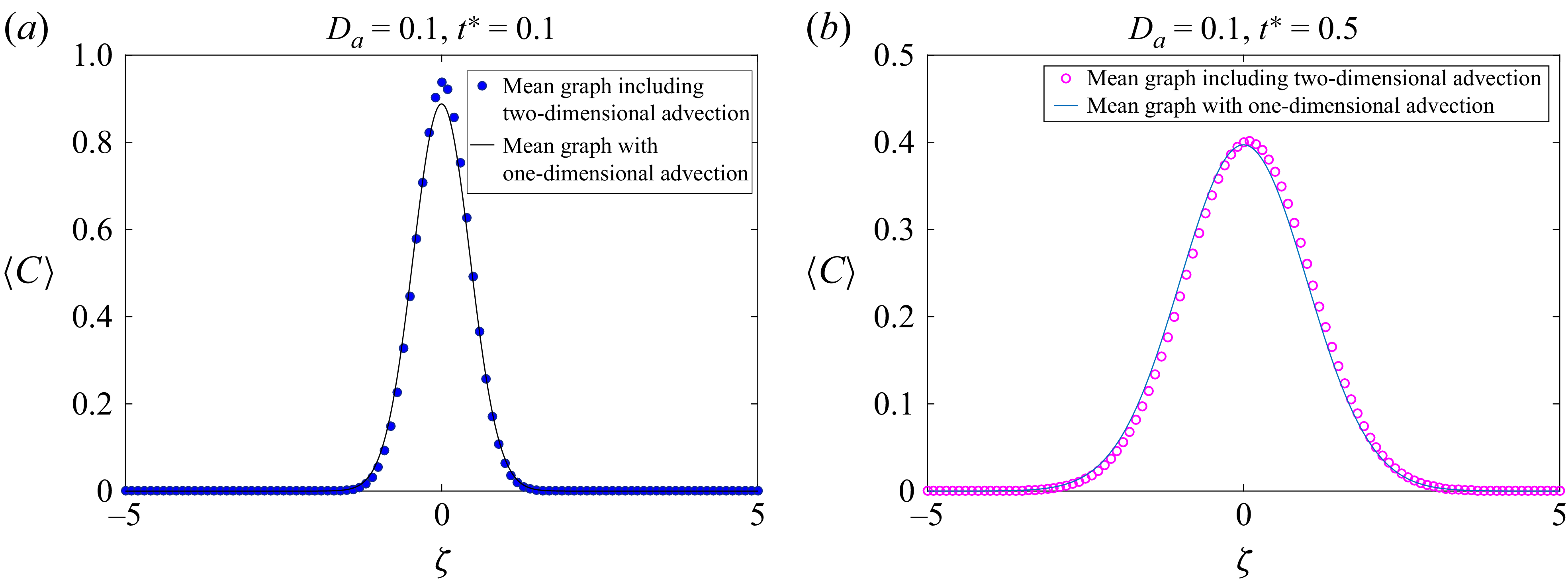
The figures present a comparison between the numerically computed two-dimensional concentration profile with transverse velocity and without transverse velocity for solute transport in a two-layered system. Both plots correspond to a fixed Darcy number of 0.1. Figures 18(a
) and 18(b) correspond to early time, the solute concentration exhibits a sharp and narrow peak near the centre of the domain. Figure 19 represents a later time, where the concentration profile becomes broader and the peak height decreases due to diffusion over time. For small
 $D_a$
, there is a negligible difference that diminishes as time as well as Darcy number increases. The solution without transverse velocity closely matches the transverse velocity result, suggesting that the simplified model remains accurate even at later stages of the transport process.
Comparison between the concentration profiles with and without transverse velocity at
 $t^*=1$
.