Nomenclature
- a i (t)
-
instantaneous amplitude
- c
-
acceleration factor
- E
-
total energy of the original signal
- E m
-
energy sum of each IMF component
- H(F, t)
-
Hilbert spectrum of the original signal
- i
-
number of the i-th particle
- I ef
-
excitation current on the AC exciter
- I F
-
current after rectification of the rotating rectifier
- j
-
j-th dimension
- K
-
modal decomposition number
- m i (t)
-
i-th modal component after decomposition
- n
-
number of intrinsic mode functions
- r
-
random numbers in the interval [0,1]
- r n (t)
-
residual component
- t
-
the number of iterations
- v ij
-
particle update rate
- w
-
inertia factor
- x ij
-
individual of particle swarm
- x(t)
-
original signal
- α
-
penalty factor
-
 ${\omega _i}(t)$
-
instantaneous frequency
- AGRR
-
aerospace generator rotating rectifier
- BLS
-
broad learning system
- ED
-
Euclidean distance
- EMD
-
empirical mode decomposition
- FFT
-
Fast Fourier transform
- HHT
-
Hilbert-Huang transform
- HAS
-
Hilbert spectrum analysis
- IMF
-
intrinsic mode function
- PHM
-
prognostic and health management
- PMG
-
permanent magnet generator
- PSO
-
particle swarm optimisation
- SAE
-
stacked auto-encoder
- TSBG
-
three-stage brushless AC generator
- VMD
-
variational mode decomposition

1.0 Introduction
With the development of aerospace science and multi-electric/all-electric technology, the traditional airborne pneumatic, hydraulic and mechanical power systems of aircraft are gradually being replaced by electrical energy (Reference Madonna, Giangrande and Galea1). In the aircraft power supply system, the main power supply is completed by the aerospace engine to drive the aerospace generator to generate electricity, which is used to supply power to electrical equipment on the aircraft. Therefore, the aircraft has high requirements for the stability and reliability of the power supply system. The generator, which is the main aerospace power, is an important guarantee for the energy supply and safety of airborne electrical equipment. Once the generator fails, it will have a serious impact on the safety of the entire aircraft system (Reference Wang, Nuzzo, Zhang, Zhao, Gerada and Galea2). Therefore, fault diagnosis is the key technology to ensure the reliability of aero-generators (Reference Kilic and Unal3).
At present, most of the aerospace generators use brushless AC synchronous generators. Such generators use rotating rectifiers to replace the traditional brushes and slip rings, which are an important part of the generator structure (Reference McArdle and Morrow4). Because the AGRR is located on the rotor, it rotates at a high speed with the rotor during operation and is frequently subjected to stress loads such as centrifugal force, voltage and current. Hence, this component fails easily (Reference Jiao, Han, Wei, Sun, Liang and Liu5). Experts have conducted much research on the Prognostic and Health Management (PHM) technology of the main power system (Reference Yin, Hu, Chen, Yang and Shen6–Reference Calabrese, Regattieri, Botti, Mora and Galizia8), and pointed out that the rotating rectifier fault is a key fault mode of the aerospace generator. To ensure the reliability of the generator’s operating state, the rotating diode needs to be monitored in a timely and effective manner in case of failure (Reference Salah, Bacha, Chaari and Benbouzid9).
The fault diagnosis technology of AGRR mainly consists of data acquisition, feature extraction and fault classification. Among them, fault feature extraction is the key technology of fault diagnosis, and can be summarised into several following categories:
-
(1) Methods based on modeling
This technology requires an in-depth analysis of the generator’s operating mechanism and knowledge of its parameter information to establish an accurate system model. For example, Reference (Reference Tantawy, Koutsoukos and Biswas10) develops a hybrid dynamic modeling method for generators based on phase domain representation for open-circuit faults of generator rotating rectifiers; Ref. (Reference TR, Kiran, Balasubramanian and Upendranath11) models the aircraft generator and its control system, and analyses the rotating rectifier and winding faults in the excitation circuit through this model. The study shows that the excitation current will change significantly when a single diode is open or short-circuited.
-
(2) Methods based on signal processing
For this method, it is necessary to process the collected generator fault signals by means of fast Fourier transform (FFT), wavelet transform or empirical mode decomposition (EMD) to obtain frequency domain or time-frequency domain information. For example, Ref. (Reference Jordan and Apsley12) studies the open-circuit fault of rectifier diode by spectrum analysis method. Reference (Reference Rahnama and Vahedi13) considers the excitation current, excitation voltage, generator output current and output voltage as the fault monitoring signal, and concludes that the excitation current is more suitable for the fault diagnosis of the AGRR through spectrum analysis. Reference (Reference Tang, Fan, Liu, Liu, Zhang and Bu14) adopts the HHT to process the output voltage of the rectifier for the open-circuit fault of the rotating diode, and then the Hilbert spectrum can distinguish the normal situation and the fault mode. In Ref. (Reference Yang, Peng, Wei, Shi and Tian15), VMD and EMD methods are used to extract instantaneous time-frequency features of signals, respectively, and experiments prove that VMD is better than EMD in terms of noise robustness and multicomponent signal decomposition. Reference (Reference Wang, Sun, Xiao and Lu16) proposes a denoising approach combining VMD with energy value (EV), simulation experiments demonstrate that the method of VMD-EV-VMD achieves a greater SNR than the methods of VMD, and it achieves a better denoising effect. Reference (Reference Zhang, Gao, Lu, Kong and Ma17) proposes a novel method based on fast iterative variational mode decomposition, and the simulation process shows FI-VMD is almost equivalent to the extraction accuracy of VMD, but when the energy of chatter signal is very small, FI-VMD is much better than VMD. In Ref. (Reference Pang, Liu, Wei, Sun, Jiao and Han18), the authors reconstruct the three-phase current on the rotor, and then use the amplitude ratio of the second harmonic of the current to the fundamental wave for fault detection, which can locate the fault of a single rotating diode. Reference (Reference Wei, Liu, Zhang, Jiao, Peng and Meng19) also analyses the harmonic components of the rotor current of the exciter and uses the ratios of the second to fourth harmonics to the fundamental wave as the fault features of the diagnostic diode.
-
(3) Data-driven methods
For an actual generator in operation, the fault signal collected through the measurable nodes may be inaccurate, and these signals may be subject to great interference and the fault characteristic information cannot be obtained by conventional methods. With the help of data-driven methods, such as neural networks, this problem can be solved. For example, Reference (Reference Cui, Tang, Gong and Zhang20) uses the stacked auto-encoder (SAE) method to adaptively extract fault features from the excitation current, and uses the classifier to classify the extracted features. Reference (Reference Cui, Feng, Zhang, Wang and Meng21) introduces the broad learning system (BLS) into the fault diagnosis of the rotating rectifier of aerospace generators, and uses the BLS network to extract adaptive fault features from the excitation current. The experiment proves that a good diagnostic performance can be achieved. Reference (Reference Konar, Arık Hatipoğlu and Akpinar22) integrates the backtracking search optimisation (BSO) algorithm with the adaptive neuro-fuzzy inference system (ANFIS) model to optimise the thrust of unmanned aerial vehicles (UAVs), while Ref. (Reference Konar and Arık Hatipoğlu23) utilises the BSO algorithm to enhance the autonomous flight performance of unmanned helicopters, demonstrating effective optimisation outcomes in the applications for improved performance.
In the existing fault feature extraction technology of AGRR, digital signal processing techniques are essential. Among these, the frequency domain analysis method based on FFT is a classical approach, but it sometimes suffers from low frequency resolution. Wavelet transform methods, while effective, require the selection of basis functions and decomposition levels based on personal experience, and the EMD method, which has been applied in some cases, has disadvantages such as endpoint effect and modal aliasing (Reference Li, Liu, Dong and Chen24). To address these limitations, this study introduces the HHT theory, incorporating VMD, resulting in the VHHT algorithm. Furthermore, PSO is applied to optimise the VHHT parameters, producing the PSO-VHHT method. The primary innovation of this study lies in the development of the PSO-VHHT algorithm for fault feature extraction in aerospace generator rotating rectifiers. Unlike traditional methods such as FFT and HHT, which are prone to modal aliasing and noise interference, the proposed method effectively mitigates these issues through PSO-based VHHT parameter optimisation. By determining the global optimal mode decomposition number and penalty factor, the proposed approach significantly improves signal decomposition accuracy, especially under complex load conditions. In addition, the PSO-VHHT method achieves less diagnosis time while maintaining high diagnostic accuracy across different load conditions. This research provides a robust and effective solution for non-stationary signal analysis, contributing to both the theoretical and practical aspects of fault diagnosis of aerospace power systems.
2.0 Introduction and improvement of hht
2.1 Basic principles of HHT
HHT was proposed by N. E. Huang et al. (Reference Liu, An and Bian25). The method has strong adaptive ability and can well analyse the time-frequency domain features of nonlinear and non-stationary signals, and has achieved good results in many applications. The HHT method mainly includes two parts: EMD and Hilbert spectrum analysis (HSA). Among them, EMD can decompose a signal into multiple intrinsic mode functions (IMF) and a residual signal, and IMF represents the oscillation change of the original signal in different frequency bands. Hilbert calculates the instantaneous frequency and instantaneous amplitude of these IMFs to obtain the Hilbert spectrum. The original signal is obtained by adding all the decomposed IMF components and remainders together, which is expressed as:
 \begin{align} x(t) = \sum\limits_{i = 1}^n {m_i} (t) + {r_n}(t) \end{align}
where represents the i-th IMF component; n represents the number of IMFs and
 ${r_n}(t)$
represents the residual component. At this time, since the residual component is very small and can be ignored, the Hilbert transform is performed on, and the original signal can be expressed as:
 \begin{align} x(t) = {\mathop{\rm Re}\nolimits} \{ \sum\limits_{i = 1}^n {{a_i}(t){e^{jL}}} \} \end{align}
Equation (2) is called the Hilbert spectrum of the original signal, where Re{ } represents the real part operation;
 ${a_i}(t)$
is the instantaneous amplitude;
 $L = \int {{\omega _i}(t)dt} $
,
 ${\omega _i}(t)$
is the instantaneous frequency.
The EMD decomposition of the HHT method starts from the time scale of the signal itself, decomposes the signal into several order IMFs from high frequency to low frequency and performs Hilbert transform on these IMFs to obtain the instantaneous frequency and instantaneous amplitude of each IMF component. The Hilbert transform emphasises local properties, and the resulting instantaneous frequencies have good physical meaning.
2.2 Basic principles of PSO-VHHT
The EMD algorithm is the core part of the HHT algorithm, but it is easy to generate false components due to the endpoint effect and modal aliasing. Therefore, the VMD method is considered. The VMD method can effectively deal with nonlinear and non-stationary signals, avoiding modal aliasing, over-envelope, under-envelope, boundary effects and other problems in EMD. Hence, this method has better complex data decomposition precision and better anti-noise interference, etc. Its algorithm principle and implementation steps can be found in the Ref. (Reference Dragomiretskiy and Zosso26).
Using VMD to optimise HHT can achieve good results in some applications (Reference Yang, Peng, Wei, Shi and Tian15), but the decomposition effect of VMD algorithm is affected by its modal decomposition number K and penalty factor α. When K is too large, the decomposition result will produce redundant information, and on the other hand, a smaller K will lead to modal aliasing; if α is too large, the bandwidth of each modal component will become smaller, resulting in distortion, and conversely, the result will contain more noise. The influences of K and α on the decomposition results are interrelated. Both parameters are usually determined by experience, and there is no suitable method to determine the specific values, which causes the decomposition error of VMD, making it impossible to achieve the optimal decomposition capability.
Therefore, in order to solve the parameter selection problem of modal decomposition number K and penalty factor α in VMD, this paper employs PSO algorithm to improve two parameters of VMD for optimal parameter combination, and this new method is called PSO-VHHT algorithm. The main equations in PSO are as follows:
 \begin{align} v_{ij}(t+1)=wv_{ij}(t)+c_1r_1(x_{ij}^P(t)-x_{ij}(t))+c_2r_2(x_{ij} ^G(t)-x_{ij}(t)) \end{align}
 \begin{align} x_{ij}(t+1)=x_{ij}(t)+v_{ij}(t+1)\end{align}
where w is the inertia factor; c 1 and c 2 are acceleration factors; r 1 and r 2 are random numbers in the interval [0,1]; i represents the number of the i-th particle; j represents the j-th dimension; t represents the number of iterations. The individual of particle swarm is expressed as x ij = (x i1 , x i2 ,…, x in ), where i = (1,2,…,m). The particle update rate is v ij = (v i1 , v i2 ,…, v in ).
The steps to optimise VMD parameters using PSO are as follows:
-
1) Randomly generate a certain number of parameter combinations [K, α] as the initial position and velocity of the particle.
-
2) Perform VMD operation on the signal under different particle position conditions and calculate the fitness of each particle.
-
3) Update local variables, global variables, particle positions and velocities based on fitness values.
-
4) Iterates the loop until the number of iterations reaches the maximum.
-
5) Output the global optimum and particle position.
In PSO, particles are designed to seek the optima of a predefined objective function, known as the fitness function for the swarm. This study employs PSO to optimise the parameter set of the VMD with the goal of achieving higher precision in decomposing the excitation current into IMFs. Accordingly, the design of the fitness function within PSO should accurately reflect the effectiveness of the VMD decomposition. With this consideration, the fitness function is defined as the difference between the total energy of the excitation current signal and the sum of the energies of the IMFs derived from VMD. During decomposition, modal aliasing can occur, leading to IMFs that contain both the information from their own frequency band and portions of other modes. In such cases, there will inevitably be a discrepancy between the total energy of all IMFs and the energy of the original signal. Therefore, the magnitude of this energy difference can be used to estimate the decomposition precision of VMD on the excitation current. The smaller the energy difference, the lower the incidence of modal aliasing during decomposition, indicating higher decomposition precision. The fitness function based on the energy difference is defined as:
 \begin{align} \left\{ \begin{array}{l}E = \int {{{\left| {x(t)} \right|}^2}dt} \\{E_m} = \sum\limits_K^i {{{\left| {{m_i}(t)} \right|}^2}dt} \end{array} \right. \end{align}
 \begin{align} fitness = \min\!(E - {E_m}) \end{align}
where E and E m are the total energy of the original signal and the energy sum of each IMF component, x(t) is the input signal, m i (t) is the i-th modal component after VHHT decomposition, and K is the modal decomposition number.
2.3 Feature extraction and diagnosis process based on PSO-VHHT
The PSO-VHHT method is applied to the fault feature extraction and diagnosis of the AGRR. The specific process is shown in Fig. 1.
Diagnostic flowchart using PSO-VHHT.

Step 1: Sample acquisition. Collect the excitation current of the generator as the fault signal to obtain the data sample set, and divide the set into two portions: one is used as the training sample to generate a fault dictionary, and the other is used as the test sample to evaluate the effectiveness of the method.
Step 2: Fault dictionary generation. Firstly, training samples of a certain fault mode are decomposed into multiple IMF components using PSO-VHHT. Then the marginal spectrum information of each component is obtained, and the maximum amplitude values within the marginal spectra are extracted as fault feature information to be stored in the fault dictionary.
The Hilbert marginal spectrum represents the variation of the signal amplitude with frequency over the entire frequency band and has a higher frequency resolution than the Fourier spectrum (Reference Yuan, Mei, Wu and Yuan27). The Hilbert marginal spectrum h(F) is defined as:
 \begin{align} h(F) = \int_0^t {H(F,t)dt} \end{align}
where H(F, t) represents the Hilbert spectrum of the original signal.
Step 3: Testing phase. Test samples are also decomposed using the PSO-VHHT algorithm, and fault feature information is extracted. Subsequently, the fault dictionary method is employed for Euclidean distance matching. The diagnostic accuracy is calculated based on the results of the diagnosis.
In the diagnostic process, fault classification employs the fault dictionary method, and a fault dictionary is first generated using training samples. Then, the processed test samples are matched against the generated fault dictionary using thresholds obtained through the ED (Euclidean distance) method. This study investigates four types of faults in the rotating diode: healthy mode, one-diode open fault, double-diode open fault and one-diode short fault. Therefore, four thresholds are required in the ED method to monitor the values of each characteristic, denoted as th1, th2, th3 and th4, respectively. These thresholds represent the central distances calculated from the training samples under each fault mode. Subsequently, the test samples are processed using the ED method in the same manner, comparing the calculated central distances with the thresholds from the training samples, and then matching them against the generated fault dictionary to achieve fault classification.
3.0 Simulation experiment validation
3.1 Generator model and signal acquisition
In the simulation study, the three-stage brushless AC generator (TSBG) is taken as an example. The 115 V/400 Hz three-stage brushless alternator model is built by software. Its structure is shown in Fig. 2. Using this model, various faults of rotating rectifier diodes can be simulated.
Definition list of fault modes

Aerospace TSBG model.

In the rotating rectifier structure shown in Fig. 2, L1, L2 and L3 are the three-phase windings of AC exciter, and R 1, R 2 and R 3 are the self-resistance values of each phase of AC exciter; i 1, i 2, i 3 are the current generated on the windings of each phase of the AC exciter, and D1-D6 are the six diodes that make up the rotating rectifier; I F is the current after rectification of the rotating rectifier, and I ef is the excitation current on the AC exciter. Available research results show that the health state of AGRR can be monitored with the excitation current. In the actual monitoring of aero-generator, the excitation current I ef is a good measurable signal.
Considering the open and short fault of AGRR, all six diodes being healthy is considered as a special fault mode, together with one-diode open fault, double-diode open fault and one-diode short fault, totaling four types of faults, as shown in Table 1.
Note: the third column of Table 1 is an example of the fault diode in Fig. 2. For example, ‘D1’ in Category 2 represents the one-diode open fault. ‘D1D3’ in Category 3 represents the double-diode open fault of different bridge arms. ‘D1D4’ represents the double-diode open fault of the same bridge arm, and ‘D1’ in Category 4 represents the one-diode short fault.
In the simulation experiment, the excitation current I ef of the AC exciter is used as the fault monitoring signal of the rotating rectifier, and the excitation current I ef is collected at the sampling frequency of 100 kHz under no-load, 0.35 kW resistive load, 1.5 kW resistive load, 0.4 kW resistive load and 0.35 kVA inductive mixed load, 0.65 kW resistive load and 0.7 kVA inductive mixed load, respectively. The sampling time is 10 ms, which means that each sample is 1,000 points long. Under each load condition, 100 samples are collected for each fault mode, for a total of 500 samples, of which 250 are used as training samples and the other 250 are used as diagnostic test samples. The excitation current waveforms of each fault mode under different load conditions are shown in Fig. 3.
Simulated excitation current of each fault mode under different loads. (a) Excitation current of each fault mode under no-load. (b) Excitation current of each fault mode under resistive-inductive load (0.4 kW + 0.35 kVA).

3.2 Analysis of simulation experiment results
Initially, this paper employs the HHT method to analyse the excitation current under various fault modes, obtaining its Hilbert spectrum. To visually observe changes in instantaneous amplitude within the Hilbert spectrum, it is represented as a three-dimensional graph, with the magnitude of instantaneous amplitude as the z-axis. Using the no-load condition as an example, the resulting three-dimensional Hilbert time-frequency-amplitude graph is illustrated in Fig. 4.
Hilbert spectrum processed by HHT under different fault modes in simulation experiment. (a) Healthy mode. (b) One-diode open fault. (c) Double-diode open fault. (d) One-diode short fault.

From Fig. 4, it is evident that, unlike the FFT spectrum, which only reveals frequency domain information, the Hilbert time-frequency spectrum can precisely reflect the instantaneous amplitude of each IMF of the decomposed excitation current at any given time and frequency. This allows for a more accurate representation of changes in the fault signal at different moments. Furthermore, the Hilbert time-frequency spectrum shows clear distinctions in the instantaneous amplitude of IMFs under different fault modes, facilitating the extraction of fault features for diagnosis. However, it is observed that the instantaneous amplitudes of the IMFs are not stable, with differences in magnitude at various positions. This is attributed to issues such as mode aliasing inherent in the EMD process within the HHT algorithm, leading to the generation of false modal components and thus affecting the decomposition outcome. Consequently, an improved VHHT method is utilised for signal decomposition.
After decomposing the excitation current under different fault modes using the improved VHHT, the corresponding Hilbert time-frequency spectra are obtained. For ease of analysis, the Hilbert time-frequency spectra of four fault modes are compiled into a single figure for comparison, as illustrated in Fig. 5.
Hilbert spectrum processed by VHHT under different fault modes in simulation experiment.

Comparing Figs. 4 and 5 reveals that the instantaneous amplitude changes of IMF components in the Hilbert time-frequency spectra after VHHT decomposition are much more stable than those following HHT decomposition. The fluctuations in the instantaneous amplitude of IMFs after HHT decomposition are very large, failing to provide effective fault information. In contrast, the instantaneous amplitude of IMFs after VHHT decomposition shows only minor fluctuations, overall offering higher precision fault information. Thus, VHHT is more capable of accurately reflecting the features of fault signals under different fault modes.
Although VHHT mitigates the negative effects of mode aliasing and other drawbacks inherent in the EMD process of HHT, leading to similar magnitude of instantaneous amplitude values of IMFs that highlight fault information more clearly, Fig. 5 still shows minor progressive fluctuations in the instantaneous amplitude for both one-diode open fault and one-diode short fault, which could adversely affect the extraction of fault features. This indicates that the manually set VMD parameter combination in VHHT has not achieved the optimal decomposition effect. Therefore, PSO is applied to further optimise VMD, aiming for an optimal set of parameters, leading to the final improved PSO-VHHT algorithm. After optimisation, the VMD parameters were set to K = 3 and α = 4,982, with other parameters unchanged. Utilising the optimised PSO-VHHT to process the excitation current yields the Hilbert time-frequency spectra for different fault modes, as shown in Fig. 6.
Hilbert spectrum processed by PSO-VHHT under different fault modes in simulation experiment.

The comparison between Figs. 5 and 6 indicates that the instantaneous amplitude values of the IMFs after PSO-VHHT decomposition remain essentially stable, with no significant fluctuations observed. The distribution trends are similar, and the magnitudes are nearly identical, thereby more accurately reflecting the changing characteristics of signals under different fault modes, resulting in high fault distinction compared to the VHHT.
In this paper, six fault feature extraction methods were selected for experimental and comparative analysis:
Method I: The HHT is used to extract the fault features of rotating rectifier diodes, which is similar to the technology in reference (Reference Tang, Fan, Liu, Liu, Zhang and Bu14). When EMD is decomposed, the maximum number of screening iterations is set to 100, the interpolation method for envelope construction is ‘spline’, the Cauchy-type convergence criterion is 0.01; the maximum number of extremum in residual signal is 1, and the ratio of signal to residual energy is 20.
Method II: VHHT is used to extract the diode fault features of rotating rectifiers, which is similar to the technique in reference (Reference Yang, Peng, Wei, Shi and Tian15). Replacing the EMD decomposition core in HHT with a more effective VMD. The secondary penalty factor is set as 2000, the modal decomposition number as 7, the noise tolerance as 0, the DC component as 0, the initialisation centre frequency as 1 and the tolerance of convergence criterion as 10−6.
Methods III: PSO-VHHT is used to extract the diode fault features of rotating rectifiers. The secondary penalty factor and the mode decomposition number here are the best parameter combination optimised by PSO – 4,982 and 3 respectively, which can achieve the optimal effect of decomposition. The other parameters for VHHT are the same as those set in Method II, and the PSO parameters are set as follows: the population size is set to 50, the dimensionality of the problem space is 2, the maximum generations is 100, the inertia weight is 0.8 and both the cognitive coefficient and the social coefficient are set to 0.5.
Method IV: Calculating the energy value of each modal component after EMD decomposition is used to extract the fault features of the rotating rectifier diode. When using EMD for decomposition, the maximum number of filtering iterations is 100; the maximum order of the decomposed IMFs is 20; the interpolation method for envelope construction is ‘pchip’; the Cauchy convergence criterion is 0.5; the maximum number of extremum in residual signals is 1 and the ratio of signal to residual energy is 20.
Method V: FFT is used for spectrum analysis to extract the features of the diode fault of rotating rectifier, which is a typical method in this field at present – to extract the 1st, 2nd and 6th harmonic amplitude of excitation current in frequency domain.
Method VI: FFT combined with DBN (deep belief network) is used to extract the features of the diode faults of rotating rectifiers, which is a typical method of deep learning at present. In this method, the first 499 amplitudes processed by FFT are input as simple feature information into the depth confidence network for adaptive feature extraction. The DBN network structure is set to 499-100-10-5. The neuron activation function of the hidden layer of the network uses the ‘sigmoid’ function, and the number of iterations of RBM (restricted Boltzmann machines) in each layer is 100.
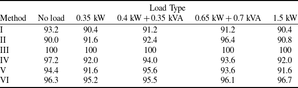
Under different loads, the above six different fault feature extraction methods are used to extract the features of I ef , and the fault dictionary is used for classification. Here, the simulation software is MATLAB; the main frequency of the computer is 2.9 GHz; the memory is 16 GB and the operating system is Windows 10. The specific diagnosis results are shown in Table 2.
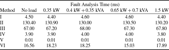
In addition, this paper calculates the fault analysis time (feature extraction and fault classification time) of each method under different loads, and the statistics of each time are only for a single sample. The specific statistical results are shown in Table 3. Among them, the PSO optimisation of method III and the training process of DBN of method VI are carried out offline, so their analysis time is not taken into account.
It can be seen from the results in Tables 2 and 3 that method II is better than method I under most load conditions. Compared with method II, method III (presented in this paper) has significantly improved the diagnostic accuracy, and after optimisation, the time consumption is reduced by nearly 50%. The methods IV, V and VI are fast in fault diagnosis. Among them, the diagnosis method based on FFT is the fastest and has high accuracy, which fully shows the effectiveness of this mainstream method in practical application. Method VI is based on FFT and DBN process. Its analysis speed is slightly slower, but the accuracy of fault diagnosis is improved.
4.0 Practical experiment validation
4.1 Experimental platform and signal acquisition
A three-stage AC synchronous generator is used as the experimental platform, and its structural composition, shown in Fig. 7, is coarsely consistent with its simulated counterpart. The platform is mainly composed of frequency converter, three-phase asynchronous speed-regulating motor (analog prime mover), civil three-stage brushless synchronous alternator, current Hall sensor, adjustable three-phase resistive-inductive load box and data acquisition system.
The platform uses a three-phase asynchronous speed-regulating motor to drive the generator for rotation. The excitation current generated is collected through a data acquisition system. Moreover, by manipulating a three-phase variable resistive-inductive load box, the generator can be adjusted to operate under different loads.
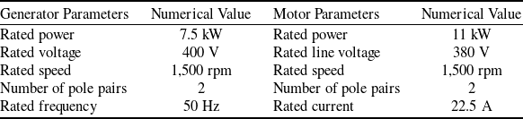
Additionally, to simulate various diode fault modes in the generator rotating rectifier, further modifications were designed and implemented. Initially, the brush and slip ring were used to securely mount the rotating rectifier onto the generator. Then, dual switches were installed for each rotating diode to simulate the diode’s open-circuit and short-circuit faults. Detailed parameters of generator and motor are shown in Table 4.
Diagnostic accuracy of different methods (%)

Fault analysis time of different methods

Main parameters of the experimental platform

Experimental platform components.

In applications, the excitation current I ef of the AC exciter is accessible. In our experiment, the HNC-25-LA Hall current sensor is selected as the current detection sensing element. This device enables electrical isolation between the primary measured current and the secondary output current, offering advantages such as fast response time and high measurement precision. It has a rated measurement current of 25 A and a coil turns ratio of 1:1,000, making it suitable for detecting low currents. The excitation current acquisition circuit is illustrated in Fig. 8. In this figure, R m represents the measurement resistance. The output current, passing through the measurement resistance R m , results in an output voltage U, which is proportional to the primary measured current I ef . The relationship between the voltage value U and excitation current I ef is as follows:
 \begin{align} U = \frac{1}{{1000}} \times {R_m} \times {I_{ef}} \end{align}
Schematic diagram of excitation current detection.

In this research, I ef is nearly 0.4 A. To accommodate the voltage input range of the AD converter and improve measurement resolution, R m is chosen to be 10 kΩ in this case.
The fault modes of rotating rectifier are consistent with the simulation experiment in the practical experiment. The excitation current I ef is collected under no load, 0.34 kW resistive load, 1.48 kW resistive load, 0.38 kW + 0.36 kVA resistive-inductive load, and 0.64 kW + 0.68 kVA resistive-inductive load at 10 kHz sampling frequency, and the sampling time is 100 ms, which means that the length of each sample is also 1,000 points. The excitation current waveforms for various fault modes under different loads are obtained, as shown in Fig. 9. For each load, 500 samples were collected, of which 250 were used as training samples, and the remaining 250 were utilised as diagnostic test samples.
The actual excitation current of each fault mode under different loads. (a) Excitation current of each fault mode under no-load. (b) Excitation current of each mode under resistive-inductive load (0.38 kW + 0.36 kVA).

The parameters of the civil three-stage brushless AC generator used in the practical experiment differ from those of the real aerospace generator. However, its internal structure and power generation principles are consistent with those of the aerospace generator. Therefore, despite some differences between the actual excitation current waveforms and the simulated excitation current waveforms (where the simulation model parameters are based on those of the real aerospace generator), the overall trends and variations are similar, which does not affect the validation of the algorithm.
4.2 Analysis of practical experiment results
The experimental analysis utilised data under different load conditions. The specific processing procedure is similar to that of the simulation experiment. Taking the no-load condition as an example, the Hilbert time-frequency spectra of the excitation current under different fault modes, after processing through HHT, are shown in Fig. 10.
Hilbert spectrum processed by HHT under different fault modes in practical experiment. (a) Healthy mode. (b) One-diode open fault. (c) Double-diode open fault. (d) One-diode short fault.

Comparison of instantaneous amplitude of each mode after decomposition under no-load. (a) After the decomposition of VHHT. (b) After the decomposition of PSO-VHHT.

The figure demonstrates that, in the practical experiment, the HHT method effectively captures the detailed variations in signal frequency and amplitude. After HHT processing, distinct differences in the instantaneous amplitude of the IMFs across different fault modes can be observed. However, due to inherent issues such as mode aliasing in EMD, significant fluctuations in the instantaneous amplitude occur, which may impact the accurate extraction of fault features.
The particle swarm optimisation algorithm is used to optimise the parameters of the secondary penalty factor and mode decomposition number of VHHT. The signal decomposition effects are compared by using VHHT algorithm and PSO-VHHT algorithm respectively. The Hilbert three-dimensional time spectrum comparison under different loads is shown in Figs 11 and 12. It can be observed that there are many instantaneous amplitude values in the one-diode short fault and one-diode open fault after VHHT decomposition, which can significantly affect the accuracy of subsequent marginal spectrum calculations, leading to substantial errors. In contrast, after PSO-VHHT decomposition, only a few instantaneous amplitude values remain, facilitating more accurate marginal spectrum calculations with reduced errors. The instantaneous amplitude values of the IMFs after PSO-VHHT decomposition remain stable, with no significant fluctuations observed. The distribution trends are consistent, and the magnitudes are nearly identical, thereby more accurately reflecting the signal variations under different fault modes, resulting in higher fault distinction compared to VHHT. This is because the decomposition effect of the VHHT algorithm is influenced by its mode decomposition number K and penalty factor α. A large K introduces redundant information, while a small K causes modal aliasing. Similarly, a high α narrows the bandwidth of each mode, causing distortion, whereas a low α introduces noise. K and α can be determined by experience, but a large error can probably be generated. By applying the PSO algorithm to these parameters, the optimal values of K and α can be found. Hence, the decomposition performance, particularly for clear marginal spectrum features extraction from AGRR excitation current signals, can be improved.
Diagnostic accuracy of different methods (%)

Comparison of instantaneous amplitude of each mode after decomposition under resistive-inductive load (0.38 kW + 0.36 kVA). (a) After the decomposition of VHHT. (b) After the decomposition of PSO-VHHT.

The fault feature extraction method used in the practical experiment is consistent with that in the simulation experiment. Method I: HHT is used for fault feature extraction; Method II: VHHT is used for fault feature extraction; Method III: PSO-VHHT is used for fault feature extraction; Method IV: EMD energy feature extraction method is used; Method V: FFT extracts the 1st, 2nd and 6th harmonic amplitudes as fault features; Method VI: FFT combined with DBN is used. The fault features obtained by these six methods are finally classified and diagnosed by fault dictionary. The diagnosis results of each method are shown in Table 5.
The fault analysis times for each method in the practical experiment were similarly collated for comparison, as shown in Table 6.
Fault analysis time of different methods

From the diagnostic results, it can be observed that compared to Methods I, II and IV, the proposed Method III (PSO-VHHT) effectively illustrates a very high diagnostic accuracy under different load conditions, indicating optimal decomposition performance. Additionally, this method reduces the diagnosis time by approximately 70% compared to Method II. Method V (FFT-based method) directly analyses the signal in the frequency domain without the need for complex preprocessing, making it the fastest among these methods. However, the diagnostic performance of these methods is inferior to the presented method. Method VI, which combines FFT-based analysis with DBN for feature extraction, also demonstrates good diagnostic performance, but it requires pre-training the network with complicated steps and a large number of samples. In conclusion, the results of the experiment are generally consistent with the simulations. Although the proposed method takes slightly longer diagnosis time compared to some existing methods, it significantly enhances feature extraction capability and improves overall fault diagnostic performance.
5.0 Conclusion
This study proposed a fault feature extraction method based on PSO-VHHT for aerospace generator rotating rectifiers. By integrating PSO algorithm with the VHHT, the method optimises VMD parameters, effectively addressing limitations such as mode aliasing and noise interference in traditional HHT and VHHT approaches. The PSO-VHHT method demonstrated superior signal decomposition precision, enhanced stability of instantaneous amplitude, and clearer fault features, resulting in a higher diagnostic accuracy across various load conditions. Additionally, the optimised method reduces diagnostic time compared to non-optimised VHHT, showcasing its potential capability of real-time fault detection in applications.
Future work will focus on improving the computational efficiency of PSO-VHHT to further enhance its real-time performance. Moreover, some advanced machine learning and pattern recognition models can be considered to combine with PSO-VHHT to enhance its capabilities of fault classification under complicated operational conditions, further increasing its utility in aerospace power systems.
Acknowledgements
This research was supported by Fundamental Research Funds for the Central Universities under Grant No. NS2021021 and Aeronautical Science Foundation of China under Grant No. 201933052001.
Competing interests
The authors declare that there is no conflict of interest in this work.