1. Introduction
Inviscid models are useful tools for prediction as well as cheaper alternatives to fully resolved simulations. Recently, the authors developed an inviscid model for viscous shear and boundary layers termed a vortex-entrainment sheet (DeVoria & Mohseni Reference DeVoria and Mohseni2019). This irregular surface is the superposition of a conventional vortex sheet having a discontinuity in the tangential velocity (i.e. harmonic potential) with an entrainment sheet having a discontinuity in the normal velocity (i.e. streamfunction). The former accounts for the vorticity in the real layer, while the latter accounts for its mass/momentum. It was proposed that the inclusion of entrainment in a model of this type could capture integral viscous-fluid phenomena, e.g. resistive drag, that are notably absent from conventional potential flow models.
In this paper, we further advocate and demonstrate the ability to represent viscous effects within our inviscid vortex-entrainment sheet model. For this express purpose we augment the set of self-similar solutions computed by Pullin (Reference Pullin1978) for the roll-up of conventional vortex sheets shedding from a sharp wedge. Pullin's seminal work has been highly influential in subsequent investigations that have marked continued advancements in the study of unsteady vortex dynamics. His paper will be liberally cited here and so it will henceforth be referred to simply as ‘Pullin’.
The forfeiture of the Navier–Stokes equations in favour of the inviscid model with an infinitely thin sheet bypasses the computational expense of resolving the detailed distributions of the velocity and vorticity across the viscous layer. However, we must inevitably incur this cost elsewhere, in part at least, if the viscous effects are to be captured in some integrated or even global sense. In short, we must supplement the inviscid model with boundary conditions that ideally contain the same level of information as those accompanying the Navier–Stokes equations. For example, the higher-order viscous equation allows one to impose the full velocity vector on the boundaries (with some mass conservation constraint for incompressible flows), which is not generally possible for the lower-order inviscid equation. One way of conveying more of this information to the inviscid model is to specify the normal velocity at the boundaries. In effect, this condition provides the zero-thickness sheet with the entrainment associated with the viscous layer that it replaces. The conventional vortex sheet is technically a special case of this, for which the entrainment is specified to be zero on all boundaries.
The vortex-entrainment sheet has a complex/vector strength and we introduce  $\nu =q/\gamma$ as the ‘strength ratio’ of the entrainment sheet strength
 $q$ to the vortex sheet strength
 $\gamma$. The entrainment is signed relative to the flow inside the sheet. Namely,
 $q>0$ means a net amount of mass/fluid enters the sheet, whereas
 $q<0$ means fluid emanates from the sheet. Pullin's solutions correspond to
 $\nu =0$ on all boundaries. In two dimensions, the velocity induced by the sheet at an arbitrary point
 $z$ in an otherwise unbounded domain can be expressed by the following generalized Birkhoff–Rott equation, i.e. Cauchy-type integral (DeVoria & Mohseni Reference DeVoria and Mohseni2019):
 \begin{equation} \frac{1}{2{\rm \pi} i}\int_{a(t)}^{b(t)}\frac{\gamma(s,t)-iq(s,t)}{z-z_s(s,t)}\,\textrm{d}s. \end{equation}
The integration is over the sheet whose position at time  $t$ is
 $z_s(s,t)$ with
 $s\in [a,b]$ as the arclength coordinate. In general, the dynamics of the sheet is governed by ‘surface equations’ resembling the Euler equations with a sheet density
 $\rho _s$ (mass per unit area) and with additional source terms representing the entrainment/flux of mass and momentum. Once the normal velocity boundary condition is specified, the outer potential flow problem can be solved and the mass flow into the vortex-entrainment sheets calculated. For the case of a solid body geometry, the sheet fixed to its surface represents the boundary layers and their entrainment. Here, the additional momentum terms include the stress jump across the sheet. As such, the stress on the surface side can be evaluated and integrated to give an estimate of the force on the body, which includes a viscous effect owing to the entrainment. For more details, the interested reader is referred to DeVoria & Mohseni (Reference DeVoria and Mohseni2019).
Since our aim here is to obtain self-similar solutions to the outer problem, we bypass the surface equations by searching for solutions that are governed by (1.1) when  $z\rightarrow z_s$. Dynamically, this means the pressure jump across the sheet (supported by
 $\rho _s\neq 0$) is such that the sheet moves with the average of the discontinuous velocities on each side of the sheet, namely the principal value. Of course, when the sheet contains no mass and has zero entrainment, the equation of motion reduces to the conventional kinematic Birkhoff–Rott equation for a massless vortex sheet.
The Lagrangian formulation used by Rott (Reference Rott1956) and Birkhoff (Reference Birkhoff1962) substitutes the arclength  $s$ (or some scalar parameter) for the amount of circulation
 $\varGamma (s,t)$, as measured from a reference point on the sheet, via the relationship
 $\gamma =\partial \varGamma /\partial s$. This approach has been used by many authors in the study of vortex sheet dynamics (e.g. Moore Reference Moore1979; Krasny Reference Krasny1987; Jones Reference Jones2003) as it has several utilities stemming from the transformal invariance of the circulation. Analytically, this requires that
 $\varGamma$ is a monotonic function of the Lagrangian parameter with an injective inverse. Physically, this represents the continual generation of vorticity of one sign, which here leads to a power-law growth (a functionality typical to similarity solutions) of total circulation in the sheet.
For the vortex-entrainment sheet we now employ the strength ratio  $\nu (s,t)$ in order to use the Lagrangian formulation. As such, (1.1) becomes
 \begin{equation} \frac{1}{2{\rm \pi} i}\int_0^{\varGamma_s(t)}\frac{1-i\nu(\varGamma^{\prime},t)}{z -z_s(\varGamma^{\prime},t)}\,\textrm{d}\varGamma^{\prime}, \end{equation}
with  $\varGamma _s(t)$ as the total amount of circulation in the sheet at time
 $t$. In § 2 we apply the above framework to a generalized problem for the case of starting flow over an infinite wedge with separation, which is then simplified to a self-similar problem in § 3. Several sets of numerical solutions are presented and discussed in §§ 4 and 5, with comparison to experiment in § 4.3. The novel objective of the paper is to draw plausible physical connections between entrainment in the inviscid sheet model and viscous effects.
2. General problem formulation
The attached flow around the wedge is given by a known complex potential  $W_o(z,t)$. This flow is singular at the wedge apex and is regularized by allowing separation at the sharp edge to form the free sheet. Formally, the potential
 $W_o(z,t)$ is obtained as a transformation from a virtual domain with complex variable
 $\zeta$, where
 $W_o(\zeta ,t)=\sum _{k=-\infty }^{\infty }A_k(t)\zeta ^k$ is a Laurent series expansion about
 $\zeta =0$ and, in general, the coefficients are complex:
 $A_k(t)\in \mathbb {C}$ (e.g. see Batchelor Reference Batchelor1967, pp. 128, 410). The series that is convergent near
 $|\zeta |=0$ has
 $A_k=0$ for
 $k<0$. For the wedge of internal angle
 $\beta {\rm \pi}(0<\beta <1)$ and bisector along the real axis in the physical domain, the transformation
 $\zeta =z^n$ with
 $n=1/(2-\beta )$ maps the wedge faces to the imaginary axis
 $\zeta =iy^*$ (see figure 1). We then have
 \begin{equation} W_o(z,t)=A_0(t)+A_1(t)z^n+A_2(t)z^{2n}+\cdots+A_k(t)z^{kn}+\cdots. \end{equation}
Since  $\frac {1}{2} < n<1$, then in the limit
 $z\rightarrow 0$ the dominating, singular term in the velocity expression,
 $\textrm {d}W_o/\textrm {d}z$, of this attached flow is the
 $k=1$ term. However, we note that retention of other terms in the series (including
 $k<0$ ones) offers a more generalized description of the flow and allows more topologically rich features to occur. Such possibilities are beyond the scope of the current paper, however, and are reserved for future work. Moving on, we may also take
 $A_0=0$ or, equivalently, define
 $W_o^\prime =W_o-A_0$ without affecting the velocity. Hence, for
 $|z|\ll 1$ the complex potential is taken as
 $W_o=A_1(t)z^n$ and represents the mapping of an instantaneously uniform flow in the virtual domain to the physical domain. Pullin considered the vertical component of this uniform flow so that
 $A_1(t)$ was purely imaginary. Here, we consider an arbitrarily oriented stream and write
 \begin{equation} A_1(t)=U_n(t)-iU_t(t)\rightarrow \frac{\textrm{d}W_o}{\textrm{d}z}=nz^{n-1}\{U_n-iU_t\}. \end{equation}
Going forward,  $U_t$ and
 $U_n$ will be referred to as ‘virtual velocities’ having dimensions
 $[L]^{2-n}\cdot [T]^{-1}$, which when multiplied by the mapping derivative
 $\textrm {d}\zeta /\textrm {d}z=nz^{n-1}$ yield a physical velocity.
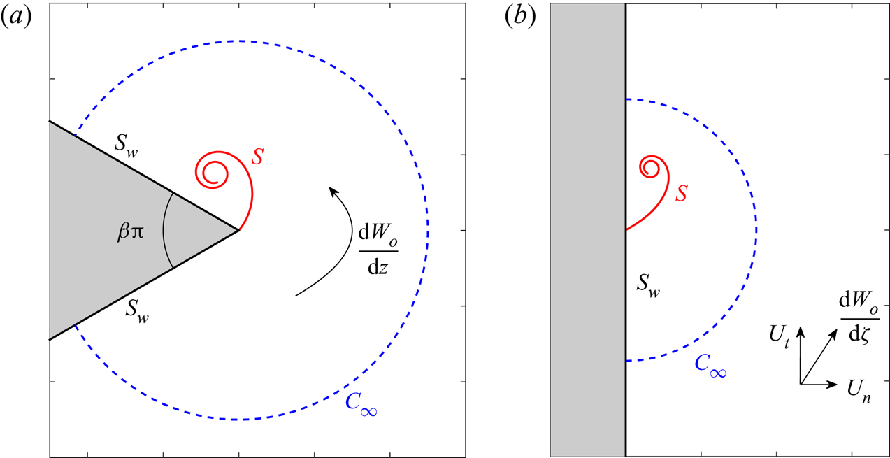
Problem geometry and definitions used in this paper. The wedge angle is  $\beta {\rm \pi}$. The analytic fluid domain is given by the simply connected region bounded by the freely shed sheet
 $S$, the wedge surface sheet
 $S_w$ and the arc
 $C_\infty$ at infinity. Mass entrainment may occur on the vortex-entrainment sheets
 $S$ and
 $S_w$, whereas
 $C_\infty$ is an ordinary curve across which fluid simply passes. (a) Physical
 $z$-plane with
 $\textrm {d}W_o/\textrm {d}z$ as the attached driving flow. (b) Virtual
 $\zeta$-plane defined by the mapping
 $\zeta =z^n$ with
 $\textrm {d}W_o/\textrm {d}\zeta =U_n-iU_t$ as the uniform virtual velocity whose components are tangential and normal to the mapped wedge boundary.

By superposition, the external flow is combined with the contribution from the free sheet,  $S$, and the sheet representing the wedge surface,
 $S_w$, to give the total velocity
 $\textrm {d}W/\textrm {d}z$. To have a well-posed problem with a unique solution, we must specify the normal velocity
 $u_n$ on all boundaries, which includes a contour
 $C_\infty$ at infinity that intersects the wedge surfaces there (recall figure 1). Stated differently, we must give the entrainment into or flux across each of these boundaries. Note that
 $C_\infty$ is an ordinary curve with no dynamical significance and is not the location of a discontinuity.
For the free sheet it suffices to give its strength ratio  $\nu$. For the wedge surface the boundary condition is typically assumed to be one of no through flow. However, the
 $S_w$ sheet represents the boundary layers on the wedge and thus any entrainment associated with those layers is given by a non-zero normal velocity. The Cauchy integral for the velocity field is a boundary integral formulation of the solution to the Laplace equation (with kernel appropriate to the geometry) and so the flow at infinity is automatically ensured to have the correct behaviour.
Our end goal of obtaining self-similar solutions is eased if we can eliminate the specification of as many functions and parameters as possible. Our approach to this problem is the method of images. This reduces the degree of freedom from a doubly infinite set to a singly infinite one by providing a relation for the velocity contribution from the wall sheet in terms of the parameters defining the free sheet. In other words, specifying either  $u_n$ on the wall or
 $\nu$ on the free sheet will, in principle, determine the other.
The image system is not unique, however. The parameters defining a given sheet are its position and strength, both of which are complex quantities. To allow for some generality, we define the image system with four degrees of freedom as follows. The position in the virtual domain,  $z_i^n$, is taken to be a scaling and rotation of the standard ‘mirror image’:
 $z_i^n=-\overline {A^nz_s^n}$, where
 $A=M\,\textrm {e}^{\textrm {i}\varTheta }$ is to be given; an overbar denotes the complex conjugate. Next, we write the strength of the image sheet as
 $-(c_\gamma \gamma -ic_q q)$, where
 $c_\gamma$ and
 $c_q$ are two real constants also to be given;
 $c_\gamma =1$ corresponds to the negative of the vortex sheet strength as is usually used. For convenience we define
 $\chi =(1-i\nu )$ and
 $\chi _i=-(c_\gamma -ic_q\nu )$, and so the expression for the velocity field becomes
 \begin{equation} \frac{\textrm{d}W}{\textrm{d}z}=nz^{n-1}\left\{(U_n-iU_t)+\frac{1}{2{\rm \pi} i}\int_0^{\varGamma_s} \left[\frac{\chi^\prime}{z^n-z_s^{\prime n}}+\frac{\chi_i^\prime}{z^n-z_i^{\prime n}} \right]\,\textrm{d}\varGamma^{\prime}\right\}, \end{equation}
where  $\chi ^\prime =\chi (\varGamma ^\prime )$ and so on, and explicit time dependence has been dropped for clarity. If
 $u_t$ and
 $u_n$ are the tangential and normal physical velocity components on the wedge faces, where
 ${arg}\{z^n\}=n\theta =\pm {\rm \pi}/2$, then the velocity/boundary condition there becomes
 \begin{equation} u_t-iu_n=\pm nr^{n-1}\{(U_t+u_t^*)+i(U_n+u_n^*)\}, \end{equation}
where  $u_t^*$ and
 $u_n^*$ are the corresponding tangential and normal virtual velocities (i.e. having units
 $[L]^{2-n}\cdot [T]^{-1}$) on the wedge. The removal of the singularity in each physical velocity component at
 $r=|z|=0$ requires that
 \begin{equation} 0+i0=(U_t+iU_n)-\frac{1}{2{\rm \pi} }\int_0^{\varGamma_s}\left[\frac{\chi}{z_s^{n}}+ \frac{\chi_i}{z_i^{n}}\right]\,\textrm{d}\varGamma. \end{equation}
This is a complex/vector Kutta condition so that we have an additional condition to impose (the imaginary part) as compared to the baseline case of zero entrainment everywhere that was treated by Pullin. Physically, these conditions determine the total circulation  $\varGamma _s$ and net entrainment rate
 $Q_s$ in the free sheet.
One usually thinks of specifying the normal velocity  $u_n$ on the wedge surface as the boundary condition, which will close the problem. However, this leads to an inverse problem for
 $\nu (\varGamma ,t)$ that is ill conditioned in the same way as Fredholm integrals of the first kind. Alternatively, if
 $\nu$ is known, then the problem becomes well posed and the solution unique. We need only give a ‘normalized’ distribution of
 $\nu$ since the imaginary part of the vector Kutta condition is sufficient to determine
 $Q_s=\int \nu \,\textrm {d}\varGamma$, which is a scalar quantity. We note that the conventional vortex sheet is a special case of this approach, whereby one imposes the strength ratio to be identically zero on the sheet.
In summary, since we are prescribing the (normalized) strength ratio  $\nu$ of the free sheet, then for the general case we have a seven-parameter solution family:
 $n$ for the wedge geometry,
 $U_t$ and
 $U_n$ specifying the driving flow, and
 $c_\gamma$,
 $c_q$,
 $M$ and
 $\varTheta$ defining the wall normal boundary condition (i.e. the image system). The unknowns to be obtained from the solution are the sheet position
 $z_s$, its total circulation
 $\varGamma _s$, and its net entrainment rate
 $Q_s$.
2.1. The boundary condition at infinity
The expansion in (2.1) was introduced in the context of a convergent series near the apex,  $r\rightarrow 0$. However, the domain in our mathematical problem is radially infinite and we may consider the behaviour at infinity through a similar series, although it need not be convergent insofar as
 $W(z)$ is concerned. This multi-pole expansion combines fundamental solutions of the two-dimensional Laplace equation (known as circular harmonics) and generally contains a logarithmic term. From the
 $r\rightarrow \infty$ limit on (2.3) it can be shown that this logarithmic term corresponds to the contribution
 $W_s$ from the free sheet (and its image). Specifically, the total complex potential approaches
 \begin{equation} W = W_o+W_s = z^n(U_n-iU_t)+\frac{1}{2{\rm \pi} i}[(1-c_\gamma) \varGamma_s-i(1-c_q)Q_s]\log z^n. \end{equation}
The velocity induced by the sheet at infinity is therefore equivalent to that of a point singularity of strength  $n[(1-c_\gamma )\varGamma _s-i(1-c_q)Q_s]$ located at the apex. However, this velocity decays faster than the driving flow:
 $z^{-1}$ vs.
 $z^{-(1-n)}$. Hence, by (2.4) the normal velocity on the wedge surfaces at infinity must approach
 $u_n=\mp nr^{n-1}U_n$.
The total circulation around and the total mass flux across all boundaries must be zero; these requirements are sometimes called compatibility conditions. Since  $W_o$ is itself a solution to the Laplace equation, then it independently satisfies these constraints. Therefore, we may reduce the compatibility conditions as applied to just the flow induced by the sheet and its image
 \begin{equation} \varGamma_s+\varGamma_w=\varGamma_\infty,\quad Q_s+Q_w=Q_\infty, \end{equation}
where  $Q_\infty$ is the net flux across
 $C_\infty$ due to the sheet-induced flow there and likewise for
 $Q_w$ as the net entrainment associated with the wedge
 $S_w$; similar definitions apply to
 $\varGamma _\infty$ and
 $\varGamma _w$ as the corresponding circulations on these boundaries. Integrating the expression for
 $\textrm {d}W_s/\textrm {d}z$ along the arc
 $C_\infty$ we obtain the following additional relations:
 \begin{equation} \varGamma_\infty =\tfrac{1}{2}(1-c_\gamma)\varGamma_s,\quad Q_\infty =\tfrac{1}{2}(1-c_q)Q_s. \end{equation}
We immediately see how the choices of  $c_\gamma$ and
 $c_q$ affect the flow at infinity. By substitution into (2.7a,b), there are similar consequences for the wall quantities
 $\varGamma _w$ and
 $Q_w$.
Before continuing, we will find the following quantity useful in non-dimensionalizing the problem. For any sheet, segment of sheet, or arc we define
 \begin{equation} \varGamma-iQ=\varGamma(1-i\tilde{\nu}), \end{equation}
so that  $\tilde {\nu }=Q/\varGamma$ is the ratio of the flux to the circulation associated with the curve. For a vortex-entrainment sheet with
 $\varGamma -iQ=\int (1-i\nu )\,\textrm {d}\varGamma$, then
 $\tilde {\nu }$ is the average of
 $\nu (\varGamma )$ on the curve, e.g.
 $\tilde {\nu }_s=Q_s/\varGamma _s$ for the free sheet. For an arc that is not the location of a discontinuity, then
 $\varGamma -iQ=\int (u_t+iu_n)\,\textrm {d}l$ as usual. In particular, the attached driving flow,
 $\textrm {d}W_o/\textrm {d}z$, defines
 $\tilde {\nu }_o=Q_o/\varGamma _o=-U_n/U_t$ on the arc
 $C_\infty$ at infinity.
3. The self-similar problem
Here, we identify the restrictions that are required for a solution to be self-similar. First, the similarity form and variable are defined as
 \begin{equation} z_s(\varGamma,t)=L(t)\omega(\lambda),\quad \lambda=1-\frac{\varGamma}{JG(t)}, \end{equation}
where  $L(t)$ is a time-dependent physical length scale,
 $\omega (\lambda )=\xi (\lambda )+i\eta (\lambda )$ is the self-similar shape function with similarity variable
 $\lambda$, and
 $G(t)$ is the temporal growth of
 $\varGamma$ with
 $J$ as a non-dimensional constant corresponding to the total circulation. Note that
 $\varGamma$ is defined as the circulation between a point
 $z_s(\varGamma ,t)$ and the rolled-up tip of the sheet where
 $\lambda =1$. At the apex
 $\lambda =0$ and so
 $\varGamma _s=JG$.
Writing  $U_t(t)=\dot {Y}(t)$ we first find that
 $C_o=(L^{1-n}\dot {L})/\dot {Y}$ must be a non-dimensional constant; recall that
 $U_t=\dot {Y}$ has units
 $[L]^{2-n}\cdot [T]^{-1}$. The next constraint for the solution to be self-similar is
 \begin{equation} Q_P=\frac{\dot{G}/G}{\dot{L}/L}=n+(2-n)\frac{Y\ddot{Y}}{\dot{Y}^2}=\textrm{const.} \end{equation}
The symbol  $Q_P$ is not to be confused with an entrainment rate; the subscript ‘
 $P$’ indicates ‘Pullin’ who used
 $Q$ with no subscript for this term. Hence, the (logarithmic) growth of the circulation must be proportional to that of the sheet size. The further constraint
 $Y\ddot {Y}\propto \dot {Y}^2$ implies that the work required to move the wedge with ‘virtual velocity’
 $\dot {Y}$ is proportional to its kinetic energy. The power-law form
 $\dot {Y}(t)=a(t+b)^m$ satisfies this condition irrespective of the values
 $a$ and
 $b$, and gives
 $Q_P=(n+2m)/(1+m)$. The exponential law
 $\dot {Y}(t)=a\textrm {e}^{bt}$ is also valid and represents the
 $m\rightarrow \infty$ limit of the algebraic form. We adopt the former choice with
 $b=0$ (as did Pullin), and the length scale then becomes
 \begin{equation} L(t) = [C(at^m)t]^{{1}/({2-n})}, \end{equation}
with  $C=C_o(2-n)/(1+m)$ as another non-dimensional constant. Next, the differential circulation is
 \begin{equation} \frac{-\textrm{d}\varGamma}{L^n\dot{Y}}=\frac{JG(t)\,\textrm{d}\lambda}{(L^2/t)/C}, \end{equation}
which gives  $G(t)=(L^2/t)/C=(L\dot {L})/C_o$. Following Pullin, the constant
 $C_o$ is taken as
 $C_o=(1-n)$ and so (2.3) finally becomes the following integro-differential equation:
 \begin{gather} (1-n)\left[\bar{\omega}+Q_P(1-\lambda)\frac{\textrm{d}\bar{\omega}}{\textrm{d}\lambda}\right] =\frac{\textrm{d}\varOmega}{\textrm{d}\omega}, \end{gather}
 \begin{gather}\frac{\textrm{d}\varOmega}{\textrm{d}\omega}=n\omega^{n-1}\left\{-i(1-i\tilde{\nu}_o)+\frac{J}{2{\rm \pi} i}\int_0^1\left[\frac{\chi^\prime}{\omega^n-\omega^{\prime n}}+\frac{\chi_i^\prime}{\omega^n-\omega_i^{\prime n}}\right]\,\textrm{d}\lambda^{\prime}\right\}, \end{gather}
where  $\omega _i^n=-\overline {A^n\omega ^n}$ is the image sheet,
 $\varOmega (\omega )$ is the non-dimensional complex potential and again
 $\tilde {\nu }_o=Q_o/\varGamma _o=-U_n/U_t$. The vector Kutta condition in (2.5) takes the following non-dimensional form:
 \begin{equation} 0=(1-i\tilde{\nu}_o)-\frac{J}{2{\rm \pi} }\int_0^1\left[\frac{\chi}{\omega^{n}}+ \frac{\chi_i}{\omega_i^{n}}\right]\,\textrm{d}\lambda. \end{equation}
The quantity  $\tilde {\nu }_o$ may, in general, be a function of time. This is permissible because the Laplace equation is elliptic and all other time dependency in (3.5) has been removed. Hence, the spatial problem can be solved with the instantaneous value. In this way, a separate implicit time dependence can exist in the solution as
 $z_s(t)=L(t)\omega (\lambda;\tilde {\nu }_o(t))$, which allows the actual sheet shape to evolve in a more complex way. The same is also true for the other input parameters in the problem (see figure 5 and corresponding discussion in § 4.3).
For the non-dimensional, self-similar problem the driving flow is now specified by  $m$ and
 $\tilde {\nu }_o$, while the parameters describing the wedge geometry and the image system remain the same. The normal boundary condition on the wedge at infinity is
 $u_n=\pm nr^{n-1}\tilde {\nu }_o$. The unknowns to be found are the sheet position
 $\omega$, its total circulation
 $J$ and its average strength ratio
 $\tilde {\nu }_s=Q_s/\varGamma _s$.
3.1. Approximation of the core region
Due to the tightly wound turns within the rolled-up spiral, it is not very sensible to fully resolve (3.5) in this region. Instead, it is common to replace the core region with an isolated point singularity that connects to the severed sheet via a branch cut. The motion of this singular point is determined by imposing a ‘zero-net-force’ condition on the branch cut system, representing the conservation of linear momentum. We adopt the usual model that balances a pressure jump force acting on the cut with a Joukowski force acting on the point (Brown & Michael Reference Brown and Michael1954; Rott Reference Rott1956). Here, the Joukowski force will have a conjugate contribution from the entrainment constituent.
First, by (2.9) the complex strength of the singular core point is  $\varGamma _c(1-i\tilde {\nu }_c$), where
 $\tilde {\nu }_c$ is the average of the strength ratio in the core region. In terms of the similarity variables the non-dimensional strength is
 $J(1-\lambda _c)(1-i\tilde {\nu }_c)$ with
 $\lambda _c$ as the value of
 $\lambda$ where the cut has been made. Likewise, the zero-force condition serving as the governing equation for the point is
 \begin{equation} \left.\frac{\textrm{d}\varOmega}{\textrm{d}\omega}\right|_{\omega_c}= (1-n)\left[\bar{\omega}_c+Q_P\left(\frac{\bar{\omega}_c- \bar{\omega}_s}{1-i\tilde{\nu}_c}\right)\right], \end{equation}
where  $\omega _c$ and
 $\omega _s$ are the locations of the singular core point and the end of the severed sheet, respectively. The above was used by Pullin with
 $\tilde {\nu }_c=0$, although he did not explicitly give this equation.
3.2. Asymptotic solution near the apex
By analytically enforcing the Kutta condition Pullin obtained the asymptotic solution for  $\omega (\lambda )$ very near the wedge apex (
 $\lambda \rightarrow 0$). He showed that the vortex sheet must shed tangential to the windward wedge face, while the flow on the leeward face is consequently stagnated at the apex and thus has no contribution to the free sheet. The details of the analogous process for the vortex-entrainment sheet are provided in appendix A and here we simply state the results. Also, we take
 $U_t>0$ going forward.
The vortex-entrainment sheet has a continuously variable shedding angle  $\theta _a$ at the apex. Defining
 $c_a=c_q\nu _a/c_\gamma$ where
 $\nu _a=\nu (0)$ is the strength ratio at the apex, then
 $\theta _a$ is given by
 \begin{equation} \theta_a=\frac{1}{2}\left[\arccos\left(\frac{M\cos\beta{\rm \pi} }{c_\gamma \sqrt{1+c_a^2}}\right)+\arctan(c_a)-\varTheta\right]. \end{equation}
The limiting (non-dimensional) velocities on the leeward ( $+$ superscript) and windward (
 $-$ superscript) sides of the sheet at the apex are
 \begin{equation} (u_{t,a}^{\pm}-iu_{n,a}^{\pm})=\frac{JP}{2|K|}\left[1\mp\frac{(1-i\nu_a)}{P}\right], \end{equation}
with  $u_{t,a}$ and
 $u_{n,a}$ being the tangential and normal components relative to the sheet, and
 $P$ and
 $K$ are functions of
 $\nu _a$ and
 $\beta$, as well as the parameters describing the image system as defined in appendix A. The definitions of the vortex and entrainment sheet strengths are
 $\gamma = u_{t}^{-}-u_{t}^{+}$ and
 $q = u_{n}^{-}-u_{n}^{+}$, and it can be verified from (3.9) that the strength ratio at the apex satisfies
 $\nu _a=q_a/\gamma _a$ as required. Due to the entrainment the flow is no longer stagnated on the leeward side, but instead interacts with that on the windward side to contribute to the forming free sheet.
In the following two sections we will consider certain solutions to the problem outlined above. In § 4, entrainment is limited to the wedge surfaces  $S_w$ whereas the free sheet
 $S$ is a conventional vortex sheet. In § 5, both
 $S_w$ and
 $S$ will have non-zero entrainment.
4. Wedge-surface entrainment
In this section we present solutions to (3.5) and (3.6). The numerical approach is essentially the same as Pullin's and inclusion of entrainment does not present any new difficulties in this regard. Hence, the finite-difference forms of the equations have been relegated to appendix B. The current study is limited to the impulsive start with  $m=0$. Pullin showed that
 $m>0$ results in a more compact core region with increased ellipticity and a larger fraction of the total circulation in the outer turns of the sheet (i.e. increasingly stronger vorticity is generated at the apex by the acceleration). Here, the presence of entrainment will be limited to the wedge or wall surfaces; entrainment on the free sheet will be discussed in § 5.
4.1. Validation and large wedge angle results
As validation, we first reproduced Pullin's results for zero entrainment everywhere on all boundaries:  $\nu (\lambda )\equiv 0$ and
 $\tilde {\nu }_o=0$. This corresponds to an image system with
 $c_\gamma =1$,
 $M=1$ and
 $\varTheta =0$ (
 $c_q$ is irrelevant since
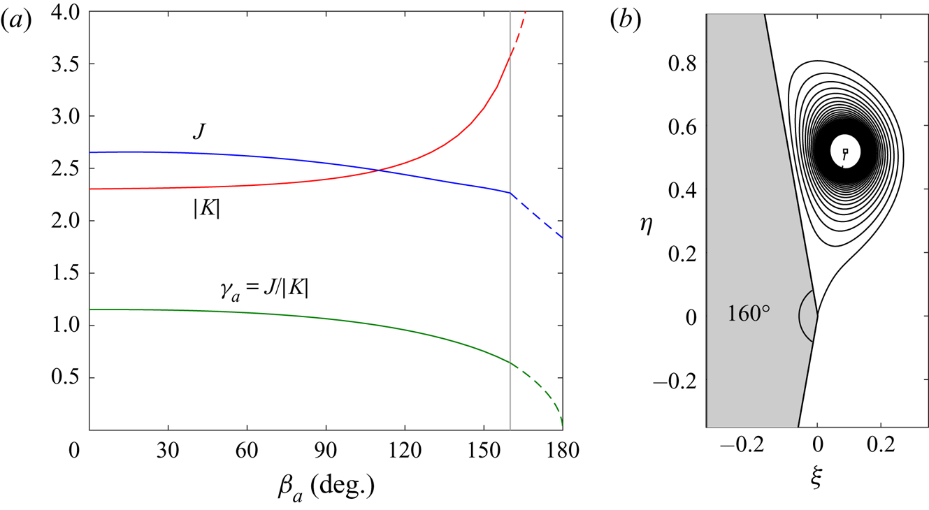
 $\nu =0$). He was limited by computer storage and thus had a coarser angular resolution of points on the sheet, most particularly near the apex. Using similar spacing we were able to quantitatively obtain his results (his figures 11–13). With the benefit of modern computing, a finer resolution showed that the solutions converge to slightly different values, but which vary only by a few per cent. Some relevant quantities from these latter results are shown in figure 2(a). Specifically, the total circulation
 $J$ and the vortex sheet strength at the apex
 $\gamma _a$ are plotted as functions of the wedge apex angle
 $\beta _a$ in degrees. The two quantities are related as
 $\gamma _a=J/|K|$, where
 $K$ is a complex proportionality constant in the asymptotic solution
 $\omega = K\lambda$ near the apex (see appendix A) and is also plotted.
Selected numerical results for the baseline case of zero entrainment. (a) Variation of non-dimensional solution parameters with wedge angle  $\beta _a$. The vertical line marks
 $\beta _a=160^{\circ }$ above which numerical solutions were not converged; the dashed lines are approximations for
 $\beta _a>160^{\circ }$ (see text). (b) The solution for
 $\beta _a=160^{\circ }$ with 36 resolved turns. The isolated core point vortex (white square) contains 25 % of the total circulation.

Similar to Pullin, we also were not able to obtain converged solutions for  $\beta _a > 160^{\circ }$. This is because the numerical method relies on specification of a unique angular coordinate
 $\vartheta$ for each point on the sheet as measured from the datum line connecting the core point and the wedge apex. The solution for
 $\beta _a=160^{\circ }$ is plotted in figure 2(b) and reveals that the datum for
 $\vartheta$ is nearly in line with the tangent direction of the lower wedge face, along which the sheet must shed. For larger wedge angles the
 $\vartheta$ of sheet positions near the apex were no longer unique.
Nevertheless, we may infer the behaviour for  $\beta _a\rightarrow 180^{\circ }$ (or
 $\beta \rightarrow 1$) by utilizing the asymptotic solution. In this limit the outer flow approaches a uniform flow. However, the boundary condition at the apex (i.e. the Kutta condition) ensures that a non-zero amount of circulation
 $J$ will be shed. Rewriting the expressions for
 $\gamma _a$ and
 $|K|$ from appendix A in terms of
 $\beta$, we obtain the following relations for large wedge angles:
 \begin{equation} \gamma_a=c\sqrt{1-\beta}, \quad J=\frac{c^2(2-\beta)}{2Q_P}, \quad |K|=\frac{c(2-\beta)}{2Q_P}\frac{1}{\sqrt{1-\beta}}. \end{equation}
Here,  $c\approx 1.93$ was determined by matching
 $\gamma _a$ to the
 $\beta _a=160^{\circ }$ solution. These equations are plotted in figure 2(a) as dashed lines. The approximations are quite good for
 $\gamma _a$ and
 $|K|$, appearing continuously differentiable. While there is a ‘kink’ in the trend for
 $J$, the values are reasonable. As
 $\beta \rightarrow 1$ the vortex sheet strength becomes very weak, with
 $\gamma _a\rightarrow 0$ at the apex, and so the vorticity of total circulation
 $J\rightarrow 1.86$ becomes more concentrated in the spiral core.
Next, we investigate cases of non-zero entrainment. Our initial interest is in the qualitative effects of entrainment for a given solution. Since the rolled-up spiral shape is topologically similar for all wedge angles (see Pullin's figure 9), we will henceforth focus on the specific wedge angle of  $\beta _a=60^{\circ }$ corresponding to
 $n=0.6$.
4.2. Some new vortex sheet solutions
As discussed in § 2, a unique solution for a given  $\tilde {\nu }_o=Q_o/\varGamma _o$ requires that we specify the functional distribution of the strength ratio
 $\nu (\lambda )$ along the free sheet. This clearly represents a considerable amount of freedom, in fact, an infinite amount. With this in mind, we recall that the conventional vortex sheet, which has proven to be a valuable model, is a special case having
 $\nu \equiv 0$ on the sheet. For our current problem there are actually additional vortex sheet solutions other than those found by Pullin and we now consider these possibilities. There are two main physical implications, the first being the usual inviscid fluid assumption such that vorticity is not diffused from the free sheet. Consequently, any entrainment must occur on the wall-bound sheets and represents the effect of the no-slip condition on the solid wedge surfaces in a viscous fluid. There is no intuitive meaning to the image system other than when it satisfies a desired boundary condition (e.g. the wedge is a streamline or zero entrainment at infinity). To this end, we endeavour to stray as little as possible from Pullin's situation by taking
 $c_\gamma =1$ and
 $\tilde {\nu }_o=0$ (again
 $c_q$ is irrelevant here). Since
 $\nu \equiv 0$, then we have technically imposed
 $\tilde {\nu }_s=0$, or
 $Q_s=0$ rather, and so a degree of freedom is lost. This means that for each
 $M$ there is a unique value of
 $\varTheta$, which is now to be found as part of the solution rather than given.
From (2.8a,b) we find that  $\varGamma _\infty =0$ and
 $Q_\infty =0$, and subsequently from (2.7a,b) that
 $\varGamma _s=-\varGamma _w$ and
 $Q_w=0$. Recall that these circulations and entrainments are those due to the velocity induced by just the free sheet (i.e. excluding the driving flow). Therefore, the circulation in the free sheet will be equal and opposite to that which it induces on the wedge. While the net entrainment from the walls is zero, there is a non-zero local flux at any given point; since
 $\tilde {\nu }_o=0$ the driving flow, being everywhere tangent to the wedge, has no contribution to this local entrainment.
By the requirements in appendix A, there is a finite range  $0<M<M_{max}$, which here is limited by
 $M_{max}=1/|\cos \beta {\rm \pi}|=2$. In the numerical set-up we varied
 $M$ within this range and the scheme solved for the corresponding unique
 $\varTheta$ value. For comparison, another related set of solutions is obtained in a similar fashion. Namely, the effect of a non-zero flux at infinity due to the driving flow is included by allowing
 $Q_o\neq 0$, this flow now having a component normal to the wedge boundary. Equivalently,
 $\tilde {\nu }_o\neq 0$ and its unique value corresponding to a specified
 $M$ is now the quantity to be obtained from the solution, thus replacing
 $\varTheta$ which is returned to the fixed value
 $\varTheta =0$ of the baseline case. Both solution sets will now be discussed.
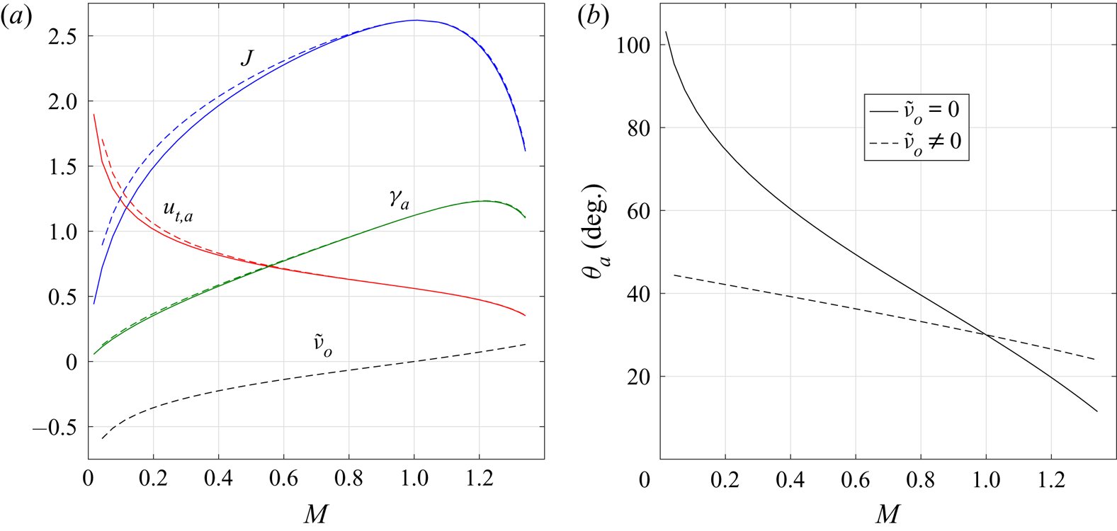
Figure 3(a) plots  $J$,
 $\gamma _a$, and the shedding velocity at the apex
 $u_{t,a}$, each as a function of
 $M$; above
 $M\approx 1.35$ the system became very ‘stiff’ and solutions no longer converged. The results are remarkably similar, despite different boundary conditions at infinity, being essentially identical for
 $M>1$ and only a slight diverging for
 $M<1$. For the cases with
 $\tilde {\nu }_o\neq 0$, this quantity is also plotted and reveals that
 $(M-1)$ and
 $\tilde {\nu }_o$ have the same sign. This allows us to infer that the effect of the image system for the
 $\tilde {\nu }_o=0$ cases is to nearly preserve the plotted quantities. Moreover, recalling that
 $\tilde {\nu }_o=-U_n/U_t$, we can then interpret this quantity as a measure of a ‘streamwise’ flow component, with
 $\tilde {\nu }_o<0$ meaning flow away from the wall and
 $\tilde {\nu }_o>0$ toward the wall. The direction of the flow relative to the apex then explains why the total circulation
 $J$ decreases from the baseline for all cases, as well as the simultaneous increase/decrease of
 $\gamma _a$ with
 $\tilde {\nu }_o$. However, the solutions display significant differences in the sheet position. For example, figure 3(b) plots the shedding angle
 $\theta _a$ vs.
 $M$ for the two sets. While
 $\theta _a$ increases/decreases away from the wedge tangent (
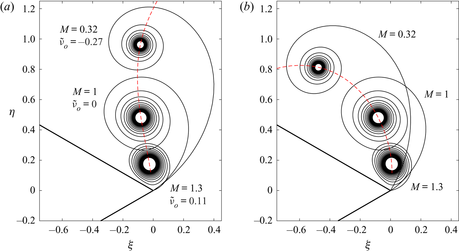
 $\theta _a=\beta _a/2=30^{\circ }$) of the baseline case for both sets, the corresponding rates are considerably different. The differences are best observed from the sheet positions as shown in figure 4. Also shown is the trajectory of the isolated core point. When the ‘streamwise’ flow is away from the wall (
 $\tilde {\nu }_o<0$) the core is convected downstream thus elongating the arclength of the outermost turn that connects to the apex. Conversely, when this flow is toward the wall (
 $\tilde {\nu }_o>0$), the overall sheet size shrinks toward the apex with the outer turns becoming much closer. When
 $\tilde {\nu }_o=0$ the same features occur, but the core trajectory encroaches further along the upper wedge surface, as expected from the dominant tangential flow around the apex.
Results for two solution sets with a conventional vortex sheet  $S$ in the fluid, but non-zero local entrainment on
 $S_w$ the wedge surfaces.
 $\tilde {\nu }_o=0$ (solid lines);
 $\tilde {\nu }_o\neq 0$ (dashed lines), where
 $\tilde {\nu }_o=Q_o/\varGamma _o$ is the boundary condition at infinity.
 $M$ is the scaling factor in the image system. (a) Total circulation
 $J$, vortex sheet strength
 $\gamma _a$ and shedding velocity
 $u_{t,a}$ at the apex. (b) The shedding angle
 $\theta _a$. The baseline case of Pullin is
 $M=1$ with
 $\theta _a=\beta _a/2=30^{\circ }$.

Sheet shapes for the two solution sets described in figure 3 with different boundary conditions at infinity  $\tilde {\nu }_o$ as labelled. The dashed red line is the trajectory of the core point as
 $M$, the image system scaling, is continuously varied.
 $M=1$ is the baseline case of Pullin. (a)
 $\tilde {\nu }_o=Q_o/\varGamma _o\neq 0$ and (b)
 $\tilde {\nu }_o=Q_o/\varGamma _o=0$.

The amount of circulation contained in the sheet (not shown) was also the same between the two solution sets. This amount changed significantly with  $M$, however, decreasing from about 90 % at
 $M\ll 1$ to almost 40 % at
 $M=1.3$; for each case 20 turns were resolved. Paired with the observed changes in the size/diameter of the unresolved core region, this indicates that the vorticity distributions in the spiral correspondingly shift from very compact to more diffused or spread. We will revisit this interpretation in more detail in § 5.1.
4.3. Comparison with experiment
Next, we compare some similarity solutions to the experiments of Pullin & Perry (Reference Pullin and Perry1980). For the case that we have investigated here ( $\beta _a=60^{\circ }$ and
 $m=0$), they report significant deviations of the rolled-up core position as compared to the similarity theory of Pullin (Reference Pullin1978); see table 1. We first note that in the experiments the boundary condition at ‘infinity’ was a uniform flow rather than (2.6) as used here and in Pullin's work; additionally the wedge height was nearly half the water tunnel height. This most certainly affects the development of the shedding shear layer, particularly at larger times, but at small times Pullin & Perry (Reference Pullin and Perry1980) claim the discrepancies are attributable to viscous or finite Reynolds number effects. The implication is that at early times secondary effects are negligible so that the tangential flow around the apex dominates and we assume that
 $\tilde {\nu }_o=0$ is the appropriate boundary condition at infinity. We recall from § 4.2 that this corresponds to local entrainment on the wedge surfaces, which we interpret as the viscous entrainment of the boundary layers in the experiment. The infinite wedge problem has no physical length scale, but by dimensional analysis an implicit length scale can be defined. This was used by Pullin & Perry (Reference Pullin and Perry1980) to define the ‘scale Reynolds number’
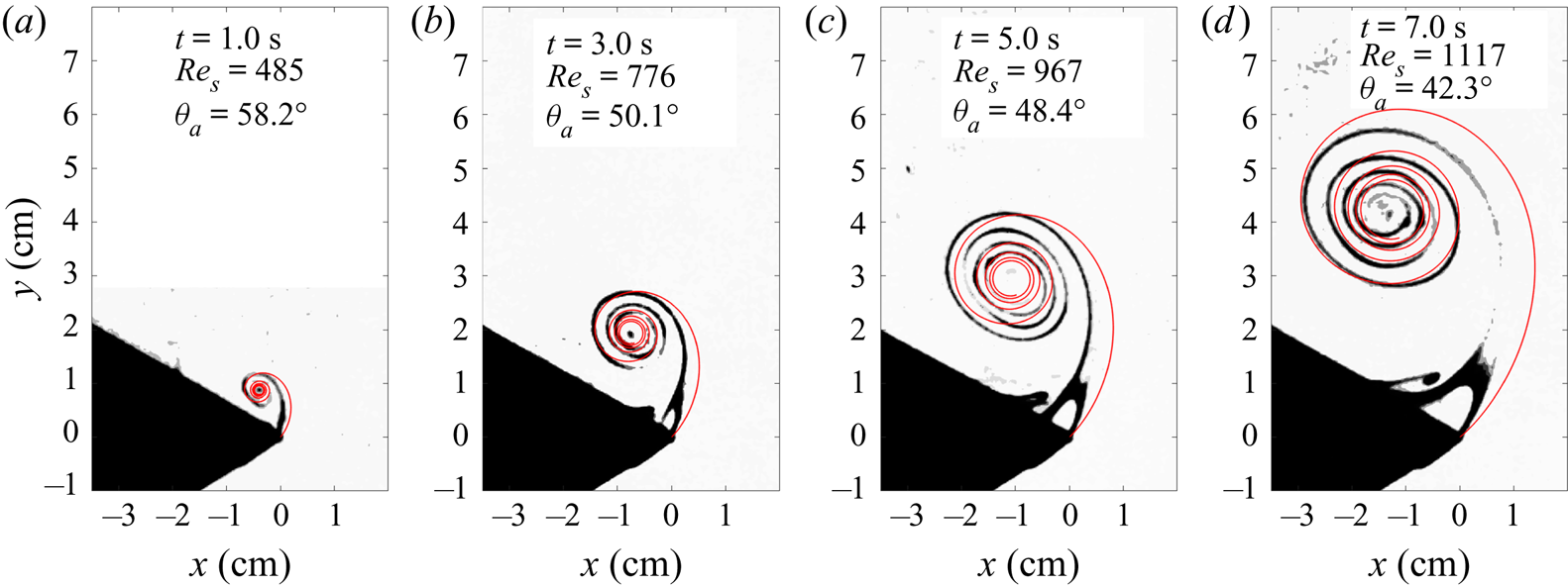
 $Re_s$, which can also be interpreted as a non-dimensional time for the growth of the spiral structure. Figure 5 shows some of their dye visualization images at several different
 $Re_s$ values. Note that the apparent shedding angle is ‘kinked’ well past/above the wedge tangent direction. This feature is shared by the similarity solutions presented in figure 4(b) with shedding angles in figure 3(b). A non-tangential shedding angle requires non-zero entrainment at the apex.
Comparison with the dye visualization experiments of Pullin & Perry (Reference Pullin and Perry1980); images adapted from their figure 5. The similarity sheet shapes (red lines) were matched and converted to the dimensional space by finding the value of  $M$ for which the experimental core position aligned with that of the predicted trajectory. The value of
 $M$ corresponds to a unique value of the shedding angle
 $\theta _a$ as labelled.

Approximate errors between the similarity prediction of Pullin and the experiments of Pullin & Perry (Reference Pullin and Perry1980) for the  $x$- and
 $y$-coordinates of the core position. Much larger errors in the
 $x$-coordinate are due to the experimental measurement itself being a small quantity.

To make comparison to the experiment using a solution from the current study, the measurements of the core position from Pullin & Perry (Reference Pullin and Perry1980) were converted to our similarity space (we note the absorption of the constant  $C$ from (3.3) in their definition of
 $\omega$). The values were then compared to the core trajectory in figure 4(b). It was found that one experimental case intersected the curve and the corresponding solution was transformed to physical space by scaling to the core location. The result is shown in figure 5(d) and exhibits fair agreement considering the somewhat crude assumptions made above about the boundary condition at infinity. However, the experimental shedding angle is still noticeably larger than the predicted one.
Images of the flow development at three earlier times are shown in figure 5(a–c). According to the similarity growth law, for constant parameters the core trajectory in the physical domain follows a constant-angle ray as time increases. This behaviour is clearly not obeyed in the early growth of the spiral. Hence, there must be some other time-dependent effect present in the experiments. We now recall the comments immediately following (3.6) about an implicit time scale that may occur if a time-dependent value is prescribed for any of the input parameters defining the self-similar problem. Figure 5 indicates that this implicit effect manifests as a time-dependent shedding angle  $\theta _a$ at the apex, which is noted as part of the boundary. By (3.8) we can affect a time-dependent shedding angle through different values of the image system scaling
 $M(t)\leftrightarrow \theta _a(t)$. Therefore, we can identify similarity solutions representative of other experimental times by tracing the ray that passes through both the measurement point and the trajectory curve, and again scaling to the core location. The results are overlaid in figure 5(a–c) and also show fair agreement.
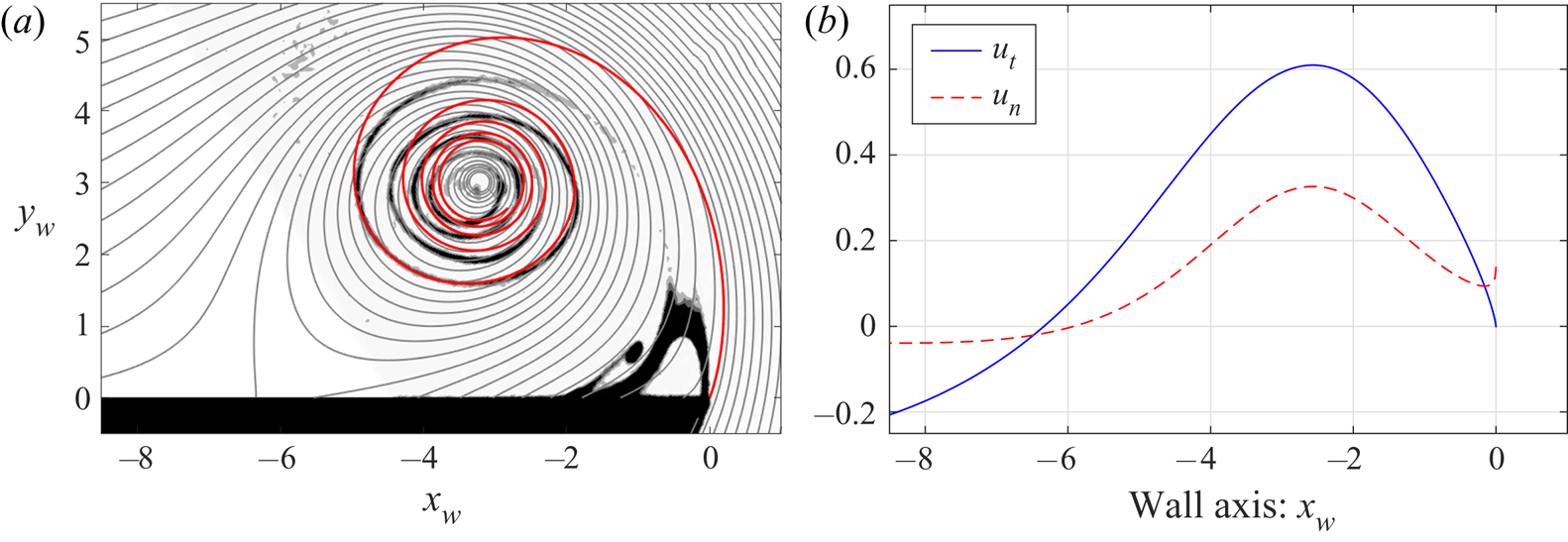
The features of the flow (e.g. shedding angle, core location) are naturally dictated by the boundary conditions. In the experiment, the actual time-dependence and functional connection between these quantities is a more complicated state of affairs. For instance, it is difficult to ascertain the effects, both quantitative and qualitative, of the finite tunnel dimensions or the far-field flow without being given more detailed information. Two physically impactful examples from the experiment are the appearance, near the apex, of a secondary roll-up due to boundary layer separation on the upper wedge face and a corresponding recirculating region, both of opposite sign to the primary separation. Figure 6(a) reproduces the plot of figure 5(d), but with the streamlines of the inviscid flow overlaid. The axes are rotated so that the leeward face is horizontal. The inviscid flow emanates out from the wedge surface, qualitatively capturing the displacement effect of the viscous boundary layer. Figure 6(b) plots the wall-tangential and wall-normal velocity components along the wedge surface. By potential theory, the pressure minimum and velocity maximum must each be located somewhere on the boundary. Moreover, in the similarity space the flow appears steady so that  $(p-p_o)\sim -(u_t^2+u_n^2)$ and these two points coincide. Hence, the separation is correctly placed between the predicted pressure minimum and the apex, occurring almost immediately downstream of the former; see the discussion in Pullin & Perry (Reference Pullin and Perry1980) on page 248 for more. While these results support the ability of the vortex-entrainment sheet model to capture viscous effects, it is noteworthy that the secondary separation bubble is a topological feature that is not possible with the current problem set-up. We believe that proper modelling of this phenomenon ought to involve boundary conditions other than those offered by (2.6) as used presently.
More similarity results for the case in figure 5(d). The  $x_w-y_w$ axes are a right-handed coordinate system on the surface; the scaling was arbitrarily chosen. (a) Overlaid streamlines of inviscid flow (grey lines). (b) Non-dimensional velocities on the upper wall surface:
 $u_t$, tangent component (solid blue);
 $u_n$, normal component (dashed red).

5. Entrainment on the free sheet
Having investigated entrainment solely on the wedge surfaces in § 4, we now present solutions for which the strength ratio distribution on the free sheet is given by a simple function  $\nu (\lambda )$. The image system is defined by
 $c_\gamma =1$,
 $c_q=1$,
 $M=1$, and
 $\varTheta =0$, which corresponds to the standard ‘mirror image’. From (2.8a,b) and (2.7a,b), we have
 $\varGamma _s=-\varGamma _w$ and
 $Q_s=-Q_w$. The problem is then closed upon specification of
 $\tilde {\nu }_o$ and gives the unique outputs
 $J$,
 $\tilde {\nu }_s$, and
 $\omega$. From the results, we will infer some further plausible physical connections between entrainment and viscous effects.
The convergence of the scheme was mostly dependent upon the number of turns resolved in the sheet and thus the (fractional) amount of circulation  $\lambda _c$ contained in those turns. However, global output parameters were remarkably insensitive to
 $\lambda _c$ so long as the first few turns are present. The computational purchase of resolving more turns is the local structure of the sheet shape near the core region. As will be seen below, sheet entrainment eventually brings a given number of turns much closer to the isolated core point. For numerical stability
 $\tilde {\nu }_o$ was treated as the unknown and
 $\tilde {\nu }_s$ was specified instead (see appendix B). Solutions were obtained by incrementing
 $\tilde {\nu }_s$, using the previous solution as an initial condition. The step in
 $\tilde {\nu }_s$ was throttled so that the corresponding change in
 $\lambda _c$ was approximately 1 % of the total circulation.
5.1. Core entrainment
Here, the form of the strength ratio on the sheet is designed so that the entrainment is concentrated toward the spiral core of the sheet, namely
 \begin{equation} \nu(\lambda) = a\lambda^p, \end{equation}
and note that  $a=(1+p)\tilde {\nu }_s$, where the exponent
 $p$ is a parameter that controls the size of the region within which the entrainment is appreciable. Also, since
 $\nu _a=\nu (0)=0$ at the apex, then by (3.8) the shedding angle remains tangential to the lower wedge face.
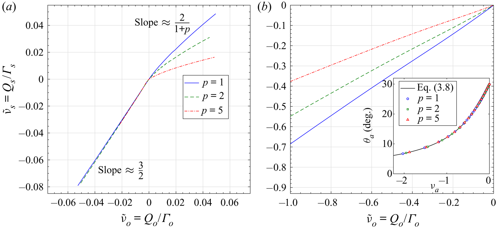
Figure 7(a) plots  $\tilde {\nu }_s$ against
 $\tilde {\nu }_o$ for
 $p=1$, 2, and 5. This plot may essentially be interpreted as a measure of the net sheet entrainment vs. the flux at infinity. For
 $\tilde {\nu }_s<0$ the relationship is almost perfectly linear with slope approximately equal to
 $\tilde {\nu }_s/\tilde {\nu }_o\approx 3/2$, independent of
 $p$. For
 $\tilde {\nu }_s>0$ the slope gradually approaches a constant, but which depends on
 $p$. Below it is shown that as
 $\tilde {\nu }_s>0$ increases, the amount of circulation in the isolated core also increases (or that in the sheet decreases). Moreover, approximately 50 % of this circulation resides within a very small radius around the core. By approximating this portion of the sheet with the single core point, the relationship
 $\tilde {\nu }_s/\tilde {\nu }_o\sim (1+p)^{-1}$ can be inferred from the Kutta conditions in (3.6).
The average strength ratio on the sheet  $\tilde {\nu }_s=Q_s/\varGamma _s$ vs. the boundary condition at infinity
 $\tilde {\nu }_o=Q_o/\varGamma _o$. (a) Core entrainment with the
 $\nu (\lambda )$ distribution given by (5.1). (b) Apex entrainment with the
 $\nu (\lambda )$ distribution given by (5.2). The inset plots the shedding angle
 $\theta _a$ vs. the strength ratio at the apex
 $\nu _a=\nu (0)$; the line is the asymptotic theory while symbols are directly measured from the numerical solutions.

Next, we recall that  $\tilde {\nu }_s<0$ corresponds to flow exiting the sheet, while
 $\tilde {\nu }_s>0$ represents flow entering the sheet. Hence, for this problem set-up, there is a respective efflux and influx of fluid across the boundary
 $C_\infty$ at infinity since
 $\tilde {\nu }_o$ shares the same sign. A similar phenomenon occurs for Falkner–Skan boundary layers, whereby the vertical flow at infinity changes from an efflux to an influx as the outer flow acceleration is increased, which competes with the displacement of the layer growth due to diffusion (see DeVoria & Mohseni Reference DeVoria and Mohseni2019). Motivated by this, we label
 $\tilde {\nu }_s<0$ as ‘diffusion-dominated entrainment’ (DDE) and
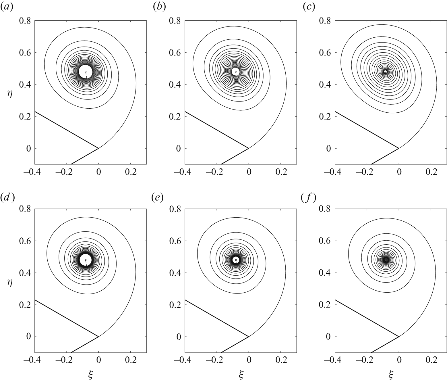
 $\tilde {\nu }_s>0$ as ‘inertia-dominated entrainment’ (IDE). To give credence to these assignations, figure 8(a–f) plots several examples for each entrainment type with
 $p=1$ as the exponent in (5.1); the baseline case of
 $\tilde {\nu }_s=0$ is shown in figure 8(d). For DDE the outer turns of the spiral gradually spread outward, while the inner most turns concentrate much closer toward the isolated core point. Moreover, as indicated in each panel, the circulation contained in the resolved sheet
 $\lambda _c$ rapidly increases, reaching 99.9 % at
 $\tilde {\nu }_s=-0.035$; all cases maintained 20 turns. As such, the effect of the core point is negligible as its circulation has been almost entirely redistributed or spread out along the sheet. The total circulation
 $J$ increased/decreased with
 $\tilde {\nu }_s$ by less than 1 % over the range shown in the figure. The IDE cases have an opposing trend with circulation being transported from the sheet to the core point with fractional circulation (
 $1-\lambda _c$). Consequently, the spiral is drawn closer to the core point owing to its sink-like entrainment. However, the turns maintain their tightly wound spacing and also become more circular with any ellipticity practically vanishing. In general, while there is a significant change in the spacing of the turns, the large-scale dimensions and position of the core point are essentially unaffected for all cases.
Self-similar sheet shapes with entrainment concentrated near the core region. The strength ratio is given by (5.1) with  $p=1$. (a–c) Diffusion-dominated entrainment:
 $\tilde {\nu }_s<0$. (d–f) Inertia-dominated entrainment:
 $\tilde {\nu }_s\geq 0$; (d) is the baseline case. Each case has 20 resolved turns and
 $\lambda _c$ is the fraction of the total circulation contained in these turns. (a)
 $\tilde {\nu }_s=-0.013, \lambda _c=0.952$, (b)
 $\tilde {\nu }_s=-0.022, \lambda _c=0.991$, (c)
 $\tilde {\nu }_s=-0.035, \lambda _c=0.999$, (d)
 $\tilde {\nu }_s=0, \lambda _c=0.752$, (e)
 $\tilde {\nu }_s=0.005, \lambda _c=0.650$ and (f)
 $\tilde {\nu }_s=0.010, \lambda _c=0.562$.

The features in figure 8 may be readily interpreted through a relevant aerodynamic application, namely the spanwise flow often observed in leading-edge vortices. This phenomenon has been thought to be a stabilizing mechanism in rotating wing lift generation (e.g. Ellington et al. Reference Ellington, van den Berg, Willmott and Thomas1996). Here, this flow would be out-of-plane and IDE would correspond to removal of in-plane fluid (stabilizing), while DDE injects fluid into the plane due to a decelerating spanwise flow causing growth of the vortex.
5.2. Apex entrainment
In this section we give a similar analysis for a strength ratio that concentrates the entrainment near the apex, namely
 \begin{equation} \nu(\lambda) = a(1-\lambda)^p. \end{equation}
Again we have  $a=(1+p)\tilde {\nu }_s$ and this is also equal to the strength ratio at the apex
 $\nu _a$. Figure 7(b) plots the corresponding
 $\tilde {\nu }_s$ vs.
 $\tilde {\nu }_o$ for different values of
 $p$. Some solutions for small positive values of
 $\tilde {\nu }_o$ were obtained, but the iterative solver soon became extremely slow to converge. Moreover, it was evident that the sheet shape at the apex did not agree with the shedding angle given by (3.8). We concluded, then, that the boundary conditions for this particular self-similar problem do not admit solutions for
 $\tilde {\nu }_o>0$ when the entrainment is non-zero at the apex.
For  $\tilde {\nu }_o<0$ we again see a linear relationship to
 $\tilde {\nu }_s$ and with a slope that depends on
 $p$. Since the entrainment is concentrated at the apex, the inner structure of the spiral remains relatively unchanged, whereas the orientation of the spiral and the core point location are drastically altered. For instance, the variable shedding angle is plotted vs. the strength ratio at the apex as the inset of figure 7(b). Both direct measurements of
 $\theta _a$ from the sheet shape and (3.8) are shown, thus further validating the asymptotic theory. Again adopting the label DDE for
 $\tilde {\nu }_s<0$, we see that the ‘diffusion’ near the apex results in
 $\theta _a$ approaching the wedge bisector. The larger magnitudes of
 $\tilde {\nu }_o=-U_n/U_t$ compared to § 5.1 occur because, below a certain value, the core structure essentially convects downstream while remaining connected to the apex by a long ‘umbilical’. Although the physical flow at infinity is not uniform, we may draw a qualitative analogy with the angle of attack of an airfoil. For our chosen orientation of the wedge geometry, the
 $U_t$ component represents a vertical plunge, while
 $U_n$ represents a streamwise component. Therefore, we can rotate our reference to define an angle of attack as
 $\alpha ={\rm \pi} /2+\arctan (\tilde {\nu }_o)$ so that the motion corresponds to a leftward surge of the ‘airfoil’ at angle of attack
 $\alpha$ relative to the horizontal.
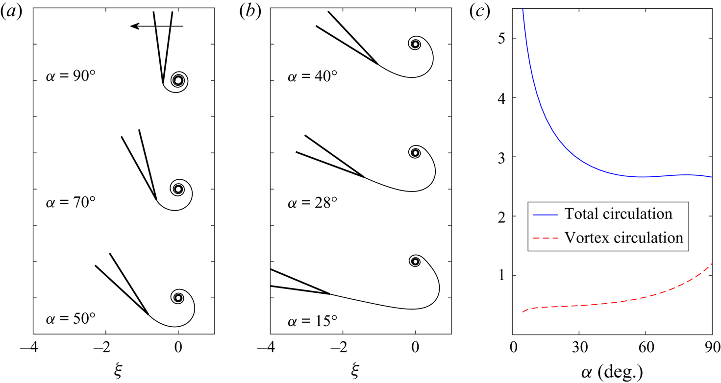
To illustrate this concept, we computed solutions for a  $\beta _a=15^{\circ }$ wedge representing a thin, but finite-angled trailing edge. The exponent value
 $p=5$ was chosen so that the sheet entrainment was restricted to the apex region. Figure 9(a,b) plot a series of such solutions, where again the angle of attack
 $\alpha$ is measured from the horizontal to the wedge bisector or chord line. As
 $\alpha$ decreases, the size of the rolled-up core appears to decrease. Figure 9(c) plots the total circulation in the sheet
 $J$ along with the circulation contained in the isolated core vortex
 $J(1-\lambda _c)$. The latter quantity depends on the number of resolved turns, however, this was the same for each case (five turns). The vortex circulation decreases with
 $\alpha$, indicating a weaker starting vortex at lower angles of attack. Conversely, the total circulation increases as
 $\alpha$ decreases, but this corresponds to the longer arclength of the shed sheet. For
 $\alpha \rightarrow 0$, these results indicate that the umbilical sheet is infinitely long and the starting vortex core is at infinity, which agrees with Prandtl's classical aerodynamics description of steady lift. However, the vorticity of infinite total circulation (
 $J\rightarrow \infty$) is distributed along the sheet with a vanishingly weak starting vortex, which is similar to Wagner's lift development.
(a,b) Examples of the airfoil analogy with trailing-edge separation. The motion is a leftward surge at angle of attack  $\alpha ={\rm \pi} /2+\arctan (\tilde {\nu }_o)$ measured from the horizontal to the wedge bisector (i.e. chord line). The wedge angle is
 $\beta _a=15^{\circ }$. (c) The total circulation in the sheet (solid blue) and the isolated vortex circulation (dashed red) as functions of
 $\alpha$.

6. Conclusion
Building off previous work by the authors, this paper explored the potential to capture viscous flow effects using an inviscid model with singular sheets of discontinuity taking the place of the actual viscous layers. The case study used was starting flow separation over a sharp wedge. Specifically, the self-similar solutions originally computed by Pullin (Reference Pullin1978) were significantly augmented by including entrainment. This was accomplished by consideration of a broader class of boundary conditions for the problem. The specification of these conditions is tantamount to supplying the entrainment. This is a consequence associated with foregoing a fluid description whose governing equation is able to accommodate more independent boundary conditions.
Mass flux into the boundaries, represented as vortex-entrainment sheets, is allowed by relaxing the usual, yet axiomatically assumed normal boundary condition of no through flow. This mass entrainment offers a more thorough dynamical inviscid model which, in particular, is argued to represent viscous effects. For example, global quantities, such as the total circulation, as well as local quantities, such as the shedding angle, sheet strength and velocity at the apex, may all be manipulated through the entrainment. Several computed solutions were presented and showed favourable agreement with an existing experimental work. Moreover, some phenomena in the experiment attributed to viscous effects were captured, qualitatively at the very least, by the inviscid model. When the entrainment was specified on the freely shed sheet, some familiar features commonly encountered in aerodynamic applications were observed. It was argued that the displacement effect/velocity of a thickening layer is represented by ‘diffusion-dominated entrainment’, for which mass/fluid emanates out of the sheet. In a similar manner, a sink-like flow into the sheet corresponds to ‘inertia-dominated entrainment’, for which large accelerations or fast velocities generate strong vorticity. Consequently, the vorticity becomes increasingly concentrated within a tightly wound spiral core.
As a whole, we interpret the model features to be the representation of a finite Reynolds number. Of course, the fidelity of the inviscid results depends on the level of information contained in the entrainment boundary condition. Ideally, the local entrainment function would correspond to that of the actual boundary layers. However, we likely will not be given this detailed distribution a priori, but instead will have certain global quantities that must be satisfied on physical grounds for a certain problem, such as a net force, the rate of mass consumption or energy dissipation. In turn, these quantities could be used to determine some of the free parameters in the present model, such as the averaged strength ratio for a given sheet. This is an ideal task for future work. Other relevant studies may focus on practical applications, such as flow control devices for manipulation of fluid–structure interactions. Here, entrainment from solid surfaces can be directly imposed through mechanisms injecting/suctioning mass into/from the fluid.
Acknowledgements
We wish to acknowledge the partial support of the NSF and ONR in this work.
Declaration of interests
The authors report no conflict of interest.
Appendix A. Asymptotic solution near the apex
In this appendix the asymptotic solution for  $\omega (\lambda )\rightarrow 0$ (with
 $\lambda \rightarrow 0$) is given. This analytically determines the shedding angle of the free sheet as well as the strengths of the vortex and entrainment sheets at the apex:
 $\gamma _a$ and
 $q_a$. The results are not specific to the assumed forms of
 $\nu (\lambda )$ used above and thus are applicable to arbitrary strength ratios. Moreover, while we use the non-dimensional self-similar equations in § 3 to proceed here, the same basic analysis is valid on the general equations of § 2.
Using the vector Kutta condition in (3.6), we can rewrite (3.5) as
 \begin{equation} (1-n)\left[\bar{\omega}+Q_P(1-\lambda)\frac{\textrm{d}\bar{\omega}}{\textrm{d}\lambda}\right]=nJ\omega^{2n-1}G(\omega), \end{equation}
where the function  $G(\omega )$ is defined similar to that in Pullin as
 \begin{equation} G(\omega)=\frac{1}{2{\rm \pi} i}\int_0^1\left[\frac{1-i\nu(\lambda^\prime)}{\omega^{\prime n}(\omega^n -\omega^{\prime n})}+\frac{c_\gamma-ic_q\nu(\lambda^\prime)}{\overline{A^n\omega^{\prime n}}(\omega^n +\overline{A^n\omega^{\prime n}})}\right]\,\textrm{d}\lambda^\prime. \end{equation}
Next, take  $\omega =K\lambda ^\mu$ where
 $K=|K|\,\textrm {e}^{\textrm {i}\theta _a}$ and
 $\theta _a$ is the argument of an infinitesimal length of the sheet at the apex measured anticlockwise positive from the wedge bisector and thus is the shedding angle. With this form of
 $\omega (\lambda )$ the behaviour of the
 $G(\omega )$ integral as
 $\omega \rightarrow 0$ can be obtained from Muskhelishvili (Reference Muskhelishvili1946). Upon substitution into (A 1) it can be shown that
 $\mu =1$ to match leading orders of
 $\lambda$, and subsequently that
 \begin{equation} |K|^2=\frac{J}{2(1-n)Q_P}\left\{\frac{\bar{A}(1-i\nu_a)\cos\beta{\rm \pi} -(c_\gamma -ic_q\nu_a)\,\textrm{e}^{\textrm{i}2\theta_a}}{-i\bar{A}\sin\beta{\rm \pi} }\right\}, \end{equation}
where  $\nu _a=\nu (0)$ is the value of the strength ratio at the apex. The term in curly brackets, say
 $P$, must then be purely real, which determines the shedding angle as
 \begin{equation} \theta_a=\pm\frac{1}{2}\left[\arccos\left(\frac{M\cos\beta{\rm \pi} }{c_\gamma\sqrt{1+c_a^2}}\right) +\arctan(c_a)-\varTheta\right], \end{equation}
where  $(\pm )=\text {sgn}(U_t)$,
 $c_a=c_q\nu _a/c_\gamma$ and recall that
 $A=M\,\textrm {e}^{\textrm {i}\varTheta }$. Then
 $P\in \mathbb {R}$ is given by
 \begin{equation} P=\frac{\nu_a\cos\beta{\rm \pi} +c_\gamma\sqrt{(1+c_a^2)/M^2-(\cos^2\beta{\rm \pi} )/c_\gamma^2}}{\sin\beta{\rm \pi} }. \end{equation}
That  $P$ remains real and strictly positive gives obvious restrictions on the parameters involved. In particular,
 $0<M< M_{max}$ where
 $M_{max}^2=(c_\gamma ^2+c_q^2\nu _a^2)/\cos ^2\beta {\rm \pi}$. Next, we have
 \begin{equation} G(\omega)=\frac{\omega^{1-2n}P}{2nK}+G^*(\omega),\quad |K|=\left[\frac{JP}{2(1-n)Q_P}\right]^{{1}/{2}}, \end{equation}
where  $\omega ^{2n-1}G^*(\omega )\rightarrow 0$ as
 $\omega \rightarrow 0$. The Plemelj formulae give the complex velocities on the leeward (
 $+$) and windward (
 $-$) sides of the sheet at the apex for
 $U_t>0$ as
 \begin{equation} \left.\frac{\textrm{d}\varOmega}{\textrm{d}\omega}^{\pm}\right|_{\omega=0}=(u_{t,a}^{\pm}-iu_{n,a}^{\pm})= \frac{JP}{2|K|}\left[1\mp\frac{1-i\nu_a}{P}\right], \end{equation}
where  $u_{t,a}$ and
 $u_{n,a}$ are, respectively, the tangential and normal components relative to the sheet. By definition, the strengths of the vortex and entrainment sheets are
 \begin{equation} \gamma_a = u_{t,a}^{-}-u_{t,a}^{+} = \frac{J}{|K|},\quad q_a = u_{n,a}^{-}-u_{n,a}^{+} = \nu_a\frac{J}{|K|}, \end{equation}
and thus  $q_a/\gamma _a=\nu _a$ as required. Likewise, the sheet velocities (i.e. principal value) are
 \begin{equation} u_{t,a}=\frac{1}{2}(u_{t,a}^{+}+u_{t,a}^{-})=\frac{JP}{2|K|},\quad u_{n,a}=\tfrac{1}{2}(u_{n,a}^{+}+u_{n,a}^{-})=0. \end{equation}
For  $U_t<0$ the (
 $\mp$) in (A 7) is simply inverted to
 $(\pm )$, which changes the signs of
 $\theta _a$ and
 $\gamma _a=u_{t,a}^{-}-u_{t,a}^{+}$ from positive to negative, while the entrainment
 $q_a=u_{n,a}^{-}-u_{n,a}^{+}$ takes a sign in accordance with
 $q_a=\nu _a\gamma _a$.
Appendix B. Numerical scheme
Here, we detail the method used by Pullin along with the modifications required to include entrainment. The reader is referred to his paper for additional information.
The sheet is represented by  $k=1,\ldots ,N$ planar segments with circulation
 $\lambda _{k-1}<\lambda \leq \lambda _k$ and with endpoints
 $\omega _{k-1}$ and
 $\omega _k$. The isolated point singularity is located at
 $\omega _{N+1}=\omega _c=r_c\,\textrm {e}^{\textrm {i}\theta _c}$ with net strength
 $J(1-\lambda _N)(1-i\tilde {\nu }_c)$ where
 $\lambda _N=\lambda _c$ and
 $\omega _N=\omega _s$. Finite difference versions of (3.5) are solved at the midpoints defined as
 \begin{equation} \omega_{k-1,k}=\tfrac{1}{2}(\omega_{k-1}+\omega_k),\quad \lambda_{k-1,k}=\tfrac{1}{2}(\lambda_{k-1}+\lambda_k)\quad \{k=1,\ldots, N\}. \end{equation}
The derivative  $\textrm {d}\bar {\omega }/\textrm {d}\lambda$ is computed with a central difference and all integration is performed with the trapezoidal rule. As such, the system (3.5)–(3.7) can be written as
 \begin{equation} \left.\begin{array}{c@{}} \begin{aligned} 0 & = (1-n)\left[\bar{\omega}_{k-1,k}+Q_P(1-\lambda_{k-1,k}) \left(\dfrac{\bar{\omega}_k-\bar{\omega}_{k-1}}{\lambda_k-\lambda_{k-1}}\right)\right]\nonumber\cr & \quad +in(\omega_{k-1,k})^{n-1}\left\{(1-i\tilde{\nu}_o)+\dfrac{J}{2{\rm \pi} } \sum_{j=0}^{N+1} F_j(\omega_{k-1,k})A_j\right\}, \end{aligned}\\ \displaystyle 0= \left\{(1-i\tilde{\nu}_o)-\dfrac{J}{2{\rm \pi} }\sum_{j=0}^{N+1} \left(H^\gamma_jB_j-iH^q_jC_j\right)\right\}, \nonumber\\ \displaystyle 0= (1-n)\left[\bar{\omega}_{N+1}+Q_P\left(\dfrac{\bar{\omega}_{N+1} -\bar{\omega}_N}{1-i\nu_{N+1}}\right)\right] +in(\omega_{N+1})^{n-1}\left\{(1-i\tilde{\nu}_o)+\dfrac{J}{2{\rm \pi} }\sum_{j=0}^{N+1} G_jA_j\right\}, \end{array}\right\} \end{equation}
with  $Q_P=(n+2m)/(1+m)$ and
 \begin{equation} \left.\begin{array}{c@{}} \displaystyle F_j(\omega_{k-1,k})=\left[\dfrac{1-i\nu_j}{\omega_{k-1,k}^n-\omega_j^n}+ \dfrac{-(c_\gamma-ic_q\nu_j)}{\omega_{k-1,k}^n+\overline{A^n\omega_j^n}}\right],\\ \displaystyle \nu_j=\nu(\lambda_j),\quad \nu_{N+1}=\tilde{\nu}_c=\dfrac{1}{1-\lambda_N} \int_{\lambda_N}^1\nu(\lambda)\,\textrm{d}\lambda,\\ \displaystyle G_j=F_j(\omega_{N+1}), \quad G_{N+1}=\left[\dfrac{-(c_\gamma-ic_q\nu_{N+1})}{\omega^n_{N+1}+ \overline{A^n\omega^n_{N+1}}}+\dfrac{(n-1)(1-i\nu_{N+1})}{2n\omega^n_{N+1}}\right], \\ \displaystyle H^\gamma_0=H^\gamma_1,\quad H^q_0=H^q_1,\quad H^\gamma_j= \dfrac{\overline{A^n\omega_j^n}+c_\gamma\omega_j^n}{\overline{A^n}|\omega_j^n|^2}, \quad H^q_j=\dfrac{\overline{A^n\omega_j^n}+c_q\omega_j^n}{\overline{A^n}|\omega_j^n|^2}, \end{array}\right\} \end{equation}
where the two terms in  $G_{N+1}$ are the velocities due to the image of the isolated point singularity and the Routh correction (
 $f^{\prime \prime }/2(\,f^\prime )^2$ where
 $f(z)=z^{n}$), respectively, and
 \begin{equation}
\left.\begin{array}{c@{}} \displaystyle
A_0=\tfrac{1}{2}(\lambda_1-\lambda_0),\quad
A_N=\tfrac{1}{2}(\lambda_N-\lambda_{N-1}),\quad
A_{N+1}=1-\lambda_N,\\ \displaystyle
A_j=\tfrac{1}{2}(\lambda_{j+1}-\lambda_{j-1})\quad
\{\,j=1,\ldots, N-1\},\\ \displaystyle
B_0=\dfrac{\lambda_1}{1-n},\quad
B_1=\tfrac{1}{2}(\lambda_2-\lambda_1),\quad B_j=A_j \quad
\{\,j=2,\ldots, N+1\},\\ \displaystyle
C_0 =
\lambda_1^n\int_0^{\lambda_1}\dfrac{\nu(\lambda)}{\lambda^n}\,\textrm{d}\lambda,\quad
C_j = B_j\nu_j \quad \{\,j=1,\ldots, N+1\}.
\end{array}\right\} \end{equation}
The  $C_0$ term and the average
 $\nu _{N+1}=\tilde {\nu }_c$ each depend on the strength ratio distribution
 $\nu (\lambda )$. For the two cases of (5.1) and (5.2) studied in this paper
 \begin{gather} \text{Eqn. ({5.1}):}\quad \widetilde{\nu_c}= a\left[\frac{1-\lambda_N^{1+p}}{(1+p)(1-\lambda_N)}\right], \quad C_0=a\left[\frac{\lambda_1^{1+p}}{1+p-n}\right], \end{gather}
 \begin{gather}\text{Eqn. ({5.2}):}\quad \widetilde{\nu_c}= a\left[\sum_{k=0}^p \binom{p}{k}\frac{(-1)^k(1-\lambda_N^{1+k})}{(1+k)(1- \lambda_N)}\right], \quad C_0=a\left[\sum_{k=0}^p \binom{p}{k}\frac{(-1)^k\lambda_1^{1+k}}{1+k-n}\right]. \end{gather}
For each case,  $a=(1+p)\tilde {\nu }_s$. The actual scheme used makes the following transformation:
 \begin{equation} \omega_j=\omega_{N+1}-\rho_j\,\textrm{e}^{\textrm{i}(\vartheta_j+\theta_c)}, \end{equation}
and recalling that  $\omega _{N+1}=r_c\,\textrm {e}^{\textrm {i}\theta _c}$, the
 $\vartheta _j$ are then measured anticlockwise positive from the line connecting
 $\omega _{N+1}$ and the origin, and the
 $\rho _j$ are the corresponding radii measured from
 $\omega _{N+1}$ to each
 $\omega _j$. The angles
 $\vartheta _j$ are held constant and the values of
 $\lambda _j$ are unknowns to be determined. Treating
 $\tilde {\nu }_s$ as unknown results in poor convergence as it quantifies the normal boundary condition on the sheet. Therefore, we instead take
 $\tilde {\nu }_o$ as unknown and specify
 $\tilde {\nu }_s$. By locating the wedge apex at
 $\omega _0=0+i0$ and since
 $\lambda _0=0$, we then have a
 $2N+4$ system of equations expressed by
 \begin{equation} {\boldsymbol{f}}({\boldsymbol{x}})=\textbf{0}, \quad {\boldsymbol{x}}=(\rho_1,\rho_2,\ldots,\rho_N, \lambda_1,\lambda_2,\ldots,\lambda_N,r_c,\theta_c,J,\tilde{\nu}_o). \end{equation}
For the cases with  $\tilde {\nu }_o=0$ and variable
 $M$ in § 4.2, the former was replaced with
 $\varTheta$ as the unknown to be obtained. The system is iteratively solved with the fsolve function in Matlab until the Euclidean vector norm of
 ${\boldsymbol{f}}({\boldsymbol{x}})$ is less than
 $\epsilon =10^{-10}$.