1 Introduction
Hydraulic fracturing is widely used to measure in situ stresses (Zoback et al. Reference Zoback, Rummel, Jung and Raleigh1977) and to create permeable pathways in the deep subsurface to enhance heat production from geothermal reservoirs (Legarth, Huenges & Zimmermann Reference Legarth, Huenges and Zimmermann2005), accelerate waste remediation (Frank & Barkley Reference Frank and Barkley1995) and to stimulate production from oil and gas wells (Economides & Nolte Reference Economides and Nolte2000). In this technique, high-pressure fluid is injected into an isolated portion of a well to initiate and propagate a fracture through the formation. At some point, proppant is pumped in as a slurry with the injection fluid, is transported along the advancing fracture and remains in the fracture at shut-in to prop open the fracture. This retains the fluid conductivity of the introduced fracture.
Modelling hydraulic fracturing is challenging since a variety of physical processes are involved. These include fracture propagation and inflation, fluid flow within the fracture, proppant transport and settling, followed by fracture deflation, closure and proppant capture. These processes may be represented by making appropriate simplifying assumptions in the analysis. For the fracture propagation and fluid flow within it, it is typical to include simplification of the fracture geometry as a planar form, treating the inflating fluid as Newtonian, and assuming flow to be laminar. Various models follow this formalism to approximately define the development of fracture geometry, among which the PKN and KGD models are the most popular (Khristianovic & Zheltov Reference Khristianovic and Zheltov1955; Perkins & Kern Reference Perkins and Kern1961; Greetesma & de Klerk Reference Greetesma and de Klerk1969; Nordgren Reference Nordgren1972). More representative models have relaxed these assumptions, such as models that accommodate non-Newtonian fluids and poroelastic effects (Detournay, Cheng & McLennan Reference Detournay, Cheng and McLennan1990), turbulent fluid flow (Zolfaghari, Dontsov & Bunger Reference Zolfaghari, Dontsov and Bunger2018), and non-local elasticity for the blade-like fracture (Adachi & Peirce Reference Adachi and Peirce2008). Comprehensive reviews of these models can be found in Adachi et al. (Reference Adachi, Siebrits, Peirce and Desroches2007), Rahman & Rahman (Reference Rahman and Rahman2010), Detournay (Reference Detournay2016) and Lecampion, Bunger & Zhang (Reference Lecampion, Bunger and Zhang2018), among others. In addition, approaches have been advanced to model fracturing process and associated fluid flow using continuum and discrete approaches (Jing Reference Jing2003; Zhang, Dontsov & Mack Reference Zhang, Dontsov and Mack2017; Wang et al. Reference Wang, Elsworth, Wu, Liu, Zhu and Liu2018b ; Zhang et al. Reference Zhang, Ma, Wu and Meng2018).
Proppant transport and placement poses an additional challenge to the modelling of hydraulic fracturing. The fluid–solid two-phase system is often modelled under the Eulerian–Eulerian framework (Ouyang, Carey & Yew Reference Ouyang, Carey and Yew1997; Shiozawa & McClure Reference Shiozawa and McClure2016), while sometimes the Eulerian–Lagrangian approach is used to allow models to track individual proppant particles (Dontsov & Peirce Reference Dontsov and Peirce2015a ; Zhang, Li & Gutierrez Reference Zhang, Li and Gutierrez2017). The slurry is usually represented as a fluid–solid mixture of prescribed rheology and density with differential settling enabled from the suspension. In addition, common assumptions are that the proppant is distributed uniformly across the fracture aperture and that slip between proppant and the carrier fluid is only due to the gravitational settling (Adachi et al. Reference Adachi, Siebrits, Peirce and Desroches2007). However, proppant tends to migrate transversely away from the fracture walls to accumulate at the fracture centre, where shear stress is the lowest and flow velocity is the highest. This effect may also be accommodated (Dontsov & Peirce Reference Dontsov and Peirce2014), where the governing equations for slurry flow and proppant transport may be derived using an empirical law for slurry (Boyer, Guazzelli & Pouliquen Reference Boyer, Guazzelli and Pouliquen2011).
The fracture geometry and distribution of the encased proppant condition the closure behaviour of the fracture as the hydraulic pressure is released, and this ultimately determines fracture conductivity – a key parameter controlling well performance. The residual aperture profile of a hydraulic fracture filled with a basal proppant bank may be determined by assuming a power-law increase in stress at the top of the bank, and in prescribing a certain degree of compaction of the proppant bank (Warpinski Reference Warpinski2010). Results show that an open-arch zone is formed above the proppant bank where high-conductivity pathways endure and play a significant role in well performance (Cipolla et al. Reference Cipolla, Lolon, Mayerhofer and Warpinski2009; Liu et al. Reference Liu, Leung, Chalaturnyk, Virues and Ulc2017). Based on the Distributed Dislocation Technique, Neto & Kotousov (Reference Neto and Kotousov2013a ,Reference Neto and Kotousov b ), Khanna, Neto & Kotousov (Reference Khanna, Neto and Kotousov2014) and Neto, Khanna & Kotousov (Reference Neto, Khanna and Kotousov2015) developed models to define residual opening and conductivity of a KGD fracture partially filled with a symmetric (about the axis of the fracture) proppant pack. These studies confirm the crucial impact of proppant distribution and its mechanical properties on well performance. The current study utilizes a fracture-propagation, proppant-transport and fracture-deflation approach (Wang & Elsworth Reference Wang and Elsworth2018) with an arbitrary distribution of proppant, and thus is capable of evaluating the conductivity of the closed fracture, with few restrictions, once the fracture geometry and final proppant distribution are obtained.
We develop, then use a numerical model to follow the evolution of fracture footprint, fracture aperture distribution, and proppant distribution, to define conductivity evolution of the hydraulic fracture, which is partially filled by proppant, during shut-in, flowback and then production. The details of this model are provided, including assumptions, governing equations and the numerical algorithm. Parametric studies are then completed to investigate the effects of fluid viscosity, proppant size, proppant density and leak-off rate on fracture propagation, proppant distribution and conductivity distribution following fracture closure. Finally, reservoir simulations are conducted to visualize the distribution of fluid transport inside the hydraulic fractures during production.
2 Mathematical formulation
2.1 Background and assumptions
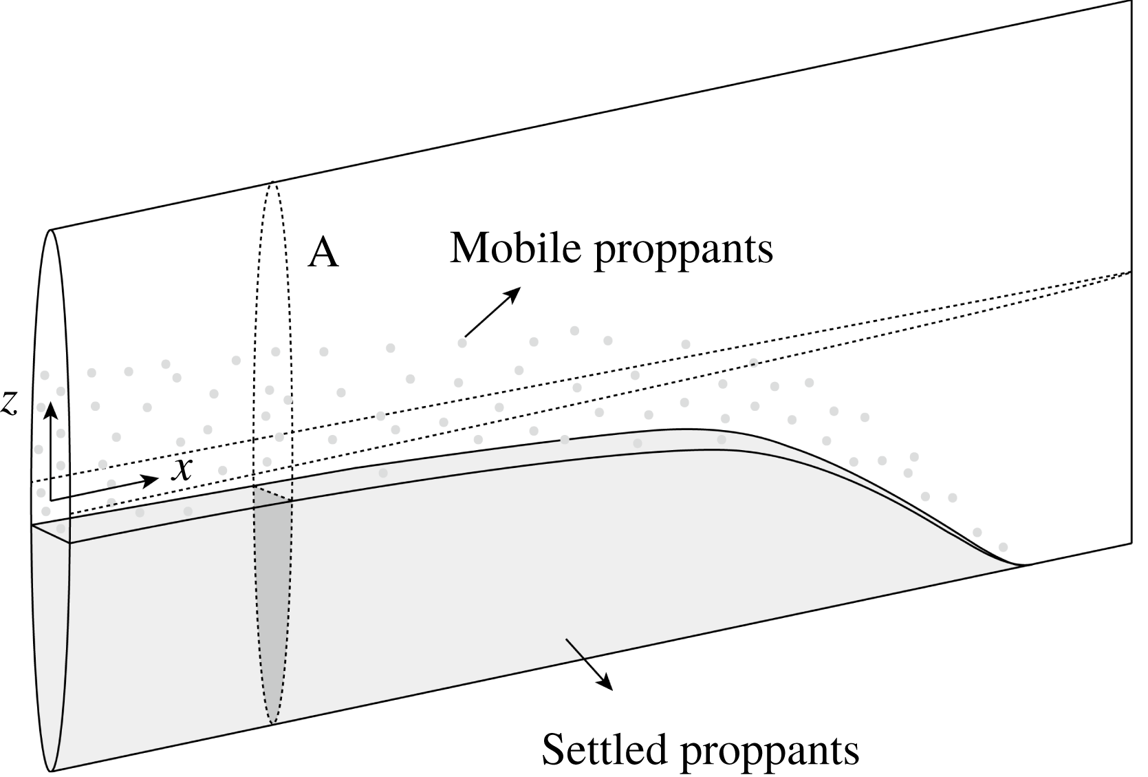
The fracture-propagation model is developed in two dimensions based on the classical PKN-formalism (Perkins & Kern Reference Perkins and Kern1961; Nordgren Reference Nordgren1972). This assumes that the propagating fracture is vertical, has a constant height and is of elliptical cross-section. A schematic of the fracture and the associated coordinate system is shown in figure 1, where
 $x$
is the ordinate along the fracture in the horizontal direction and
 $z$
is the vertical ordinate. Fluid pressure in the fracture is assumed to be uniform over the height of the fracture. An approximation is made that plane strain prevails in planes perpendicular to the direction of propagation. These general assumptions of the PKN model are encumbered by two principal limitations: (i) the plane strain approximation is true only sufficiently distant from the fracture tip and when the fracture width and pressure vary smoothly along the fracture length direction, and (ii) the application of the model is constrained to situations where the toughness of the rock is negligible – both situations that are close to reality for large blade-like fractures. In addition, the PKN model is sufficiently capable of providing a test bed for modelling proppant transport and fracture deflation – its utility here. These two principal limitations of the model can be overcome by introducing a non-local elasticity equation (Adachi & Peirce Reference Adachi and Peirce2008; Dontsov & Peirce Reference Dontsov and Peirce2015b
, Reference Dontsov and Peirce2016).
Schematic of proppant transport in a propagating blade-shaped fracture.

The proppant transport is modelled by representing the fluid–solid mixture, i.e. the slurry, as a two-component, interpenetrating continuum. The distribution of proppant in the fracture is defined in terms of its volumetric concentration
 $\unicode[STIX]{x1D719}$
, and is normalized as
 $$\begin{eqnarray}\bar{\unicode[STIX]{x1D719}}=\frac{\unicode[STIX]{x1D719}}{\unicode[STIX]{x1D719}_{max}},\end{eqnarray}$$
where
 $\unicode[STIX]{x1D719}_{max}$
is the maximum allowable volumetric concentration determined from geometrical considerations. It is assumed that all proppant particles are spheres of the same radius, and both proppant and fluid are incompressible. An empirical constitutive law for the slurry (Dontsov & Peirce Reference Dontsov and Peirce2014) is used to describe the rheology of the slurry, the transition from Poiseuille flow to Darcy filtration flow, proppant motion with fluid flow and proppant gravitational settling.
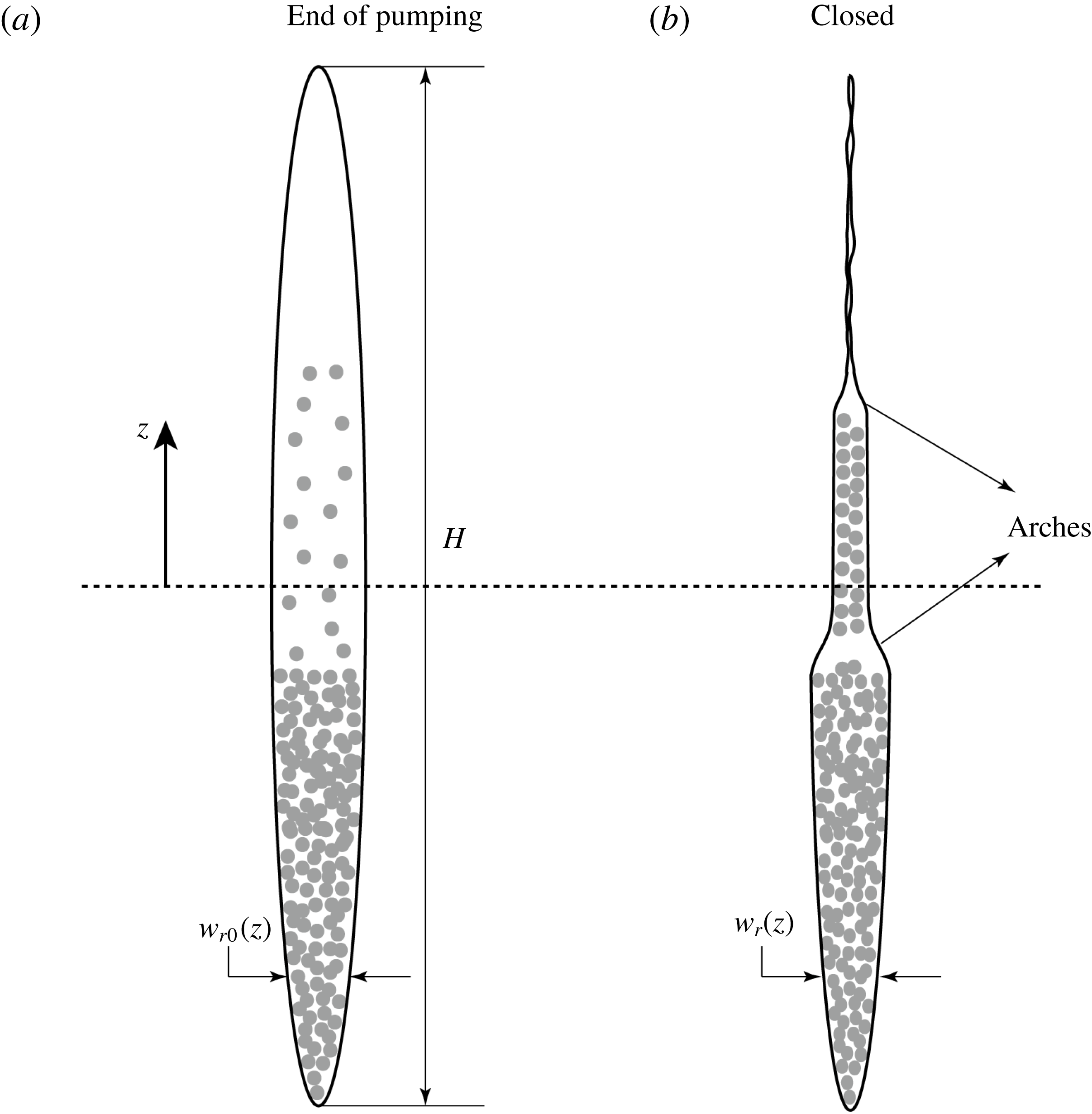
The fracture closure model assumes that leak-off of the residual fracturing fluid into the surrounding formation is sufficiently rapid that the fracture stops propagating and proppant stops moving once pumping stops. During shut-in, flowback and production stages, decreasing hydraulic pressure allows the fracture to deflate and to compact the encased proppant pack. Compaction of the pack is also accompanied by flexural displacement of the unsupported spans of the fracture – leaving residual apertures absent proppant (in the arched channel), as shown by the schematics in figure 2. This can lead to a complex distribution and evolution of the fracture conductivity, which has a significant influence on well performance and on the evolution of the fracture conductivity (Wang & Elsworth Reference Wang and Elsworth2018). Note that the plane strain approximation is also applied here, which may preclude the formation of an arched channel in the vertical direction. However, this only has minor influence on the applicability of the proposed model, since the fluid flow during flowback and production is primarily horizontal along the extended length of the blade axis.
Cross-section of a partially proppant-filled fracture (cross-section A in figure 1) at the end of pumping (a) and after fracture closure (b).

2.2 Fracture propagation
The fracture width profile is given by a local width-pressure relation as
 $$\begin{eqnarray}w(x,z,t)=\frac{2}{E^{\prime }}(H^{2}-4z^{2})^{1/2}p(x,t),\end{eqnarray}$$
where
 $0\leqslant x\leqslant l(t)$
and
 $-H/2\leqslant z\leqslant H/2$
with
 $l(t)$
representing fracture length,
 $H$
the fracture height,
 $E^{\prime }=E/(1-\unicode[STIX]{x1D708}^{2})$
is the plane strain Young’s modulus and
 $p(x,t)=p_{f}(x,t)-\unicode[STIX]{x1D70E}_{h}$
is the net fluid pressure inside the fracture with
 $p_{f}(x,t)$
the absolute fluid pressure and
 $\unicode[STIX]{x1D70E}_{h}$
the in situ stress acting perpendicular to the plane of the fracture.
The flux of the fluid/slurry within the fracture is defined by Poiseuille’s law as
 $$\begin{eqnarray}q^{s}(x,z,t)=-\frac{w^{3}(x,z,t)}{12\unicode[STIX]{x1D707}_{f}}\hat{Q}^{s}\left[\bar{\unicode[STIX]{x1D719}}(x,z,t),\frac{w(x,z,t)}{a}\right]\frac{\unicode[STIX]{x2202}p(x,t)}{\unicode[STIX]{x2202}x},\end{eqnarray}$$
where
 $\unicode[STIX]{x1D707}_{f}$
is the dynamic viscosity of the clear fracturing fluid,
 $a$
is the proppant particle radius, and
 $\hat{Q}^{s}$
is a dimensionless function of
 $\bar{\unicode[STIX]{x1D719}}$
and
 $w/a$
. The function
 $\hat{Q}^{s}$
is introduced by Dontsov & Peirce (Reference Dontsov and Peirce2014) based on an empirical constitutive model and is expressed as
 $$\begin{eqnarray}\hat{Q}^{s}\left(\bar{\unicode[STIX]{x1D719}},\frac{w}{a}\right)=Q^{s}(\bar{\unicode[STIX]{x1D719}})+\frac{a^{2}}{w^{2}}\bar{\unicode[STIX]{x1D719}}D,\end{eqnarray}$$
where
 $Q^{s}$
is a dimensionless function of normalized proppant concentration,
 $\bar{\unicode[STIX]{x1D719}}$
, only and
 $D=8(1-\unicode[STIX]{x1D719}_{max})^{\bar{\unicode[STIX]{x1D6FC}}}/3\unicode[STIX]{x1D719}_{max}$
is a constant related to the permeability of the proppant pack. In this study,
 $\bar{\unicode[STIX]{x1D6FC}}$
is chosen to be 4.1 following Dontsov & Peirce (Reference Dontsov and Peirce2015c
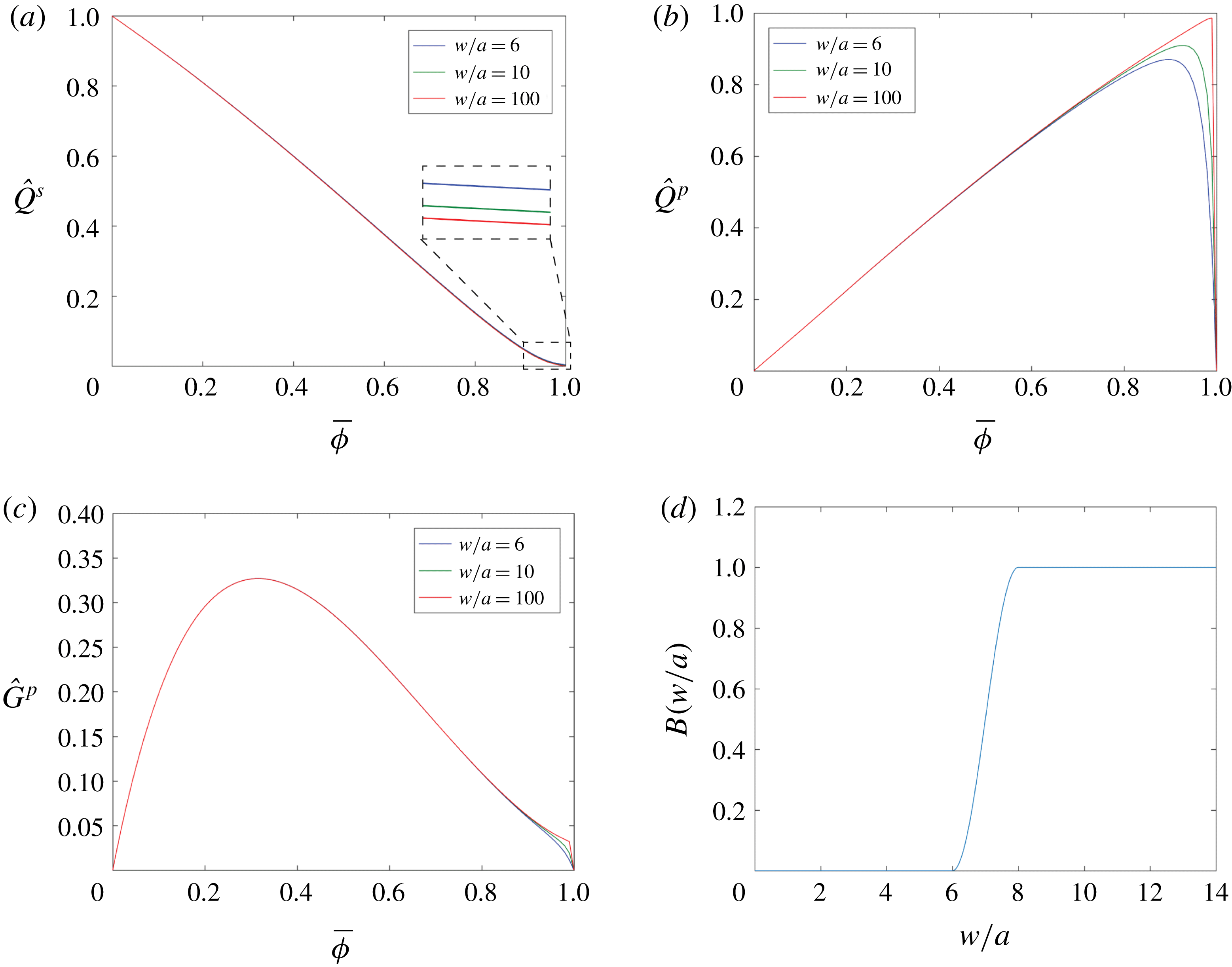
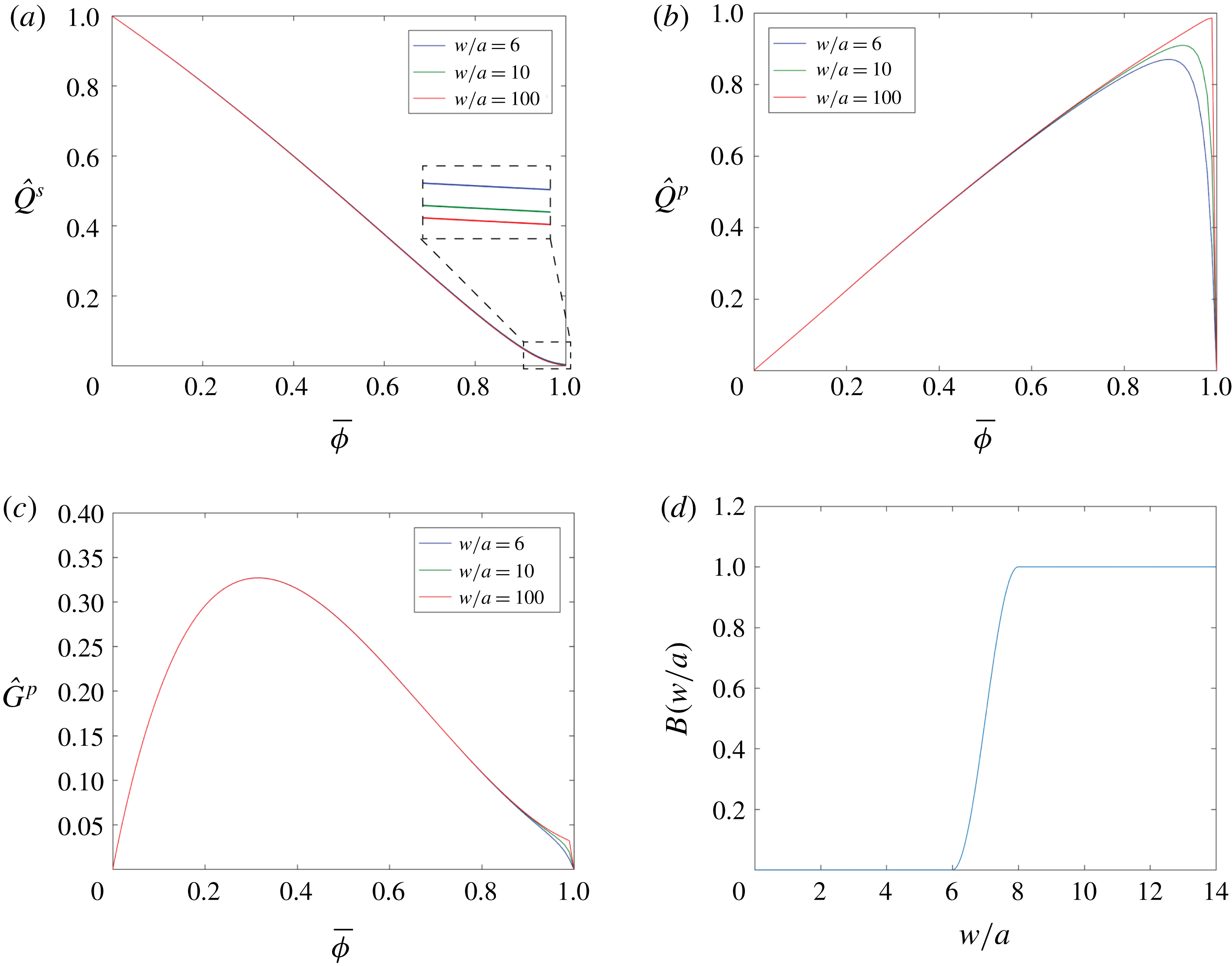
). The first term of (2.2) represents the reciprocal of the effective viscosity of the slurry. The slurry viscosity increases with an increase in the proppant concentration due to the interactions between particles and between particle and fluid. The second term of (2.2) accounts for Darcian flow within the porous medium. This term is trivial when proppant concentration is small and becomes significant when normalized proppant concentration is close to 1, as shown in figure 3(a). Thus, (2.3) is able to capture the transition from Poiseuille flow to Darcy filtration flow as the normalized proppant concentration increases from 0 to 1. Note that when
 $\bar{\unicode[STIX]{x1D719}}=0$
, i.e. before the proppant is introduced,
 $\hat{Q}^{s}=1$
and (2.3) recovers the fluid flow equation used in the classical PKN model.
The functions (a)
 $\hat{Q}^{s}$
, (b)
 $\hat{Q}^{p}$
and (c)
 ${\hat{G}}^{p}$
introduced by Dontsov & Peirce (Reference Dontsov and Peirce2014) versus normalized proppant concentration for three specified values of the parameter
 $w/a$
, and (d) the blocking function
 $B(w/a)$
versus the parameter
 $w/a$
when
 $N=3$
.
By considering fracture inflation, fluid flow and fluid leak-off, the local fluid mass balance equation can be written as
 $$\begin{eqnarray}\frac{\unicode[STIX]{x2202}\bar{w}(x,t)}{\unicode[STIX]{x2202}t}+\frac{\unicode[STIX]{x2202}\bar{q}^{s}(x,t)}{\unicode[STIX]{x2202}x}+\frac{2C_{l}}{\sqrt{t-\unicode[STIX]{x1D70F}(x)}}=0,\end{eqnarray}$$
where
 $\bar{w}(x,t)=(1/H)\int _{-H/2}^{H/2}w(x,z,t)\,\text{d}z$
and
 $\bar{q}^{s}(x,t)=(1/H)\int _{-H/2}^{H/2}q^{s}(x,z,t)\,\text{d}z$
are the average width and flux over the fracture height, respectively, the constant
 $C_{l}$
is the Carter leak-off coefficient, and
 $\unicode[STIX]{x1D70F}(x)$
is the time at which the fracture leading edge arrives at location
 $x$
.
The fracture-propagation model ((2.2), (2.3) and (2.5)) is complemented by the boundary conditions at the inlet and the fracture tip as
 $$\begin{eqnarray}\bar{q}^{s}(0,t)=Q_{0}/2H\quad \text{and}\quad \bar{w}(l,t)=0,\end{eqnarray}$$
where
 $Q_{0}$
is the injection rate. Together with the initial conditions given by a small time asymptotic solution (Kovalyshen & Detournay Reference Kovalyshen and Detournay2010) and the proppant concentration field
 $\bar{\unicode[STIX]{x1D719}}(x,z,t)$
obtained by the proppant-transport model to be discussed below, this set of equations is sufficient to determine the evolution of the fracture footprint defined by
 $l(t)$
and
 $H$
, and the field quantities
 $w(x,z,t)$
,
 $q^{s}(x,z,t)$
and
 $p(x,t)$
.
2.3 Proppant transport
The two-dimensional mass balance equation for the proppant is written as
 $$\begin{eqnarray}\frac{\unicode[STIX]{x2202}w(x,z,t)\bar{\unicode[STIX]{x1D719}}(x,z,t)}{\unicode[STIX]{x2202}t}+\frac{\unicode[STIX]{x2202}q_{x}^{p}(x,z,t)}{\unicode[STIX]{x2202}x}+\frac{\unicode[STIX]{x2202}q_{z}^{p}(x,z,t)}{\unicode[STIX]{x2202}z}=0,\end{eqnarray}$$
where
 $q_{x}^{p}$
and
 $q_{z}^{p}$
, respectively, represent the proppant flux in
 $x$
and
 $z$
directions. The fluxes can be defined as
 $$\begin{eqnarray}\displaystyle & \displaystyle q_{x}^{p}=B\left(\frac{w}{a}\right)\hat{Q}^{p}\left(\bar{\unicode[STIX]{x1D719}},\frac{w}{a}\right)q^{s}, & \displaystyle\end{eqnarray}$$
 $$\begin{eqnarray}\displaystyle & \displaystyle q_{z}^{p}=-B\left(\frac{w}{a}\right)\frac{a^{2}w}{12\unicode[STIX]{x1D707}_{f}}(\unicode[STIX]{x1D70C}_{p}-\unicode[STIX]{x1D70C}_{f})g{\hat{G}}^{p}\left(\bar{\unicode[STIX]{x1D719}},\frac{w}{a}\right), & \displaystyle\end{eqnarray}$$
where
 $\unicode[STIX]{x1D70C}_{p}$
and
 $\unicode[STIX]{x1D70C}_{f}$
are densities of proppant particle and clear fracturing fluid, respectively,
 $g$
is the gravitational acceleration,
 $B$
is a blocking function,
 $\hat{Q}^{p}$
and
 ${\hat{G}}^{p}$
are two dimensionless functions of the proppant concentration
 $\bar{\unicode[STIX]{x1D719}}$
and the ratio of
 $w/a$
(Dontsov & Peirce Reference Dontsov and Peirce2014).
The blocking function
 $B$
accounts for proppant bridging which occurs when the fracture width is only of the order of several diameters of the proppant particles. This is described as
 $$\begin{eqnarray}\displaystyle B\left(\frac{w}{a}\right) & = & \displaystyle \frac{1}{2}\text{H}\left(\frac{w}{2a}-N\right)\text{H}\left(N+1-\frac{w}{2a}\right)\left(1+\cos \left(\unicode[STIX]{x03C0}\left(N+1-\frac{w}{2a}\right)\right)\right)\nonumber\\ \displaystyle & & \displaystyle +\,\text{H}\left(\frac{w}{2a}-N-1\right),\end{eqnarray}$$
where
 $N$
is a multiple of the particle diameter, and
 $\text{H}$
represents the Heaviside step function. Proppant bridging occurs when the fracture aperture is smaller than
 $N$
times the proppant particle diameter. As an illustration, figure 3(d) shows the function
 $B$
versus
 $w/a$
when
 $N=3$
.
Similar to the function
 $\hat{Q}^{s}$
, functions
 $\hat{Q}^{p}$
and
 ${\hat{G}}^{p}$
also come from an empirical constitutive model (Dontsov & Peirce Reference Dontsov and Peirce2014) and are written, respectively, as
 $$\begin{eqnarray}\displaystyle & \displaystyle \hat{Q}^{p}\left(\bar{\unicode[STIX]{x1D719}},\frac{w}{a}\right)=\frac{w^{2}Q^{p}(\bar{\unicode[STIX]{x1D719}})}{w^{2}Q^{s}(\bar{\unicode[STIX]{x1D719}})+a^{2}\bar{\unicode[STIX]{x1D719}}D}, & \displaystyle\end{eqnarray}$$
 $$\begin{eqnarray}\displaystyle & \displaystyle {\hat{G}}^{p}\left(\bar{\unicode[STIX]{x1D719}},\frac{w}{a}\right)=G^{p}(\bar{\unicode[STIX]{x1D719}})-\frac{w^{2}G^{s}(\bar{\unicode[STIX]{x1D719}})Q^{p}(\bar{\unicode[STIX]{x1D719}})}{w^{2}Q^{s}(\bar{\unicode[STIX]{x1D719}})+a^{2}\bar{\unicode[STIX]{x1D719}}D}, & \displaystyle\end{eqnarray}$$
where
 $Q^{p}$
,
 $G^{p}$
and
 $G^{s}$
are dimensionless functions of normalized proppant concentration
 $\bar{\unicode[STIX]{x1D719}}$
only. The functions
 $\hat{Q}^{p}$
and
 ${\hat{G}}^{p}$
describe the pressure-driven proppant convection and proppant settling, respectively, and are illustrated in figures 3(b) and 3(c). It can be observed from figure 3(b) that
 $\hat{Q}^{p}$
enables the proppant to flow slightly faster, on average, than the slurry for small proppant concentrations. This is due to the propensity for particles naturally migrate from the fracture walls and to concentrate towards the fracture centre where the slurry exhibits a relatively larger velocity than the regions near fracture walls. Both
 $\hat{Q}^{p}$
and
 ${\hat{G}}^{p}$
become zero when normalized proppant concentration approaches 1, indicating that an immobile bed is formed.
2.4 Conductivity evolution of the closed hydraulic fractures
A model developed by Wang & Elsworth (Reference Wang and Elsworth2018) is used to follow the evolution of the fracture width and conductivity as the hydraulic pressure decreases at the conclusion of pumping. This model is capable of accommodating the mechanical response of proppant packs, closure of rough fracture surfaces, and proppant embedment into fracture walls. The conductivity of the closed, partially propped fracture is obtained by employing the cubic law and the Kozeny–Carman model (Kozeny Reference Kozeny1927; Carman Reference Carman1937). The flexural displacement of the unsupported spans of the fracture can be captured, resulting in some high-conductivity flow channels, as illustrated in figure 2. This model is summarized briefly as follows.
Based on linear elasticity, the residual width profile
 $w_{r}(x,z)$
and the net stress applied on the fracture walls
 $\unicode[STIX]{x1D70E}_{n}(x,z)$
can be related by an integral equation as
 $$\begin{eqnarray}\displaystyle w_{r}(x,z)=\frac{4}{\unicode[STIX]{x03C0}E^{\prime }}\int _{-H/2}^{H/2}\unicode[STIX]{x1D70E}_{n}(x,s)G(z,s)\,\text{d}s-2w_{e}(x,z), & & \displaystyle\end{eqnarray}$$
where
 $w_{e}(x,z)$
is the depth of proppant embedment multiplied by a factor of two accounting for the embedment into both walls of the fracture, and
 $G(z,s)$
is a singular elastic kernel expressed as (Tada, Paris & Irwin Reference Tada, Paris and Irwin2000)
 $$\begin{eqnarray}\displaystyle G(z,s)=\cosh ^{-1}\frac{H^{2}-4sz}{2H|z-s|}. & & \displaystyle\end{eqnarray}$$
Note that the integral in (2.13) has to be understood in the sense of a Cauchy principal value. The net stress applied on the fracture walls
 $\unicode[STIX]{x1D70E}_{n}(z)$
can be viewed as a superposition of far-field stress acting perpendicular to the plane of the fracture
 $\unicode[STIX]{x1D70E}_{h}$
, fluid pressure within the fracture
 $p_{f}(x,z)$
, back stress from the proppant pack
 $\unicode[STIX]{x1D70E}_{p}(x,z)$
, and back stress from the fracture asperities
 $\unicode[STIX]{x1D70E}_{a}(x,z)$
:
 $$\begin{eqnarray}\displaystyle \unicode[STIX]{x1D70E}_{n}(x,z)=p_{f}(x,z)+\unicode[STIX]{x1D70E}_{p}(x,z)+\unicode[STIX]{x1D70E}_{a}(x,z)-\unicode[STIX]{x1D70E}_{h}. & & \displaystyle\end{eqnarray}$$
Assuming that the proppant pack has a constant compressibility
 $c_{p}$
, the stress field driving compaction can be written as
 $$\begin{eqnarray}\displaystyle \unicode[STIX]{x1D70E}_{p}(x,z)=\left\{\begin{array}{@{}ll@{}}\displaystyle \frac{1}{c_{p}}\ln \frac{w_{r0}(x,z)\bar{\unicode[STIX]{x1D719}}_{r0}(x,z)}{w_{r}(x,z)},\quad & w_{r}(x,z)<w_{r0}(x,z)\bar{\unicode[STIX]{x1D719}}_{r0}(x,z)\\ 0,\quad & w_{r}(x,z)\geqslant w_{r0}(x,z)\bar{\unicode[STIX]{x1D719}}_{r0}(x,z),\end{array}\right. & & \displaystyle\end{eqnarray}$$
where
 $w_{r0}$
and
 $\bar{\unicode[STIX]{x1D719}}_{r0}$
are the fracture width and proppant concentration when pumping stops. They both have a subscript 0 because the conditions at the end of the pumping defines the initial conditions for the fracture closure analysis. The product of
 $w_{r0}$
and
 $\bar{\unicode[STIX]{x1D719}}_{r0}$
gives the initial width of the proppant pack.
For the unpropped fracture regions, roughness of fracture walls controls the closure of the two elastic surfaces in contact. The contact stress of the asperity can be described as (Bandis, Lumsden & Barton Reference Bandis, Lumsden and Barton1983; Barton, Bandis & Bakhtar Reference Barton, Bandis and Bakhtar1985)
 $$\begin{eqnarray}\unicode[STIX]{x1D70E}_{a}(x,z)=\left\{\begin{array}{@{}ll@{}}\displaystyle \frac{w_{a}-w_{r}(x,z)}{b_{1}-b_{2}[w_{a}-w_{r}(x,z)]},\quad & w_{r}(x,z)<w_{a}\\ 0,\quad & w_{r}(x,z)\geqslant w_{a},\end{array}\right.\end{eqnarray}$$
where
 $w_{a}$
is the asperity width,
 $b_{1}$
is a constant representing the compliance of the asperity, and
 $b_{2}=b_{1}/w_{a}$
. Note that this model gives
 $\unicode[STIX]{x1D70E}_{a}(x,z)=0$
at
 $w(x,z)\geqslant w_{a}$
and an infinite
 $\unicode[STIX]{x1D70E}_{a}(x,z)$
as
 $w(x,z)$
goes to zero, implying that the fracture is not allowed to completely close.
Based on the elastic Hertzian contact theory, the depth of proppant embedment can be written as
 $$\begin{eqnarray}w_{e}(x,z)=\left\{\begin{array}{@{}ll@{}}\displaystyle a\left(\frac{3\unicode[STIX]{x03C0}}{4E^{\prime }}\right)^{2}\left[\frac{16\unicode[STIX]{x1D702}{E^{\prime }}^{2}}{9\unicode[STIX]{x03C0}^{3}c_{p}}\ln \frac{w_{r0}(x,z)\bar{\unicode[STIX]{x1D719}}_{r0}(x,z)}{w_{r}(x,z)}\right]^{2/3},\quad & w_{r}(x,z)<w_{r0}(x,z)\bar{\unicode[STIX]{x1D719}}_{r0}(x,z)\\ 0,\quad & w_{r}(x,z)\geqslant w_{r0}(x,z)\bar{\unicode[STIX]{x1D719}}_{r0}(x,z),\end{array}\right.\end{eqnarray}$$
where
 $\unicode[STIX]{x1D702}\geqslant 2\sqrt{3}$
is a constant determined by the proppant packing.
Given the fluid pressure distribution within the fracture
 $p_{f}(x,z)$
, the residual profile of the fracture aperture
 $w_{r}(x,z)$
can be obtained by the integral equation, i.e. (2.13), combined with (2.14)–(2.18). Following this, the conductivity of the compacted proppant packs and the unpropped fracture regions can be obtained by the cubic law and the Kozeny–Carman model, respectively, as
 $$\begin{eqnarray}C(x,z)=\left\{\begin{array}{@{}ll@{}}\displaystyle \frac{w_{r}^{3}(x,z)}{12}\hat{Q}^{s}\left[\bar{\unicode[STIX]{x1D719}}_{r}(x,z),\frac{w_{r}(x,z)}{a}\right],\quad & w_{r}(x,z)\geqslant w_{r0}(x,z)\bar{\unicode[STIX]{x1D719}}_{r0}(x,z)\\ \displaystyle w_{r}(x,z)\frac{a^{2}}{45}\frac{\unicode[STIX]{x1D711}_{r}^{3}(x,z)}{[1-\unicode[STIX]{x1D711}_{r}(x,z)]^{2}},\quad & w_{r}(x,z)<w_{r0}(x,z)\bar{\unicode[STIX]{x1D719}}_{r0}(x,z),\end{array}\right.\end{eqnarray}$$
where
 $\bar{\unicode[STIX]{x1D719}}_{r}(x,z)=w_{r0}(x,z)\bar{\unicode[STIX]{x1D719}}_{r0}(x,z)/w_{r}(x,z)$
is the residual proppant concentration, and
 $\unicode[STIX]{x1D711}_{r}(x,z)=1-\bar{\unicode[STIX]{x1D719}}_{r}(x,z)\unicode[STIX]{x1D719}_{max}$
is the residual porosity of the proppant pack.
3 Numerical algorithm
The problem under consideration is split into two steps: (i) solve for the fracture propagation and proppant transport during the hydraulic fracturing treatment (§§ 2.2 and 2.3); and then (ii) solve for fracture closure to define the evolution of fracture conductivity after pumping ceases (§ 2.4), i.e. during shut-in, flowback and production stages, based on the fracture geometry and the proppant distribution obtained by step (i). The numerical algorithm for solving the fracture propagation and proppant transport is discussed in this section, with details of the fracture closure model (Wang & Elsworth Reference Wang and Elsworth2018) omitted here for brevity.
The two equation systems representing fracture propagation and proppant transport are coupled sequentially and solved in sequence, at each time step for (i) fracture propagation (2.2)–(2.6) then (ii) proppant transport (2.7)–(2.12). The fracture-propagation equations are first solved to obtain the fracture geometry (length and width profile) and the flow rate of the fluid/slurry, and the proppant-transport equations are then solved to update the proppant distribution within the fracture. In this scheme, each system is solved while holding the primary variable from another system of equations constant at each time step. We first introduce a moving mesh to facilitate the solution of the moving-boundary problem and then discuss the numerical algorithm for fracture propagation and proppant transport.
3.1 Moving mesh
The equation systems are defined over the range
 $0\leqslant x\leqslant l(t)$
which varies with the propagating fracture, forming a complex moving-boundary problem. In order to avoid adjusting the spatial discretization at each time step, a moving mesh is introduced to reformulate the equation systems for fracture propagation and proppant transport in terms of the moving coordinate defined as
 $$\begin{eqnarray}\unicode[STIX]{x1D709}=\frac{x}{l(t)},\quad 0\leqslant \unicode[STIX]{x1D709}\leqslant 1.\end{eqnarray}$$
The conversion of parameters from
 $x$
to
 $\unicode[STIX]{x1D709}$
requires a corresponding transformation of spatial and time derivatives written as
 $$\begin{eqnarray}\displaystyle & \displaystyle \left.\frac{\unicode[STIX]{x2202}(\cdot )}{\unicode[STIX]{x2202}t}\right|_{x}=\left.\frac{\unicode[STIX]{x2202}(\cdot )}{\unicode[STIX]{x2202}t}\right|_{\unicode[STIX]{x1D709}}-\unicode[STIX]{x1D709}\frac{\dot{l}}{l}\left.\frac{\unicode[STIX]{x2202}(\cdot )}{\unicode[STIX]{x2202}\unicode[STIX]{x1D709}}\right|_{t}, & \displaystyle\end{eqnarray}$$
 $$\begin{eqnarray}\displaystyle & \displaystyle \left.\frac{\unicode[STIX]{x2202}(\cdot )}{\unicode[STIX]{x2202}x}\right|_{t}=\frac{1}{l}\left.\frac{\unicode[STIX]{x2202}(\cdot )}{\unicode[STIX]{x2202}\unicode[STIX]{x1D709}}\right|_{t}, & \displaystyle\end{eqnarray}$$
where
 $\dot{l}=\text{d}l/\text{d}t$
is the velocity of fracture propagation. Under this transformation, Poiseuille’s law (2.3) and the governing equations for fluid/slurry flow (2.5) and proppant transport (2.7) can be rewritten, respectively, as
 $$\begin{eqnarray}\displaystyle & \displaystyle q^{s}=-\frac{w^{3}}{12\unicode[STIX]{x1D707}_{f}l}\hat{Q}^{s}\frac{\unicode[STIX]{x2202}p}{\unicode[STIX]{x2202}\unicode[STIX]{x1D709}}, & \displaystyle\end{eqnarray}$$
 $$\begin{eqnarray}\displaystyle & \displaystyle \frac{\unicode[STIX]{x2202}\bar{w}}{\unicode[STIX]{x2202}t}-\unicode[STIX]{x1D709}\frac{\dot{l}}{l}\frac{\unicode[STIX]{x2202}\bar{w}}{\unicode[STIX]{x2202}\unicode[STIX]{x1D709}}+\frac{1}{l}\frac{\unicode[STIX]{x2202}\bar{q}^{s}}{\unicode[STIX]{x2202}\unicode[STIX]{x1D709}}+\frac{2C_{l}}{\sqrt{t-\unicode[STIX]{x1D70F}(l\unicode[STIX]{x1D709})}}=0 & \displaystyle\end{eqnarray}$$
and
 $$\begin{eqnarray}\displaystyle \frac{\unicode[STIX]{x2202}w\bar{\unicode[STIX]{x1D719}}}{\unicode[STIX]{x2202}t}+\frac{\dot{l}}{l}w\bar{\unicode[STIX]{x1D719}}+\frac{1}{l}\frac{\unicode[STIX]{x2202}\tilde{q}_{x}^{p}}{\unicode[STIX]{x2202}\unicode[STIX]{x1D709}}+\frac{\unicode[STIX]{x2202}q_{z}^{p}}{\unicode[STIX]{x2202}z}=0, & & \displaystyle\end{eqnarray}$$
with
 $\tilde{q}_{x}^{p}=q_{x}^{p}-\unicode[STIX]{x1D709}\dot{l}w\bar{\unicode[STIX]{x1D719}}$
.
3.2 Numerical algorithm for fracture propagation
The equation system for fracture propagation is solved by a fourth-order collocation scheme similar to that used by Adachi, Detournay & Peirce (Reference Adachi, Detournay and Peirce2010). Combining (2.2) and (3.4) and taking the integral over fracture height gives
 $$\begin{eqnarray}\displaystyle \frac{\unicode[STIX]{x2202}\bar{w}}{\unicode[STIX]{x2202}\unicode[STIX]{x1D709}}=-\frac{\unicode[STIX]{x03C0}^{3}H\unicode[STIX]{x1D707}_{f}l}{2E^{\prime }\bar{w}^{3}\hat{Q}^{s}}\bar{q}^{s}=F_{1}(\unicode[STIX]{x1D709};\bar{w},\bar{q}^{s},l), & & \displaystyle\end{eqnarray}$$
enabling (3.5) to be written in the form
 $$\begin{eqnarray}\displaystyle \frac{\unicode[STIX]{x2202}\bar{q}^{s}}{\unicode[STIX]{x2202}\unicode[STIX]{x1D709}}=-l\dot{\bar{w}}-\unicode[STIX]{x1D709}\frac{\unicode[STIX]{x03C0}^{3}H\unicode[STIX]{x1D707}_{f}l\dot{l}}{2E^{\prime }\bar{w}^{3}\hat{Q}^{s}}\bar{q}^{s}-\frac{2C_{l}l}{\sqrt{t-\unicode[STIX]{x1D70F}(l\unicode[STIX]{x1D709})}}=F_{2}(\unicode[STIX]{x1D709};\bar{w},\bar{q}^{s},l), & & \displaystyle\end{eqnarray}$$
where
 $\hat{Q}^{s}$
is evaluated as
 $\hat{Q}^{s}(\bar{\unicode[STIX]{x1D719}}_{avg},\bar{w}/a)$
with
 $\bar{\unicode[STIX]{x1D719}}_{avg}$
being the averaged value of
 $\bar{\unicode[STIX]{x1D719}}$
over the fracture height, i.e.
 $\bar{\unicode[STIX]{x1D719}}_{avg}(\unicode[STIX]{x1D709},t)=(1/H)\int _{-H/2}^{H/2}w(\unicode[STIX]{x1D709},z,t)\,\text{d}z$
.
Integrating (3.5) in space over the length of the fracture and then in time over the total elapsed time yields the global mass balance equation
 $$\begin{eqnarray}\displaystyle \frac{Q_{0}}{2H}t=\int _{0}^{1}\bar{w}(\unicode[STIX]{x1D709},t)\,\text{d}\unicode[STIX]{x1D709}+4C_{l}\int _{0}^{1}\sqrt{t-\unicode[STIX]{x1D70F}(l\unicode[STIX]{x1D709})}\,\text{d}\unicode[STIX]{x1D709}. & & \displaystyle\end{eqnarray}$$
The time derivatives in (3.8) are approximated by a backward difference scheme as
 $$\begin{eqnarray}\displaystyle \dot{l}=\frac{l^{t}-l^{t-\unicode[STIX]{x0394}t}}{\unicode[STIX]{x0394}t}\quad \text{and}\quad \dot{\bar{w}}=\frac{\bar{w}^{t}-\bar{w}^{t-\unicode[STIX]{x0394}t}}{\unicode[STIX]{x0394}t}. & & \displaystyle\end{eqnarray}$$
The domain
 $0\leqslant \unicode[STIX]{x1D709}\leqslant 1$
is discretized into
 $n-1$
subintervals with
 $n$
points. Defining the vectors
 $Y=[\bar{w},\bar{q}^{s}]^{\text{T}}$
and
 $F=[F_{1},F_{2}]^{\text{T}}$
, the system of equations (3.7) and (3.8) can be rewritten in compact form as
 $$\begin{eqnarray}\displaystyle \frac{\,\text{d}Y^{t}}{\,\text{d}\unicode[STIX]{x1D709}}=F(\unicode[STIX]{x1D709};Y^{t},l^{t}). & & \displaystyle\end{eqnarray}$$
Taking the integral of (3.11) over a specific subinterval gives
 $$\begin{eqnarray}\displaystyle Y_{i+1}^{t}=Y_{i}^{t}+\frac{\unicode[STIX]{x0394}\unicode[STIX]{x1D709}}{6}(F_{i}^{t}+4F_{i+1/2}^{t}+F_{i+1}^{t}), & & \displaystyle\end{eqnarray}$$
where Simpson’s rule is used to approximate the integral in space. In (3.12), the term
 $F_{i+1/2}^{t}$
can be expressed as
 $$\begin{eqnarray}\displaystyle F_{i+1/2}^{t}=F(\unicode[STIX]{x1D709}_{i+1/2};Y_{i+1/2}^{t},l^{t}), & & \displaystyle\end{eqnarray}$$
where
 $Y_{i+1/2}$
is approximated by the following Hermite cubic approximation as
 $$\begin{eqnarray}\displaystyle Y_{i+1/2}^{t}\simeq (Y_{i}^{t}+Y_{i+1}^{t})/2-(\unicode[STIX]{x0394}\unicode[STIX]{x1D709}/8)(F_{i+1}^{t}-F_{i}^{t}). & & \displaystyle\end{eqnarray}$$
Similarly, the storage and leak-off integrals in (3.9) can also be approximated using the scheme introduced above.
The above discretization reduces the equation system of fracture propagation (3.7)–(3.9) into
 $2n-1$
nonlinear equations. Together with the two boundary conditions (2.6), they are sufficient to solve for the
 $2n+1$
unknowns
 $\{\bar{w}_{1},\ldots ,\bar{w}_{n};\bar{q}_{1}^{s},\ldots ,\bar{q}_{n}^{s};l\}$
at time
 $t$
given the values at time
 $t-\unicode[STIX]{x0394}t$
. Finally, the fracture width profile and the flow rate field can be restored from the average values by the relations
 $$\begin{eqnarray}\displaystyle & \displaystyle w(\unicode[STIX]{x1D709},z)=\frac{4}{\unicode[STIX]{x03C0}H}(H^{2}-4z^{2})^{1/2}\bar{w}(\unicode[STIX]{x1D709}), & \displaystyle\end{eqnarray}$$
 $$\begin{eqnarray}\displaystyle & \displaystyle q^{s}(\unicode[STIX]{x1D709},z)=\frac{16}{3\unicode[STIX]{x03C0}H}(H^{2}-4z^{2})^{3/2}\bar{q}^{s}(\unicode[STIX]{x1D709})\frac{\displaystyle \hat{Q}^{s}\left(\bar{\unicode[STIX]{x1D719}},\frac{w}{a}\right)}{\displaystyle \hat{Q}^{s}\left(\bar{\unicode[STIX]{x1D719}}_{avg},\frac{\bar{w}}{a}\right)}, & \displaystyle\end{eqnarray}$$
which are recovered from the assumption that the cross-section of the fracture is elliptical.
3.3 Numerical algorithm for proppant transport
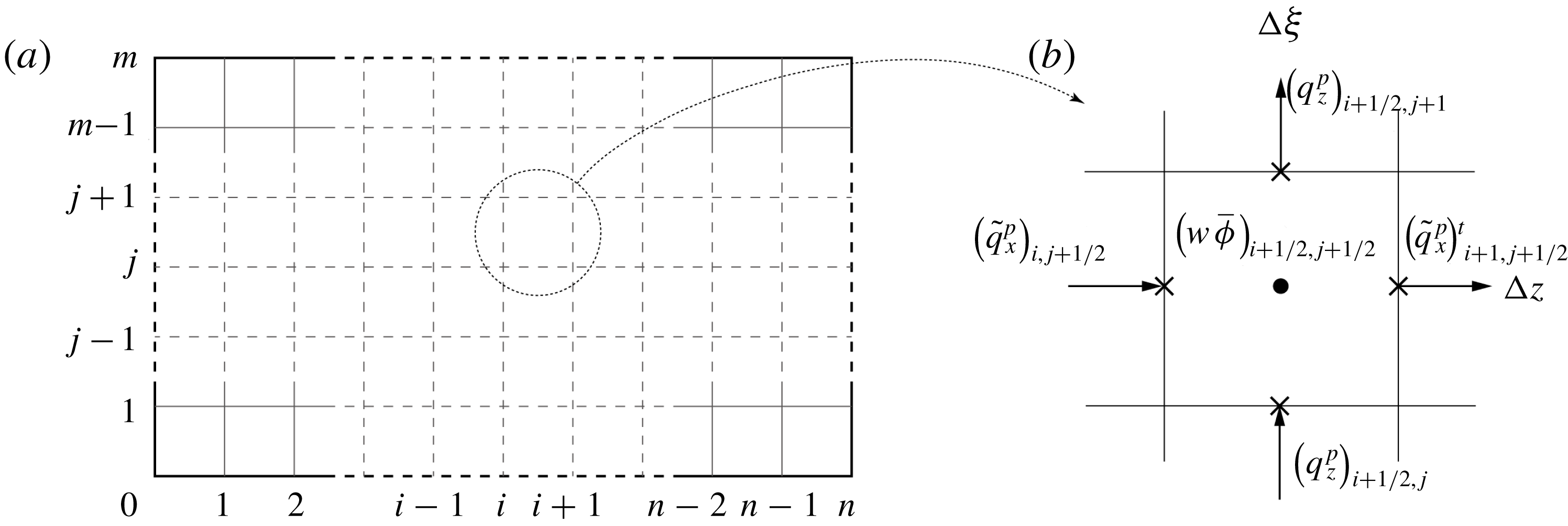
(a) Discretization of the problem domain for proppant transport. (b) Zoom-in of a specified element with the element centre and proppant fluxes marked.
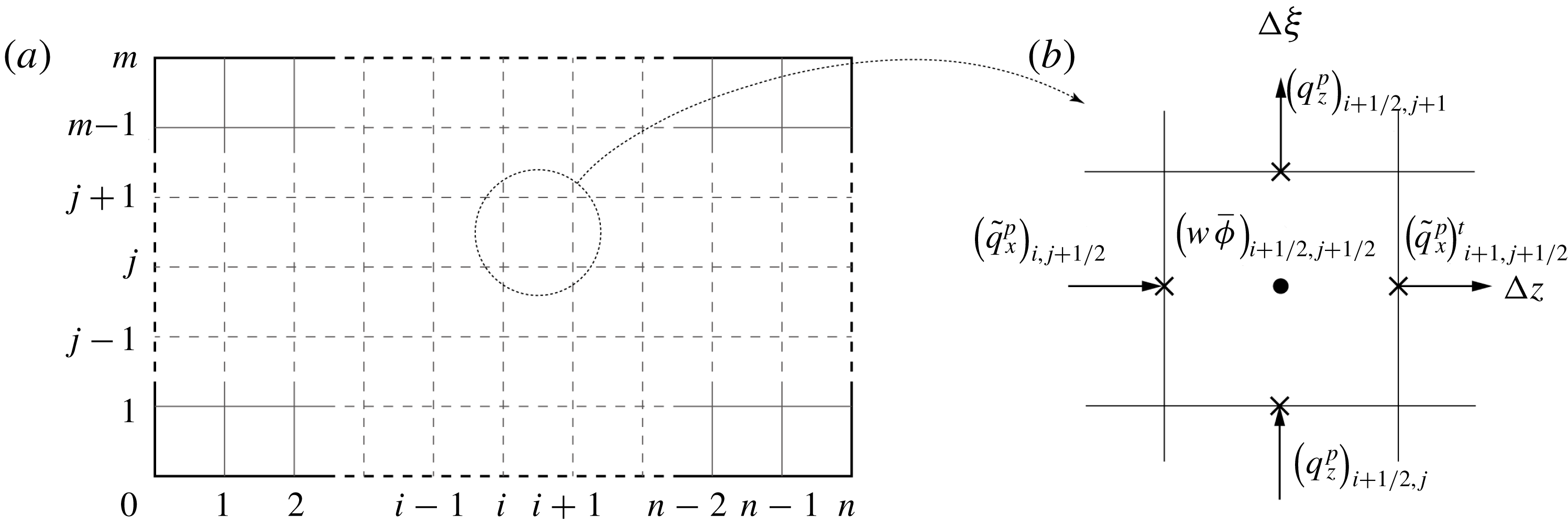
Proppant transport (i.e. (3.6)) is defined using a finite volume method with an explicit scheme advancing the solution in time. Discretization in the
 $\unicode[STIX]{x1D709}$
direction is consistent with that used in fracture propagation, and that for the
 $z$
direction, i.e.
 $-H/2\leqslant z\leqslant H/2$
, is discretized into
 $m-1$
subintervals. Thus, the problem domain is discretized into
 $(n-1)\times (m-1)$
rectangular elements of uniform size, as shown in figure 4(a). For a specific element (figure 4
b), equation (3.6) is discretized as
 $$\begin{eqnarray}\displaystyle (w\bar{\unicode[STIX]{x1D719}})_{i+1/2,j+1/2}^{t+\unicode[STIX]{x0394}t} & = & \displaystyle (w\bar{\unicode[STIX]{x1D719}})_{i+1/2,j+1/2}^{t}+\frac{\dot{l}\unicode[STIX]{x0394}t}{l}(w\bar{\unicode[STIX]{x1D719}})_{i+1/2,j+1/2}^{t}+\frac{\unicode[STIX]{x0394}t}{l\unicode[STIX]{x0394}\unicode[STIX]{x1D709}}\left[(\tilde{q}_{x}^{p})_{i,j+1/2}^{t}-(\tilde{q}_{x}^{p})_{i+1,j+1/2}^{t}\right]\nonumber\\ \displaystyle & & \displaystyle +\,\frac{\unicode[STIX]{x0394}t}{\unicode[STIX]{x0394}z}\left[(q_{z}^{p})_{i+1/2,j}^{t}-(q_{z}^{p})_{i+1/2,j+1}^{t}\right],\end{eqnarray}$$
where
 $(w\bar{\unicode[STIX]{x1D719}})_{i+1/2,j+1/2}=(w_{i,j+1/2}+w_{i+1,j+1/2})\bar{\unicode[STIX]{x1D719}}_{i+1/2,j+1/2}/2$
is defined at the centre of each element, and the fluxes
 $\tilde{q}_{x}^{p}$
and
 $q_{z}^{p}$
are defined at the centres of the element faces. An upwind scheme is used to calculate
 $\tilde{q}_{x}^{p}$
and
 $q_{z}^{p}$
through the element faces, i.e. the fluxes are calculated using the values from the centres of the adjacent elements upstream/upwind of the element under consideration. The sign of the ‘wind’ for
 $\tilde{q}_{x}^{p}$
and
 $q_{z}^{p}$
of each element can be determined, respectively, as
 $$\begin{eqnarray}\displaystyle & \displaystyle d_{x}=B\left(\frac{w}{a}\right)q_{x}^{s}\frac{\unicode[STIX]{x2202}}{\unicode[STIX]{x2202}\bar{\unicode[STIX]{x1D719}}}\hat{Q}^{p}\left(\bar{\unicode[STIX]{x1D719}},\frac{\bar{w}}{a}\right)-\dot{l}\unicode[STIX]{x1D709}, & \displaystyle\end{eqnarray}$$
 $$\begin{eqnarray}\displaystyle & \displaystyle d_{z}=-B\left(\frac{w}{a}\right)\frac{a^{2}}{12\unicode[STIX]{x1D707}^{f}}(\unicode[STIX]{x1D70C}^{p}-\unicode[STIX]{x1D70C}^{f})g\frac{\unicode[STIX]{x2202}}{\unicode[STIX]{x2202}\bar{\unicode[STIX]{x1D719}}}{\hat{G}}^{p}\left(\bar{\unicode[STIX]{x1D719}},\frac{w}{a}\right), & \displaystyle\end{eqnarray}$$
where all the values are from the centres of the elements. When the ‘winds’ of the two adjacent elements of an element face have the same sign, it is straightforward to apply the upwind scheme. However, when the two ‘winds’ exhibit opposite signs, the proppant flux
 $\tilde{q}_{x}^{p}$
or
 $q_{z}^{p}$
through this face should be chosen as the smaller of the two fluxes of the two adjacent elements. This treatment of winding should be implemented appropriately to achieve a numerically stable scheme and avoid the physically unrealistic solution where normalized proppant concentration
 $\bar{\unicode[STIX]{x1D719}}$
is elevated above 1.
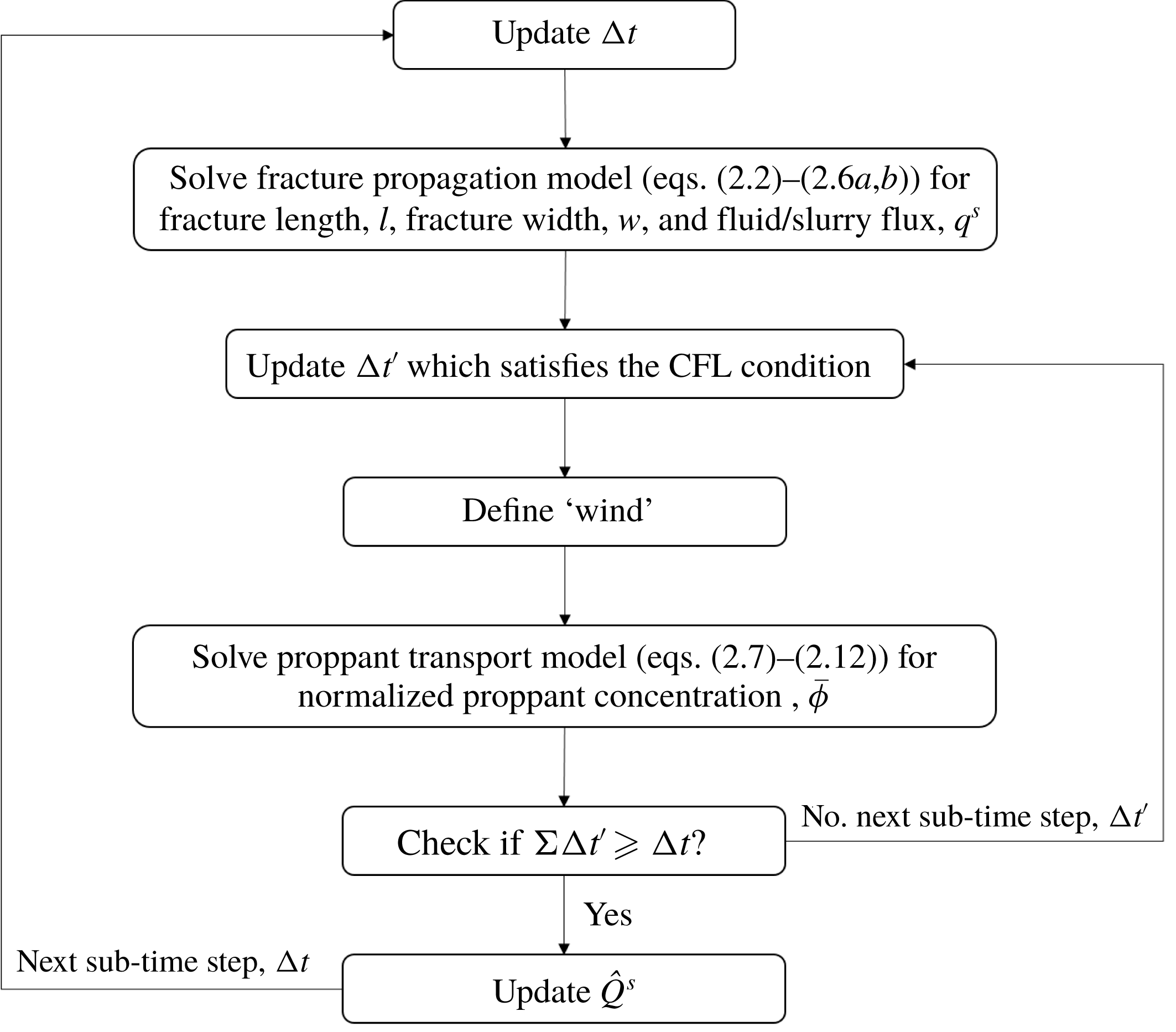
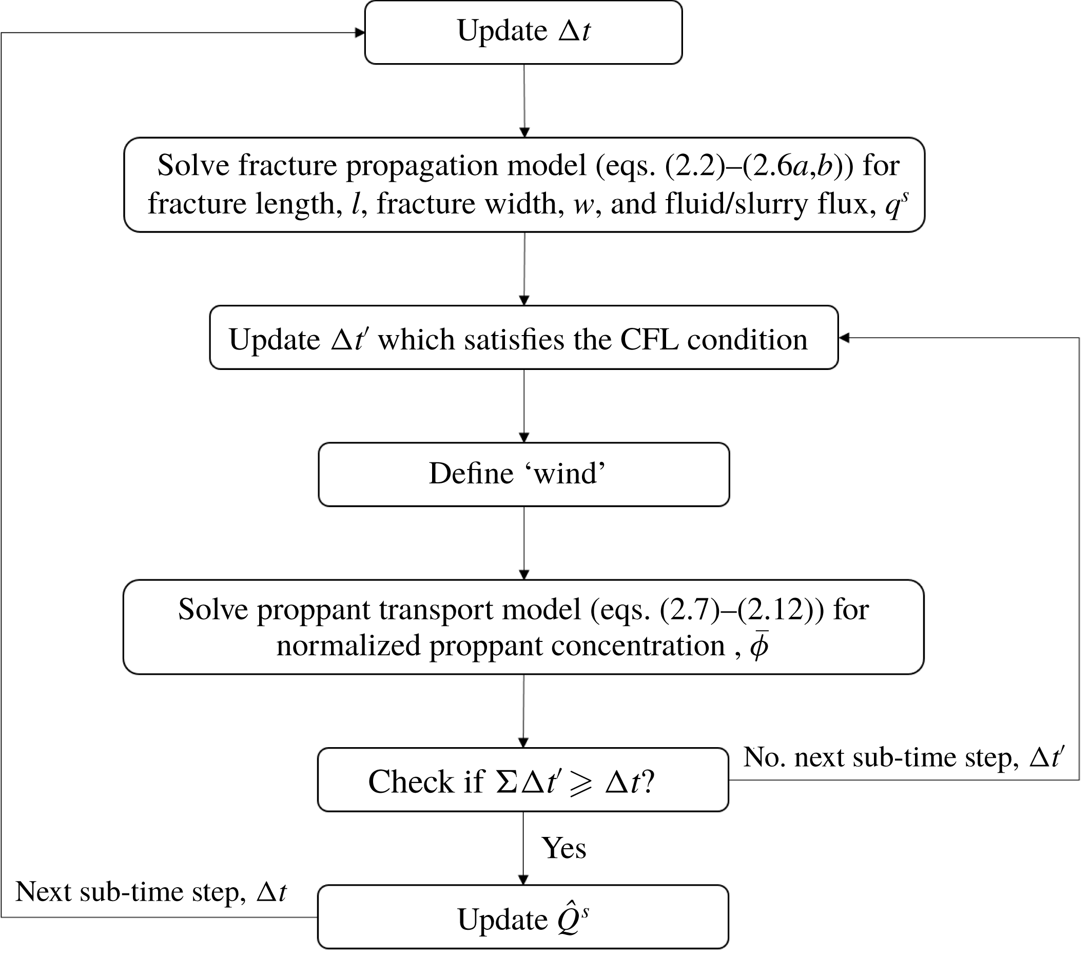
As indicated earlier, the equation system for fracture propagation is solved first to obtain the fracture geometry and the fluid flow field – this is then used to define proppant transport and to update the proppant distribution within the fracture. Since an implicit scheme is used, there is no restriction on the time step for solving the fracture propagation. However, an explicit scheme is employed for proppant transport, and this requires that the time step for the proppant transport should be small enough to satisfy the Courant–Friedrichs–Lewy (CFL) condition. In this numerical algorithm, a large time step
 $\unicode[STIX]{x0394}t$
is used when solving fracture propagation, and then is subdivided into smaller time steps
 $\unicode[STIX]{x0394}t^{\prime }$
, each of which satisfies the CFL condition, when solving for proppant transport. The procedure for this coupling process during a single time step is shown in figure 5.
Procedure for the modelling of fracture propagation and proppant transport during a single time step.
4 Results and discussion
In this section, we first validate the proposed model against a suitable previous study. Then, we describe a series of simulations of fracture propagation and proppant transport (§ 4.2). This includes a base case and several parametric studies to examine the effect of viscosity of fracturing fluid, proppant density, proppant size, and leak-off rate on the resulting fracture geometry and proppant distribution. Based on these results, fracture closure is represented to explore the role of proppant distribution on fracture conductivity (§ 4.3). Finally, we perform a series of reservoir simulations to visualize fluid flow patterns within the fractures during production and predict the gas production rate (§ 4.4), based on the estimates of spatially heterogeneous fracture conductivities.
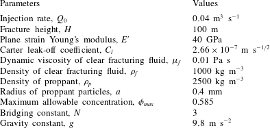
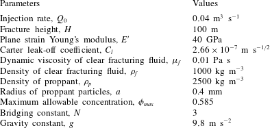
Parameters used in the validation simulation.
4.1 Model validation
The established fracture-propagation model (without proppant transport) has been benchmarked against both small and large time asymptotic solutions by Wang, Elsworth & Denison (Reference Wang, Elsworth and Denison2018a
), while the fracture-deflation model has shown excellent agreement with a published model (Wang & Elsworth Reference Wang and Elsworth2018). In this subsection, the model is further validated against a published result from Shiozawa & McClure (Reference Shiozawa and McClure2016), where both fracture propagation and proppant transport are simulated. The validation simulation was performed with the same input parameters as those in Shiozawa & McClure (Reference Shiozawa and McClure2016), as listed in table 1. For the pumping schedule, a pad of clean fluid is first injected for 2000 s, and then slurry is injected for a further 2000 s with a normalized proppant concentration
 $\bar{\unicode[STIX]{x1D719}}=0.2$
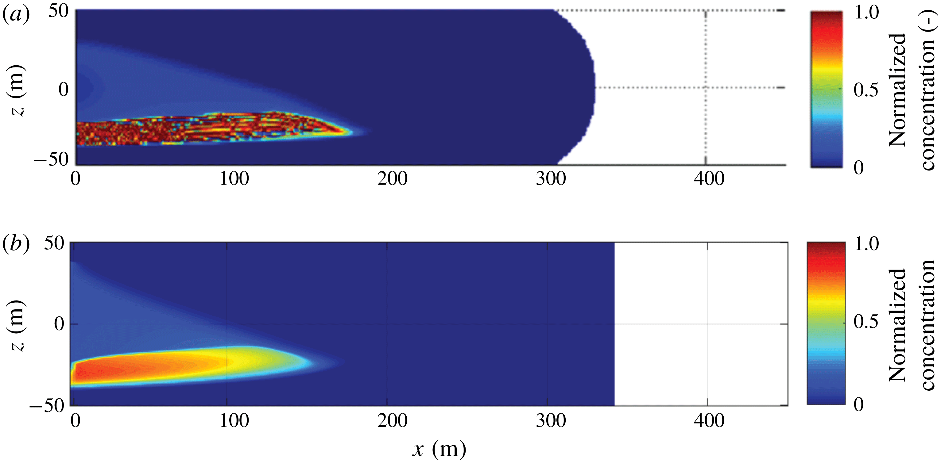
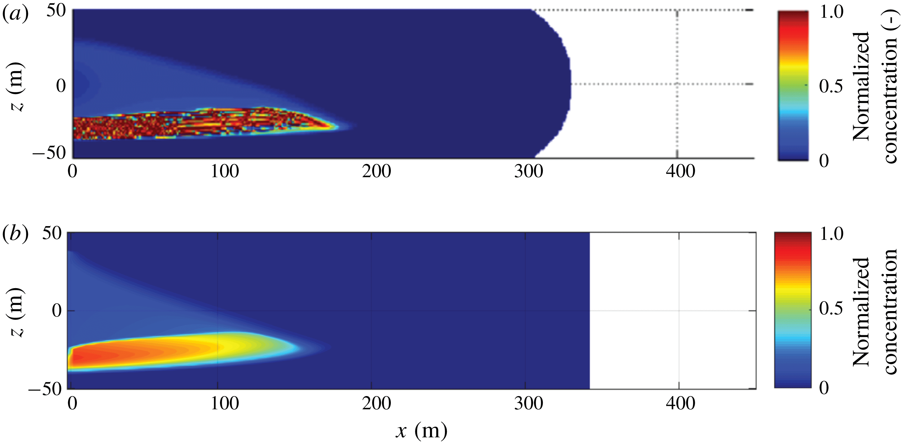
. Note that this pumping schedule is slightly different from that in Shiozawa & McClure (Reference Shiozawa and McClure2016), aiming to eliminate the influence of wellbore calculations conducted in Shiozawa & McClure (Reference Shiozawa and McClure2016) and ensure that the same amounts of fluid and proppant enter into the hydraulic fracture. The simulation results of the proposed model show good agreement with the published results, as shown in figure 6. It can be seen that, at the end of pumping (
 $t=4000~\text{s}$
), both of these two models show fracture lengths of
 ${\sim}340~\text{m}$
, normalized proppant concentrations in the suspension of
 ${\sim}0.2$
, and similar shapes of the settled proppant bank.
Comparison of fracture geometry and proppant distribution at
 $t=4000~\text{s}$
between (a) the published results from Shiozawa & McClure (Reference Shiozawa and McClure2016) and (b) the proposed model.
4.2 Results of fracture propagation and proppant transport
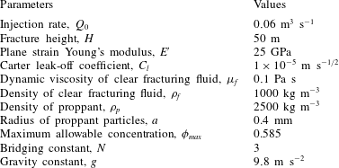
First, a base case is computed to evaluate fracture propagation and proppant transport (case 1). The input parameters are shown in table 2. The fracture is driven by the introduction of a clear fracturing fluid until
 $t=1000~\text{s}$
, and thereafter proppant is introduced to form a mixture of fracturing fluid and proppant particles. The injection rate is a constant
 $Q_{0}=0.06~\text{m}^{3}~\text{s}^{-1}$
, with the normalized proppant concentration of the injected slurry
 $\bar{\unicode[STIX]{x1D719}}=0.2$
. Simulation is ended at
 $t=2000~\text{s}$
when pumping stops.
Parameters used in the base case simulation.
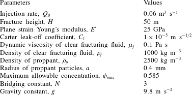
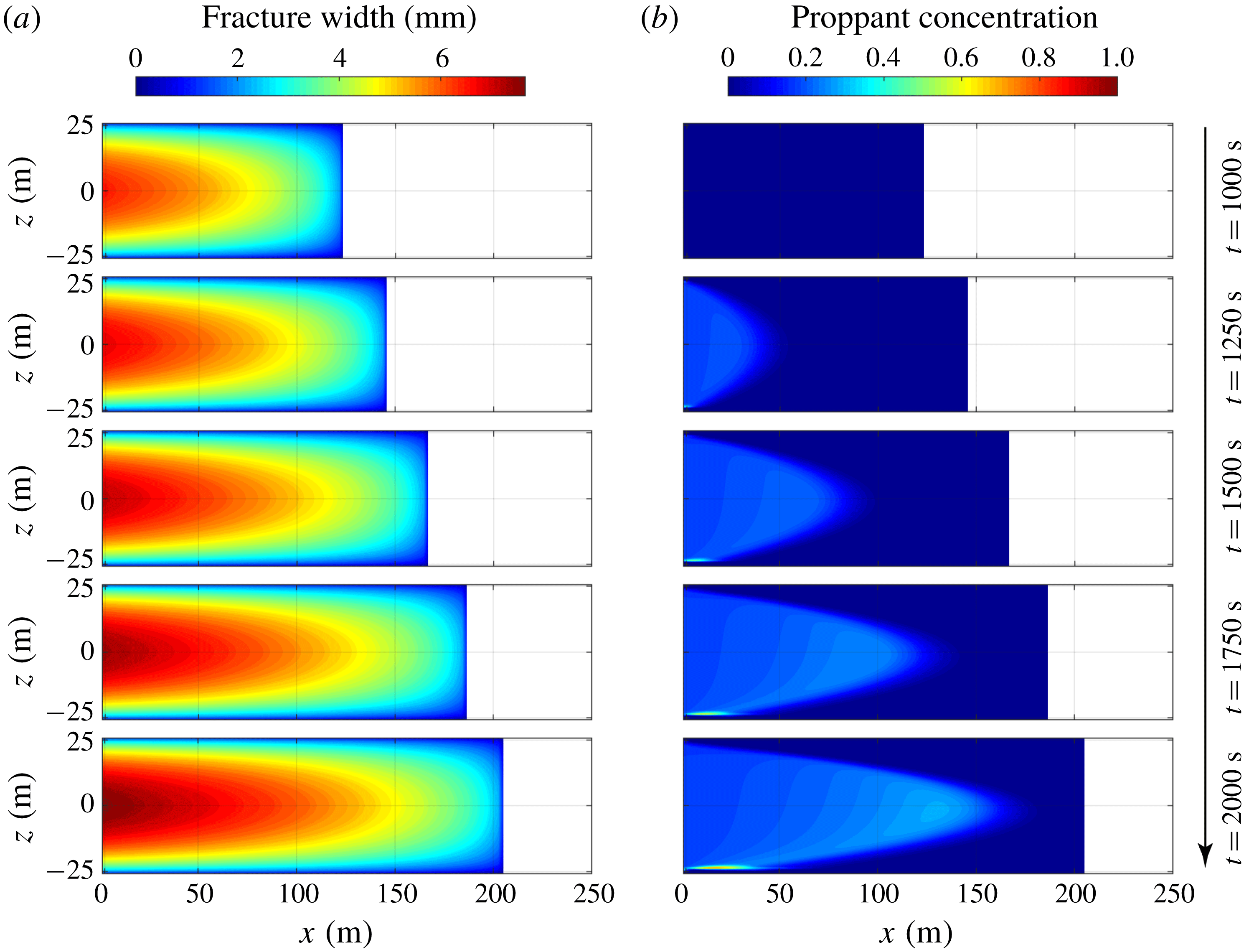
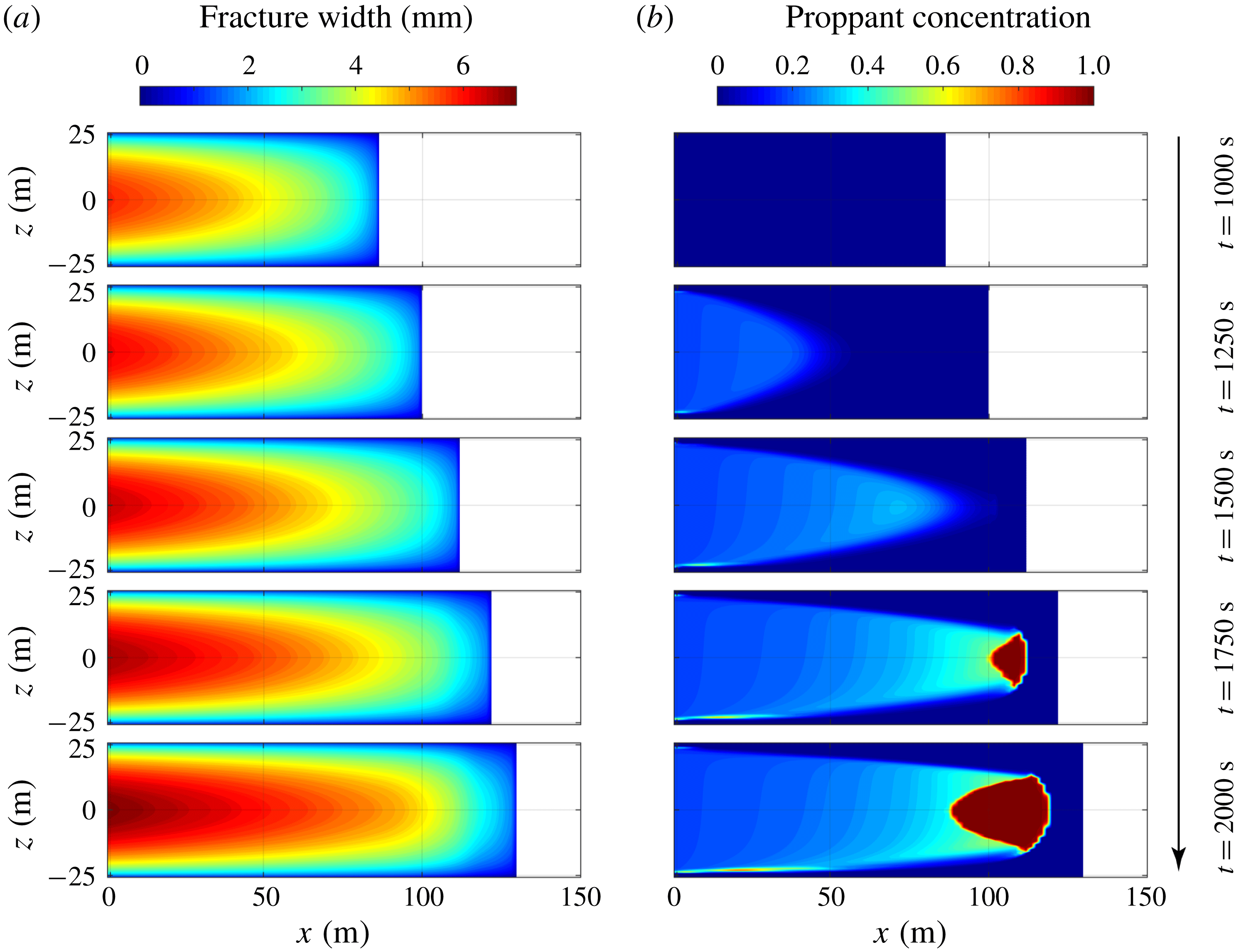
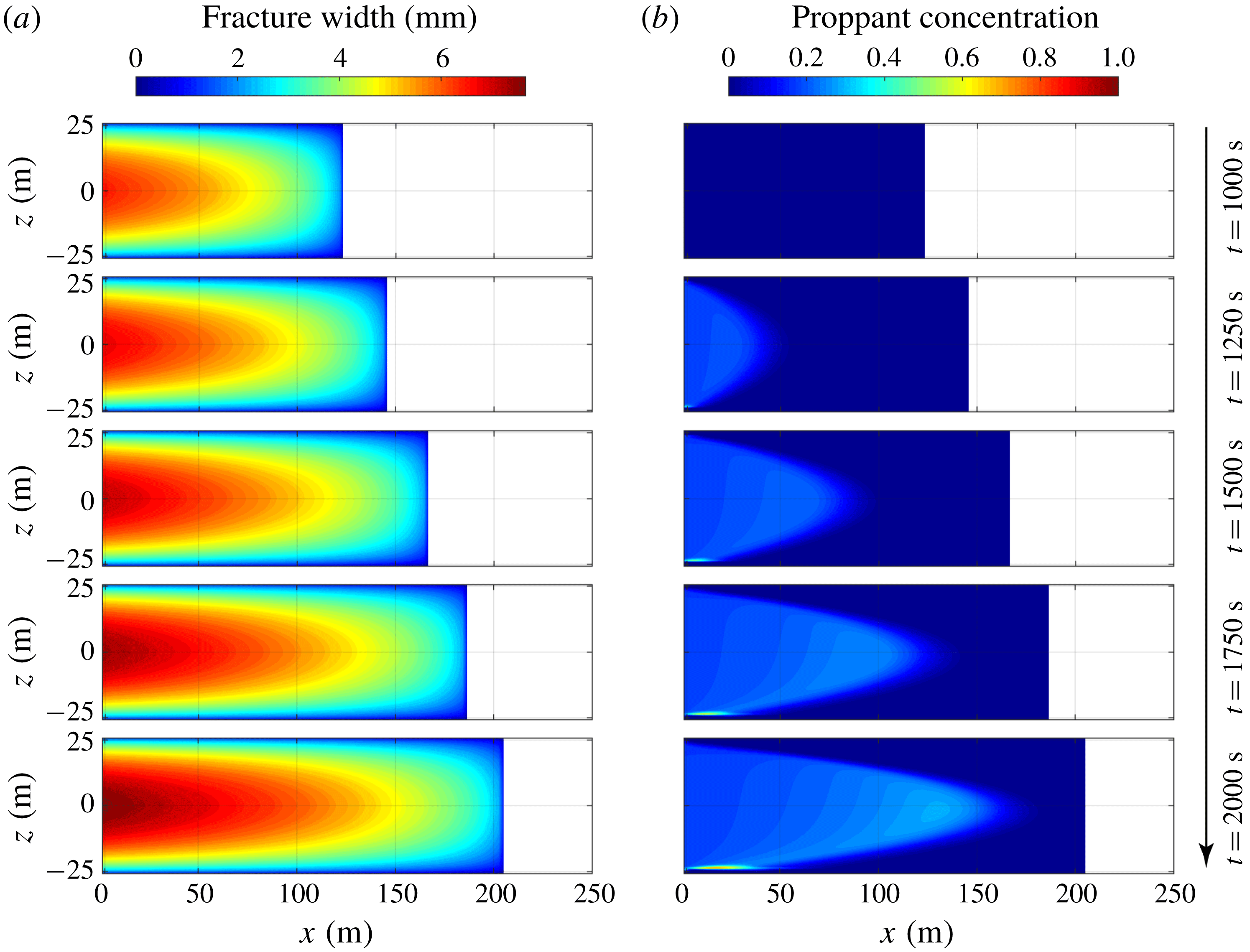
Figure 7 shows the fracture geometries (fracture lengths and aperture profiles) and corresponding proppant distribution at different snapshots in time at
 $t=1000~\text{s}$
,
 $t=1250~\text{s}$
,
 $t=1500~\text{s}$
,
 $t=1750~\text{s}$
and
 $t=2000~\text{s}$
. A symmetric bi-wing fracture is formed, but only one wing is modelled and shown. After 1000 s of injection of clear fracturing fluid, the fracture propagates to a half-length of
 ${\sim}122~\text{m}$
. Fracture apertures are greater in the central region of the fracture than the region close to the fracture edge, and reach a maximum value of
 ${\sim}6~\text{mm}$
at the wellbore (
 $x=0,z=0$
). At this point, since proppant has not been injected, the proppant concentration within the fracture is null. Following this, proppant is introduced and transported from the wellbore to fracture tip. It can be seen from figure 7(b) that the proppant distribution within the fracture is ‘triangular’ in its distribution and the proppant travels the fastest at mid-height of the fracture (
 $z=0$
). This is due to the largest aperture being present at
 $z=0$
(figure 7
a), resulting in the maximum flow rate. A proppant bank accumulates at the base of the fracture due to gravitational settling of the proppant; however, due to the high viscosity of the fracturing fluid, the settling velocity is small and the settling flux is minor (2.9) – as a result, the proppant bank is of limited size and the proppant distribution is relatively uniform. At the conclusion of pumping, i.e. when
 $t=2000~\text{s}$
, the fracture has a maximum half-length of
 ${\sim}205~\text{m}$
, and the proppant penetrates to
 $x\approx 170~\text{m}$
. This indicates that proppant travels
 ${\sim}2$
times faster than the rate of fracture propagation in this case, which results from both (i) fluid leak-off into the surrounding formation and (ii) the propensity for proppant to travel along the fracture centreline at a velocity in excess of the average fluid velocity.
Simulation results of the base case at different snapshots in time
 $t=1000~\text{s}$
,
 $t=1250~\text{s}$
,
 $t=1500~\text{s}$
,
 $t=1750~\text{s}$
and
 $t=2000~\text{s}$
: (a) fracture geometry and (b) proppant distribution.
It is beneficial to introduce a characteristic time for settling to estimate the time the proppant takes to settle from
 $z=0$
to
 $z=-H/2$
. Aided by (2.9) and the asymptotic behaviour of the function
 ${\hat{G}}^{p}$
(Dontsov & Peirce Reference Dontsov and Peirce2014), the characteristic settling time can be calculated as
 $$\begin{eqnarray}\displaystyle t_{s}=\frac{H}{2v_{settling}}=\frac{9H\unicode[STIX]{x1D707}_{f}}{4a^{2}(\unicode[STIX]{x1D70C}_{p}-\unicode[STIX]{x1D70C}_{f})g}. & & \displaystyle\end{eqnarray}$$
Thus, the ratio between the duration of proppant injection and the characteristic settling time can be used to predict whether the proppant will settle from its average location at mid-height to the base of the fracture at the conclusion of pumping, and is expressed as
 $$\begin{eqnarray}\displaystyle S=\frac{t_{PID}}{t_{s}}=\frac{4a^{2}(\unicode[STIX]{x1D70C}_{p}-\unicode[STIX]{x1D70C}_{f})gt_{PID}}{9H\unicode[STIX]{x1D707}_{f}}, & & \displaystyle\end{eqnarray}$$
where
 $t_{PID}$
is the duration of proppant injection, and
 $t_{PID}=1000~\text{s}$
for all cases in this study. If the dimensionless parameter
 $S\gg 1$
, the proppant will settle to the fracture base before pumping stops, while if
 $S\ll 1$
, a relatively uniform proppant distribution is expected at the end of the pumping. For the base case this ratio is
 $S=0.21$
.
In the following, four parametric studies were performed by changing fluid viscosity, proppant size, proppant density and leak-off coefficient, followed by a case to mimic conventional slick-water fracturing. In these five cases, the input parameters and pumping schedule are assumed to be consistent with those in the base case, except for the individual parameters that are directly specified.
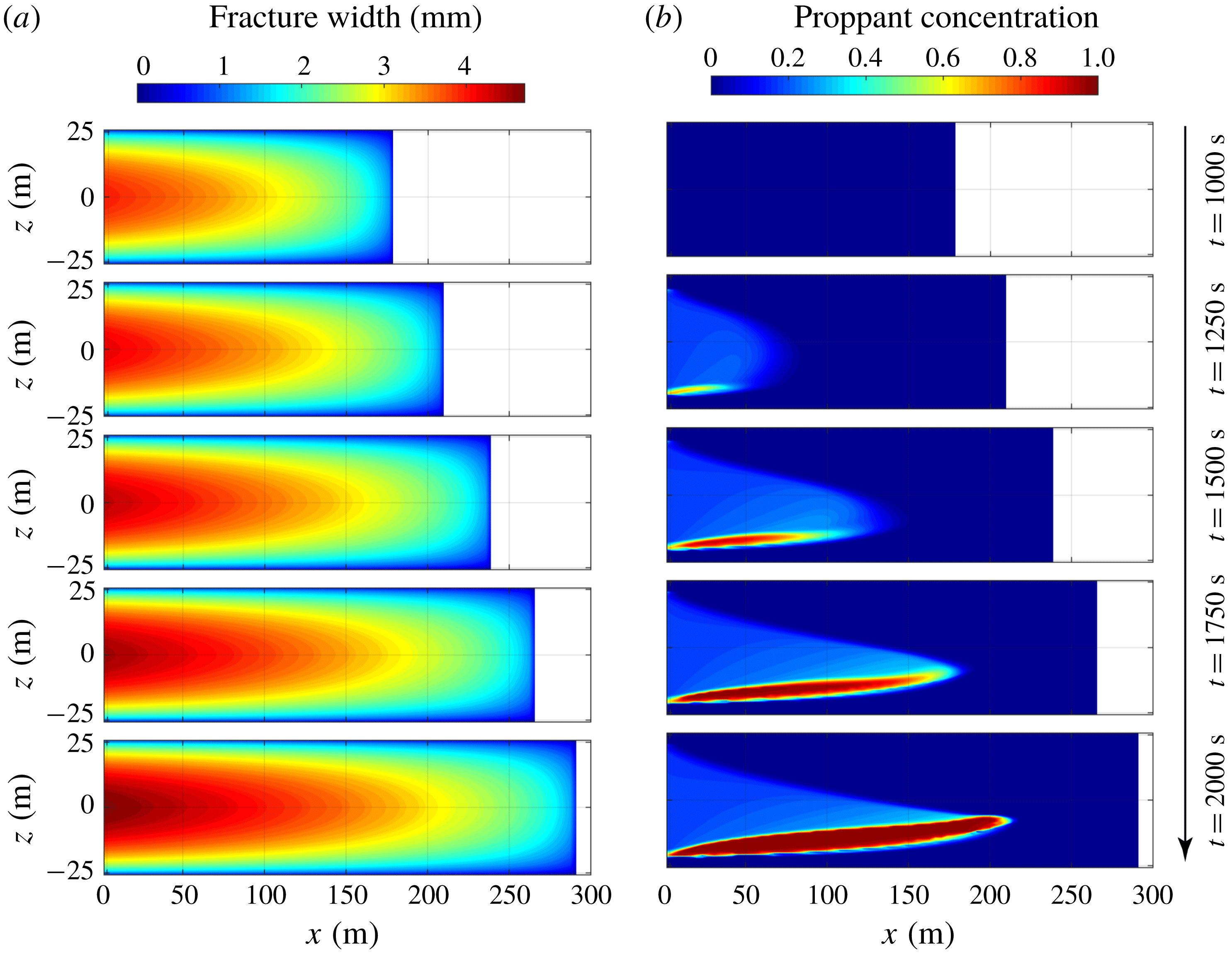
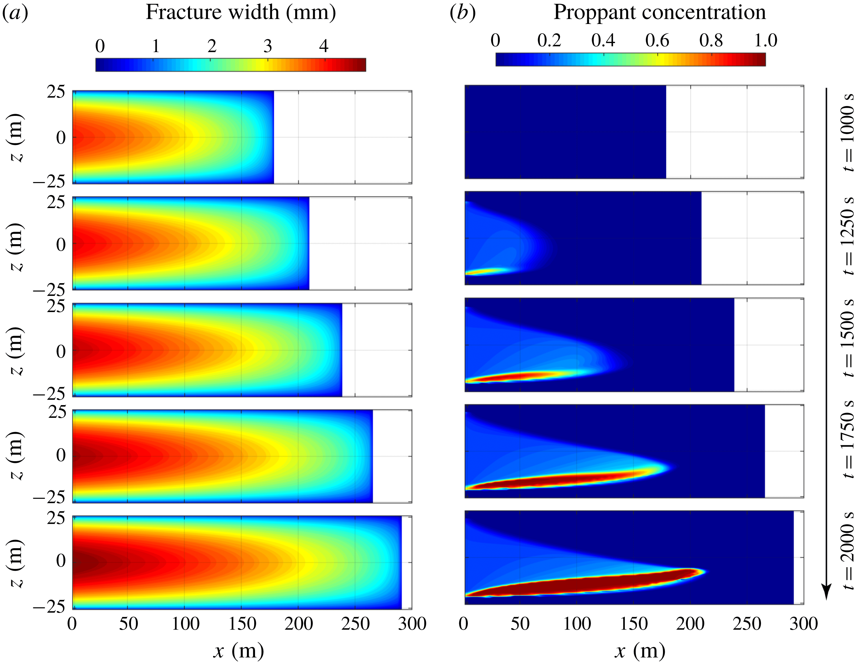
Simulation results of the case with low fluid viscosity (
 $\unicode[STIX]{x1D707}_{f}=0.01~\text{Pa}~\text{s}$
) at different snapshots in time
 $t=1000~\text{s}$
,
 $t=1250~\text{s}$
,
 $t=1500~\text{s}$
,
 $t=1750~\text{s}$
and
 $t=2000~\text{s}$
: (a) fracture geometry and (b) proppant distribution.
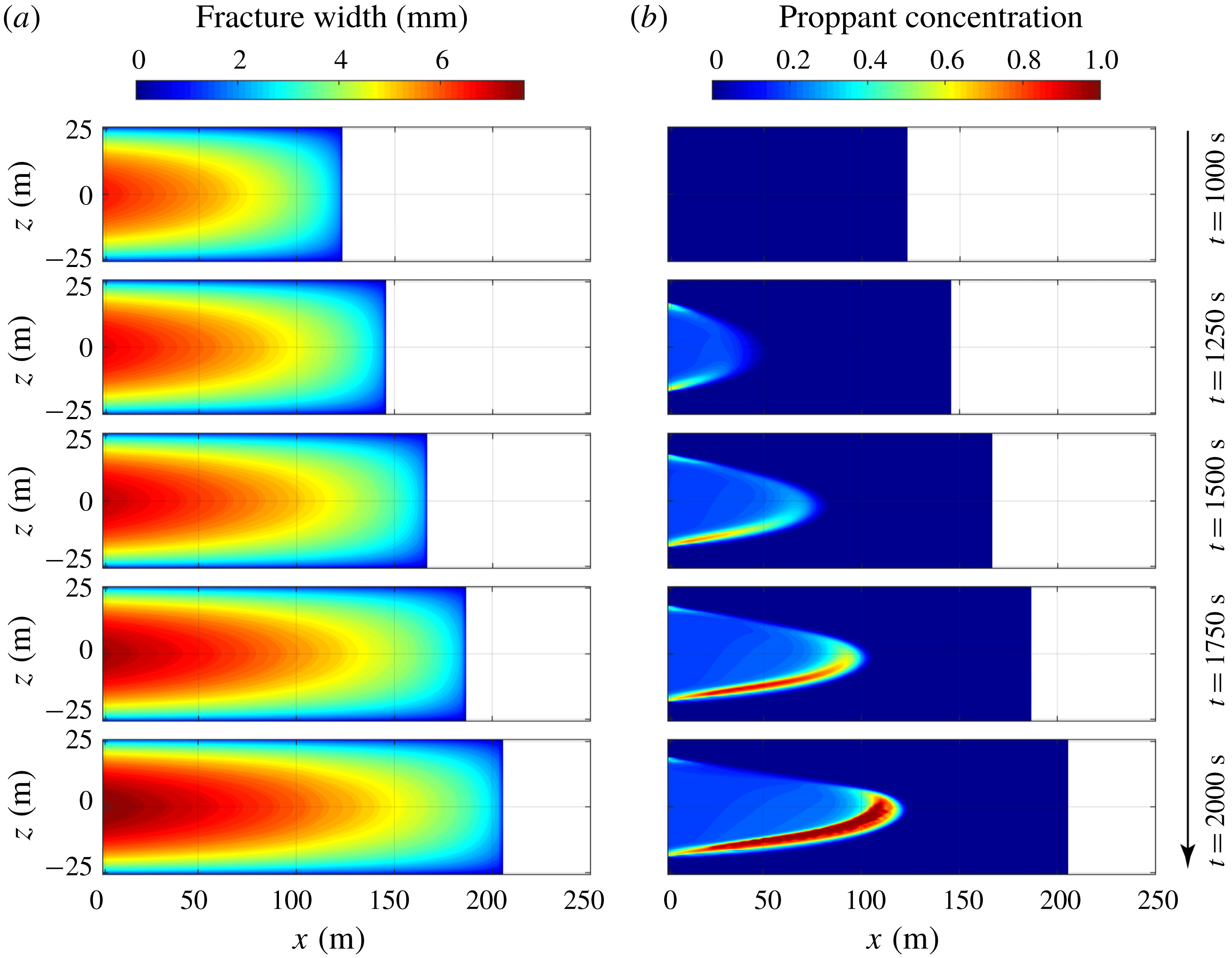
Simulation results of the case with large proppant size (
 $a=0.8~\text{mm}$
) at different snapshots in time
 $t=1000~\text{s}$
,
 $t=1250~\text{s}$
,
 $t=1500~\text{s}$
,
 $t=1750~\text{s}$
and
 $t=2000~\text{s}$
: (a) fracture geometry and (b) proppant distribution.
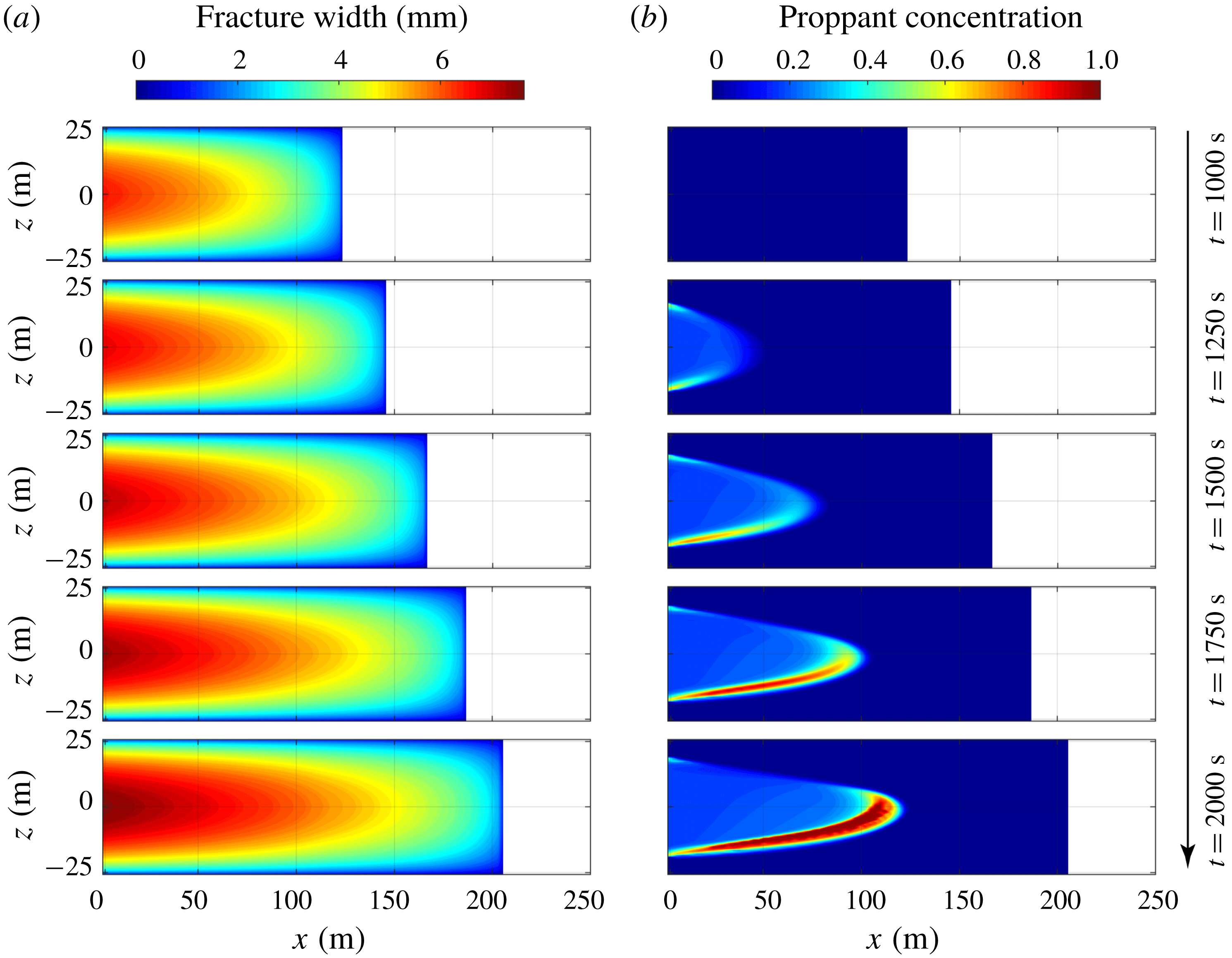
Figure 8 shows the simulation results for the case with a low fluid viscosity (case 2). In this case, the dynamic viscosity of the fracturing fluid is reduced to
 $\unicode[STIX]{x1D707}_{f}=0.01~\text{Pa}~\text{s}$
, which is one order of magnitude less than that used in the base case. Note that the leak-off coefficient in this case is assumed to be the same as the one used in the base case. Low fluid viscosity results in a longer fracture, which is
 ${\sim}290~\text{m}$
at the conclusion of pumping, but is represented by a smaller fracture aperture whose maximum value, when pumping stops, is only
 ${\sim}4.6~\text{mm}$
(figure 8
a). As can be seen from figure 8(b), due to the reduced fluid viscosity, proppant settles rapidly from suspension and accumulates in an immobile proppant bank at the fracture base – this is consistent with the dimensionless parameter
 $S\approx 2.10$
calculated by (4.2). However, the proppant does not settle completely to the base of the fracture, because proppant bridges form and the proppant becomes immobile when the fracture is too narrow.
Figure 9 shows results for the case with a large proppant size (case 3) where the particle radius is set to
 $a=0.8~\text{mm}$
. Apparent from figure 9(a) is that the larger proppant size does not significantly influence fracture propagation, with the resulting fracture geometry almost identical to that in the base case. Proppant settling is accelerated by the larger proppant size, as suggested by the value of
 $S\approx 0.84$
. Meanwhile, proppant bridges form beyond the half-length of the fracture where fracture aperture is less than three times the particle diameter. As a result, compared with the base case, the penetration of the proppant within the fracture, and therefore into the reservoir, is limited to much shorter distances from the borehole (
 ${\sim}120~\text{m}$
) at the conclusion of the pumping (figure 9
b).
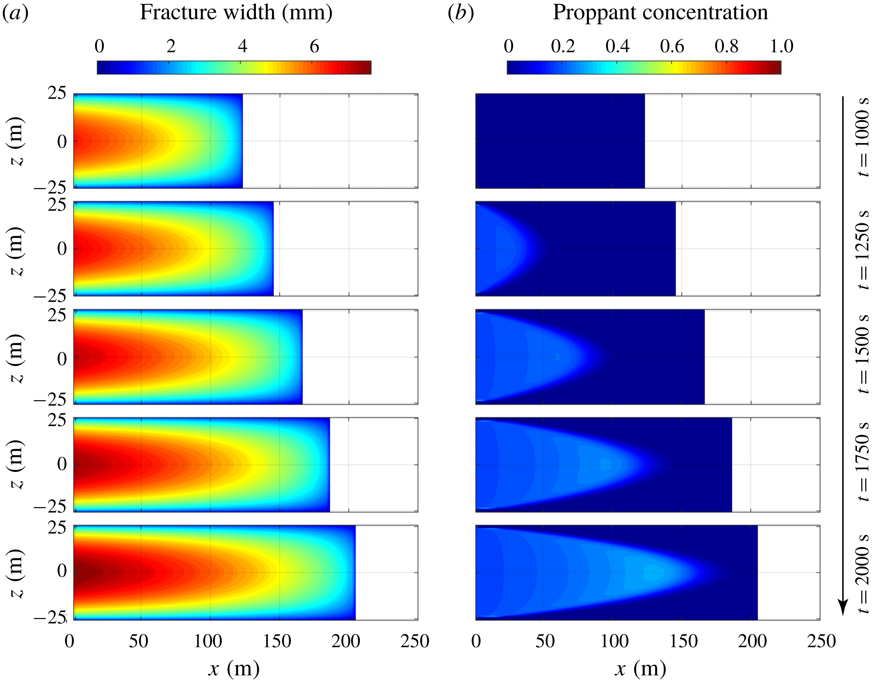
Figure 10 shows results for the case with an ultra-light-weight proppant (case 4). Ultra-light-weight proppants are developed to reduce proppant settling and are usually 25–60% lighter than commonly used sands, but are sufficiently strong to withstand reservoir stresses (Gu, Dao & Mohanty Reference Gu, Dao and Mohanty2015). In this case, the proppant density is set to be
 $1054~\text{kg}~\text{m}^{-3}$
. Similar to the case for the large proppant, the reduced proppant density has almost no influence on fracture propagation (figure 10
a). Since the proppant is only slightly denser than the fracturing fluid, gravitational settling is negligible and no apparent proppant bank is formed at the fracture base (as suggested by
 $S\approx 0.0075$
). As shown in figure 10(b), the proppant is distributed uniformly within the fracture at the conclusion of pumping.
Simulation results of the case with an ultra-light weight proppant (
 $\unicode[STIX]{x1D70C}_{p}=1054~\text{kg}~\text{m}^{-3}$
) at different snapshots in time
 $t=1000~\text{s}$
,
 $t=1250~\text{s}$
,
 $t=1500~\text{s}$
,
 $t=1750~\text{s}$
and
 $t=2000~\text{s}$
: (a) fracture geometry and (b) proppant distribution.

Simulation results of the case with large leak-off coefficient (
 $C_{l}=3.5\times 10^{-5}~\text{m}~\text{s}^{-1/2}$
) at different snapshots in time
 $t=1000~\text{s}$
,
 $t=1250~\text{s}$
,
 $t=1500~\text{s}$
,
 $t=1750~\text{s}$
and
 $t=2000~\text{s}$
: (a) fracture geometry and (b) proppant distribution.

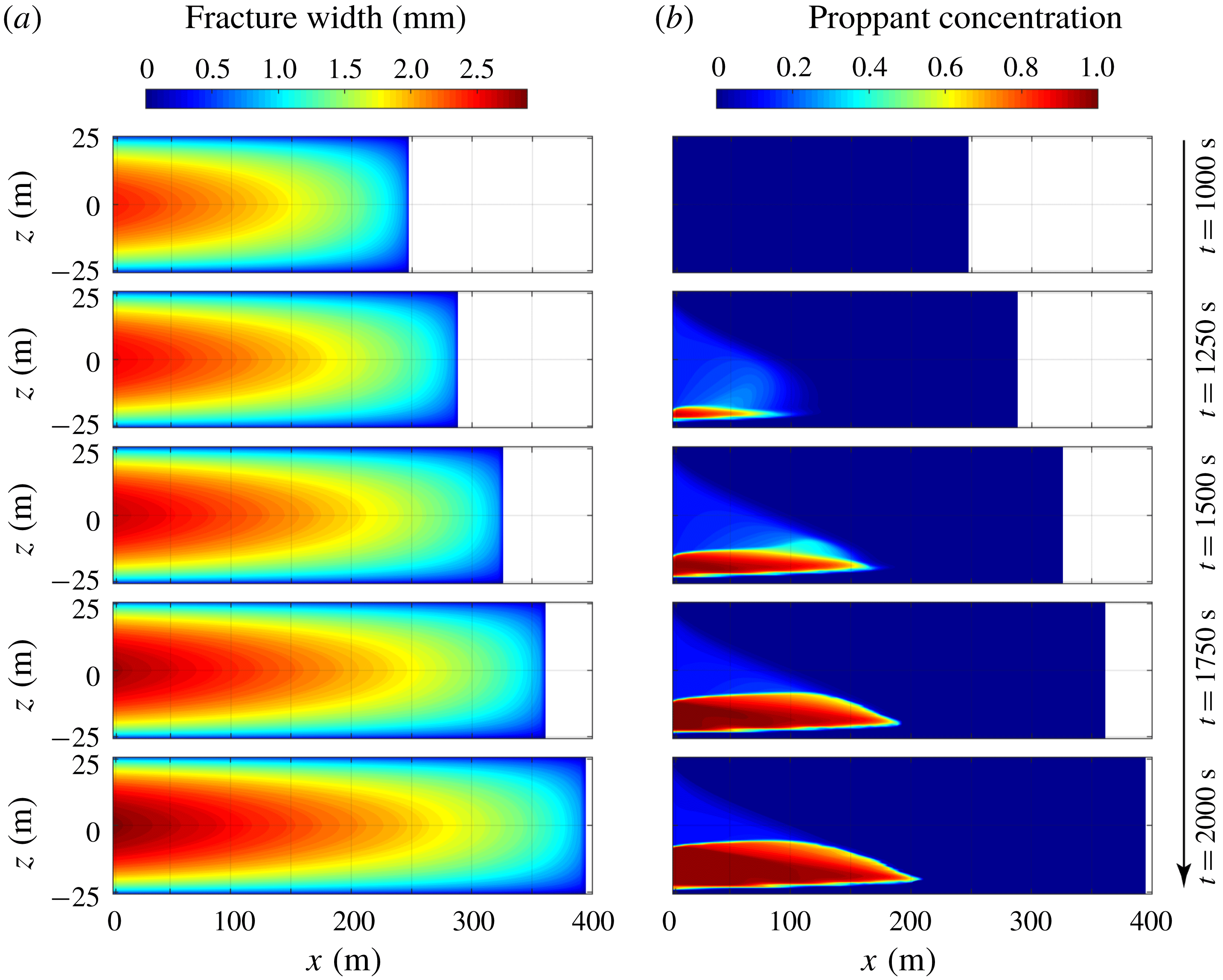
Simulation results of the case mimic slick-water fracturing (
 $\unicode[STIX]{x1D707}_{f}=0.001~\text{Pa}~\text{s}$
and
 $a=0.2~\text{mm}$
) at different snapshots in time
 $t=1000~\text{s}$
,
 $t=1250~\text{s}$
,
 $t=1500~\text{s}$
,
 $t=1750~\text{s}$
and
 $t=2000~\text{s}$
: (a) fracture geometry and (b) proppant distribution.

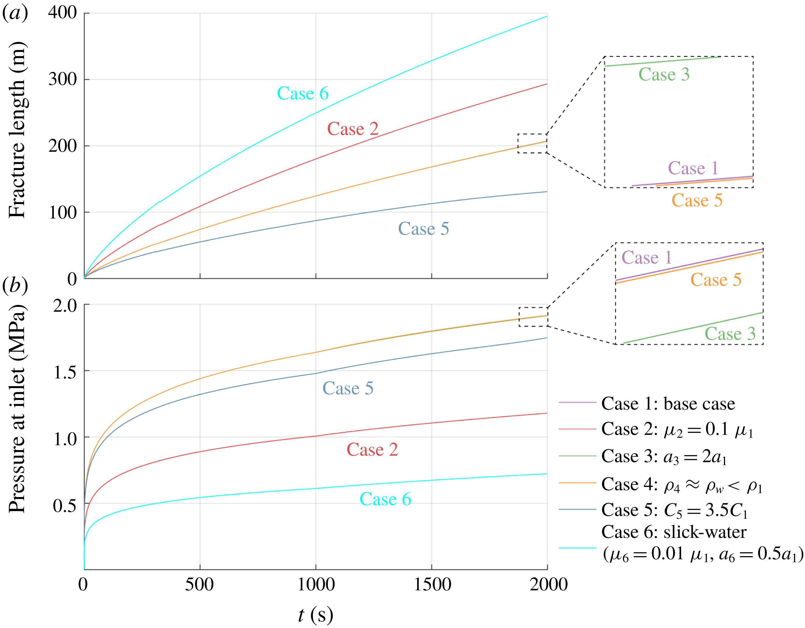
Evolution of (a) fracture length and (b) pressure at inlet with time for the six simulation cases.

Figure 11 shows the results for the case with increased leak-off (case 5), which might result from an increased permeability or effective-stress-dependent permeability of the surrounding formation (Wang et al.
Reference Wang, Elsworth and Denison2018a
). The Carter leak-off coefficient is set to
 $C_{l}=3.5\times 10^{-5}~\text{m}~\text{s}^{-1/2}$
– in this case 3.5 times larger than that used in the base case. As can be seen from figure 11(a), the resulting hydraulic fracture is
 ${\sim}128~\text{m}$
in length and as such considerably shorter than that corresponding to the base case. This is because a greater mass of fracturing fluid leaks off into formation instead of driving the propagation of the fracture. Under the same proppant injection schedule, the proppant rapidly reaches the fracture tip, resulting in premature tip screen-out. Thus, for hydraulic fracturing in a highly permeable formation, a higher injection rate or a longer pad injection duration is preferred to avoid this problem.
Figure 12 shows the simulation results for the case that mimics conventional slick-water fracturing (case 6). The viscosity of the fracturing fluid is assumed to be
 $\unicode[STIX]{x1D707}_{f}=0.001~\text{Pa}~\text{s}$
. Since a very narrow fracture is expected to result from such a low-viscosity fluid, the proppant is assumed to have a reduced size of
 $a=0.2~\text{mm}$
to ensure entry into the fracture. It can be seen from figure 12(a) that slick-water fracturing produces a long but very thin fracture – the fracture is
 ${\sim}395~\text{m}$
in length and has a maximum aperture of only
 ${\sim}2.9~\text{mm}$
when pumping stops. The extremely low viscosity of the fluid enables the proppant to rapidly settle to the fracture base, forming a proppant bank, although the smaller size of the proppant reduces settling velocity to some extent. Only a small portion of the fracture is propped at the conclusion of the pumping (figure 12
b). The value of
 $S$
is calculated to be
 ${\sim}5.23$
, which is much larger than the critical value of 1.0. Therefore, ultra-light-weight proppants might be beneficial in conventional slick-water fracturing to favour a more uniform distribution of the proppant. If the slick-water analysis is completed with a proppant density of
 $1054~\text{kg}~\text{m}^{-3}$
, the parameter
 $S$
will be reduced to only
 ${\sim}0.19$
, which is similar to that of the base case – confirming that proppant settling will be minor and that the proppant will be distributed relatively uniformly at the end of pumping.
Figures 13(a) and 13(b) show the fracture length and inlet pressure histories, respectively, for the various fracturing cases. It can be seen that, consistent with the discussions above, the case representing slick-water fracturing (case 6) produces the longest and narrowest fracture among the six simulation cases, while the case with fast leak-off rate (case 5) and the base case (case 1) show the shortest fracture length and largest inlet pressures, respectively. Elevated size and the reduced density of the proppant does not significantly influence fracture propagation, thus it is difficult to distinguish these two cases from the base case in the history curves (see the two zoomed-in windows in figure 13). Kinks in the evolution of inlet pressure with time are observed at
 $t=1000~\text{s}$
(figure 13
b), which corresponds to the beginning of proppant injection and results from the notable change in slurry viscosity.
4.3 Results of conductivity of closed hydraulic fractures
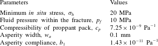
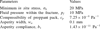
At the conclusion of pumping, fluid pressure decreases, enabling hydraulic fractures to close and compact the encased proppant packs. We perform simulations to define fracture closure for the six cases previously discussed (§ 4.1) for varied viscosities, particle sizes and densities, and leak-off rates. Residual fracture aperture, resulting fracture conductivity and stress applied on the proppant are analysed by assuming that the fluid pressure within the fracture is uniformly distributed. Any additional input parameters are listed in table 3, with all others consistent with those listed in table 2. Note that we assume both that the fracture stops propagating and that proppant transport ceases at the conclusion of pumping. However, formations with a low leak-off rate may delay full mechanical closure of the fracture and substantially extend this period of proppant advance and settling after shut-in, where proppant transport after shut-in might be considered to obtain a more accurate portrait of proppant distribution.
Input parameters for simulations of fracture closure.
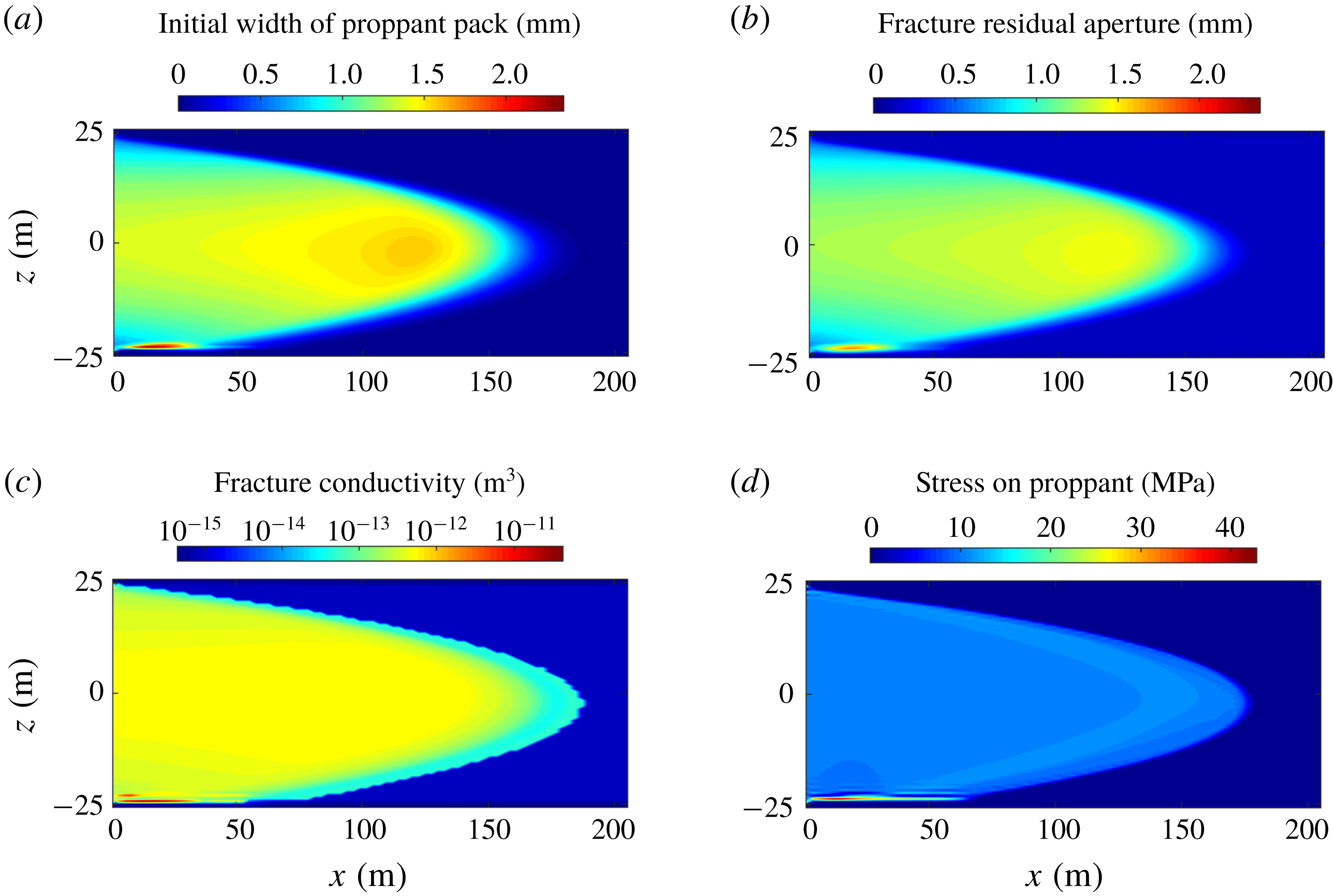
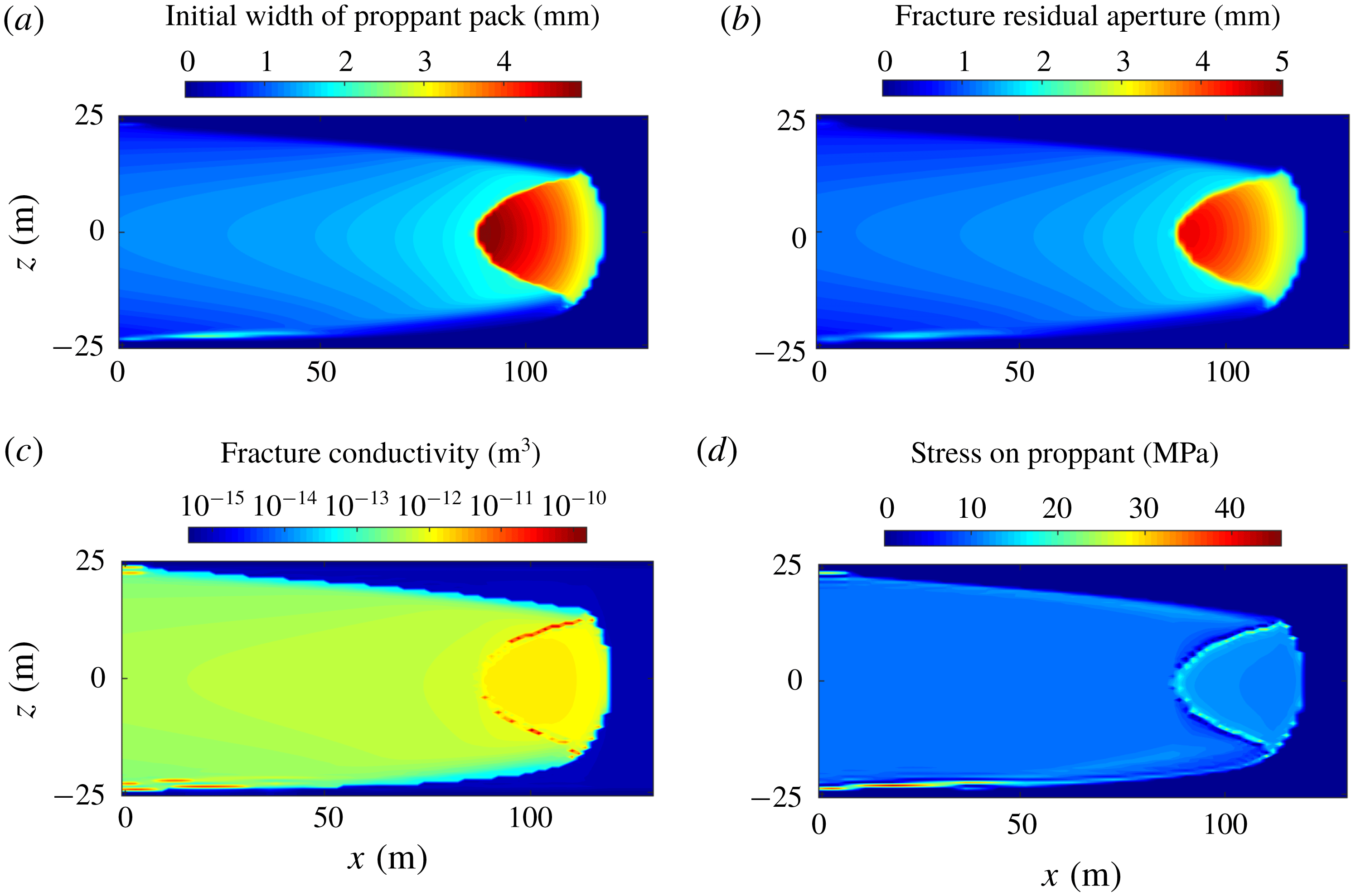
Simulation results of fracture closure for the base case: (a) initial width of proppant pack, (b) fracture residual aperture, (c) resulting fracture conductivity and (d) stress applied to the proppant pack.

Figure 14(a) shows the base case for the width of the proppant pack before compaction, i.e. when pumping stops, and figure 14(b–d) shows the fracture residual aperture, fracture conductivity and stress applied to the proppant, respectively, when the fluid pressure decreases to 10 MPa. As can be seen from figure 14(b), the propped portion of the fracture shows higher residual apertures which range from
 ${\sim}0.5~\text{mm}$
to
 ${\sim}1.75~\text{mm}$
and is
 ${\sim}0.5~\text{mm}$
smaller than the initial width of the proppant pack. The largest residual aperture is reached at the fracture base where a small proppant bank exists. The conductivity of the compacted proppant pack is distributed relatively uniformly and is of the order of
 $10^{-12}~\text{m}^{3}$
(figure 14
c). Two arching zones are formed around the proppant bank due to the flexural deformation of the fracture walls, as suggested by the extremely high conductivity (
 ${>}10^{-11}~\text{m}^{3}$
). For the unpropped portion, the fracture walls ultimately close onto facing asperities, resulting in small residual apertures. In the limit, this residual aperture is near null, and hence, compared to the propped portions of the fracture, an, extremely low conductivity, of the order of
 $10^{-15}~\text{m}^{3}$
, results. It is apparent from figure 14(d) that the proppant bank at the fracture base attracts a much higher stress than the proppant packs elsewhere. This indicates that the proppant particles within the bank may experience greater depths of embedment into the fracture walls and/or a larger potential for crushing and comminution.
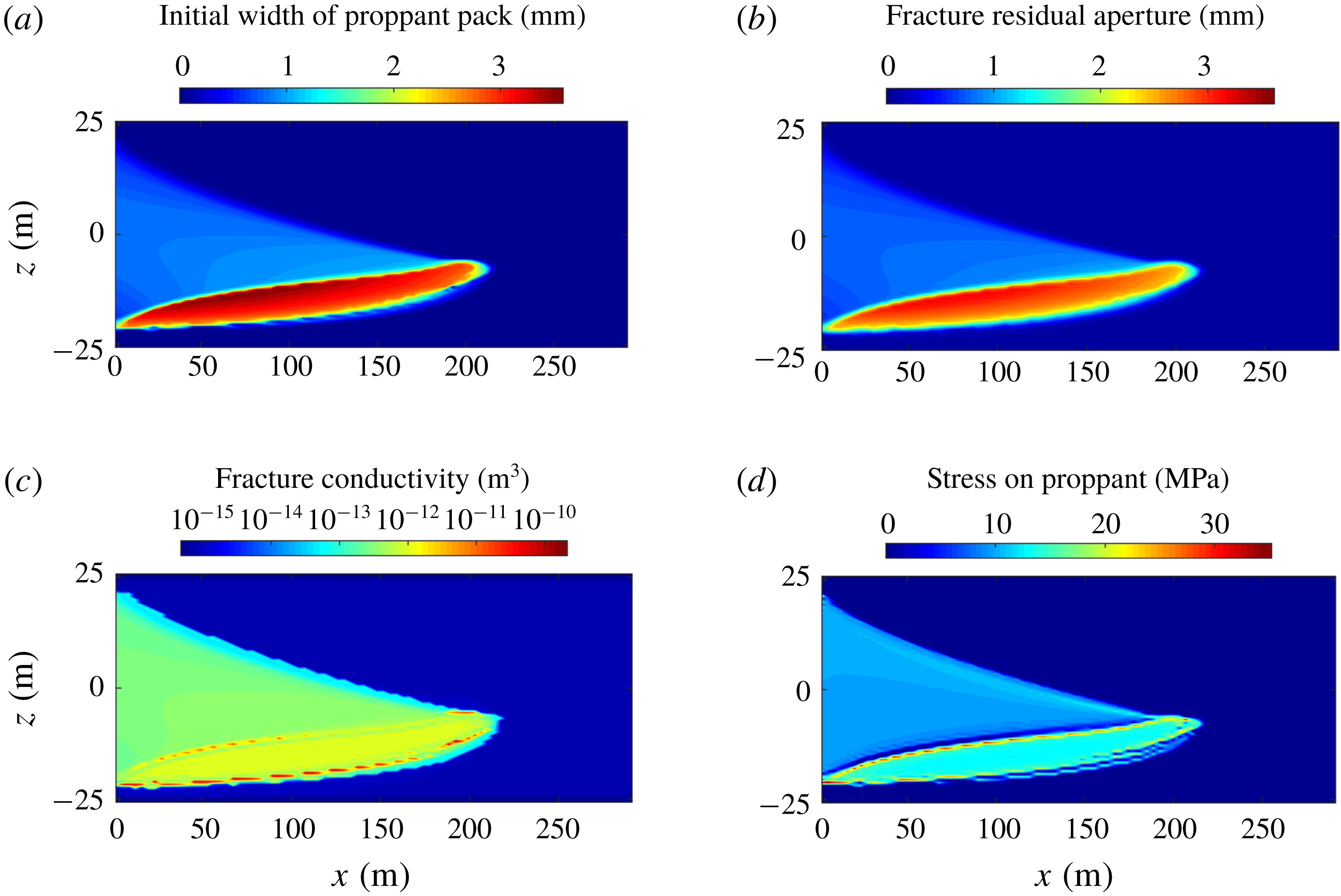
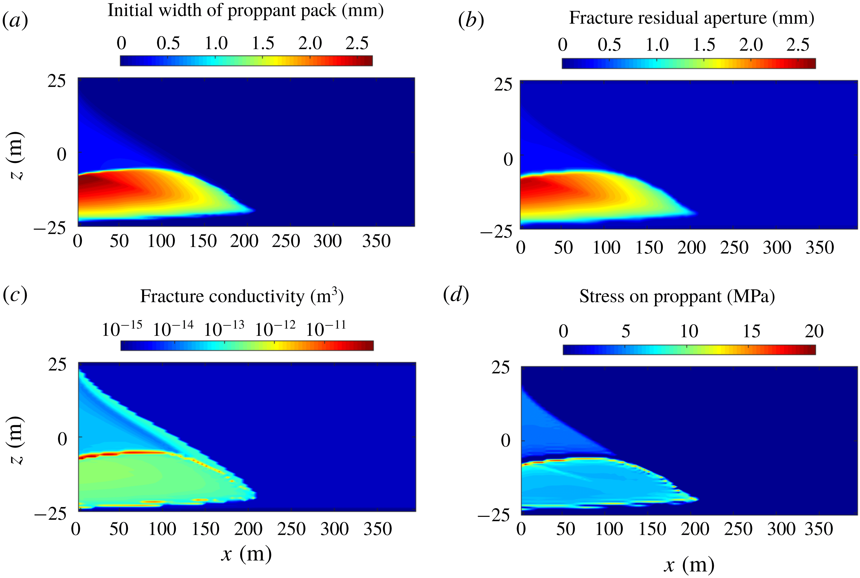
Simulation results of fracture closure for case with low fluid viscosity: (a) initial width of proppant pack, (b) fracture residual aperture, (c) resulting fracture conductivity and (d) stress applied to the proppant pack.

Figure 15 shows the results for fracture closure for the case with low fluid viscosity. Comparing figures 15(a) and 15(b), the proppant bank is compacted from a width of
 ${\sim}3.5$
to
 ${\sim}2.5~\text{mm}$
, with this compaction larger than that for proppant packs elsewhere due to the elevated compressive stress suggested by figure 15(d). Since the proppant particles are of the same size as those of the base case, the conductivities of the compacted proppant packs are similar (
 ${\sim}10^{-12}~\text{m}^{3}$
), although their residual apertures are slightly different. Two high-conductivity flow channels are observed in figure 15(c), present in the open and arched zones that form both above and below the proppant bank. The conductivity of those two channels is approximately two orders of magnitude larger than that of the proppant pack, and may significantly influence the distribution of fluid transport and improve overall fracture transmissivity. As can be seen from figure 15(d), these arch zones require higher stresses at top and bottom of the proppant bank, and leave the proppant particles next to the proppant bank uncompacted, as indicated by the zero stress applied on them – likely contributing to proppant flowback under sufficiently high flow rates.
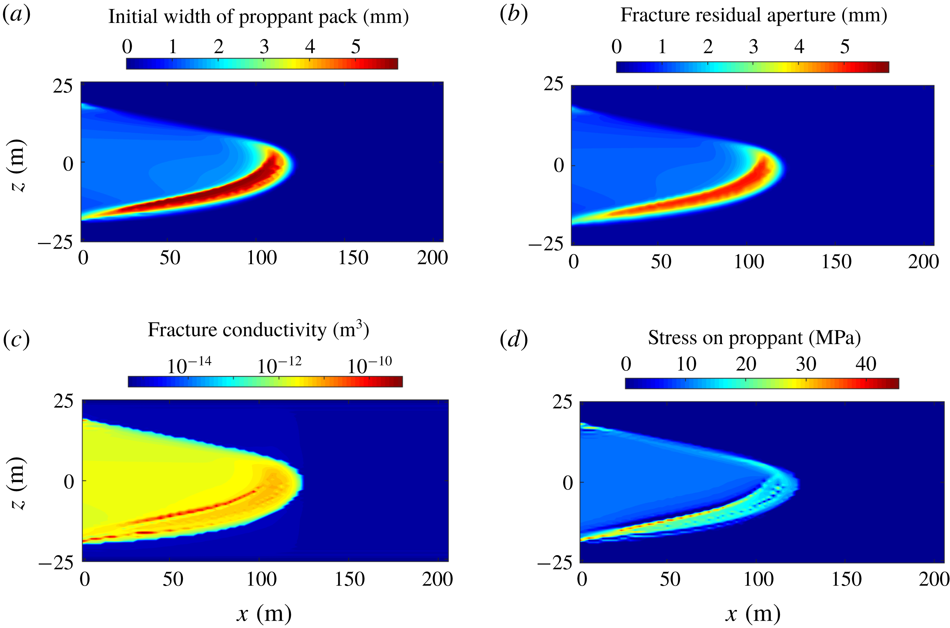
Simulation results of fracture closure for case with large proppant size: (a) initial width of proppant pack, (b) fracture residual aperture, (c) resulting fracture conductivity and (d) stress applied to the proppant pack.

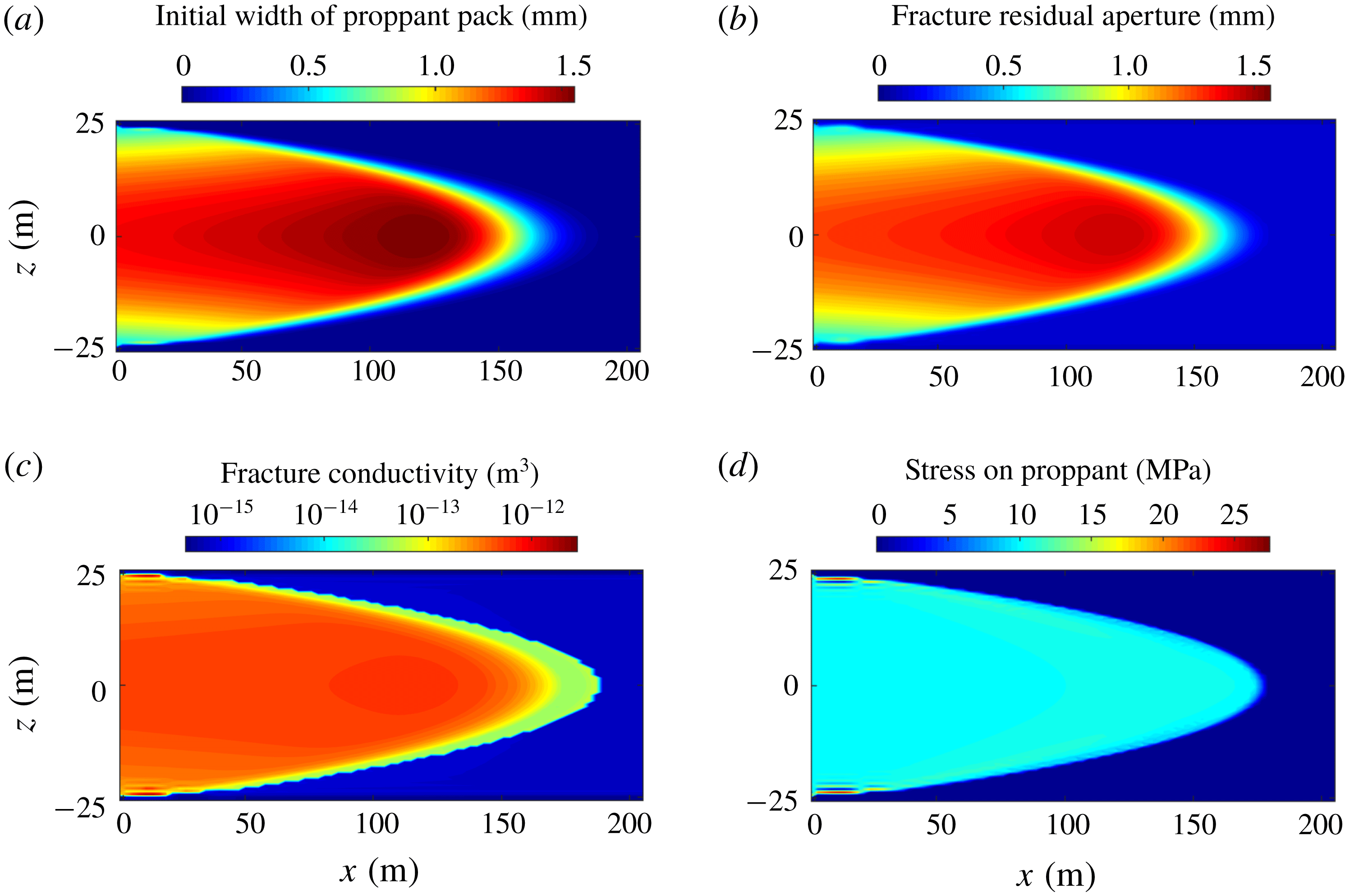
Simulation results of fracture closure for case with an ultra-light-weight proppant: (a) initial width of proppant pack, (b) fracture residual aperture, (c) resulting fracture conductivity and (d) stress applied to the proppant pack.

Simulation results of fracture closure for case with rapid leak-off: (a) initial width of proppant pack, (b) fracture residual aperture, (c) resulting fracture conductivity and (d) stress applied to the proppant pack.

Simulation results of fracture closure for case mimicking slick-water fracturing: (a) initial width of proppant pack, (b) fracture residual aperture, (c) resulting fracture conductivity and (d) stress applied to the proppant pack.

Figure 16 shows results for fracture closure for the case with large proppant size. As can be seen from figure 16(c), the propped portion of the fracture returns a conductivity approximately one order of magnitude larger than those in the above two cases. This is due to: (i) the fracture residual aperture being larger in this case (figure 16
b), and (ii) the influence of the intrinsically larger particle size in increasing the permeability of the proppant pack. The larger residual aperture also results in higher compactive stresses applied to the proppant bank, as shown in figure 16(d). The case with low proppant density exhibits almost the same behaviour in fracture closure as the base case, as can be seen from figure 17, except for the absence of influence from a small basal bank. For the case with a high leak-off rate, the proppant pack near the fracture tip, that results from tip screen-out, plays a similar role to that of a basal proppant bank – it absorbs the highest stresses, undergoes the greatest compaction (figures 18
a and 18
b) but supports surrounding high-conductivity channels that result from arching/bridging. However, a direct hydraulic connection between these arched open channels and the wellbore is absent – thus they may not be helpful to improve well performance. The results of fracture closure for the case mimicking slick-water fracturing are shown in figure 19. Although most proppant accumulates in a basal bank and achieves a high proppant concentration, the proppant pack remains very thin (figure 19
b), principally as a result of the thin fracture – thus the conductivity of the compacted bank is only of the order of
 ${\sim}10^{-13}~\text{m}^{3}$
(figure 19
c). Again, open flow paths develop adjacent to the proppant bank accompanied by high compactive stresses applied around its edge.
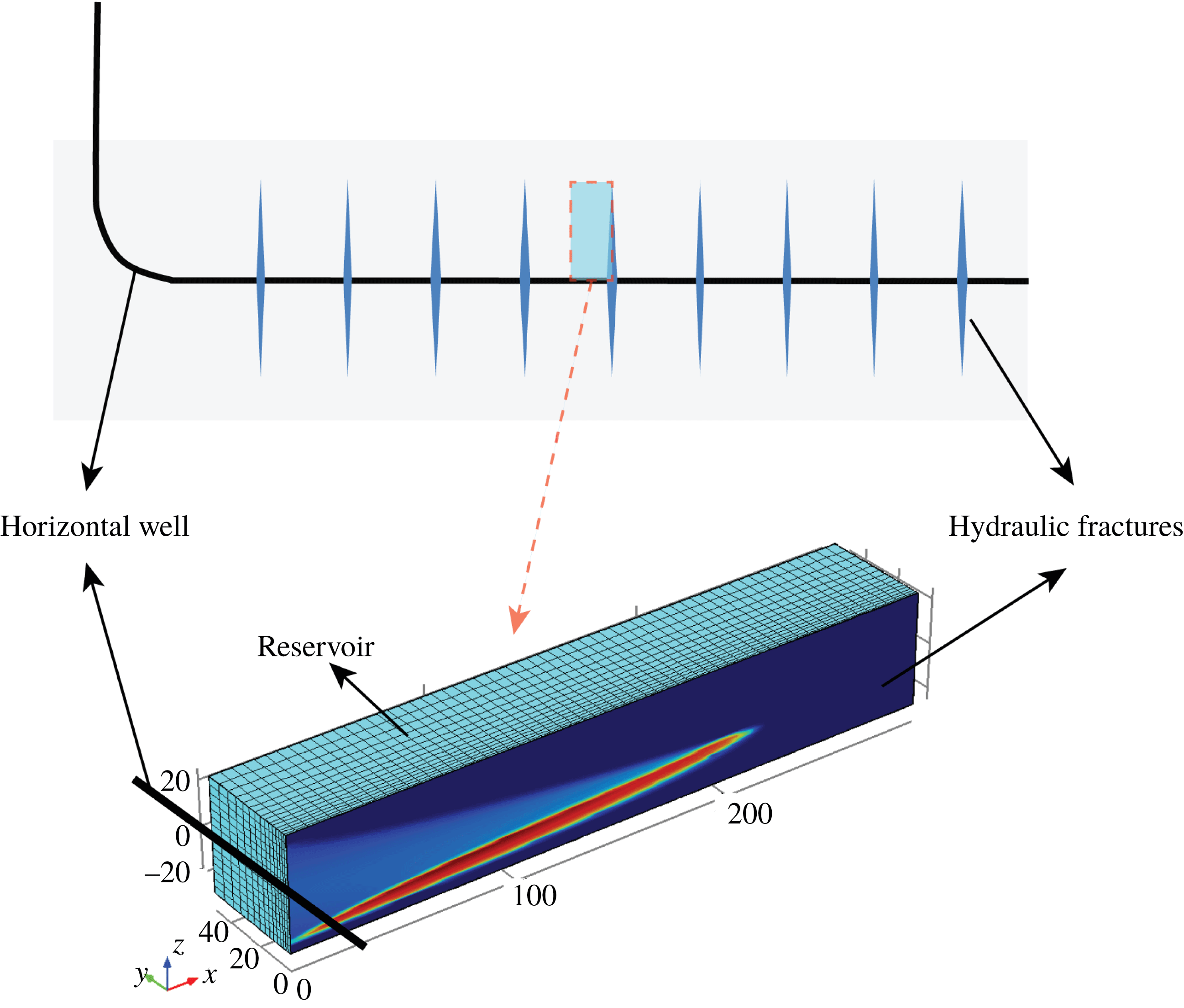
Schematic of the reservoir–fracture domain for the reservoir simulation model.

4.4 Results of reservoir simulations
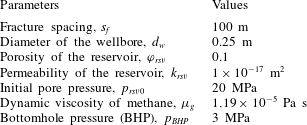
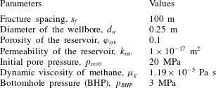
The fracture conductivities recovered from the fracture closure simulations (§ 4.2) are used in a reservoir simulation model to define the fluid flow paths that develop within hydraulic fractures and to predict the productivities of fractured wells. Figure 20 shows the reservoir–fracture domain for this reservoir simulation model. Taking advantage of the symmetry, only one wing of a fracture and half the matrix between the two adjacent fractures are simulated. The governing equations for gas flow within the reservoir and the fracture can be expressed, respectively, as
 $$\begin{eqnarray}\displaystyle \unicode[STIX]{x1D719}_{rsv}\unicode[STIX]{x1D70C}_{g}c_{g}\frac{\unicode[STIX]{x2202}p_{rsv}}{\unicode[STIX]{x2202}t}+\unicode[STIX]{x1D735}\boldsymbol{\cdot }\left(-\frac{k_{rsv}}{\unicode[STIX]{x1D707}_{g}}\unicode[STIX]{x1D70C}_{g}\unicode[STIX]{x1D735}p_{rsv}\right)=0, & & \displaystyle\end{eqnarray}$$
and
 $$\begin{eqnarray}\displaystyle w_{r}\unicode[STIX]{x1D711}_{r}\unicode[STIX]{x1D70C}_{g}c_{g}\frac{\unicode[STIX]{x2202}p_{f}}{\unicode[STIX]{x2202}t}+\unicode[STIX]{x1D735}\boldsymbol{\cdot }\left(-\frac{C_{f}}{\unicode[STIX]{x1D707}_{g}}\unicode[STIX]{x1D70C}_{g}\unicode[STIX]{x1D735}p_{f}\right)=\left.2\frac{k_{rsv}}{\unicode[STIX]{x1D707}_{g}}\unicode[STIX]{x1D735}p_{rsv}\right|_{y=0}, & & \displaystyle\end{eqnarray}$$
where
 $p_{rsv}$
and
 $p_{f}$
are two unknown pressures in the reservoir and fracture, respectively;
 $\unicode[STIX]{x1D719}_{rsv}$
and
 $k_{rsv}$
respectively represent porosity and permeability of the reservoir;
 $\unicode[STIX]{x1D70C}_{g}$
and
 $c_{g}$
are density and compressibility of methane, respectively, and are functions of fluid pressure which can be obtained from the NIST database (Lemmon Reference Lemmon1998);
 $\unicode[STIX]{x1D707}_{g}$
is the dynamic viscosity of methane;
 $w_{r}$
,
 $\unicode[STIX]{x1D711}_{r}$
and
 $C_{f}$
represent fracture residual aperture, porosity of the compacted proppant pack, and fracture conductivity, respectively, and these are obtained from the simulation results (§ 4.2). Equation (4.3) is defined in the whole three-dimensional domain, as shown in figure 20, while (4.4) is defined only in the hydraulic fracture, i.e. in the plane
 $y=0$
. Boundary conditions for (4.3) are that
 $\left.p_{rsv}(x,z)\right|_{y=0}=p_{f}(x,z)$
and the other boundaries are set as no flow. For (4.4), all the boundaries are set as no flow, except that a production well is located at the origin. A constant bottomhole pressure (BHP) is assumed throughout the production lifetime. Initially, pore pressures within both the reservoir and the fracture are set to be a constant. This reservoir simulation model, i.e. (4.3) and (4.4) together with boundary and initial conditions, is solved using COMSOL Multiphysics (FEM-based) with input parameters listed in table 4.
Input parameters for the reservoir simulation.
Fluid flow paths in the hydraulic fractures at
 $t=1~\text{year}$
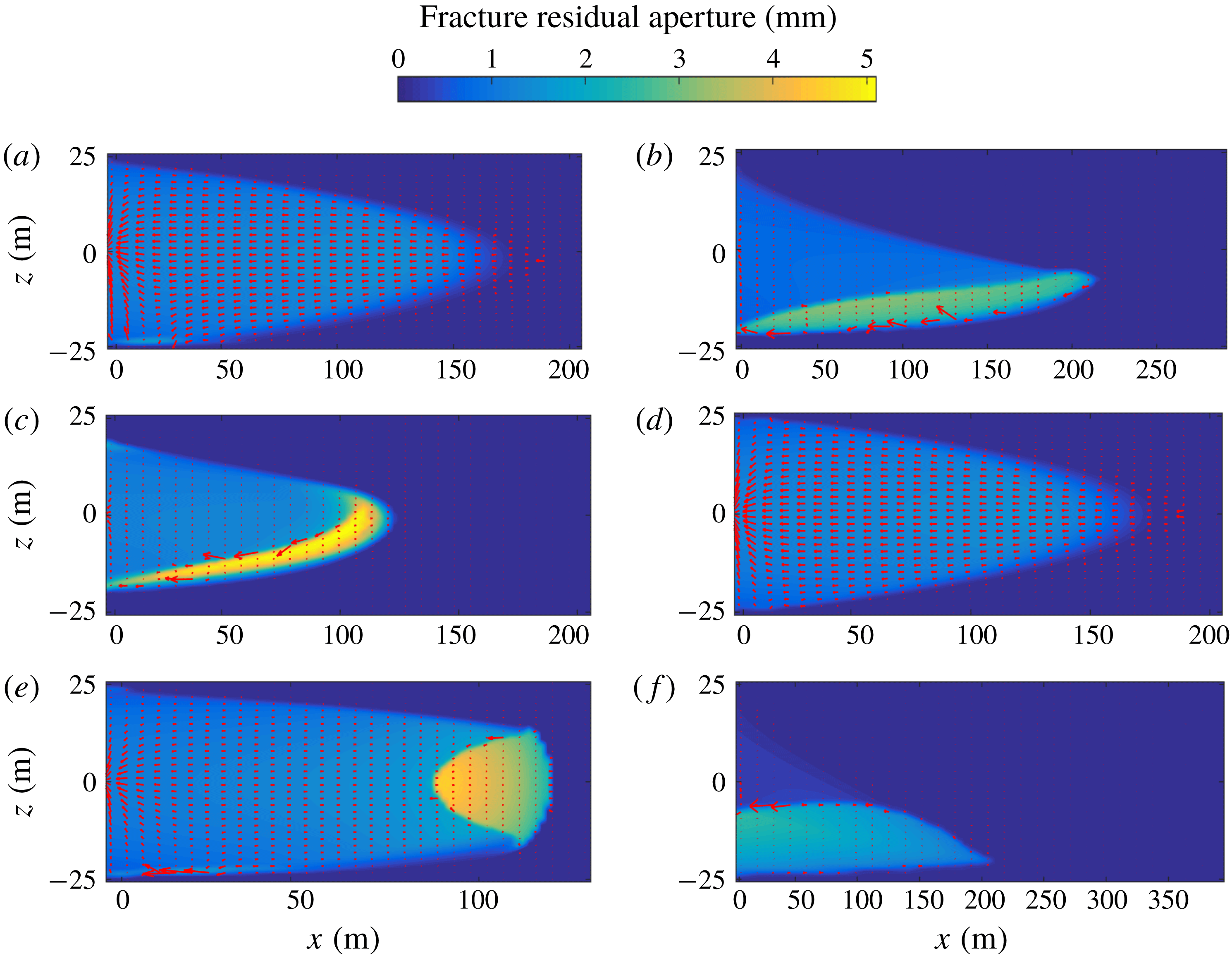
for (a) the base case, and cases with (b) low fluid viscosity, (c) large proppant size, (d) ultra-light-weight proppant, (e) rapid leak-off rates and (f) slick-water fracturing. The red arrows show the flow velocity fields, and the backgrounds show the fracture residual apertures for the six cases to a uniform scale.

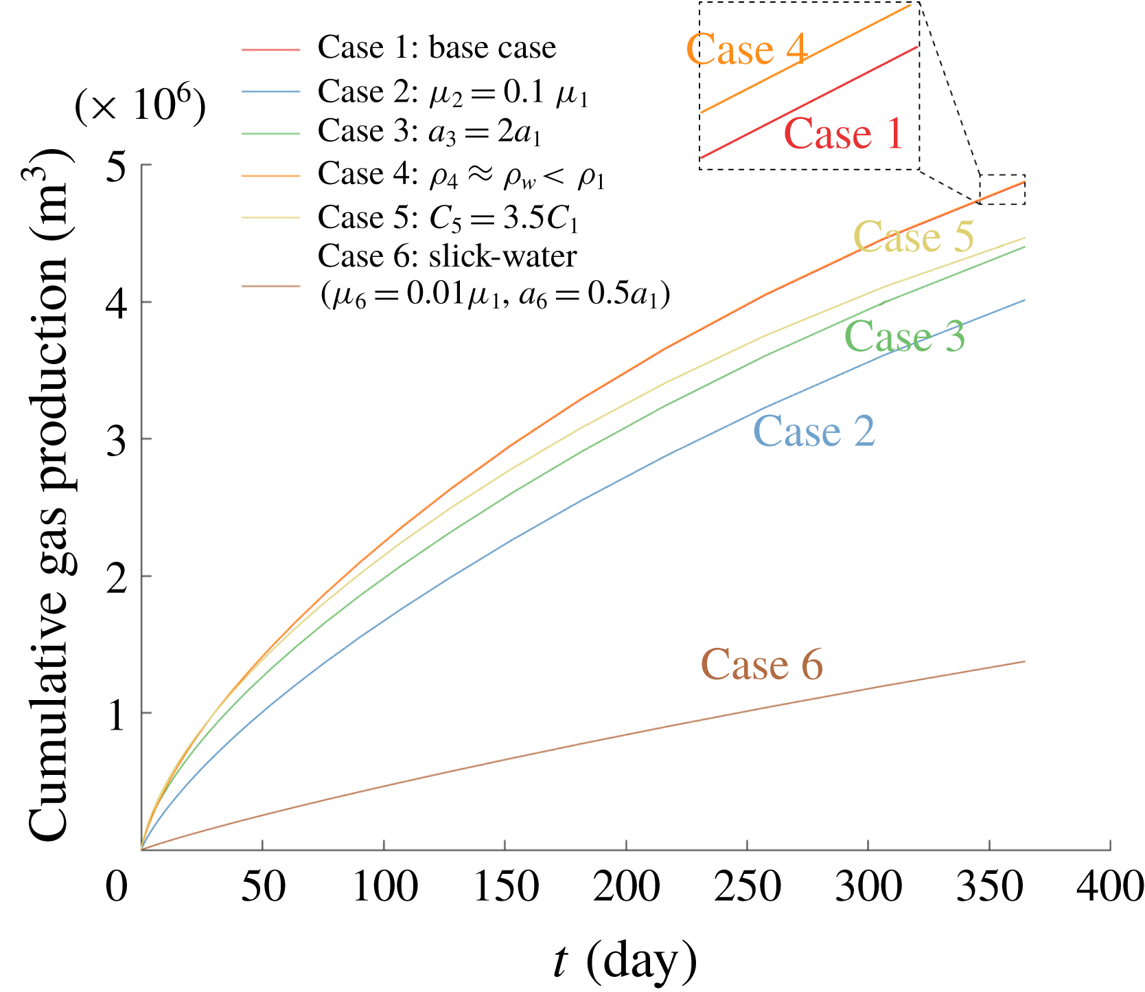
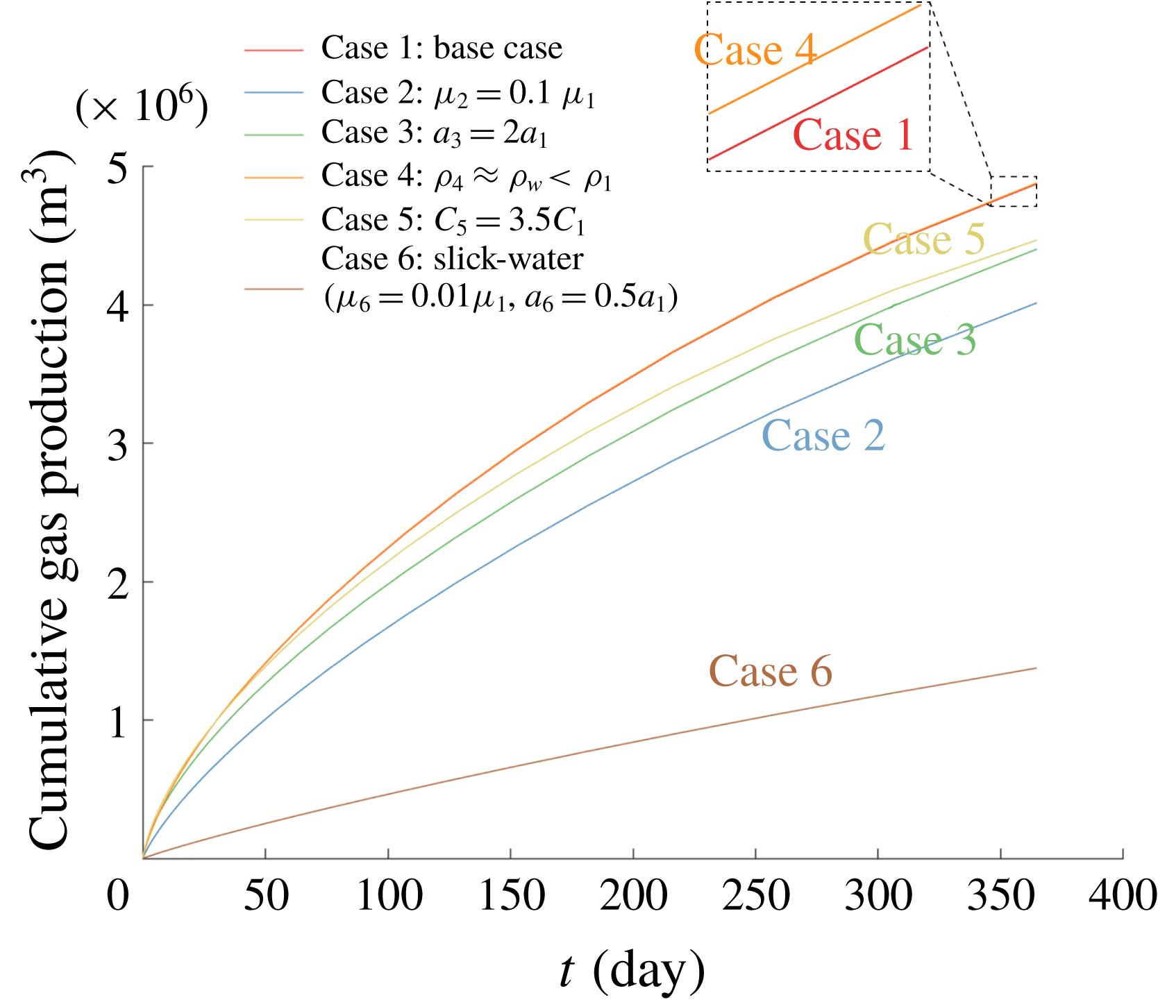
Figure 21 shows the fluid flow paths in the hydraulic fractures when production has extended over one year for the six cases previously described (§ 4.2). The red arrows identify the velocity field of the fluid flow, and the background colour indicates the fracture residual apertures for the six cases to a uniform scale. As discussed earlier, relatively uniform proppant distributions are obtained for the base case and the cases with ultra-light-weight proppant and rapid leak-off. As a result, the hydrocarbon, which diffuses from the matrix into the hydraulic fractures, flows towards the production wells homogeneously through the proppant packs, as shown in figures 21(a), 21(d) and 21(e). For the cases with low fluid viscosity, large proppant size and for slick-water fracturing (low viscosity and small proppant), basal proppant banks develop and complex conductivity distributions after fracture closure has occurred. This in turn significantly influences the distribution of fluid transport during production. As can be seen from figures 21(b), 21(c) and 21(f), the high-conductivity arch zones formed around the proppant banks offer preferential flow channels for hydrocarbon recovery. This effect may play an important role for the accurate prediction of production mechanisms and mass rates; however, it is ignored in much of the contemporary literature (e.g. Gu & Mohanty (Reference Gu and Mohanty2014), Yu et al. (Reference Yu, Zhang, Du and Sepehrnoori2015) and Shiozawa & McClure (Reference Shiozawa and McClure2016)). Figure 22 shows cumulative gas production with time for the six simulations. It can be seen that the production of the case with ultra-light-weight proppant is the highest and that of the base case is only slightly lower. The case with rapid leak-off also exhibits higher production than the other three cases where a basal proppant bank is observed, although its fracture is much shorter. This results from the fact that only a small portion of the fracture is propped open in the cases with a basal bank (i.e. cases with low fluid viscosity, large proppant size and slick-water fracturing). Even though the high-conductivity flow channels do provide benefits in improving gas production rates, they are vertically unconnected to the top of the pay zone, resulting in a longer diffusion distance for the hydrocarbon in that region. The case with slick-water fracturing shows the lowest production, despite it having created the longest fracture. This is because the thin proppant packs exhibits limited conductivity which then contributes only modestly to production.
Cumulative gas production versus time of the six simulations.
5 Conclusions
A numerical model is developed to describe the propagation of a blade-shaped fluid-driven fracture, concurrent with proppant transport, and followed by fracture deflation at the conclusion of pumping. This formalism is used to define the evolution of fracture conductivity, first with the advection of proppant into the inflated and propagating fracture, and then as a result of fracture and proppant pack compaction as hydraulic pressure decreases after the cessation of pumping. Fracture propagation is established based on the PKN-formalism. Proppant transport is represented as a slurry (fluid–solid mixture) with proppant distribution defined through its volumetric concentration. An empirical constitutive law for the slurry (Dontsov & Peirce Reference Dontsov and Peirce2014) is employed to describe its rheology, its transition from Poiseuille flow to Darcy filtration flow, proppant motion with fluid flow and gravitational settling of the proppant. A blocking function is introduced to incorporate the effect of proppant screen-out. The approach introduced by Wang & Elsworth (Reference Wang and Elsworth2018) is used to follow the evolution of fluid conductivity in the closed fracture. This model is capable of accommodating the mechanical response of proppant packs, fracture closure between rough fractures in contact, proppant embedment into fracture walls, and flexural displacement of the unsupported spans of the fracture. Reservoir simulations are performed to explore the evolution of heterogeneous fluid flow paths within the hydraulic fracture during production, and ultimately to predict hydrocarbon production rates.
Parametric studies are completed to explore the effects of fluid viscosity, proppant size, proppant density and leak-off rate on the resulting fracture geometry and proppant distribution. Results show that reduced fluid viscosity increases fracture length but narrows down fracture width, and accelerates proppant settling from suspension accumulating into a basal bank. Proppant size and density do not significantly influence the length of fracture propagation. Relative to the reference case, larger proppant settles faster and bridges earlier even when it is distant from the fracture tip, limiting its penetration from the wellbore into the accessed reservoir. Ultra-light-weight proppants exhibit negligible settling and as a result may be distributed relatively uniformly along the fracture at the conclusion of pumping. Rapid leak-off into the formation may prematurely arrest fracture propagation, leaving the fractures both shorter and narrower and with premature tip screen-out relative to the case without excessive leak-off. The commonly used slick-water fracturing tends to create long but very narrow fractures and requires small diameter proppant to ensure its entrance into the fracture. However, proppant settling is severe due to the extremely low viscosity of the slick water, even though a small proppant size hinders settling, to some extent.
At the conclusion of pumping, the monotonic decrease in fluid pressure allows the fracture to deflate and compact the proppant pack. Proppant packs show higher conductivity than the unpropped, closed portion of fractures. The conductivity of the proppant pack is further enhanced by larger proppant size. High-conductivity flow channels form around proppant banks due to the flexural displacement of the fracture walls, where spans arch across an empty or low concentration proppant pack void. These channels necessarily prompt high compactive stress rims around the edge of the proppant banks, where the proppant particles may experience greater depths of embedment into the fracture walls and/or a larger potential for crushing and comminution. Reservoir simulations show that these open channels provide preferential flow pathways for the hydrocarbon recovery and enhance fracture efficiency and well performance. Fractures with more effective vertical proppant placement achieve higher cumulative gas production, while those encasing a proppant bank exhibit a reduced production rate due to the limited propped area of the fractures. Although relatively comprehensive, the current model is unable to accommodate fracture propagation and proppant transport after shut-in. This is not viewed as an important limitation, but this effect may be significant if leak-off rate is sufficiently slow.
Acknowledgements
This work is the result of support from DOE under the Small Business Innovative Research (SBIR) programme (grant number: DE-SC0013217). This support is gratefully acknowledged.