

1. Introduction
There's nothing like a good statistics textbook to put a person to sleep. I say this as a way of acknowledging that my topic of statistics is not one that makes many people's heart race. However, since there are reports that up to 86% of empirical research articles in leading second language acquisition (SLA) journals are quantitative (Gass Reference Gass, Bhatia and Ritchie2009) and probably contain some statistical analysis, I think it's of the utmost importance that we use the best statistics possible. That's why my talk today will introduce something called robust statistics. Robust statistics include a variety of techniques developed by statisticians that are much better at accommodating real data than either classic parametric techniques or non-parametric techniques. I hope I am not being too offensive when I draw an analogy here about ignoring modern developments in neighboring fields, but resistance to new ways of doing statistics makes me think of what happens sometimes in fields peripheral to SLA, where students have been taught that second language acquisition essentially consists of Krashen's Monitor Model (Reference Krashen, Burt, Dulay and Finocchairo1977). Rand Wilcox, a psychologist who is trying to introduce robust statistics into his field, claims that many discoveries are being lost by ignoring modern statistical methods (Wilcox Reference Wilcox1998).
I think the first obstacle to convincing people to change their statistical ways lies in their incomplete understanding of statistics, especially in our statistical intuitions. The following scenario was laid out by two psychologists addressing other researchers at an academic conference (Tversky & Kahneman Reference Tversky and Kahneman1971: 107):
Suppose you have run an experiment on 20 subjects, and have obtained a significant result which confirms your theory (z = 2.23, p < .05, two-tailed). You now have cause to run an additional group of 10 subjects. What do you think the probability is that the results will be statistical, by a one-tailed test, separately for this group?
Let me make this question easier – do you think the probability of finding a statistically significant result for the additional group is 95%, 85%, 75%, or 50%?Footnote 1 Let's look at another, similar question from Tversky & Kahneman (Reference Tversky and Kahneman1971: 107):
Suppose one of your doctoral students has completed a difficult and time-consuming experiment on 40 animals. He has scored and analyzed a large number of variables. His results are generally inconclusive, but one before-after comparison yields a highly significant t = 2.70, which is surprising and could be of major theoretical significance. Considering the importance of the result, its surprisal value, and the number of analyses that your student has performed – would you recommend that he replicate the study before publishing? If you recommend replication, how many animals would you urge him to run?
Most of the psychologists that the authors casually surveyed at their conference (66 out of 75) recommended replication with 20 more subjects. Since the authors anticipated this result, they added an additional question (Tversky & Kahneman Reference Tversky and Kahneman1971: 107–108):
Assume that your unhappy student has in fact repeated the initial study with 20 additional animals, and has obtained an insignificant result in the same direction, t = 1.24. What would you recommend now? Check one:
(a) He should pool the results and publish his conclusion as fact.
(b) He should report the results as a tentative finding.
(c) He should run another group of [median –20] animals.
(d) He should try to find an explanation for the difference between the two groups.
Which is your answer? Tversky & Kahneman (Reference Tversky and Kahneman1971) say that most people's intuition is that the replication was a failure. However, the authors point out that given the original findings, this replication result with only half the number of subjects (just 20 the second time) is about as successful as it could possibly be, and points to a real and statistically supported finding. Unless you correctly guessed 50% for the first scenario and chose answer (a) for the second scenario, your intuition matches those of most of the psychologists that Tversky & Kahneman surveyed, which is that a replication, no matter the size, should match the findings of the first experiment.
The problem with intuition here is that we expect samples to be highly representative of the population. In other words, if there really is an effect in the population, we expect that no matter the size of the sample, it should reflect the true nature of the population: it should show up whether 10, 20, or 40 subjects are tested. However, p-values are highly dependent on sample size, so that in the first example given above, the probability of obtaining a statistically significant result (where the p-value is below .05) with half the original number of participants is only about 50%. A similar result will hold for a replication of the second example, meaning that the dissertation advisor directed their student to invest much energy and time on a project that even at its best would have only a 50% chance of being successful!
Tversky & Kahneman (Reference Tversky and Kahneman1971) note that this belief in the representativeness of samples, no matter their size, leads to something called the ‘gambler's fallacy’. For example, most people know that the odds of getting heads when flipping a coin is 50%, so if there has been a long run of tails they may think that the odds of getting a head soon are increased because there needs to be a correction. In other words, lay people expect a random process to be self-correcting. However, the odds are 50% only in the long run, with a large number of samples. In the short run it is not at all uncommon to find long runs of the same result (and the odds of getting heads never increase to more than 50% for any single flip!).
Thus note that both of these mistaken statistical intuitions – that samples are representative of the population no matter their size, and that random processes are self-correcting – lead real people to make real statistical decisions that may be completely erroneous. One of the most damaging for a field of inquiry may be represented by choice (d) in the example of the dissertation student. When faced with a result that is not statistically significant (and one hoped it would be), theoretical explanations for that result may be put forth and shape the course of future research. However, the actual reality may be – and in this case it is – that the results were due to the numbers of subjects tested. Those recommending replication in the dissertation student example may have done so because they suspected the first result happened by chance because of the large number of tests performed. When the results of the replication found the same trend (that there was something going on with that one variable), albeit not a statistically significant one because of the smaller number of subjects, it too was discounted! If the dissertation advisor in the second example had understood statistics and the law of large numbers better, they would have recommended publication of the results or at least replication with 20 more subjects!
The upshot of this discussion is to show that our naive intuition will lead us astray when it comes to the variability we expect in samples. We will expect less variability in samples than we should. We will assume that small samples are just as representative as large samples. We will tend to discount statistically non-significant results whose p-values are above .05 without considering that the p-value is high because of a small sample size, and that the results may actually indicate something important (which we can ascertain through effect sizes).
The problem that I want to address in this paper is precisely the problem mentioned here: the assumption that difficulties in finding statistical results can be attributed to the nature of the data or the research methodology, when researchers should in fact be looking first to their statistics for the source of problems.
2. Classical statistics and assumptions
Classical statistics, the kind of parametric statistics that most readers of this article will be used to seeing (such as ANOVA, correlation, or t-tests) came into use at least early in the twentieth century, if not before in some cases. In order to simplify the calculations necessary to determine the probability of the statistics (such as F for the ANOVA test or r for correlation) if the null hypothesis is true, statisticians devised tests that assumed a normal distribution of data. Since the normal distribution has some clearly defined properties, making this assumption meant that probability tables could be calculated once, and statistical users could then consult those tables to look up the probability of the statistic (the p-value).
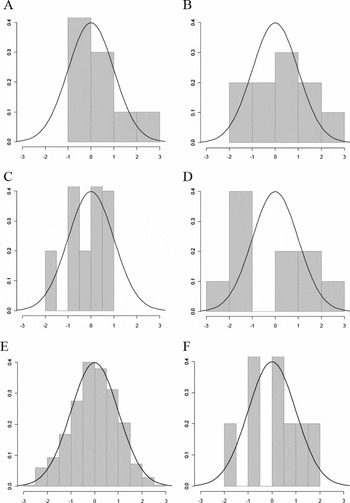
This approach was probably the best choice for the time, given the difficulty in doing complex mathematical calculations without computers, but it also results in a problem if the data are not exactly normally distributed. In other words, what I'm saying is that the assumptions of parametric statistics are exact, not approximate (Huber Reference Huber1981; Maronna, Martin & Yohai Reference Maronna, Martin and Yohai2006). This was something I didn't know before. Close is good enough for horseshoes and hand grenades, but even small departures from normality can sometimes have a large effect on statistical conclusions. However, with small sample sizes (less than 50 in a groupFootnote 2, which may still be too small), it is basically impossible to tell whether data really are normally distributed or not. An example may illustrate the point well. Look at Figure 1 and decide which distributions are non-normal. The histograms in Figure 1 are all overlaid with a normal density curve to help you with this task. You can find the R code I used to generate this figure on the Language Teaching website, http://journals.cambridge.org/lta, as Appendix A (R development core team 2009).
Six histograms showing the density of the distribution

You may well have said that every histogram except for E was non-normal. Only the figure in 1E had the nice bunching of data in the middle and the smooth reduction of data in the tails that most people associate with the ‘bell curve’ of a normal distribution. However, every single one of the histograms was sampled from a normal distribution! All the histograms except for E were sampled with only ten data points, while E contained 500. The point I am trying to make with this figure is that your sample may well be from a normal distribution, but with only ten (or 15 or 20) participants in a group, you basically cannot tell whether the population distribution is normal or not. This reminds us of what I mentioned at the beginning of the paper – we cannot expect small samples to reflect the properties of the population in the same way as large samples.
The question we must then ask ourselves is, well, should we assume that our data are from a normal distribution or not? Since very few researchers have even 50 participants in a group, it seems basically impossible to tell whether our data are normally distributed, so should we just go on and assume that our data are normally distributed and use parametric statistics? What is the alternative? Non-parametric statistics are also available, and most people know that non-parametric statistics do not require a normal distribution of data (although they do have other requirements).
However, there are problems both with using parametric statistics if your data are not normally distributed, and with using non-parametric statistics if your data are normally distributed. Both these paths, however, will result in less power, so I'd like to discuss the concept of power in a little more detail. Power is a number that represents the probability of detecting a statistical result when there are true differences between groups or true relationships between variables. Power, then, is the ability to find out the truth in a statistical situationFootnote 3. If power is .80, this means that you have a 20% chance of concluding that there is no difference between groups or no relationship between variables when in fact there is one. In other words, even if your power is high (and most statisticians would say power = .80 is a high or desirable level), all of your effort and time and expense to find out what is going on in your experiment may, in 20% of the cases, be rendered ineffective.
Consider, on the other hand, how much importance we give to avoiding the opposite problem, that of concluding that there is a difference between groups or a relationship between variables, when in fact there is not (also called a Type I error). If you set your alpha level to .05 then the probability of this problem is very low, at 5%. So there is an imbalance between our opposite problems. On the one hand, we set our probability of being overeager to find differences very low (at only 5%); on the other hand, we set our probability of being too cautious much higher even in the best-case scenario (at 20% if power is good, and higher if our power is lower). In fact, we can expect that the probability of being overly cautious (the Type II error, or numerically the number ‘1’ minus the level of power) is quite high in most studies. For my SPSS book (Larson-Hall Reference Larson-Hall2010) I analyzed the power in several of my published studies and found that in one case I had 63% power, in another 27% power, and in another 57% power. This is not very high – I guess I was lucky to find some results!
If we want to balance the probabilities of the two problems more evenly, we ought to be concentrating more on increasing power than we do. Let me repeat that, because it is really the crux of what I'm trying to get at in this paper: we need to be more concerned with increasing our power than increasing our conservatism. We are already guarding well against being overeager to find results, but in most cases we are not doing a good job balancing that concern against the concern to find real results (having the power to do that).
The most difficult way to increase power, but one that is clearly important, is to increase sample size. However, there are two other ways to increase power that do not require as much work. One way is to raise the accepted alpha level to .10, meaning that any p-value under .10 is considered statistically significant. An increase in the acceptable type I error rate will increase power to find differences. Another way to increase power, and what I am arguing for in this paper, is to use more powerful statistics. And in most cases, robust statistics are more powerful than both parametric and non-parametric statistics (Wilcox Reference Wilcox2005).
3. Power and conservatism
Given some of the comments I've received after a talk on this subject, I get the sense that researchers in the field are uncomfortable with the idea of using robust statistics, because they feel that increasing the power of statistics is somehow cheating. Cheating means, of course, going against the rules of whatever game we are playing, and statistics may sometimes seem like a game with arbitrary conventions.
For example, there are published studies which report a p-value very close to, but a little larger than, .05. In this case, the author does not claim that the result was statistically significant, although if they were hoping to find differences between groups or relationships between variables they may note that the p-value is close to .05. In other cases with the same p-value, the author may report that there is no difference between groups or no relationship between variables. For example, Abrahamsson & Hyltenstam (Reference Abrahamsson and Hyltenstam2008) report that there is a correlation between aptitude and grammaticality judgment tests (GJT) scores for early learners of L2 Swedish (r = .70, p < .001), but no correlation between aptitude and GJT scores for native speaker controls (r = .47, p = .077). The authors claim that ‘for the native speakers, aptitude and grammatical intuition seem to be unrelated’ (Reference Abrahamsson and Hyltenstam2008: 497). If we changed the acceptable alpha rate to .10 instead of the usual .05, then the authors would be forced to conclude that there was indeed a correlation between aptitude and GJT scores for the native speakers as well (note how increasing the alpha level gives us more power to find differences). Would it thus be cheating to change the entire course of argumentation about which groups have significant (and by this I mean important) interactions between aptitude and grammatical intuition?
My answer is no. In fact, in this case the problem with the whole false dichotomy between ‘statistically significant’ and ‘statistically non-significant’ at the α = 0.5 mark becomes quite clear with an example such as this. Since the effect size for correlations is evident in the r-value that is reported, we can see that the correlation between aptitude and grammatical intuition explains more of the variance for the early learners (R2 = .49, or 49%) than for the native speakers (R2 = .22, or 22%), but to say they are unrelated for the native speakers seems erroneous. However, I am not criticizing these authors specifically for this conclusion; they played by the rules of the statistical game. What I want to criticize are the rules of the game (as others besides me have quite passionately and eloquently done; see, in particular, Nickerson Reference Nickerson2000 and Kline Reference Kline2004) by which it is possible to claim that a result with a p-value under .05 means that there are group differences or relationships between variables, but a result with a p-value even slightly over .05 means that group differences or relationships are non-existent. What should be happening is that we should be looking at effect sizes and confidence intervals instead of p-values, and then the rules of the game will not seem so arbitrary.
However, the main point I want to make is that increasing power does not violate the rules of the game. It is simply one of the choices that one makes in doing statistics. Increasing power will mean that in some cases where previously the conclusion was made that there were no differences or relationships, it can now be concluded that there are differences or relationships. However, as in the example from Abrahamsson & Hyltenstam (Reference Abrahamsson and Hyltenstam2008), the fundamentals of what is going on will not have changed, since in this example the effect size stays the same no matter where the p-value cut-off is placed. Let's look at another example that more directly addresses the types of changes that would come into play if researchers were to adopt the practice of using robust statistics instead of classical statistics. One tool of robust statistics is principled removal of outliers from a data set, meaning removal based on mathematical criteria (Wilcox Reference Wilcox1998). My 2010 paper in Applied Linguistics repeated an example from Wilcox (Reference Wilcox2003) where two groups with ten scores each were compared. In this hypothetical example, the original mean score of the control group was 5.5 and the mean of the treatment group was 8.5, resulting in a statistically significant t-test (t = −2.22, p = .039, and effect size of Cohen's d = .99) that allows us to conclude that the treatment was effective. However, by changing one score in the set from a 13 to a 25, the whole situation changes, resulting in a non-statistical t-test (t = −1.99, p = .07, Cohen's d = .89). Playing by the rules of the statistical game where the p-value is the most important thing, we now conclude that the groups are statistically not different!
Now you might look at this situation and simply think that the score of 25 in the treatment group was an outlier, and if you were doing the statistics you would just throw it out, so why do we need any new or special type of statistics to deal with it? There are a variety of problems with just removing outliers manually. First, it results in the non-independence of the remaining data, which is always an assumption for both parametric tests. Howell (Reference Howell2010: 321) clarifies what independence is: ‘for any two observations . . . we assume that knowing how one of these observations stands relative to the treatment (or population) mean tells us nothing about the other observation’. Huber (Reference Huber1981: 4) agrees with the conclusion that removing data results is a violation of the independence assumption when he says, ‘classical normal theory is not applicable to cleaned samples’. Second, removing outliers is subjective and not necessarily replicable, because what one person considers outliers may not be what another considers outliers. Last of all, outliers may not always be obvious, especially when we are working with something like a multiple regression where there are many variables that interact. Robust statistics provide objective and principled ways of removing outliers. One way of doing this is by trimming a set amount of data from both ends of the distribution and then adjusting the normal equation to account for the lack of independence that removing outliers creates (Wilcox Reference Wilcox2001). Robust statistics adjust mathematically to take formally into account the fact that the assumption of independence is violated by data removal.
Using our example of the two groups, I'd like to pose a number of ways that one might deal with the outlier in the Wilcox data set, and consider whether each way would be considered acceptable statistical practice.
• For example, suppose that you really wanted to find that there was no difference between the groups. As the statistical analyst, would it be ‘cheating’ to simply leave the outlier in and claim that there was no difference? It is clear that you are violating the assumption of a normal distribution because there is an outlier, so I would say this is not good statistics. However, the low p-value (close to the .05 line) and especially the high effect size, if it is given, make it clear to the more statistically savvy reader that there is reason to suspect a difference between groups.
• Would it be ‘cheating’ to just remove the outlier? I believe this is also bad practice, since removing outliers manually results in non-independence of the data. Also, the result of a t-test where the outlying score of 25 is deleted is t = –1.89, p = .08 (Cohen's d = .87), so it is not helpful if you are trying to achieve a result of differences between groups, since this is a statistically non-significant result!
• Would you personally consider it ‘cheating’ to use a one-tailed test, trying to simply ascertain whether the treatment group shows an improvement over the control group? If one did this with the original score of 25 included, t = –1.99, p = .04 (Cohen's d is the same as before with d = .89), and thus one may conclude there is a difference between groups. I happen to think this is acceptable statistics. By using a one-tailed test, you have given yourself more power to find differences between groups. If other researchers reading it understand that, they will understand that the p-value may have been more than .05 with a two-tailed test, but with additional power, you have found differences. It's not magic. It's not cheating. It's giving yourself more power.
• One more question to think about. Would you consider it ‘cheating’ to show the original parametric analysis (with the 25 left in) but claim that you had found an important result because the effect size was quite large, even though the p-value was not less than .05? I submit that this would be a decent course to follow. You can see throughout this thought experiment that the effect size does not vary much, even while the outcome of the dichotomous null significance hypothesis testing (NSHT) process varies widely! It seems clear that looking at effect sizes is a much more stable and informative practice than caring about whether your p-value is close to an arbitrary cut-off point.
The point of my thought experiment, and my excursus about ‘cheating’ in statistics, is that it is possible to ‘game the system’, so to speak, in some cases where your p-value may be close to a cut-off line. But when the deck is stacked already against power (with very high probabilities allowed for concluding there are no differences when there really are), what's wrong with trying to get more power on your side? In many cases using robust statistical methods will make no difference to the final outcome. However, since there are times when it will make a difference, doesn't it make sense to use this tool to gain as much power as you can?
4. The argument for using robust statistics
If you do have data that does not satisfy the assumptions (of normal distribution and independence) but you find differences between groups, you don't have to feel bad that you violated the assumptions! Your testing has adequately protected you against being overeager (the Type I error). The problem is that when you violate the assumptions, you may not have enough power to find differences that may actually exist. In fact, statistical simulation studies have found that standard methods are not robust when differences exist (Tukey Reference Tukey, Olkin, Ghwyne, Hoeffding, Madow and Mann1960; Hampel Reference Hampel1973), which is more often the situation that researchers are hoping for. Wilcox (Reference Wilcox2005: 1) notes that many users of statistics have ‘a false sense of security when using standard statistical techniques’ because they have been told that parametric statistics are robust to violations of assumptions. However, modern simulation studies have not found this to be the case, even with very simple tests like the t-test (Wilcox Reference Wilcox1995), and statisticians agree that robust statistics are even more necessary when statistical models more complex than t-tests are used (Hampel, Ronchetti, Rousseeuw & Stahel Reference Hampel, Ronchetti, Rousseeuw and Stahel1986).
Robust statistics, in an impersonal and objective manner, adjusts for problems in your data such as outliers or small sample sizes. It does this with a variety of tools. When I say ‘robust statistics’ this includes many different techniques and tools, but they are all robust to small deviations away from the assumptions of parametric statistics. I have already written at length about a few of the easier-to-understand procedures such as bootstrapping, means trimming and M-estimators (Larson-Hall & Herrington Reference Larson-Hall2010), so I won't reprise that information here. Statistical modeling has shown that robust methods work much better than parametric methods when the underlying distribution is not normal, and they work nearly as well if the underlying distribution is, in fact, normal (Tukey Reference Tukey, Olkin, Ghwyne, Hoeffding, Madow and Mann1960; Yuen & Dixon Reference Yuen and Dixon1973; Huber Reference Huber1981; Luh & Guo Reference Luh and Guo2001; Wilcox Reference Wilcox2001).
5. Using robust methods
Now if I have succeeded at all in convincing you that we should be trying to incorporate these modern statistics into our work, the biggest obstacle after that is figuring out how to actually use them! You may be intimidated because understanding statistics is hard and most people have trouble understanding classical statistics. How could you possibly learn another system of statistics? The good news is that you don't really have to, since robust methods are quite similar to parametric methods, so if you already know which test to choose to analyze your data and understand the output of the parametric test, you can apply this knowledge toward the robust methods as well. Huber (Reference Huber1981) states that robust methods continue to use existing parametric models, but that the parametric models ‘are no longer supposed to be literally true, and . . . one is also trying to take this into account in a formal way’ (Reference Huber1981: 6). In other words, with robust statistics you do formally what you really wanted to do all along, which is not worry about whether your data are normally distributed or not.
So if you are ready to try out robust statistics, the pragmatic question of how to proceed arises. Unfortunately, I know of no good way to do robust statistics in SPSS, which is probably the most popular statistical program used in the field. So instead, I recommend using R (R Development Core Team 2009), a statistical program available for free on the web, which is used and supported by many statisticians and which I highly recommend. However, it takes a little bit more work to get set up using R. I recommend using an R package called R Commander (Fox Reference Fox2009) to help you upload data into R and do basic tests and graphs. You can then modify the syntax in the R console to make it prettier. Appendix B (on the Language Teaching website, http://journals.cambridge.org/lta) contains some basic directions for downloading R and R Commander onto your computer and how to get your own data set pulled up in R. I also include information about how to download a package of robust tests created by Rand Wilcox into R (Wilcox & Schönbrodt Reference Wilcox and Schönbrodt2009); these are not the only robust commands available but I will be using some of them in my demonstrations below.
5.1 A robust t-test
I think the best thing to do to help you understand robust tests is to show you the results of a classical parametric test in R and compare them to what you'll find from the robust test. For this test I'm using the data from the made-up example I mentioned previously, the one where we have an extreme value of 25 in the experimental group 2. Appendix C (again, at http://journals.cambridge.org/lta) contains information about how to input this data into R if you'd like to follow along with me on a computer.
Performing a normal parametric t-test in R (the command in R and the actual R output are shown in Appendix C), I can glean the following information:
• numerical value of t-test (−1.98)
• degrees of freedom (13.35; adjusted because of Welch procedure in case variances are not equal)
• p-value (.067)
• the alternative to the null hypothesis stated in words: ‘true difference in means is not equal to 0’
• the 95% confidence interval (CI), which is [−8.75, 0.35]. This shows that the estimate for the difference in means could be as large as 8.75 points or as small as zero (the fact that the CI goes through zero means the test is not statistical, so the CI functions like the p-value but also gives more information about how large or small the difference between groups might be)
• the mean scores of each group: 5.5 for Group 1 and 9.7 for Group 2
Now let's see what results we get by using a robust t-test.Footnote 4 I have used Wilcox's ‘trimpb2’ command, which is a robust t-test that uses trimmed means with a percentile bootstrap method. My data have to be massaged into a different form to use this command, and in Appendix C you can see how I did this and how I performed the robust t-test. The output from the robust t-test is smaller than that for the parametric t-test, but we learn that:
• the p-value is .039
• the 95% confidence interval goes from [–6.0, –.25]. Since both numbers are negative, this shows there is a statistical difference between groups, but the true difference in means could be as high as 6 points or as low as a mere ¼ of a point.
• the estimated difference between means is 3 points
The robust trimming results in a statistical result (p-value under .05. or a CI that does not run through 0) where the classical parametric t-test did not. In any case, as I've discussed before, the effect size is not going to change (I do not know of a way to calculate effect sizes with the trimmed means, so any effect size calculation will happen simply with the normal mean and standard deviations), and also you can see that the 95% CI does not change much from the parametric test to the robust test. In the robust case the smallest estimated value of the difference in means could be quite small, almost zero, which is close to the zero estimated value of the difference in means in the parametric test.
5.2 A robust correlation
Moving on to correlation, I'll again compare data from a classical correlation to a robust correlation. The data I'm using is my own data (Larson-Hall Reference Larson-Hall2008), which looks at Japanese learners of English who either took English lessons when they were young, or didn't. For this correlation I'll examine scores from a section of the Modern Language Aptitude Test (MLAT) which they took versus the total number of hours the students reported studying English in school, extra English classes, and homework (data available as ‘Larsonhall2008’ online at the Routledge website: www.routledge.com/textbooks/9780805861853). Appendix D (at http://journals.cambridge.org/lta) shows how to perform a Pearson correlation with this data using R, and what the output looks like. From the classical output we see:
• the numerical value of correlation coefficient (r = .07)
• the alternative to the null hypothesis stated in words: ‘true correlation is not equal to 0’
• the 95% confidence interval (CI), which is [–.06, .21]. This shows that the estimate for the true correlation coefficient could be as large as .21 or as small as zero (since it passes through zero, meaning this correlation is not statistical)
• that the p-value associated with the correlation coefficient comes from a t-test with the null hypothesis that the correlation between the data is zero in the population (Howell Reference Howell2010): t = 1.05, df = 198, p = .29.
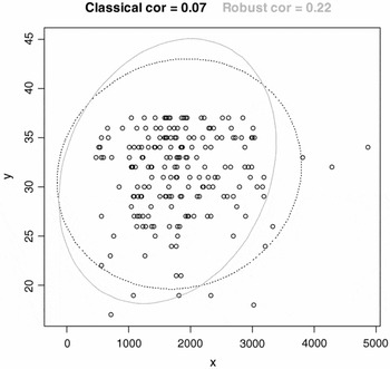
The 95% confidence interval for the correlation coefficient estimate shows that the correlation is not statistical, since it does go through zero. A scatterplot of this data shows that the majority of the data is concentrated in the middle but there do seem to be a number of outlying points (see Figure 2). The robust correlation will objectively calculate a correlation just for the main portion of the data.
Graphic from robust correlation where x = total hours and y = aptitude score

There are a number of choices for robust correlation, but I'm going to use a command from the ‘mvoutlier’ package in R (Gschwandtner & Filzmoser Reference Gschwandtner and Filzmoser2009). This calculates a correlation using robust methods, which the authors specify can be thought of as ‘estimating the mean and covariance of the “good” part of the data’. Appendix D shows how to perform this command using my data, and then shows the actual output. The output shows that the robust correlation is .22. This is somewhat larger than the classical correlation of .07. The difference between the estimates is noticeable and means the correlation may be worth remarking on now, although it would still only explain (R2 = .04) 4% of the variance in scores.
What happens with the robust correlation is that different information has been used in the calculation of the robust correlation versus the classical correlation. This particular command also produces a graphic along with the correlation coefficient that provides a helpful way to see which data was included and which was not (see Figure 2).
As you look at Figure 2 it should be clear that it would be difficult to decide objectively which points are outliers and should be excluded from the robust correlation. The robust correlation used in the mvoutlier library determines the size of the ellipsoid that contains the data in the following way: ‘An observation will be outside of the ellipsoid if its Mahalanobis distance exceeds the 1-alpha quantile of the chi-squared distribution’ (Gschwandtner & Filzmoser Reference Gschwandtner and Filzmoser2009).
You may be concerned that there is no p-value to report along with the correlation. As we saw from the classical output, the p-value is associated with a t-test, and no t-test has been calculated for the robust data (and should not be done just by using a normal t-test, as the calculation would need adjustments because of removing outliers). This does not seem to me to be a problem, as the effect size is much more important than a null significance hypothesis test.
5.3 A robust one-way ANOVA
Last of all, let's look at a one-way ANOVA. I'm using data from an unpublished study I conducted with Japanese people who either lived in the US as children or adults for a period of about 2–4 years, or never lived abroad but were majoring in English at the university level. I call these groups the early-immersionists, the late-immersionists, and the non-immersionists, respectively. I had them produce words beginning with R and L, and then had native speakers rate their accuracy (native speakers also produced the words and were rated as well). I then calculated a percentage accuracy score with both sounds. The mean score for the non-immersionists was M = 81.5 (SD = 18.9), while the late-immersionists had an M = 91.9 (SD = 15.1) and the early-immersionists had the highest mean scores M = 95.2 (SD = 7.4) of any of the Japanese groups. The native speakers of English scored very close to perfect (M = 99.2, SD = 1.2).
A one-way ANOVA performed in R shows that the omnibus ANOVA test is statistical, F (3, 23.3) = 6.3, p = .003, and I conclude that I can go on to look at differences between the individual groups (see Appendix E at http://journals.cambridge.org/lta for the R code and output). R returns a series of confidence intervals for each of the six possible pairings of the four groups. The only confidence interval which does not pass through zero is the last one (see Appendix E), the comparison of the native speakers (NS) to the non-immersionists (those who never studied abroad). This interval is also quite wide, showing that the difference in means between the two groups might be as small as five points or as great as 30 points (the 95% CI is [5.35, 29.9]).
For the robust test, an omnibus ANOVA is not used. Instead, robust comparisons of the pairwise comparisons are done directly (see Appendix E). A 20% means-trimmed percentile bootstrap analysis of the pairwise comparisons reveals only one confidence interval which does not pass through zero, again, that between NS and non-immersionists, [−33, −2.7]. In other words, a robust comparison does not turn up anything different from what was found in the classical one-way ANOVA (and subsequent post-hoc tests).
6. Conclusion
In summary, I have given you some ways to run robust statistics yourself. They are not so very different from how parametric statistics are done, but will give you greater power to find differences between groups. I have demonstrated in several cases here that the conclusions may be different when using robust statistics, but the weight of research shows that the conclusions from robust statistics are more accurate than those of parametric statistics. I hope you will consider the possibility of using robust statistics in your own work.
Acknowledgements
I would like to thank the audience at the 2009 Second Language Research Forum for their responses, which prompted my thinking about this topic, and for the comments from the faculty and students at Penn State. A special thanks to James Lantolf for inviting me to give this talk and clearly being interested in many points of view.
Jenifer Larson-Hall is on the faculty of Kyushu Sangyo University in the Language Education and Research Center, Fukuoka, Japan. She has published articles about the role of age and individual factors in second language acquisition as well as a recent book (Routledge, 2010) about statistics in second language research using SPSS. An online companion to the book, showing how to perform basic classic statistics as well as robust statistics with R, is available on the Routledge website.