1. Introduction
Spatiotemporal correlations quantify how fluctuations in a turbulent flow at one point in space and time relate to those at another. They are central to understanding the mechanisms of turbulence decorrelation, and have broad theoretical and practical relevance (He, Jin & Yang Reference He, Jin and Yang2017). Fundamentally, these correlations provide a means of characterising the temporal evolution of spatial structures, which is essential for the development of turbulence theory. They also underpin a variety of closure models in turbulence, including the direct interaction approximation (Kraichnan Reference Kraichnan1961), the eddy-damped quasi-normal Markovian model (Orszag Reference Orszag1973), and several Eulerian-based closure frameworks (Cambon & Scott Reference Cambon and Scott1999).
Beyond their foundational role in turbulence theory and modelling, spatiotemporal correlations have widespread practical importance across several areas of fluid mechanics. In aeroacoustics, for example, the Lighthill acoustic analogy relates the intensity of sound radiated by turbulent flows to the underlying spatiotemporal structure of velocity fluctuations (Lighthill Reference Lighthill1952). Accurate modelling of these correlations is therefore essential for predicting turbulence-generated noise (Wang, Freund & Lele Reference Wang, Freund and Lele2006). In experimental fluid mechanics, spatiotemporal correlations also play a critical role. Due to the difficulty of simultaneously resolving fine-scale turbulence in both space and time, especially in high-Reynolds-number flows, experimentalists often rely on models to convert between temporal and spatial measurements (Ligrani & Bradshaw Reference Ligrani and Bradshaw1987; Vukoslavĉević et al. Reference Vukoslavĉević, Wallace and Balint1991; Hutchins et al. Reference Hutchins, Nickels, Marusic and Chong2009; Atkinson, Buchmann & Soria Reference Atkinson, Buchmann and Soria2015). For instance, Taylor’s frozen turbulence hypothesis (Taylor Reference Taylor1938) has long been used to infer spatial structures from time-resolved probe data. More refined spatiotemporal models now provide improved mappings that account for decorrelation effects and are increasingly used to interpret particle image velocimetry, hot-wire anemometry and laser Doppler velocimetry data (Del Alamo & Jiménez Reference Del Alamo and Jiménez2009). In this context, models of spatiotemporal correlations help to bridge the gap between limited experimental observables and the full dynamical structure of turbulent flows.
A particularly well-studied quantity in this context is the space–time correlation of streamwise velocity fluctuations in a homogeneous flow direction at statistically stationary conditions. This is commonly defined as
 \begin{align} R_{uu}(r,\tau ) = \langle u'(\boldsymbol{x},t)\, u'(\boldsymbol{x} + r\boldsymbol{e}_1, t + \tau ) \rangle , \end{align}
where
 $ \boldsymbol{e}_1$
is the unit vector in the streamwise direction,
 $ r$
is the spatial separation, and
 $ \tau$
is the temporal lag. For brevity, we denote this as
 $ R(r, \tau )$
. Here,
 $ R(r, \tau )$
does not depend on
 $x$
or
 $t$
because of the assumed spatial homogeneity and temporal stationarity.
A number of models exist for
 $ R(r, \tau )$
. One of the earliest models of space–time correlation is based on Taylor’s frozen turbulence hypothesis (Taylor Reference Taylor1938), which assumes that small-scale turbulent structures are convected unchanged at a mean velocity
 $ U_c$
, such that
 $ R(r, \tau ) = R(r - U_c \tau , 0)$
. While Taylor’s hypothesis captures the dominant convection of eddies, it fails to account for the decorrelation that occurs due to nonlinear interactions, large-scale sweeping, and distortion effects (Dennis & Nickels Reference Dennis and Nickels2008; Moin Reference Moin2009). To address these limitations, He & Zhang (Reference He and Zhang2006) introduced the elliptic approximation (EA), which incorporates not only mean convection but also turbulent sweeping and distortion. The EA, derived from a Taylor series expansion of the space–time correlation function, combines the frozen flow hypothesis, Kolmogorov’s similarity scaling (Kolmogorov Reference Kolmogorov1941, Reference Kolmogorov1991), and the Kraichnan–Tennekes random sweeping framework (Kraichnan Reference Kraichnan1964; Tennekes Reference Tennekes1975). It relates space–time correlations to spatial correlations through an effective elliptical mapping defined by two characteristic velocities: a convection velocity governed by the local mean flow, and a sweeping velocity associated with turbulence intensity and shear rate (Zhao & He Reference Zhao and He2009). Other approaches have also been proposed. For example, Wilczek & Narita (Reference Wilczek and Narita2012) derived a random advection model incorporating mean flow based on Kraichnan’s random sweeping hypothesis, yielding wavenumber–frequency spectra expressed as the instantaneous energy spectrum multiplied by a Gaussian frequency distribution. Wilczek et al. (Reference Wilczek, Stevens and Meneveau2015a
,
Reference Wilczek, Stevens and Meneveaub
) demonstrated that the model captures essential features – Doppler shift and Doppler broadening – and established good agreement with numerical simulation data in the logarithmic layer of turbulent channel flows. And de Maré & Mann (Reference de Maré and Mann2016) developed a spatiotemporal model by combining the Mann model (Mann Reference Mann1994) with Kristensen’s longitudinal coherence framework (Kristensen Reference Kristensen1979), applicable to high-Reynolds-number turbulence. Lukassen et al. (Reference Lukassen, Stevens, Meneveau and Wilczek2018) derived an analytical model based on the random sweeping hypothesis, expressing space–time correlations as a convolution of the spatial correlation with a temporal decorrelation kernel. Their model aligns with the classical Kovasznay–Corrsin conjecture (Phillips Reference Phillips2000). Towne, Lozano-Durán & Yang (Reference Towne, Lozano-Durán and Yang2020) developed a resolvent-based estimation method to infer space–time flow statistics from limited known data, demonstrating its effectiveness in estimating flow characteristics in a low-Reynolds-number turbulent channel flow. Following Towne et al. (Reference Towne, Lozano-Durán and Yang2020), Yang et al. (Reference Yang, Jin, Wu, Yang and He2020) systematically evaluated the performance of the resolvent-based estimation method, and found that the space–time energy spectra predicted are sensitive to the location of the reference plane. For comprehensive reviews of spatiotemporal correlations and modelling techniques, the reader is referred to Favre (Reference Favre1965), Wallace (Reference Wallace2014), He et al. (Reference He, Jin and Yang2017) and Wu & He (Reference Wu and He2021a
).
We consider the EA, which has been validated in a range of turbulent flows, including channel flows (He & Zhang Reference He and Zhang2006; Zhao & He Reference Zhao and He2009), turbulent Rayleigh–Bénard convection (He, He & Tong Reference He, He and Tong2010; He & Tong Reference He and Tong2011; Zhou et al. Reference Zhou, Li, Lu and Liu2011), round jet (Zhang, Wan & Sun Reference Zhang, Wan and Sun2019) and turbulent boundary layers (Wang, Guan & Jiang Reference Wang, Guan and Jiang2014). Despite its success, several open questions remain regarding the applicability and theoretical foundations of the model. First, EA – like Taylor’s hypothesis – assumes a constant convection velocity across the entire space–time domain. However, this assumption becomes increasingly inaccurate at large spatial separations and time delays. As the contribution from small-scale eddies diminishes with increasing
 $ r$
and
 $ \tau$
, large-scale motions become dominant, and these possess different convection velocities. Del Alamo & Jiménez (Reference Del Alamo and Jiménez2009) observed that small-scale eddies tend to convect with the local mean velocity, whereas larger, global modes travel at a nearly uniform speed proportional to the bulk flow velocity in channel flow. Second, the theoretical basis of the EA rests on assumptions that are strictly valid only within the inertial subrange. Specifically, the Kolmogorov similarity hypothesis (Kolmogorov Reference Kolmogorov1941, Reference Kolmogorov1991) provides the inertial-range scaling for the spatial energy spectrum, whereas the Kraichnan–Tennekes random sweeping hypothesis (Kraichnan Reference Kraichnan1964; Tennekes Reference Tennekes1975) utilises this energy spectrum to derive the corresponding Eulerian frequency spectrum. Here, the random sweeping hypothesis does not assume inertial range, but due to Kolmogorov’s similarity hypothesis, which assumes inertial range, the resulting Eulerian frequency spectrum is applicable to the inertial range only. Nevertheless, the EA often remains effective even at scales where viscous effects are non-negligible – a fact that lacks a clear theoretical explanation. Third, although the applicability of the EA has been extended to passive scalars (He et al. Reference He, He and Tong2010; He & Tong Reference He and Tong2011, Reference He and Tong2014), existing discussions and validations of the EA are largely restricted to incompressible flows. Whether the model remains valid under compressible conditions, particularly at finite Mach numbers, has not been systematically explored.
This study addresses these open questions. We show that deviations from elliptic iso-correlation contours – termed ‘non-elliptic effects’ – in the viscous sublayer are attributable to viscous effects. A correction is proposed to account for these effects. Additionally, we demonstrate that the effectiveness of the EA does not hinge on strict inertial-range scaling; rather, it depends on the presence of extended self-similarity (ESS) between spatial and temporal correlations. Finally, we evaluate the applicability of the EA in compressible turbulence. We find that the model remains valid for describing the spatiotemporal correlations of both velocity and temperature fluctuations at finite Mach numbers.
The remainder of this paper is organised as follows. In § 2, we revisit the theoretical derivation of the EA. The details of the direct numerical simulations (DNS) used in this study are provided in § 3. We then evaluate the key assumptions underlying the EA: in § 4.1, we examine deviations from ellipticity and propose a correction; in § 4.2, we test the Eulerian frequency spectrum derived from Kraichnan–Tennekes random sweeping hypothesis. The model’s validity under compressible conditions is explored in § 4.3. Finally, conclusions are drawn in § 5.
2. The EA model
For completeness and to support the discussion in § 4, we summarise the EA and its derivation. Only the key steps are presented here; for detailed derivations, the reader is referred to He & Zhang (Reference He and Zhang2006) and Zhao & He (Reference Zhao and He2009).
Following He & Zhang (Reference He and Zhang2006), the starting point is a Taylor expansion of the space–time correlation function
 $ R(r,\tau )$
about
 $ r = 0$
,
 $ \tau = 0$
:
 \begin{align} R(r,\tau ) = R_0 + \left .\frac {\partial R}{\partial r}\right |_0 r + \left .\frac {\partial R}{\partial \tau }\right |_0 \tau + \left .\frac {\partial ^2 R}{\partial r\, \partial \tau }\right |_0 r \tau + \frac {1}{2}\left [ \left .\frac {\partial ^2 R}{\partial r^2}\right |_0 r^2 + \left .\frac {\partial ^2 R}{\partial \tau ^2}\right |_0 \tau ^2 \right ] + \cdots , \end{align}
where the subscript 0 indicates evaluation at
 $ r = 0$
,
 $ \tau = 0$
. Due to the assumed spatial homogeneity and temporal stationarity, the first derivatives vanish:
 $ \partial _r R|_0 = 0$
and
 $ \partial _\tau R|_0 = 0$
. Turbulence loses coherence over both space distance and time delay. Consider a spatial separation
 $ r_c$
such that the correlation at
 $ (r_c, 0)$
equals that at
 $ (r, \tau )$
:
 \begin{align} R(r,\tau ) = R(r_c, 0). \end{align}
Expanding the right-hand side yields
 \begin{align} R(r,\tau ) = R_0 + \left .\frac {\partial ^2 R}{\partial r^2}\right |_0 r_c^2 + \cdots . \end{align}
Comparing (2.1) and (2.3) up to second-order terms gives
 \begin{align} r_c^2 = (r - U\tau )^2 + (V\tau )^2, \end{align}
where
 \begin{align} U = -\left .\frac {\partial ^2 R}{\partial r\, \partial \tau }\right |_0 \left [\left .\frac {\partial ^2 R}{\partial r^2}\right |_0\right ]^{-1} \end{align}
is the convection velocity, and
 \begin{align} V^2 = \left .\frac {\partial ^2 R}{\partial \tau ^2}\right |_0 \left [\left .\frac {\partial ^2 R}{\partial r^2}\right |_0\right ]^{-1} - U^2 \end{align}
is the sweeping velocity. Substituting (2.4) into (2.2) leads to
 \begin{align} R(r,\tau ) = R\left ( \sqrt {(r - U\tau )^2 + (V\tau )^2}, 0 \right ), \end{align}
which implies that space–time correlations decay across elliptical contours – hence the term ‘elliptic approximation’. However, the derivation is strictly valid only for infinitesimal
 $ r$
and
 $ \tau$
.
Extending the EA to finite separations is non-trivial. A necessary (though not sufficient) condition is that the intercepts of a constant-
 $ R$
contour on the
 $ r$
- and
 $ \tau$
-axes maintain a constant ratio. Zhao & He (Reference Zhao and He2009) verified this condition by invoking Taylor’s frozen turbulence hypothesis (Taylor Reference Taylor1938), Kolmogorov’s similarity hypothesis (Kolmogorov Reference Kolmogorov1941, Reference Kolmogorov1991) and the Kraichnan–Tennekes random sweeping hypothesis (Kraichnan Reference Kraichnan1964; Tennekes Reference Tennekes1975). First, according to Kolmogorov’s theory and the random sweeping hypothesis, the second-order velocity structure function
 \begin{align} D(r,\tau ) = \left \langle \left | u_1^{\prime }(x_1 + r, t + \tau ) - u_1^{\prime }(x_1, t) \right |^2 \right \rangle \end{align}
has the following inertial-range scalings:
 \begin{align} D(r, 0) &= C_{\!K} (\epsilon r)^{2/3}, \end{align}
 \begin{align} D(0, \tau ) &= C_{\!K} (\epsilon V_c \tau )^{2/3}, \end{align}
where
 $ C_{\!K}$
is a constant,
 $ \epsilon$
is the dissipation rate of turbulent kinetic energy, and
 $ V_c$
is a characteristic (constant) velocity. The structure function is related to the space–time correlation via
 \begin{align} D(r, 0) &= 2 R(0,0) - 2 R(r,0), \\[-9pt] \nonumber \end{align}
 \begin{align} D(0, \tau ) &= 2 R(0,0) - 2 R(0,\tau ). \end{align}
Next, let
 $ r_c$
and
 $ \tau _c$
denote the spatial and temporal intercepts of a constant-
 $ R$
contour:
 \begin{align} R(r_c, 0) = R(0, \tau _c). \end{align}
Finally, (2.9)–(2.13) together give
 \begin{align} C_{\!K} (\epsilon r_c)^{2/3} = C_{\!K} (\epsilon V_c \tau _c)^{2/3}, \end{align}
which simplifies to
 \begin{align} \frac {r_c}{\tau _c} = V_c, \end{align}
indicating that the ratio of spatial to temporal separation at equal correlation is constant in the inertial range.
To summarise, the EA in (2.7) provides a framework for relating temporal measurements at a single point to spatial correlations across the flow field. The model requires knowledge of two parameters: the convection velocity
 $U$
, and the sweeping velocity
 $V$
. In the original formulation, Zhao & He (Reference Zhao and He2009) proposed estimating
 $U$
from the local mean velocity, while
 $V$
accounts for both shear-induced and random sweeping effects.
While the EA provides an approximation of space–time correlations using spatial correlations alone, two questions remain unresolved. First, the EA relies on inertial-range scaling arguments, which break down in the viscous sublayer. Second, the model was derived under the assumption of incompressibility. Its applicability to compressible flows at finite Mach numbers – where dilatational effects and acoustic modes may alter the correlation structure – is not well understood. These concerns motivate a closer examination of the model’s validity in both near-wall and compressible regimes.
3. The DNS details
3.1. Governing equations
The compressible Navier–Stokes equations are solved in a plane channel. The equations are written in index notation, with summation implied over repeated indices:
 \begin{align} \frac {\partial \tilde {\rho }}{\partial t} + \frac {\partial (\tilde {\rho } \tilde {u}_{\!j})}{\partial x_{\!j}} &= 0, \end{align}
 \begin{align} \frac {\partial (\tilde {\rho } \tilde {u}_i)}{\partial t} + \frac {\partial (\tilde {\rho } \tilde {u}_i \tilde {u}_{\!j})}{\partial x_{\!j}} &= -\frac {\partial \tilde {p}}{\partial x_i} + \frac {\partial \tilde {\sigma }_{\textit{ij}}}{\partial x_{\!j}} + f_i \delta _{i1}, \end{align}
 \begin{align} \frac {\partial (\tilde {\rho } \tilde {E})}{\partial t} + \frac {\partial (\tilde {\rho } \tilde {E} \tilde {u}_{\!j})}{\partial x_{\!j}} &= -\frac {\partial (\tilde {p} \tilde {u}_{\!j})}{\partial x_{\!j}} + \frac {\partial (\tilde {u}_i \tilde {\sigma }_{\textit{ij}})}{\partial x_{\!j}} - \frac {\partial \tilde {q}_{\!j}}{\partial x_{\!j}} + f_1 \tilde {u}_1 - \phi , \end{align}
where
 \begin{align} \tilde {\sigma }_{\textit{ij}} = 2\tilde {\mu } \tilde {S}_{\textit{ij}} - \frac {2}{3} \tilde {\mu } \tilde {S}_{kk} \delta _{\textit{ij}}, \quad \tilde {E} = C_V \tilde {T} + \frac {1}{2} \tilde {u}_i \tilde {u}_i, \quad \tilde {q}_{\!j} = -\tilde {\kappa } \frac {\partial \tilde {T}}{\partial x_{\!j}}. \end{align}
Here,
 $\tilde {u}_i$
is the
 $i$
th component of velocity in the Cartesian coordinate system
 $x_i$
,
 $t$
is time,
 $\tilde {p}$
is the thermodynamic pressure,
 $\tilde {\sigma }_{\textit{ij}}$
is the viscous stress tensor,
 $f_i$
is a uniform body force driving the flow (applied only in the streamwise direction),
 $\tilde {E}$
is the total energy per unit mass,
 $\tilde {q}_{\!j}$
is the heat flux vector, and
 $\phi$
represents a heat source term. The material properties include the dynamic viscosity
 $\tilde {\mu }$
, thermal conductivity
 $\tilde {\kappa }$
, and specific heat at constant volume
 $C_V$
. The molecular Prandtl number is defined as
 ${{Pr}} = C_p \tilde {\mu } / \tilde {\kappa }$
and is set to 0.72 in the present simulations. Temperature dependence of the viscosity is modelled using Sutherland’s law:
 \begin{align} \tilde {\mu } = \mu _{\textit{ref}} \left ( \frac {\tilde {T}}{T_{\textit{ref}}} \right )^{3/2} \frac {T_{\textit{ref}} + S}{\tilde {T} + S}, \end{align}
where
 $\mu _{\textit{ref}}$
is the reference viscosity at reference temperature
 $T_{\textit{ref}}$
, and
 $S = 110.4$
K is Sutherland’s constant. The ideal gas law is used to close the system:
 \begin{align} \tilde {p} = \tilde {\rho } R \tilde {T}, \end{align}
where
 $R$
is the specific gas constant.
3.2. Computational set-up
The details of the DNS are summarised in table 1. The nomenclature of the cases follows the format M
 $[10\times U_{{m}}/a_{\textit{ref}}]$
R
 $[{\textit{Re}}/1000]$
k. The bulk Reynolds number, Mach number, bulk Mach number and friction Reynolds number define the flow condition and are
 \begin{align} {{\textit{Re}}} = \frac {\rho _m U_m H}{\mu _{{w}}}, \quad {{\textit{Ma}}} = \frac {U_m}{a_{\textit{ref}}}, \quad {{\textit{Ma}}_b} = \frac {U_m}{a_m}, \quad {{\textit{Re}}}_\tau = \frac {\sqrt {\tau _w \rho _w}\, H}{\mu _w}, \end{align}
with
 \begin{align} \rho _m = \frac {1}{H} \int _0^H \langle \tilde {\rho } \rangle \, {\rm d}y, \quad U_m = \frac {1}{\rho _m H} \int _0^H \langle \tilde {\rho } \tilde {u}_1 \rangle \, {\rm d}y. \end{align}
Computational parameters for the DNS. The suffix ‘k’ in case nomenclature denotes ‘thousands’ (kilo). The asterisk in the case M80R27k* indicates that this configuration incorporates a heating source term
 $\phi$
to maintain a prescribed bulk temperature, with wall temperature
 $10.09 T_{\textit{ref}}$
, distinguishing it from other cases in the study. Grid resolution is characterised using three scalings. Wall-unit scaling (normalised by
 $\mu _w/\sqrt {\rho _w\tau _w}$
) is given by
 $\Delta x^+, \Delta y_w^+, \Delta y_c^+, \Delta z^+$
. Semi-local scaling (normalised by
 $\mu /\sqrt {\rho \tau _w}$
) is represented by
 $\Delta x^*, \Delta z^*$
for the largest spacings in the streamwise and spanwise directions, and by
 $\Delta y_w^*, \Delta y_c^*$
for spacings at the wall and channel centreline, respectively. Kolmogorov scaling is indicated by
 $\Delta x/\eta , \Delta z/\eta$
for the largest spacings, and
 $\Delta y_w/\eta _w, \Delta y_c/\eta _c$
for spacings at the wall and centreline. Here,
 $\theta = (T_w - T_b)/(T_r - T_b)$
denotes the wall temperature parameter, with
 $T_r = T_e(1+0.5(\gamma -1)rM_e^2)$
being the recovery temperature, and
 $-B_q = -q_w/(\rho _wC_pu_{\tau }T_w)$
is the heat flux coefficient.

Here,
 $H$
is the channel half-height, the subscript
 $m$
denotes a volume-averaged quantity,
 $w$
indicates values at the wall,
 $a_{\textit{ref}}$
is the speed of sound at the reference temperature, and
 $a_{{m}}$
is the speed of sound at the bulk temperature.
The computational domain has dimensions
 $ 4\pi H \times 2H \times 2\pi H$
, which is larger than the minimal channel used in earlier studies (Flores & Jiménez Reference Flores and Jiménez2010; Lozano-Durán & Jiménez Reference Lozano-Durán and Jiménez2014). Domains of similar size have been employed in previous simulations of compressible channel flow (Coleman, Kim & Moser Reference Coleman, Kim and Moser1995; Morinishi, Tamano & Nakabayashi Reference Morinishi, Tamano and Nakabayashi2004; Chen et al. Reference Chen, Huang, Shi, Yang and Lv2022). Grid points are clustered in the wall-normal (
 $ y$
) direction and uniformly distributed in the streamwise (
 $ x$
) and spanwise (
 $ z$
) directions. The first off-wall grid point satisfies
 $ \Delta y_w^+ \leqslant 0.5$
, and the wall-normal spacing at the channel centreline is
 $ \Delta y_c^+ \lesssim 7.2$
. The streamwise and spanwise grid spacings are
 $ \Delta x^+ \lesssim 8$
and
 $ \Delta z^+ \lesssim 5.5$
, respectively. These resolutions comply with established DNS guidelines (Kim, Moin & Moser Reference Kim, Moin and Moser1987; Oliver et al. Reference Oliver, Malaya, Ulerich and Moser2014) and align with those used in recent compressible flow simulations (Modesti, Bernardini & Pirozzoli Reference Modesti, Bernardini and Pirozzoli2015; Yao & Hussain Reference Yao and Hussain2020; Zhang, Song & Xia Reference Zhang, Song and Xia2023). Grid resolution is also reported in two additional scalings: semi-local units and Kolmogorov scaling. The largest grid spacings scaled by semi-local units are
 $\Delta x^* = 48.0$
and
 $\Delta z^* = 32.7$
in the streamwise and spanwise directions, respectively. These relatively large values result from the low temperature at the channel centreline – a situation that has been observed in hypersonic boundary layer flows (Zhang, Duan & Choudhari Reference Zhang, Duan and Choudhari2018; Huang, Duan & Choudhari Reference Huang, Duan and Choudhari2022). Nevertheless, the grid resolution remains well within the grid resolution requirements for DNS, as is clear when it is expressed in Kolmogorov units. Although finer grids are necessary to capture rare intermittent events, the present resolution is sufficient to accurately resolve first- and second-order statistics (Yang et al. Reference Yang, Hong, Lee and Huang2021; Chen et al. Reference Chen, Zhu, Shi and Yang2023), which are the primary focus of this study.
The boundary conditions are periodic in the streamwise (
 $x$
) and spanwise (
 $z$
) directions. The walls are no-slip and isothermal. The wall temperature is set to
 $T_{{w}} = T_{\textit{ref}}$
for all cases except M80R27k*, which uses tailored wall temperature
 $10.09 T_{\textit{ref}}$
. The reference temperature is
 $T_{\textit{ref}} = 273\,\mathrm{K}$
for all cases except M80R27k*, where it is
 $100\,\mathrm{K}$
. We set
 $H = 1$
and
 $\rho _m = 1$
in our DNS, and vary the viscosity
 $\mu _{{w}}$
and the driving force
 $f_1$
to control the Reynolds number
 ${\textit{Re}}$
and the Mach number
 ${\textit{Ma}}$
. In this channel configuration, all viscous heating is removed through the walls, resulting in a mean temperature gradient from the wall to the centre of the channel. At high Mach numbers, this gradient can significantly raise the centreline temperature, thereby increasing the viscosity and potentially causing relaminarisation. To mitigate this effect, we follow the work of Yu et al. (Reference Yu, Xu and Pirozzoli2019, Reference Yu, Xu and Pirozzoli2020) and introduce a cooling source term
 $\phi$
in the energy equation (3.3) to regulate the bulk temperature. For case M80R27k*, the bulk temperature is set to
 $T_b/T_{\textit{ref}} = 3.272$
. The relevant aerodynamic heating parameters are also summarised in table 1. For each case, the heat flux coefficient
 $-B_q=-q_w/ (\rho _wC_pu_\tau T_w )$
and wall temperature parameter
 $\theta = (T_w-T_b )/ (T_r-T_b )$
are reported. Here,
 $T_r=T_e (1+0.5 (\gamma -1 )r M_e^2 )$
denotes the recovery temperature, with
 $r=0.89$
being the recovery factor, and the subscript
 $e$
referring to properties at the channel centreline. In the four cases without cooling,
 $\theta$
exhibits negative values due to the bulk temperature exceeding the wall temperature. In contrast, case M80R27k* shows the opposite behaviour, with significant cooling causing the bulk temperature to fall below the wall temperature. The heat flux coefficient generally increases with Mach number among the four typical cases without cooling, reaching the value 0.132 in case M30R05k. However, in case M80R27k*, this coefficient is even lower than that in the lower-Mach-number case M30R05k.
Calculations are performed using the OpenCFD-SC solver (Li et al. Reference Li, Fu, Ma and Liang2010), a high-order finite-difference code validated for compressible turbulence. Further details of the solver are available in previous studies (Liang & Li Reference Liang and Li2015; Xu et al. Reference Xu, Wang, Wan, Yu, Li and Chen2021; Yu & Xu Reference Yu and Xu2021; Zhang et al. Reference Zhang, Song and Xia2023). Here, we briefly summarise its key features. Convective terms are discretised using a seventh-order weighted essentially non-oscillatory (WENO) scheme, and viscous terms with an eighth-order central difference scheme, and time integration is performed using a third-order explicit Runge–Kutta method. To ensure numerical stability at high Mach numbers, explicit filtering is applied to remove high-wavenumber oscillations (Bogey & Bailly Reference Bogey and Bailly2004; Li, Fu & Ma Reference Li, Fu and Ma2006).
A total of 500 flow field snapshots are collected at intervals of
 $ 0.05H/U_m$
, providing sufficiently fine temporal resolution to enable accurate analysis of spatiotemporal correlations. This temporal resolution has been demonstrated to be effective in previous studies (He & Zhang Reference He and Zhang2006; Wu & He Reference Wu and He2021b
; Yang & Yang Reference Yang and Yang2022). Although the spatiotemporal correlation is defined in physical space, we leverage the periodicity in the streamwise direction to accelerate computations using fast Fourier transforms.
3.3. Flow statistics
Although the primary focus of this study is the spatiotemporal correlation of turbulence, we first present mean flow statistics to provide context for interpreting compressibility and Mach number effects.
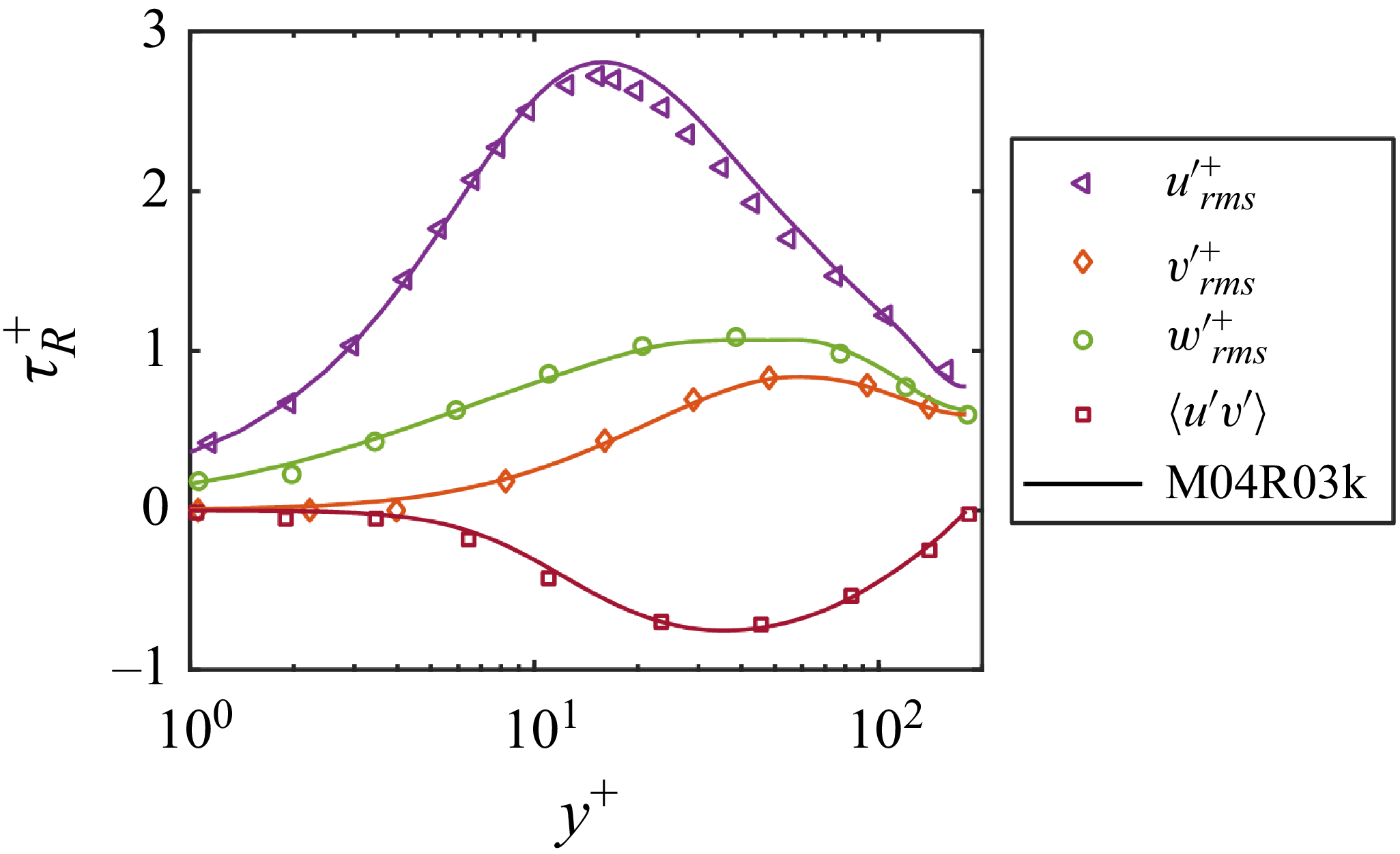
Figure 1(a) shows the mean velocity profiles for all simulated cases. The
 $Re_\tau = 180$
incompressible channel flow (Modesti & Pirozzoli Reference Modesti and Pirozzoli2016) is also included for comparison. Case M04R03k, which is at the friction Reynolds number 180, closely follows the incompressible profile. As the Mach number increases, the mean velocity profiles progressively deviate from the incompressible law of the wall – except in case M80R27k*. Despite its high Mach number, M80R27k* exhibits a profile that remains relatively close to the incompressible reference. Figure 1(b) presents the corresponding mean temperature distributions. In cases without cooling, higher Mach numbers result in a stronger temperature difference between the channel centreline and the wall. This temperature contrast increases from
 $(T_c - T_w)/T_w = 0.02$
in M04R03k to
 $1.5$
in M30R05k. By contrast, M80R27k* – due to the presence of a cooling source – exhibits an inverted temperature profile, with the centreline temperature lower than that at the wall. Figure 1(c,d) display the turbulent Mach number
 $M_t$
and fluctuating Mach number
 $M'$
, respectively, defined as
 \begin{align} M_t = \frac {\langle u'_i u'_i \rangle ^{1/2}}{\langle c \rangle }, \quad M' = \sqrt {\left\langle \left( \frac {\sqrt {\tilde {u}_i \tilde {u}_i}}{c} - \left \langle \frac {\sqrt {\tilde {u}_i \tilde {u}_i}}{c} \right \rangle \right)^2 \right\rangle }. \end{align}
(a) Mean velocity profiles. (b) Mean temperature profiles. (c) Turbulent Mach number. (d) Fluctuating Mach number. The black symbols in (a) are reference incompressible channel flow data at
 ${{\textit{Re}}}_\tau = 180$
(Modesti & Pirozzoli Reference Modesti and Pirozzoli2016).

These metrics characterise the intensity of turbulent fluctuations relative to the local speed of sound
 $c$
. Both
 $M_t$
and
 $M'$
increase with Mach number, as expected. For cases without cooling, their spatial distributions are similar: peak magnitudes and locations align, and shift away from the wall with increasing Mach number. M80R27k* again shows distinct behaviour –
 $M_t$
peaks at approximately 0.5 in the buffer layer (
 $y^+ \approx 18$
), and
 $M'$
exhibits a secondary peak in the outer region. This secondary peak, though uncommon in channel flows (Zhang et al. Reference Zhang, Song and Xia2023), has been reported in hypersonic turbulent boundary layers (Duan, Beekman & Martin Reference Duan, Beekman and Martin2011). Finally, note that in M04R03k, both
 $M_t$
and
 $M'$
remain below 0.05, indicating negligible compressibility effects. This is further corroborated in figure 2, which shows that the root mean square fluctuating velocity and Reynolds shear stress profiles closely match those of the incompressible reference.
The distributions of root mean square fluctuating velocity and Reynolds shear stress for case M04R03k (lines) and its strictly incompressible counterpart (symbols) at friction Reynolds number
 $Re_\tau = 180$
(Modesti & Pirozzoli Reference Modesti and Pirozzoli2016).

We also present a budget analysis for the energy. For a plane channel, the ensemble-averaged energy equation (3.3) simplifies to
 \begin{align} \frac {\partial \langle -\tilde {\rho } u_i^{\prime \prime } h_0^{\prime \prime } \rangle }{\partial x_i} + \left \langle \tilde {u}_{\!j} \frac {\partial \tilde {\sigma }_{\textit{ij}}}{\partial x_i} \right \rangle + \left \langle \tilde {\sigma }_{\textit{ij}} \frac {\partial \tilde {u}_i}{\partial x_{\!j}} \right \rangle + \frac {\partial \langle -\tilde {q}_i \rangle }{\partial x_i} + \langle f_1 \tilde {u}_1 \rangle + \langle -\phi \rangle = 0, \end{align}
where
 $h_0^{\prime \prime }$
is the fluctuation of total enthalpy. In the near-wall region, the energy balance is dominated by the interplay between viscous dissipation and wall heat conduction, which nearly offset each other. In the buffer layer, the dynamics becomes more complex as turbulent transport and viscous work both contribute appreciably to the energy transfer. Further away, in the outer layer, the balance depends on the cooling condition: without cooling, the body force work is mainly compensated by turbulent total enthalpy transport, whereas with cooling, it is offset by both the imposed cooling and turbulent transport.
Energy budget analysis for (a) M04R03k, (b) M08R03k, (c) M15R03k, (d) M30R05k and (e) M80R27k*. All terms are normalised by
 $\rho _m U_m^3 / H$
.

4. Results
We assess the EA as defined in (2.7), and revisit its derivation. The convection velocity
 $U$
and sweeping velocity
 $V$
in (2.7) are extracted directly from DNS data, in contrast to Zhao & He (Reference Zhao and He2009), who derived analytical expressions of these parameters from the Navier–Stokes equations under high-Reynolds-number, isotropic turbulence assumptions. Our approach allows us to isolate and evaluate the structural validity of the model itself.
This rest of this section is organised as follows. In § 4.1, we evaluate the assumption of a constant convection velocity at large spatial and temporal separations, demonstrating that
 $U$
becomes scale-dependent due to shear effects. A correction is proposed to account for this variation. In § 4.2, we examine the validity of the inertial-range scalings in (2.9) and (2.10). Although these scalings break down near the wall, we show that the EA remains valid due to the presence of ESS. Finally, in § 4.3, we test the applicability of the EA to compressible flows and temperature fluctuations at finite Mach numbers. We find that the correction introduced in § 4.1 remains effective, and that ESS continues to hold for both velocity and temperature correlations under compressible conditions.
4.1. Convection velocity
The EA, like Taylor’s hypothesis, assumes a constant convection velocity across all scales. To evaluate this assumption, we examine the spatiotemporal correlation structure in the low-Mach-number case M04R03k, focusing on the viscous sublayer and regions of large spatial separation
 $ r$
and time delay
 $ \tau$
.
If the convection velocity were truly constant, then the principal axes of the iso-correlation contours would exhibit uniform inclination angles across all values of
 $ \tau ^+$
. Equivalently, for a time delay
 $ \tau ^+$
, the peak location
 $ \Delta x^+_p$
of the correlation function
 $ R(\Delta x^+, \tau ^+)$
would scale linearly with
 $ \tau ^+$
.
Figure 4(a–c,f–h) illustrate this behaviour in the near-wall region (
 $ y^+ = 1.9, 5.1,\,17.7$
). At small
 $ \tau ^+$
, the peak displacement
 $ \Delta x^+_p$
varies linearly with
 $ \tau ^+$
(figure 4
f–h), consistent with a constant convection velocity at short time delays. However, at larger
 $ \tau ^+$
, the iso-correlation contours tilt progressively towards the
 $ \Delta x^+$
-axis (figure 4
a–c), indicating an apparent increase in convection velocity over time. This deviation arises because Taylor’s hypothesis assumes that advection dominates the evolution of turbulent structures; but additional mechanisms – such as convective acceleration, pressure gradients and viscous diffusion – become significant near the wall (Geng et al. Reference Geng, He, Wang, Xu, Lozano-Durán and Wallace2015). These effects contribute to the breakdown of the constant convection velocity assumption in the near-wall region.
Spatiotemporal correlation in the low-Mach-number case M04R03k. (a–e) Iso-correlation contours at five wall-normal locations: (a,f)
 $ y^+ = 1.9$
, (b,g)
 $ y^+ = 5.1$
, (c,h)
 $ y^+ = 17.7$
, (d,i)
 $ y^+ = 87.7$
, and (e,j)
 $ y^+ = 180.2$
. Dashed lines indicate the inclination of the principal axis near the origin. (f–j) Evolution of the correlation peak location
 $ \Delta x^+_p$
with increasing
 $ \tau ^+$
at corresponding wall-normal positions. The Taylor hypothesis assumes constant convection velocity, whereas the present study employs the modified convection velocity defined in (4.3). Contour levels are
 $ R = 0.8,\, 0.6,\, 0.4,\, 0.2$
.

Figure 4(d,e,i,j) show results for the logarithmic and outer layers (
 $ y^+ = 87.7,\,180.2$
). Here, the contour orientation remains largely invariant with
 $ \tau ^+$
, and the peak position
 $ \Delta x^+_p$
scales linearly with
 $ \tau ^+$
, consistent with a constant convection velocity. These observations support the validity of the assumption that the influence of viscous and shear effects is small.
The breakdown of the constant convection velocity in the viscous sublayer is attributed to strong shear and viscous effects. Del Alamo & Jiménez (Reference Del Alamo and Jiménez2009) formulated the convection velocity as a weighted integral of the phase velocity across wavenumbers:
 \begin{align} U \sim \int c_u(k)\, |\hat {u}(k)|^2\, k^2\, {\rm d}k. \end{align}
This implies convection is dominated by high-wavenumber modes – which decorrelate faster than low-wavenumber modes (Sanada & Shanmugasundaram Reference Sanada and Shanmugasundaram1992) – causing their spectral contribution to the correlation to diminish rapidly. Consequently, the convection velocity exhibits spatiotemporal variation due to significant phase-velocity differences between high- and low-wavenumber modes near the wall (Del Alamo & Jiménez Reference Del Alamo and Jiménez2009). To account for this, we introduce a shear-induced acceleration
 $ a_S$
. By dimensional analysis, this acceleration can only depend on the kinematic viscosity
 $ \nu$
and the local mean shear
 $ \partial \langle \tilde {u}_1 \rangle / \partial y$
in the wall layer, and is
 \begin{align} a_S = C\left [\nu \left (\frac {\partial \langle \tilde {u}_1 \rangle }{\partial y}\right )^3\right ]^{1/2}, \end{align}
where
 $ C = 0.021$
is a model constant obtained from DNS. The modified convection velocity is then given by
 \begin{align} U_c = U + a_S\, |\tau |, \end{align}
where
 $ U$
is the base convection velocity defined in (2.5), and
 $ U_c$
incorporates shear-induced effects. Equation (4.3) implies that this correction is most significant in the viscous sublayer, where the shear rate is highest. To evaluate the proposed correction, we compare DNS measurements of the peak correlation location
 $ \Delta x^+_p$
with predictions from both the original EA and the modified formulation in (4.3), across wall-normal positions
 $ y^+ = 1.9$
,
 $ 5.1$
,
 $ 17.7$
,
 $ 87.7$
and
 $ 180.2$
. Results are shown in figure 4(f–j). In the near-wall region (low
 $ y^+$
), the modified model more accurately captures the delayed shift of the correlation peak at large
 $ \tau ^+$
, outperforming the original EA formulation. This highlights the role of shear-induced acceleration in improving spatiotemporal correlation predictions near the wall. Additional validation under compressible conditions is presented in § 4.3.
We wish to emphasise that the objective of this section is not to propose a superior alternative to the existing EA model, but to identify and verify the physical mechanism that limits the standard model’s accuracy in capturing peak shifts. The proposed correction serves to validate this physical insight, while maintaining the established EA framework. It should also be noted that the present model does not distinguish between turbulent scales. Scale-dependent analyses can be found in e.g. Wills (Reference Wills1964) and Del Alamo & Jiménez (Reference Del Alamo and Jiménez2009). Wills (Reference Wills1964) examined wavelength-dependent convection velocities using space–time energy spectra, while Del Alamo & Jiménez (Reference Del Alamo and Jiménez2009) proposed a method for estimating the convection velocity of individual modes in turbulent shear flows based on temporal information and derivatives of the velocity signal. These approaches offer a more detailed characterisation of scale-dependent convection. However, compared to spatiotemporal correlation models such as Taylor’s hypothesis and the EA, they require more extensive calibration and therefore are outside the current scope of the paper.
Second-order streamwise velocity structure functions for the low-Mach-number case M04R03k. (a) Spatial structure function
 $D_{11}(r_x, \tau =0)$
pre-multiplied by
 $(\epsilon r_x)^{-2/3}$
. (b) Temporal structure function
 $D_{11}(r_x=0, \tau )$
pre-multiplied by
 $(\epsilon V_c \tau )^{-2/3}$
. The dashed lines in (a,b) correspond to
 $C_{\!K} = 2$
(Pope Reference Pope2001). (c) Temporal structure function re-plotted using
 $r_x/V_c$
as the abscissa and compared to the spatial structure function. The dashed line denotes identity.

4.2. Revisiting (2.9) and (2.10)
As outlined in § 2, the validity of the EA at finite spatial separations and temporal delays relies on the inertial-range scalings of the second-order structure functions in (2.9) and (2.10). These scalings are traditionally associated with Kolmogorov’s similarity hypothesis and the Eulerian frequency spectrum derived from the Kraichnan–Tennekes random sweeping hypothesis. In this subsection, we re-examine both scalings and demonstrate that although neither holds strictly across extended ranges, the EA remains valid due to the presence of ESS.
We focus again on the low-Mach-number case M04R03k. Figure 5(a) shows the spatial second-order streamwise velocity structure function, pre-multiplied by
 $ (\epsilon r_x)^{-2/3}$
. Similarly, figure 5(b) shows the temporal structure function, pre-multiplied by
 $ (\epsilon V_c \tau )^{-2/3}$
, where
 $V_c$
is the characteristic velocity in (2.10), and
 $ u_\eta = (\nu \epsilon )^{1/4}$
,
 $\eta = (\nu ^3/\epsilon )^{1/4}$
and
 $ \tau _\eta = (\nu /\epsilon )^{1/2}$
are the Kolmogorov velocity, length and time scales, respectively. In regions where the inertial-range scalings hold, these compensated plots should display a plateau. However, as is evident from both plots, the inertial range, if one can argue that it exists, is extremely narrow – even at the channel centre – indicating that the classical spatial and temporal scaling laws are not valid under the current low-Reynolds-number conditions. However, the present work and prior work (e.g. He & Zhang Reference He and Zhang2006) demonstrate that the EA successfully reconstructs the spatiotemporal correlation function at large spatial separations (
 $r$
) and time delays (
 $\tau$
).
To resolve this apparent contradiction, we revisit the derivation of the EA. Equations (2.9) and (2.10) are invoked in the derivation of (2.15). However, notice that the validity of (2.15) does not require the structure functions to follow the strict
 $ r_x^{2/3}$
or
 $ \tau ^{2/3}$
scalings. Instead, it only requires that the space and time structure functions exhibit similar scaling under a linear transformation between
 $ r_x$
and
 $ \tau$
. This condition is satisfied if the relationship between space and time follows the principle of ESS (Benzi et al. Reference Benzi, Ciliberto, Tripiccione, Baudet, Massaioli and Succi1993, Reference Benzi, Ciliberto, Baudet and Chavarria1995). To test if ESS exists, we replot the temporal structure function as a function of the transformed variable
 $ r_x/V_c$
, where
 $ V_c$
is the characteristic velocity, which varies with
 $ y^+$
. Figure 5(c) compares the spatial and rescaled temporal structure functions. The strong alignment along the diagonal indicates that the two structure functions scale similarly when expressed in terms of a common variable – despite the breakdown of their classical inertial-range scalings. Invoking the ESS scalings and the random advection equation, another proof for the EA is detailed in Appendix B.
4.3. Finite Mach numbers
Classical issues in compressible flow have been extensively discussed and addressed in prior research, encompassing compressibility velocity transformations (Van Driest Reference Van and Edward1951; Trettel & Larsson Reference Trettel and Larsson2016; Griffin, Fu & Moin Reference Griffin, Fu and Moin2021; Hasan et al. Reference Hasan, Larsson, Pirozzoli and Pecnik2023), velocity–temperature relations (Walz Reference Walz1969; Huang, Coleman & Bradshaw Reference Huang, Coleman and Bradshaw1995; Zhang et al. Reference Zhang, Bi, Hussain and She2014) and passive scalar statistics (Modesti & Pirozzoli Reference Modesti and Pirozzoli2019; Modesti, Pirozzoli & Grasso Reference Modesti, Pirozzoli and Grasso2019). While most studies focus on one-point statistics, this work examines spatiotemporal correlations and assesses the validity of the EA in compressible channel flows, extending it to temperature fluctuations. The analysis expands the applicability of the EA to fluctuating Mach numbers up to 0.8, and for the first time, to the temperature field. Discussion centres on the two highest Mach number cases: M30R05k and M80R27k*. Results for intermediate Mach number cases (M08R03k and M15R03k) are documented in Appendix A.
4.3.1. Velocity correlations
Figure 6 shows spatiotemporal correlation contours for cases M30R05k and M80R27k* at four representative wall-normal locations each. The results are presented in wall-based (‘+’) units because the ellipticity of the correlation function – central to the EA model – is independent of the specific scaling. The slope of the principal axis of the contours reflects the convection velocity; thus an increase in convection velocity with wall-normal distance
 $ y^+$
is observed. In M30R05k (figure 6
a–d), the contours are approximately elliptical – more so than those at low Mach numbers, especially in the viscous sublayer (
 $ y^+ = 5.3$
, figure 6
a). The contours become increasingly slender with distance from the wall, indicating more rapid decay in both autocorrelation
 $ R(0, \tau )$
and cross-correlation
 $ R(r, 0)$
, consistent with trends seen under low-Mach-number conditions. A similar pattern is evident in M80R27k* (figure 6
e–h), where the contours also retain an elliptical shape across all wall-normal positions.
Contours of spatiotemporal correlation for the high-Mach-number cases M30R05k and M80R27k*: (a–d) M30R05k at (a)
 $ y^+ = 5.3$
, (b)
 $ y^+ = 17.9$
, (c)
 $ y^+ = 91.1$
, (d)
 $ y^+ = 441.1$
; (e–h) M80R27k* at (e)
 $ y^+ = 4.9$
, (f)
 $ y^+ = 18.6$
, (g)
 $ y^+ = 90.6$
, (h)
 $ y^+ = 413.2$
. Contours correspond to levels
 $ R = 0.8,\, 0.6,\, 0.4,\, 0.2$
.

To more rigorously assess the EA as given in (2.7), we reconstruct the space–time correlation profiles at selected time delays
 $ \tau$
as functions of
 $ \Delta x^+$
. Reconstructions are performed according to both the original EA formulation with a constant convection velocity and the present model incorporating the shear-induced acceleration in (4.3). These reconstructions are compared with DNS results in figure 7. To minimise the influence of periodicity, the analysis focused on regions where the effects of the finite domain size are negligible, as demonstrated in figures 7 and 10. For both M30R05k and M80R27k*, the reconstructed correlations match the DNS data closely across all wall-normal positions, with accuracy comparable to that achieved in incompressible flows (He & Zhang Reference He and Zhang2006; Zhao & He Reference Zhao and He2009). Minor discrepancies are found at large
 $ \tau ^+$
near the wall. These, however, are effectively corrected by incorporating the modified convection velocity.
Comparison of spatiotemporal correlations from DNS (symbols) and reconstruction according to both the original EA with a constant convection velocity (dash-dotted lines) and a varying convection velocity that incorporates the shear-induced acceleration in (4.3) (dashed lines). (a–d) The high-Mach-number case M30R05k at (a)
 $ y^+ = 5.3$
, (b)
 $ y^+ = 17.9$
, (c)
 $ y^+ = 91.1$
, (d)
 $ y^+ = 441.1$
. (e–h) The high-Mach-number case M80R27k* at (e)
 $ y^+ = 4.9$
, (f)
 $ y^+ = 18.6$
, (g)
 $ y^+ = 90.6$
, (h)
 $ y^+ = 413.2$
.

This result is somewhat surprising, as the current formulation does not distinguish between solenoidal and compressible components of the velocity field. While Wang et al. (Reference Wang, Shi, Wang, Xiao, He and Chen2012) showed that solenoidal modes in compressible turbulence exhibit behaviour similar to incompressible turbulence, compressible modes display distinct dynamics characterised by fluctuations that propagate at the acoustic speed relative to the fluid. These dynamics usually need to be accounted for separately. For example, Lee, Lele & Moin (Reference Lee, Lele and Moin1992) proposed a linear wave propagation model for compressible velocity fluctuations, which was later extended by Li, Zhang & He (Reference Li, Zhang and He2013) to incorporate large-scale random sweeping effects. However, per the present result, the EA, despite being developed under the assumption of incompressibility, remains valid for fluctuating Mach numbers up to 0.8.
Next, we revisit the inertial-range assumptions in (2.9) and (2.10). Figure 8 presents the second-order velocity structure functions for cases M30R05k and M80R27k*, with figure 8(a–c) corresponding to M30R05k, and figure 8(d–f) to M80R27k*. The compensated plots of the spatial and temporal structure functions in figure 8(a,b,d,e) indicate that the inertial range is either narrow or absent in these cases. Despite this, figure 8(c,f) reveal the persistence of ESS: when temporal structure functions are plotted against their spatial counterparts using the characteristic velocity
 $ V_c$
, the data collapse onto a single curve. These results confirm that the validity of the EA in compressible turbulence does not rely on strict inertial-range scaling. Instead, it is supported by the more general and robust presence of ESS, consistent with findings in low-Mach-number flows.
(a–c) Second-order structure functions for the high-Mach-number case M30R05k: (a) spatial structure function, compensated by
 $ (\epsilon r_x)^{-2/3}$
; (b) temporal structure function, compensated by
 $ (\epsilon V_c \tau )^{-2/3}$
; (c) temporal structure function plotted as a function of
 $ r_x / V_c$
against the spatial one. (d–f) Similarly for the high-Mach-number case M80R27k*.

4.3.2. Temperature correlations
In addition to velocity fluctuating, we also examine the spatiotemporal correlation of temperature fluctuations. Previous studies examining the applicability of the EA to temperature fluctuations focused primarily on incompressible regimes where temperature acts as a passive scalar (He et al. Reference He, He and Tong2010; He & Tong Reference He and Tong2011). However, the tenability of the EA for temperature fluctuations under finite Mach number remains an open question.
Figure 9 shows the temperature correlation contours
 $ R_{TT}$
for cases M30R05k and M80R27k* at four representative wall-normal positions. Figure 9(a–d) correspond to M30R05k. In the near-wall region (
 $ y^+ = 5.3, 17.9$
, figure 9
a,b), the contours are elliptical, consistent with the assumptions of the EA. In contrast to other regions (figure 9
a,b,e–h), correlations in the channel core of this case (figure 9
c,d) decay notably slowly. This behaviour is attributed to the nearly uniform mean temperature profile near the centreline (see figure 1
b), which suppresses temperature fluctuations despite vigorous turbulent mixing. In contrast, figure 9(e–h) show results for M80R27k*. The contours remain elliptical and exhibit no discernible bias across all wall-normal positions. A quantitative assessment of how closely these contours align with true ellipses is provided by the reconstruction results based on the EA model, as discussed in the subsequent section. Unlike M30R05k, M80R27k* maintains a significant mean temperature gradient even at the channel centre, sustaining strong temperature fluctuations and meaningful correlations throughout the domain.
Contours of the temperature correlation function
 $ R_{TT}$
as a function of spatial separation and time delay. (a–d) The high-Mach-number case M30R05k at
 $ y^+ = 5.3$
, 17.9, 91.1, 441.1, respectively. (e–h) The high-Mach-number case M80R27k* at
 $ y^+ = 4.9$
, 18.6, 90.6, 413.2, respectively. Contours correspond to levels
 $ R = 0.8,\, 0.6,\, 0.4,\, 0.2$
.

To further assess the applicability of the EA, we reconstruct the temperature correlation function
 $ R_{TT}$
for both M30R05k and M80R27k* at selected time delays
 $ \tau ^+$
, using (2.7), and compare the results with DNS data in figure 10. Although the EA slightly underpredicts the peak correlation values, the overall agreement is strong, confirming that the EA effectively captures the spatiotemporal behaviour of temperature fluctuations in compressible turbulence.
The DNS results (solid lines) and the reconstructions due to the EA (dash-dotted lines) of the temperature correlation function
 $ R_{TT}$
for the high-Mach-number case M30R05k at various wall-normal positions: (a)
 $ y^+ = 5.3$
, (b)
 $ y^+ = 17.9$
, (c)
 $ y^+ = 91.1$
, (d)
 $ y^+ = 441.1$
. The high-Mach-number case M80R27k* at (e)
 $ y^+ = 4.9$
, (f)
 $ y^+ = 18.6$
, (g)
 $ y^+ = 90.6$
, (h)
 $ y^+ = 413.2$
.

The robustness of the EA for temperature is further supported by ESS. As in § 4.2, we examine the second-order temperature structure function, defined as
 \begin{align} D_{TT}(r_x,\tau ) = \left \langle \left | T^{\prime }(x+r_x,t+\tau ) - T^{\prime }(x,t) \right |^2 \right \rangle , \end{align}
as shown in figure 11. Similar to the velocity case, the temperature structure functions have inertial-range scaling laws analogous to (2.9) and (2.10) (Antonia & Van Atta Reference Antonia and Van Atta1975; Antonia et al. Reference Antonia, Zhu, Anselmet and Ould-Rouis1996). The compensated structure functions are shown in figures 11(a,b) and 11(d,e), respectively. In both cases, the inertial-range plateau is narrow, indicating that the classical scaling laws are not strictly valid under the current flow conditions. However, ESS remains robust, as demonstrated in figure 11(c,f), where the temporal structure functions collapse when plotted against their spatial counterparts. These results confirm that despite the absence of a clear inertial range, the presence of ESS supports the applicability of the EA to temperature fluctuations in compressible turbulent channel flows.
Second-order structure functions for temperature fluctuations. (a–c) Case M30R05k: (a) spatial structure function, compensated by
 $(r_x/\eta )^{-2/3}$
; (b) temporal structure function, compensated by
 $(\tau /\tau _\eta )^{-2/3}$
; (c) temporal temperature structure function plotted as a function of
 $(r_x/V_{c,T})$
against the spatial ones. Here,
 $V_{c,T}$
is the characteristic velocity related to temperature correlation function. (d–f) Case M80R27k*. The superscript
 $*$
denotes normalisation by
 $\langle T^{\prime }T^{\prime }\rangle$
.

4.3.3. Convection and sweeping velocities
Finally, we examine the convection and sweeping velocities associated with the spatiotemporal correlations of both velocity and temperature fluctuations. According to the Reynolds analogy (Reynolds Reference Reynolds1874), which links momentum and heat transport in turbulent flows, temperature and velocity fluctuations are expected to exhibit similar dynamical behaviour. This analogy implies that the spatiotemporal correlation functions
 $ R_{uu}$
and
 $ R_{TT}$
should have similar contour shapes, and identical convection and sweeping velocities. Figure 12 presents a comparison of the convection and sweeping velocities for temperature and velocity correlations. Figure 12(a) shows the convection velocities, denoted
 $ U$
for velocity correlation and
 $ U_T$
for temperature correlation. We also plot the mean velocity profiles for reference purposes. The focus is on the near-wall region, since in the logarithmic and outer layers, the convection velocity approaches the mean velocity. In the viscous sublayer and buffer layer, both
 $ U$
and
 $ U_T$
exceed the local mean velocity and are approximately equal to each other, except for some discrepancy in case M80R27k*. These convection velocities increase with Mach number. For example, in case M30R05k, the convection velocity remains nearly constant across the viscous sublayer at approximately
 $ 16u_\tau$
, significantly higher than the typical incompressible value
 $ \sim 10u_\tau$
(Geng et al. Reference Geng, He, Wang, Xu, Lozano-Durán and Wallace2015). Besides, we observed that non-monotonic behaviours occurred in case M80R27k*, which has not been reported in previous work. Figure 12(b) displays the sweeping velocities,
 $ V$
for velocity and
 $ V_T$
for temperature. As with the convection velocities,
 $ V$
and
 $ V_T$
are nearly identical and also increase with Mach number. These results support the applicability of the EA to temperature fluctuations, consistent with the Reynolds analogy. They also align with the findings of He et al. (Reference He, He and Tong2010), who demonstrated the effectiveness of the EA in describing temperature correlations in Rayleigh–Bénard convection. Although their study involved low-Mach-number flows where temperature acts as a passive scalar, the similarity in correlation dynamics remains evident. However, a discrepancy is observed in the near-wall region of case M80R27k*, potentially indicating a breakdown of the Reynolds analogy. This finding aligns with Yang et al. (Reference Yang, Urzay, Bose and Moin2018), who demonstrated that the Reynolds analogy does not hold under conditions of significant aerodynamic heating. As previously established, such breakdown does not compromise the validity of the EA for temperature fluctuations in compressible flow. Figure 12(c,d) present the same convection and sweeping velocities scaled in semi-local wall units, defined as
 $u_\tau ^\ast =\sqrt {\tau _w/\bar {\rho }}$
and
 $\delta _\nu ^\ast =\bar {\nu }/u_\tau ^\ast$
. In figure 12(c), convection velocities show improved agreement with the low-Mach-number case M04R03k compared to those in figure 12(a). A similar trend is observed for the sweeping velocities in figure 12(d), where profiles away from the wall nearly collapse across cases – with the exception of M80R27k*. This general consistency aligns with the findings of Modesti & Pirozzoli (Reference Modesti and Pirozzoli2016), who reported negligible compressibility effects on the spatial spectra with transformations, and those of Williams et al. (Reference Williams, Sahoo, Baumgartner and Smits2018), who observed that the correlation length in hypersonic turbulent boundary layers decreases rather slowly as the Mach number increases.
(a) Convection velocities for velocity and temperature correlations, denoted
 $ U$
and
 $ U_T$
, respectively. (b) Sweeping velocities, denoted
 $ V$
and
 $ V_T$
. (c) Convection velocities scaled by semi-local wall units for velocity and temperature correlations. (d) Sweeping velocities scaled by semi-local wall units.

5. Conclusion
This study revisits the theoretical foundation of the elliptic approximation (EA) and extends its applicability to compressible wall-bounded turbulence. The EA model, validated for the Mach number ranges investigated in this study, remains effective for both velocity and temperature fluctuations at supersonic conditions. It is important to note that while Taylor’s hypothesis is a closely related concept, the present work does not directly bear upon its validity or the established criteria for its application.
We first identify the breakdown of the constant convection velocity assumption in the viscous sublayer, and propose a shear-induced acceleration correction that improves model accuracy at large time separations. Next, we show that the EA does not rely on classical inertial-range scalings, as originally derived from Kolmogorov’s theory and the Kraichnan–Tennekes hypothesis. Instead, the model’s validity is supported by the extended self-similarity between spatial and temporal structure functions, which holds even in the absence of a well-defined inertial range. Finally, our results demonstrate that the EA remains robust for both velocity and temperature correlations in compressible flows. These findings broaden the operational scope of the EA framework and provide new theoretical insights into the structure of compressible turbulence, offering a foundation for future modelling and experimental efforts in high-speed wall-bounded flows.
Declaration of interests
The authors report no conflict of interest.
Data availability statement
The data that support the findings of this study are available from the corresponding author upon reasonable request.
Appendix A. Additional results
The main text contains results for the low-Mach-number case M04R03k and the high-Mach-number cases M30R05k and M80R27k. This appendix presents results for the two intermediate Mach number cases: M08R03k and M15R03k. We will see that the results are similar to those at high Mach numbers. Figure 13 presents the spatiotemporal correlation contours of fluctuating velocity for M08R03k and M15R05k cases at four representavtive wall-normal locations each. The results are similar to those in figure 6. The reconstruction results of the original EA formulation with a constant convective velocity and our EA formulation with a varying convective velocity are shown in figure 14. The results are also similar to those in figure 7.
Contours of spatiotemporal correlation
 $ R$
for cases M08R03k and M15R03k. (a–d) Case M08R03k at (a)
 $ y^+ = 5.3$
, (b)
 $ y^+ = 18.3$
, (c)
 $ y^+ = 82.1$
, (d)
 $ y^+ = 187.0$
. (e–h) Case M15R03k at (e)
 $ y^+ = 3.5$
, (f)
 $ y^+ = 20.1$
, (g)
 $ y^+ = 76.6$
, (h)
 $ y^+ = 191.7$
. Contours correspond to levels
 $ R = 0.8,\, 0.6,\, 0.4,\, 0.2$
.

Comparison of spatiotemporal correlations
 $ R_{uu}$
from DNS (solid lines), the EA (dash-dotted lines), and our reformulation of the EA reconstructions (dashed lines). (a–d) Case M08R03k at (a)
 $ y^+ = 5.3$
, (b)
 $ y^+ = 18.3$
, (c)
 $ y^+ = 82.1$
, (d)
 $ y^+ = 187.0$
. (e–h) Case M15R03k at (e)
 $ y^+ = 3.5$
, (f)
 $ y^+ = 20.1$
, (g)
 $ y^+ = 76.6$
, (h)
 $ y^+ = 191.7$
.

We also evaluate the space–time correlation of fluctuating temperature in figure 15. The results are similar to those in figure 9. We use the EA and our corrections to reconstruct the correlation function in figure 16.
Contours of the temperature correlation function
 $ R_{TT}$
as a function of spatial separation and time delay. (a,b) Case M04R03k at
 $ y^+ = 3.1, 17.6$
, respectively. (c,d) Case M08R03k at
 $ y^+ = 4.9, 18.3$
, respectively. (e,f) Case M15R03k at
 $ y^+ = 5.8, 20.1$
, respectively. Contours correspond to levels
 $ R = 0.8,\, 0.6,\, 0.4,\, 0.2$
.

The DNS results (solid lines), reconstructions due to the EA (dash-dotted lines), and our reformulation of the EA (dashed lines) for the temperature correlation function
 $ R_{TT}$
for (a,b) case M04R03k at
 $ y^+ = 3.1, 17.6$
; (c,d) case M08R03k at
 $ y^+ = 5.3, 18.3$
; and (e,f) case M15R03k at
 $ y^+ = 5.8, 20.1$
.

Appendix B. Another proof of the EA model
In this appendix, we provide an alternative derivation of the EA model. We first present the derivation based on the classical random sweeping hypothesis with a globally constant sweeping velocity, as utilised by Wilczek & Narita (Reference Wilczek and Narita2012). We then extend this to a more general case, where the sweeping velocity varies in space and time.
As in Zhao & He (Reference Zhao and He2009), we start by expanding the streamwise spatiotemporal correlation
 $R(r, \tau )$
around the origin to the second-order term:
 \begin{align} \begin{aligned} R(r,\tau ) = R(0,0) + \frac {1}{2!}\left ( r^2 \frac {\partial ^2}{\partial r^2} + 2r\tau \frac {\partial ^2}{\partial r\, \partial \tau } + \tau ^2 \frac {\partial ^2}{\partial \tau ^2} \right ) R\bigg |_0, \end{aligned} \end{align}
where
 $r \equiv r_1$
denotes the streamwise separation. By involving the random sweeping equation and ESS, we derive the necessary relationships between these second-order partial derivatives.
B.1. Random sweeping with constant velocity
Following the framework of Kraichnan (Reference Kraichnan1964) and Wilczek & Narita (Reference Wilczek and Narita2012), one may assume that the random sweeping velocity
 $\boldsymbol{v}$
is constant in space and time for a given realisation, but varies across the ensemble with a Gaussian distribution. The advection equation for the fluctuating velocity
 $u_1(\boldsymbol{x},t)$
is
 \begin{align} \frac {\partial u_1}{\partial t} + (U_k + v_k) \frac {\partial u_1}{\partial x_k} = 0, \end{align}
where
 $U_k$
is the mean convection velocity. Since
 $\boldsymbol{U}$
and
 $\boldsymbol{v}$
are constant for a single realisation, the exact solution is
 \begin{align} u_1(\boldsymbol{x}, t) = u_1(\boldsymbol{x} - (\boldsymbol{U} + \boldsymbol{v})t, 0). \end{align}
To determine the space-time correlation
 $C(\boldsymbol{r}, \tau ) = \langle u_1(\boldsymbol{x}', t)\, u_1(\boldsymbol{x}, 0) \rangle$
(where
 $\boldsymbol{x}' = \boldsymbol{x}+\boldsymbol{r}$
and
 $t=\tau$
), we consider its derivative with respect to the time delay
 $\tau$
. When the separation vector
 $\boldsymbol{r}$
is aligned with the streamwise direction (i.e.
 $\boldsymbol{r} = r\boldsymbol{e}_1$
), this function reduces to the streamwise spatiotemporal correlation
 $R(r,\tau )$
introduced earlier:
 \begin{align} \frac {\partial C}{\partial \tau } = \left \langle \frac {\partial u_1(\boldsymbol{x}', t)}{\partial t}\, u_1(\boldsymbol{x}, 0) \right \rangle = - \left \langle (U_k + v_k)\, \frac {\partial u_1(\boldsymbol{x}', t)}{\partial x'_k}\, u_1(\boldsymbol{x}, 0) \right \rangle. \end{align}
Separating the mean and fluctuating parts yields
 \begin{align} \frac {\partial C}{\partial \tau } = - U_k \frac {\partial C}{\partial r_k} - \frac {\partial }{\partial r_k} \langle v_k\, u_1(\boldsymbol{x}', t)\, u_1(\boldsymbol{x}, 0) \rangle. \end{align}
Since
 $\boldsymbol{v}$
is constant in individual ensemble members with a Gaussian distribution, its covariance is
 $\langle v_k v_{\!j} \rangle = V^2 \delta _{kj}$
. Furthermore,
 $\boldsymbol{v}$
is statistically independent of the initial field. Using Gaussian integration by parts,
 \begin{align} \langle v_k\, F[\boldsymbol{v}] \rangle = \langle v_k v_{\!j}\rangle \left \langle \frac {\partial F}{\partial v_{\!j}} \right \rangle, \end{align}
with
 $F[\boldsymbol{v}] = u_1(\boldsymbol{x}', t)\, u_1(\boldsymbol{x},0)$
depending on
 $\boldsymbol{v}$
, the last term in (B5) becomes
 \begin{align} \begin{split} \langle v_k\, u_1(\boldsymbol{x}', t)\, u_1(\boldsymbol{x}, 0) \rangle & = \langle v_k v_{\!j} \rangle \left \langle \frac {\partial u_1(\boldsymbol{x}', t) u_1(\boldsymbol{x}, 0) }{\partial v_{\!j}} \right \rangle \\ & = \langle v_k v_{\!j} \rangle \left \langle \frac {\partial u_1(\boldsymbol{x}', t)}{\partial v_{\!j}} u_1(\boldsymbol{x}, 0) + u_1(\boldsymbol{x}', t) \frac {\partial u_1(\boldsymbol{x}, 0)}{\partial v_{\!j}} \right \rangle \\ & = V^2\left \langle \frac {\partial u_1(\boldsymbol{x}', t)}{\partial v_k} u_1(\boldsymbol{x}, 0) + u_1(\boldsymbol{x}', t) \frac {\partial u_1(\boldsymbol{x}, 0)}{\partial v_k} \right \rangle. \\ \end{split} \end{align}
From the exact solution of the advection (B3), the response functions are
 \begin{align} \frac {\partial u_1(\boldsymbol{x}', t)}{\partial v_k} = -t \frac {\partial u_1(\boldsymbol{x}', t)}{\partial x'_k} \quad \text{and} \quad \frac {\partial u_1(\boldsymbol{x}, 0)}{\partial v_k} = 0. \end{align}
Substituting (B7) and (B8) back into the correlation (B5) leads to
 \begin{align} \frac {\partial C}{\partial \tau } + U_k \frac {\partial C}{\partial r_k} = V^2 \tau \frac {\partial ^2 C}{\partial r_k\, \partial r_k}. \end{align}
This is an advection–diffusion equation with a time-dependent diffusivity
 $V^2 \tau$
. The solution to this equation corresponds to the convolution of the spatial correlation with a Gaussian kernel.
B.2. Generalised random sweeping with space–time dependence
In the present work, we consider a more general case where the incompressible random sweeping velocity field
 $v_i(\boldsymbol{x}',t)$
depends on both space and time. The governing equation involves the spatially varying sweeping field:
 \begin{align} \frac {\partial u_1(\boldsymbol{x}', t)}{\partial t} + U_{\!j} \frac {\partial u_1(\boldsymbol{x}', t)}{\partial x_{\!j}^{\prime}} + \frac {\partial }{\partial x_{\!j}^{\prime}} \left ( v_{\!j}(\boldsymbol{x}', t)\, u_1(\boldsymbol{x}', t) \right ) = 0. \end{align}
Multiplying by
 $u_1(\boldsymbol{x}, 0)$
and ensemble averaging yields
 \begin{align} \frac {\partial \left \langle u_1(\boldsymbol{x}',t)\, u_1(\boldsymbol{x},0) \right \rangle }{\partial t} + U_{\!j} \frac {\partial \left \langle u_1(\boldsymbol{x}',t)\, u_1(\boldsymbol{x}, 0)\right \rangle }{\partial x_{\!j}^{\prime}} + \left \langle \frac {\partial \left (v_{\!j}(\boldsymbol{x}',t)\, u_1(\boldsymbol{x}',t) \,u_1(\boldsymbol{x},0)\right )}{\partial x_{\!j}^{\prime}} \right \rangle = 0, \end{align}
with the closure term for the sweeping effect
 \begin{align} \varPi _{\!j} = \left \langle v_{\!j}(\boldsymbol{x}', t)\, u_1(\boldsymbol{x}', t)\, u_1(\boldsymbol{x}, 0) \right \rangle. \end{align}
We apply the Furutsu–Novikov theorem (Furutsu Reference Furutsu1963; Novikov Reference Novikov1965) assuming
 $v_{\!j}$
is a Gaussian process:
 \begin{align} \varPi _{\!j} = \int _0^\infty {\rm d} \theta \int _\varOmega {\rm d}\boldsymbol{z} \left \langle v_{\!j}(\boldsymbol{x}',t)\, v_k(\boldsymbol{z},\theta ) \right \rangle \left \langle \frac {\delta [u_1(\boldsymbol{x}',t)\, u_1(\boldsymbol{x}, 0)]}{\delta v_k(\boldsymbol{z},\theta )} \right \rangle. \end{align}
The variables
 $\boldsymbol{z}$
and
 $\theta$
represent the spatial and temporal integration variables, respectively. The functional derivative term decomposes into
 \begin{align} \left \langle \frac {\delta [u_1(\boldsymbol{x}',t)\, u_1(\boldsymbol{x}, 0)]}{\delta v_k(\boldsymbol{z},\theta )} \right \rangle = \left \langle \frac {\delta u_1(\boldsymbol{x}',t) }{\delta v_k(\boldsymbol{z},\theta )}u_1(\boldsymbol{x},0) + u_1(\boldsymbol{x}',t) \frac {\delta u_1(\boldsymbol{x},0)}{\delta v_k(\boldsymbol{z},\theta )}\right \rangle. \end{align}
The second term vanishes since at
 $t=0$
,
 $u_1$
is statistically independent of
 $\boldsymbol{v}$
at future time. To determine the response function, we take the variation of (B10) with respect to
 $v_k(\boldsymbol{z},\theta )$
:
 \begin{align} \frac {\delta }{\delta v_k(\boldsymbol{z},\theta )} \left[ \frac {\partial u_1(\boldsymbol{x}',t) }{\partial t} + U_{\!j} \frac {\partial u_1(\boldsymbol{x}',t)}{\partial x_{\!j}^{\prime}} + v_{\!j}(\boldsymbol{x}',t) \frac {\partial u_1(\boldsymbol{x}',t) }{\partial x_{\!j}^{\prime}}\right] = 0, \end{align}
which could be written as
 \begin{align} \left[\frac {\partial }{\partial t} + U_{\!j}\frac {\partial }{\partial x_{\!j}^{\prime}} + v_{\!j}(\boldsymbol{x}',t) \frac {\partial }{\partial x_{\!j}^{\prime}}\right] \left[\frac {\delta u_1(\boldsymbol{x}',t)}{\delta v_k(\boldsymbol{z},\theta )}\right] = - \frac {\delta v_{\!j}(\boldsymbol{x}',t)}{\delta v_k(\boldsymbol{z},\theta )} \frac {\partial u_1(\boldsymbol{x}',t) }{\partial x_{\!j}^{\prime}}, \end{align}
where the right-hand side is equal to
 \begin{align} - \frac {\delta v_{\!j}(\boldsymbol{x}',t)}{\delta v_k(\boldsymbol{z},\theta )} \frac {\partial u_1(\boldsymbol{x}',t) }{\partial x_{\!j}^{\prime}} = -\delta _{kj}\,\delta (\boldsymbol{x}' - \boldsymbol{z})\, \delta (t - \theta ) \frac {\partial u_1(\boldsymbol{x}',t) }{\partial x_{\!j}^{\prime}}. \end{align}
Then we get
 \begin{align} \left[\frac {\partial }{\partial t} + U_{\!j}\frac {\partial }{\partial x_{\!j}^{\prime}} + v_{\!j}(\boldsymbol{x}',t) \frac {\partial }{\partial x_{\!j}^{\prime}}\right] \left[\frac {\delta u_1(\boldsymbol{x}',t)}{\delta v_k(\boldsymbol{z},\theta )}\right] = - \delta _{kj}\,\delta (\boldsymbol{x}' - \boldsymbol{z})\, \delta (t - \theta ) \frac {\partial u_1(\boldsymbol{x}',t) }{\partial x_{\!j}^{\prime}}. \end{align}
We introduce the quasi-linear approximation. This approximation is justified when
 $\epsilon = \sqrt {\langle v_i v_i \rangle }/|\boldsymbol{U}|$
is small. For small
 $\epsilon$
, the term
 $v_{\!j}\, \partial _{x_{\!j}^{\prime}}$
in the governing equation is negligible compared to
 $U_{\!j}\,\partial _{x_{\!j}^{\prime}}$
, thus the higher-order interaction between the fluctuating sweeping velocity can be neglected. Equation (B18) simplifies to
 \begin{align} \left[\frac {\partial }{\partial t} + U_{\!j}\frac {\partial }{\partial x_{\!j}^{\prime}}\right] \left[\frac {\delta u_1(\boldsymbol{x}',t)}{\delta v_k(\boldsymbol{z},\theta )}\right] = - \delta _{kj}\,\delta (\boldsymbol{x}' - \boldsymbol{z})\, \delta (t - \theta ) \frac {\partial u_1(\boldsymbol{x}',t) }{\partial x_{\!j}^{\prime}}. \end{align}
Multiplying (B19) by the velocity
 $u_1(\boldsymbol{x}, 0)$
, and taking the ensemble average, yields
 \begin{align} \left[\frac {\partial }{\partial t} + U_{\!j}\frac {\partial }{\partial x_{\!j}^{\prime}}\right] \left \langle \frac {\delta u_1(\boldsymbol{x}',t)}{\delta v_k(\boldsymbol{z},\theta ) } u_1(\boldsymbol{x}, 0)\right \rangle = - \delta _{kj}\,\delta (\boldsymbol{x}' - \boldsymbol{z})\, \delta (t - \theta ) \left \langle \frac {\partial u_1(\boldsymbol{x}',t) }{\partial x_{\!j}^{\prime}} u_1(\boldsymbol{x}, 0) \right \rangle. \end{align}
This is a convection equation featuring a source term in
 $\delta$
form, whose solution can be expressed as
 \begin{align} \left \langle \frac {\delta u_1(\boldsymbol{x}',t)}{\delta v_k(\boldsymbol{z},\theta ) } u_1(\boldsymbol{x}, 0) \right \rangle = - \left \langle \frac {\partial u_1(\boldsymbol{x}', t)}{\partial x_k'} u_1(\boldsymbol{x}, 0) \right \rangle H(t-\theta )\, \delta (\boldsymbol{x}'-\boldsymbol{z} - \boldsymbol{U}(t - \theta )), \end{align}
where
 $H$
is the Heaviside step function, ensuring causal behaviour in the solution (
 $t \gt \theta$
). Substituting (B21) into (B13), we have
 \begin{align} \varPi _{\!j} &= - \int _0^{+\infty } {\rm d}\theta \int _\varOmega {\rm d}\boldsymbol{z}\, \langle v_{\!j}(\boldsymbol{x}',t)\, v_k(\boldsymbol{z},\theta ) \rangle \left \langle \frac {\partial u_1(\boldsymbol{x}',t) }{\partial x_k'} u_1(\boldsymbol{x}, 0) \right \rangle \nonumber\\&\quad\times H(t-\theta )\, \delta \left (\boldsymbol{x}'-\boldsymbol{z} - \boldsymbol{U}(t - \theta ) \right )\!. \end{align}
By applying the variable substitution
 $s = \theta - t$
and
 $\boldsymbol{\varDelta } = \boldsymbol{z} - \boldsymbol{x}'$
, and using
 $H(t-\theta )$
, which restricts
 $\theta \in [0, t]$
, the integral reduces to
 \begin{align} \begin{split} \varPi _{\!j} & = -\left \langle \frac {\partial u_1(\boldsymbol{x}',t) }{\partial x_k'} u_1(\boldsymbol{x}, 0) \right \rangle \int _{-t}^{+\infty } {\rm d} s \int _\varOmega C_{v_kv_{\!j}}(\boldsymbol{\varDelta },s)\, H(-s)\, \delta \left (\boldsymbol{\Delta } - \boldsymbol{U}s \right ) {\rm d}\boldsymbol{\varDelta } \\ & = -\left \langle \frac {\partial u_1(\boldsymbol{x}',t) }{\partial x_k'} u_1(\boldsymbol{x}, 0) \right \rangle \int _{-t}^{0} C_{v_kv_{\!j}}(\boldsymbol{U}s,s)\, {\rm d}s \\ & = -\varGamma _{kj} \frac {\partial C}{\partial r_k}, \end{split} \end{align}
where
 $C_{v_kv_{\!j}}(\boldsymbol{\varDelta }, s) = \langle v_k(\boldsymbol{z},\theta )\, v_{\!j}(\boldsymbol{x}', t) \rangle$
is the correlation function of the sweeping velocity field. The formulation assumes that the velocity statistics are homogeneous and stationary. The resulting diffusivity tensor
 $\varGamma _{kj}(\tau )$
is obtained by integrating the correlation along the characteristic line defined by the mean velocity
 $\boldsymbol{U}$
:
 \begin{align} \int _{-\tau }^0 C_{v_kv_{\!j}}(\boldsymbol{U}s, s)\, {\rm d}s. \end{align}
Substituting (B23) into (B11), we arrive at the generalised transport equation:
 \begin{align} \frac {\partial C }{\partial \tau } + U_{\!j} \frac {\partial C}{\partial r_{\!j}} = \varGamma _{kj} \frac {\partial ^2 C}{\partial r_{\!j}\, \partial r_k}. \end{align}
Note that if we treat the sweeping velocity as a constant per realisation (as in § B.1), then the correlation function
 $C_{v_kv_{\!j}}$
does not decay, and
 $\varGamma _{kj} =\int _{-\tau }^0 \langle {v_kv_{\!j}}\rangle\, {\rm d}s = V^2 \tau \delta _{kj}$
, which is consistent with the results of § B.1. To derive the relations between second-order partial derivatives, we differentiate (B25) with respect to
 $r_1$
:
 \begin{align} \begin{aligned} \frac {\partial ^{2} C}{\partial r_1\, \partial \tau } = \frac {\partial }{\partial r_1} \left [ \frac {\partial ^{} C}{\partial \tau ^{}} \right ] = \frac {\partial }{\partial r_1} \left [ (-U) \frac {\partial C}{\partial r_1} + \varGamma _{kj} \frac {\partial ^2 C}{\partial r_k\, \partial r_{\!j}} \right ] = (-U)^{} \frac {\partial ^{2} C}{\partial r_1^{2}} + \varGamma _{kj} \frac {\partial ^3 C}{\partial r_1\, \partial r_k\, \partial r_{\!j}}. \end{aligned} \end{align}
When evaluating this equation at the origin (
 $\boldsymbol{r}=\boldsymbol{0}, \tau =0$
), the second term on the right-hand side vanishes. This is due to
 $\varGamma _{kj}(\tau ) = \int _{-\tau }^0 C_{v_k v_{\!j}}(\boldsymbol{U}s, s)\,{\rm d}s$
, so
 $\varGamma _{kj}(0)$
equals zero. Consequently, we obtain
 \begin{align} \frac {\partial ^2 R}{\partial r_1\, \partial \tau }\bigg |_0 = \frac {\partial ^2 C}{\partial r_1\, \partial \tau }\bigg |_0 = -U \frac {\partial ^2 C}{\partial r_1^2}\bigg |_0 = -U \frac {\partial ^2 R}{\partial r_1^2}\bigg |_0. \end{align}
Next, we invoke the ESS scaling:
 \begin{align} R(V_c \tau ,0) = R(0,\tau ). \end{align}
We take the derivative with respect to
 $\tau$
:
 \begin{align} (V_c)^2 \frac {\partial ^{2} R}{\partial r^{2}} = \frac {\partial ^{2} R}{\partial \tau ^{2}}. \end{align}
Substituting (B27) and (B29) into (B1), we have
 \begin{align} \begin{split} R(r,\tau ) &= R(0,0) + \frac {1}{2!}\left ( r^2 \frac {\partial ^2}{\partial r^2} - 2U r\tau \frac {\partial ^2}{\partial r^2} + V_c^2 \tau ^2 \frac {\partial ^2}{\partial r^2} \right ) R\Big |_0 \\ &= R(0,0) + \frac {1}{2!}\left [ \frac {\partial ^2}{\partial r^2} \left ( (r^2 - 2U r\tau + U^2\tau ^2) + (V_c^2 - U^2)\tau ^2 \right ) \right ] R \Big |_0 \\ &= R(0,0) + \frac {1}{2!}\left ( \frac {\partial ^2}{\partial r^2} r_c^2 \right ) R \Big |_0 \\ &= R(r_c, 0). \end{split} \end{align}
Here,
 $r_c^2 = ((r-U\tau )^2 + (V\tau )^2)$
, which is the EA, and
 $V^2 = V_c^2 - U^2$
represents the contribution of random sweeping to the spatiotemporal decorrelation.