2.1 Geometry and numerical methods

Figure 1.

(a) Schematic of the modelled aorta with an axisymmetric 75 % stenosis. The dashed line represents the geometric centreline of the modelled aorta. (b) Frontal plane view of the mesh used in the current study. For the sake of clarity, every fourth mesh point in each direction is plotted here.

The geometry employed in this study is shown in figure 1(a). The aorta is modelled as a pipe with a $180^{\circ }$ turn, and the unconstricted part of the aorta shares a uniform diameter $D$ . An axisymmetric smooth constriction is placed $1D$ $(L_{i}=1D)$ downstream of the inlet of the modelled aorta as the stenosis, and its profile is given in appendix A. This shape represents the incomplete opening of the aortic valves due to stenosis, and the same profile is used in Seo et al. (Reference Seo, Bakhshaee, Garreau, Zhu, Andreou, Thompson and Mittal2017). Similarly contoured occlusions have also been used in other studies to represent stenoses (Cassanova & Giddens Reference Cassanova and Giddens1978; Ahmed & Giddens Reference Ahmed and Giddens1983a ; Niu et al. Reference Niu, Chu, Lee and Yu2002; Sherwin & Blackburn Reference Sherwin and Blackburn2005; Varghese et al. Reference Varghese, Frankel and Fischer2007a ). The area stenosis ratio ( $AS$ ), which represents the percentage of area that is occluded, is used to denote the severity/degree of stenosis, and can be calculated by $1-(D_{j}/D)^{2}$ , where $D_{j}$ is the minimal diameter of the stenosis. In the current study, three different degrees of stenosis, $AS=50\,\%,62.5\,\%$ and $75\,\%$ , are considered, which represent mild to severe aortic stenoses. The cross-sectional averaged velocity at the location with the minimum diameter (jet velocity) can be derived from the mass conservation as $V_{j}=V_{in}(D/D_{j})^{2}=V_{in}/(1-AS)$ , where $V_{in}$ is the mean inlet velocity. The geometric centreline of the modelled aorta lies in the $y{-}z$ plane and has a radius of $R_{c}=2D$ . Human aortas exhibit a certain degree of tortuosity, but we neglect this here to focus on the effect of the curvature. The vessel wall is assumed to be rigid, i.e. the translational motion and compliance of the wall are not considered. This was justified by Jin, Oshinski & Giddens (Reference Jin, Oshinski and Giddens2003), who showed that the WSS predicted from the rigid-wall model and the deformable model agreed reasonably well. Moreover, the cross-sectional velocity distribution calculated from the rigid-wall patient-specific models correlated well with the corresponding MRI data (Jin et al. Reference Jin, Oshinski and Giddens2003).

The blood in the large arteries is usually treated as a Newtonian fluid (Pedley Reference Pedley1980), and, in keeping with this, flow inside the modelled aorta is governed by the incompressible Navier–Stokes equations. The resting human heart rate is $O(1)~\text{Hz}$ while the murmur frequency is usually $O(100)~\text{Hz}$ . Thus, the pulsatility of the flow is considered to be a slow variation compared with the murmur signal (Tobin & Chang Reference Tobin and Chang1976), and the blood flow in the current model is assumed to be driven by a uniform steady inflow ( $V_{in}$ ) at the inlet. Peiffer et al. (Reference Peiffer, Rowland, Cremers, Weinberg and Sherwin2012) demonstrated through their computational study of flow inside rabbit aortas that parabolic or skewed inflow profiles produced very similar results to the uniform inflow. The Reynolds number, which is defined as $Re=V_{in}D/\unicode[STIX]{x1D708}$ ( $\unicode[STIX]{x1D708}$ is the kinematic viscosity of the blood), is set to 2000 in all of the simulations, and it is close to the mean value in human aorta (Mahmoudi Zarandi Reference Mahmoudi Zarandi2000) and facilitates comparison with experiments that have used a similar value (Cassanova & Giddens Reference Cassanova and Giddens1978; Ahmed & Giddens Reference Ahmed and Giddens1983a ,Reference Ahmed and Giddens b ). This Reynolds number is located in the transitional flow regime, and direct numerical simulation (DNS) is used to resolve relevant spatial and temporal scales of the flow. The Dean number ( $De$ ) based on the provided $R_{c}$ and $Re$ is $De=4\sqrt{D/R_{c}}R_{e}=5656.85$ , which is well within the typical physiological range (Mahmoudi Zarandi Reference Mahmoudi Zarandi2000).

The complicated geometry is handled by a sharp-interface immersed boundary method (Mittal et al. Reference Mittal, Dong, Bozkurttas, Najjar, Vargas and von Loebbecke2008; Seo & Mittal Reference Seo and Mittal2011) which employs a cut-cell method for improved accuracy and conservation. Figure 1(b) shows the frontal plane view of the mesh employed in the simulation. The numbers of mesh points in the $x$ , $y$ and $z$ directions are $128$ , $384$ and $370$ , which result in a mesh with around $18$ million points. This grid has been subjected to an extensive grid refinement study (see appendix B). The minimum grid spacing is $7.8\times 10^{-3}D$ and the time step is fixed at $1\times 10^{-3}D/V_{in}$ . The maximum CFL (Courant–Friedrichs–Lewy) number in these simulations is approximately 0.82. Simulations are carried out on the TACC-Stampede supercomputers with 768 cores, and it takes approximately 82 hours of wall time to complete 3.5 flow-through times for the $AS=75\,\%$ case. Here, one flow-through time is defined as the length of the geometric centreline of the modelled aorta divided by $V_{in}$ .

It is useful to enumerate the key limitations of the current work. First of all, the steady flow assumption is adopted here, but the physiological flow is pulsatile with a complex time varying profile. The effect of the flow acceleration and deceleration on the dynamics of the jet is not included here. However, pulsatility introduces additional parameters into the problem which would significantly expand the scope of the simulations. Our expectation is that the current steady inflow model will serve as a baseline for future exploration into other effects such as pulsatility. The second limitation is that the current model does not include the aortic-valve leaflets. The opening and closing of these leaflets affect the dynamics of the jet and its interaction with the aortic lumen. Inclusion of the leaflets would require a fluid–structure interaction model, which would also significantly complicate the simulations and analysis. Such models are currently being developed by a number of groups (Griffith Reference Griffith2010; de Tullio & Pascazio Reference de Tullio and Pascazio2016; Mittal et al. Reference Mittal, Seo, Shoele and Resar2017) and are expected to become a more common feature of such simulations in the future. Last but not least, the human aorta typically has additional geometric complexities that are not included here. For example, the non-planar geometry of the aorta could induce an asymmetric flow with a significant swirl inside the aortic arch (Morbiducci et al. Reference Morbiducci, Ponzini, Rizzo, Cadioli, Esposito, Montevecchi and Redaelli2011), and such effects are excluded here.

2.2 Data presentation

Figure 2.

(a) Three-dimensional view of the computational domain ( $AS=75\,\%$ ). The cutout shows the zoomed-in view of the cross-section; $r$ , $\unicode[STIX]{x1D719}$ and $s$ represent the radial, azimuthal and streamwise directions. (b) Frontal plane view of the computational domain ( $AS=75\,\%$ ). The squares show monitor locations along the anterior surface and the circles show monitor locations along the geometric centreline.

In all of the simulations, monitor points are placed at different locations in the computational domain to record the temporal history for subsequent analysis. There are two sets of monitor points and they are located on the anterior surface (squares) and the geometric centreline (circles) of the modelled aorta, as shown in figure 2. Monitor points are usually referred to through an angle $\unicode[STIX]{x1D703}$ measured from the starting location of the aortic arch (see figure 2 b).

As stated before, the simulations are conducted for 3.5 flow-through times and statistics are accumulated over the last 2.5 flow-through times so as to exclude the transients. For a general flow quantity $f$ , the mean over the averaging time $T$ is computed as

(2.1) $$\begin{eqnarray}\displaystyle & \displaystyle \bar{f}(x,y,z)={\displaystyle \frac{1}{T}}\int _{t_{0}}^{t_{0}+T}f(x,y,z,t)\,\text{d}t, & \displaystyle\end{eqnarray}$$

where $t_{0}$ represents the initial time of the averaging. Accordingly, the fluctuation of the flow quantity is defined as

(2.2) $$\begin{eqnarray}\displaystyle & \displaystyle f^{\prime }(x,y,z,t)=f(x,y,z,t)-\bar{f}(x,y,z). & \displaystyle\end{eqnarray}$$

The root mean square (RMS) of $f$ is computed by

(2.3) $$\begin{eqnarray}\displaystyle & \displaystyle f_{rms}(x,y,z)=\sqrt{{\displaystyle \frac{1}{T}}\int _{t_{0}}^{t_{0}+T}[f^{\prime }(x,y,z,t)]^{2}\,\text{d}t}. & \displaystyle\end{eqnarray}$$

Unless otherwise stated, the results presented in this study are non-dimensionalized by the following characteristic parameters: velocity scale $V_{j}$ , length scale $D_{j}$ , time scale $D_{j}/V_{j}$ and pressure/stress scale $(\unicode[STIX]{x1D70C}V_{j}^{2})/2$ . In particular, the Strouhal number here is defined as $St=fD_{j}/V_{j}$ .

3.1 Vortex dynamics

Figure 3.

Instantaneous non-dimensionalized azimuthal vorticity distribution on the frontal plane for (a) $AS=50\,\%$ , (b) $AS=62.5\,\%$ and (c) $AS=75\,\%$ . All of the plots share the same contour levels as shown in (c). Arrow $A$ indicates the small recirculation zone, arrow $B$ indicates the large recirculation zone and arrow $C$ indicates the starting location of the periodic shear layer vortex shedding.

Figure 3 shows snapshots of the azimuthal vorticity on the frontal plane for the three cases, $AS=50\,\%,~62.5\,\%$ and $75\,\%$ , after the simulations have reached stationary state. These plots demonstrate the general behaviour of the poststenotic flow. The jet that is formed at the stenosis shares many characteristics among the three cases simulated here. As the jet advances into the aortic arch, the outer part of the jet impinges at the outer wall, while the inner part of the jet propagates further downstream and eventually starts to shed vortices, forming two separate recirculation areas, denoted in the figures by arrows $A$ and $B$ . The inner part of the shear layer starts to exhibit discrete vortex shedding at roughly the same location of approximately $1.2D$ (arrow $C$ ) after the stenosis for all three cases. However, due to the different diameters of the jet, the location of jet impingement on the wall varies slightly between the three cases. Furthermore, after the outer portion of the jet hits the wall, a thin boundary layer is formed near the outer wall. This boundary layer shields the outer wall from sensing the vortex shedding occurring inside the modelled aorta in the cases $AS=50\,\%$ and $62.5\,\%$ due to the relative weak jet intensity. On the other hand, the vortices shed from the inner portion of the jet can be observed to penetrate the near-wall boundary layer in the aortic arch region for the 75 % case due to the more intense jet as well as the shorter distance between the onset of shedding and the outer wall. Lastly, compared with the other two cases, due to the lower jet velocity, the flow in 50 % stenosis shows fewer small vortical structures in the aortic arch and the descending aorta.

Figure 4.

(a) Mean streamwise vorticity at $\unicode[STIX]{x1D703}=35^{\circ }$ for $AS=62.5\,\%$ . The vectors show the direction of the in-plane motion of the fluid elements. (b) Mean azimuthal vorticity at $\unicode[STIX]{x1D703}=35^{\circ }$ for $AS=62.5\,\%$ . (c) Mean $z$ vorticity component at $\unicode[STIX]{x1D703}=35^{\circ }$ for $AS=62.5\,\%$ . (d) Evolution of mean $y$ vorticity component at different $z$ planes in the ascending aorta for $AS=62.5\,\%$ . All of the plots share the same contour levels as shown in (d).

Flow through a curved pipe is known to create secondary flows (Dean Reference Dean1927). Here, we use the cross-sectional vorticity distribution at $\unicode[STIX]{x1D703}=35^{\circ }$ for $AS=62.5\,\%$ to examine some key features of the secondary flows generated here. Figure 2(a) establishes the terminology for this analysis and figures 4(a) and 4(b) show the mean streamwise ( $\overline{\unicode[STIX]{x1D714}}_{s}$ ) and azimuthal ( $\overline{\unicode[STIX]{x1D714}}_{\unicode[STIX]{x1D719}}$ ) vorticities at the aforementioned plane. The mean streamwise vortical structures exhibit bilateral symmetry, with the flow near the anterior wall rotating in the anticlockwise direction and the flow near the posterior wall rotating clockwise. These vortical structures can be roughly divided into three groups: the primary vortices, the secondary vortical regions and the near-wall vortical regions. Among the three vortical structures on the same side of the plane of symmetry, the primary vortex and the secondary vortical region share the same sign while the near-wall vortical region has the opposite sign. Lee et al. (Reference Lee, Parker, Caro and Sherwin2008) conducted numerical simulation of the flow in a similar curved pipe, but with no stenosis. At $Re=500$ , they also observed three groups of vortical structures. However, unlike the current flow, the primary vortex (Dean vortex) and the secondary vortical region in Lee et al. (Reference Lee, Parker, Caro and Sherwin2008) have different signs. This hints at the different origins of the secondary vortical region in these two cases. In the traditional flow inside a smooth curved pipe, the secondary vortical region is formed from the near-wall vortical structure peeling off the wall. Hence, it has the same sign as the near-wall vortical region, but has a sign opposite to the primary vortex. In contrast, as will be shown later, the secondary vortical region is associated with the shear layer surrounding the jet in the current flow. Since the streamwise vorticity is the vector projection of the $z$ and $y$ components of the vorticity onto the streamwise direction, we plot both components in figures 4(c) and 4(d) to help to understand the origins of the primary vortices and secondary vortical regions in the current study. The mean $z$ vorticity component in figure 4(c) captures the primary vortices, which can be identified as the so-called Dean vortices (Dean Reference Dean1927; Lee et al. Reference Lee, Parker, Caro and Sherwin2008). This is further confirmed by examining the vector field in figure 4(a), wherein the primary vortices overlap with regions with strong in-plane swirling motions. It is worth noting that the Dean vortices can be established quickly, as shown in experimental studies by Bulusu, Hussain & Plesniak (Reference Bulusu, Hussain and Plesniak2014), where a physiological pulsatile inflow condition was adopted.

Figure 4(d) shows the spatial evolution of the shear layer surrounding the core of the jet via contours of $\overline{\unicode[STIX]{x1D714}}_{y}$ on different $z$ planes. As can be seen, the inner part of the shear layer maintains its shape even after the outer part has vanished due to the jet impingement. This remaining shear layer generates $y$ vorticity on both sides of the plane of symmetry that has the same sign as the primary vortices. We note that since the inner portion of the jet flows mainly in the $z$ direction immediately after the stenosis (see figure 3), a plot of the cross-sectional azimuthal vorticity will not reveal the true origin of the secondary vortical region, as demonstrated in figure 4(b).

Figure 5.

The non-dimensionalized mean streamwise vorticity for the three cases plotted at different angles, $\unicode[STIX]{x1D703}$ , to illustrate its spatial evolution.

With the key structures of the streamwise vorticity identified, we examine how these features evolve with downstream distance. Figure 5 shows the mean streamwise vorticity at different angles $\unicode[STIX]{x1D703}$ for all three models. The region of vorticity deficit near the outer wall represents the core of the jet, and its area decreases as the stenosis becomes more severe. The aforementioned three groups of vortical structures can be clearly identified when $\unicode[STIX]{x1D703}\leqslant 45^{\circ }$ . Nevertheless, as shown in figure 3, the inner shear layer quickly breaks up as the jet advances downstream, introducing increased stochasticity in the flow behaviour. Hence, the secondary vortical regions are quick to dissipate in all three cases after $55^{\circ }$ , while the primary vortices persist further downstream for approximately $10^{\circ }$ . Eventually, all of the large vortical structures will disintegrate into small vortices in the descending aorta. In the case $AS=75\,\%$ , the primary vortices break up significantly earlier than the other two due to the strong jet intensity.

In summary, the poststenotic flow in this model of an aorta with an aortic stenosis is dominated by the jet created at the stenosis as well as the secondary flow induced by the curvature. The shear layer formed around the jet is the source of the secondary vortical regions, and it separates the core of the jet from the secondary flow that generates the primary/Dean vortices. In previous experimental studies, where the aorta was modelled as a straight tube, the flow distal to the stenosis was mainly governed by the jet dynamics and no secondary flow was reported (Cassanova & Giddens Reference Cassanova and Giddens1978; Ahmed & Giddens Reference Ahmed and Giddens1983a ,Reference Ahmed and Giddens b ). The poststenotic flow in a straight pipe is highly axisymmetric and the reattachment location is determined by the growth of the shear layer surrounding the jet (Back & Roschke Reference Back and Roschke1972). However, the inclusion of curvature breaks the axisymmetry of the flow, and the reattachment of the outer part of the shear layer is clearly due to the geometric confinement while the reattachment of the inner part of the jet cannot be easily defined.

3.2 Vortex structures and pressure

Figure 6.

Vortex structures corresponding to the mean flow visualized through the isosurface of $\unicode[STIX]{x1D706}_{2}$ and coloured by the mean non-dimensional pressure for (a) $AS=50\,\%$ , (b) $AS=62.5\,\%$ and (c) $AS=75\,\%$ . (d) Decomposition of the vortex structures for $AS=75\,\%$ , showing on the left shell structure and on the right two finger-like structures.

Since the current work is primarily motivated by auscultation-based diagnosis of aortic stenoses, we focus here on the characteristics of the pressure field in the poststenotic flow and its correlation to the vortical structures. Figure 6(a–c) shows the vortical structures corresponding to the mean flow visualized by the isosurface of $\unicode[STIX]{x1D706}_{2}$ (Jeong & Hussain Reference Jeong and Hussain1995) in the three cases, and these structures are coloured by the mean pressure. The vortical structures can be roughly separated into two groups: a shell structure on the top and two finger-like structures beneath it (see figure 6 d). From the pressure contours, it can be seen that the shell structure is mainly correlated with high pressure, while the finger-like structures, which are the Dean vortices, are correlated with low pressure. The high pressure in the shell structure is caused by the high pressure carried inside the core of the jet, which results from the conversion of dynamic to static pressure due to the impact of the jet on the outer wall. These two vortical structures are well separated in the ascending aorta, but merge further downstream as the large vortical structures start to disintegrate due to the transition to turbulence (see figure 6 b,c). However, in the case $AS=50\,\%$ , there seems to be no merging of these two structures, and the flow shows clear relaminarization in the descending aorta, and the vortical structures are stretched and extended to the outlet of the modelled aorta.

Figure 7.

(a) The mean pressure distribution for the case $AS=62.5\,\%$ at $\unicode[STIX]{x1D703}=35^{\circ }$ . (b) The contour line of the pressure shown in (a) overlapped with the mean streamwise vorticity.

Figure 7(a) shows the cross-sectional distribution of the mean pressure at $\unicode[STIX]{x1D703}=35^{\circ }$ for $AS=62.5\,\%$ , and we can see that the low-pressure cores are located near the inner wall of the aorta while the high-pressure region is localized in the jet region near the outer wall. In figure 7(b), this pressure distribution is overlapped with the streamwise vorticity at the same location, and it is readily noticed that the two low-pressure cores coincide well with the Dean vortices, which is consistent with figure 6. We also note that the secondary vortical regions mark the boundary between the low-pressure region and the high-pressure region.

Figure 8.

The non-dimensionalized mean pressure for the three cases plotted at different angles, $\unicode[STIX]{x1D703}$ , to illustrate its spatial evolution.

Figure 8 shows an array of cross-sectional mean pressure distribution at different angles for all three cases. Constant high pressure is observed in the jet region (near the outer wall). As the severity of stenosis increases, the initial diameter of the jet decreases and the size of the high-pressure core decreases accordingly. This is especially obvious at the initial stage of the jet ( $\unicode[STIX]{x1D703}<45^{\circ }$ ). When compared with the streamwise vorticity in figure 5, figure 8 shows that the two low-pressure cores are well correlated with primary vortices in regions where the Dean flows are well developed ( $35^{\circ }\leqslant \unicode[STIX]{x1D703}\leqslant 65^{\circ }$ ). Meanwhile, in the same region, the two low-pressure cores are moving towards the outer wall as the angle increases and also come closer to the anterior and posterior surfaces. For the 62.5 % and 75 % stenosis, the core size of the jet is smaller and the low-pressure cores are able to migrate to the centreline of the aorta, whereas they remain confined to the lower half for the 50 % case. This observation can also be verified by the locations of the finger-like vortical structures in figure 6.

3.3 Transition and turbulence

Figure 9.

(a) The TKE distribution for the case $AS=62.5\,\%$ at $\unicode[STIX]{x1D703}=60^{\circ }$ . (b) The contour line of the TKE shown in (a) overlapped with the mean streamwise vorticity. (c) The contour line of the TKE shown in (a) overlapped with the mean azimuthal vorticity.

As stated earlier, the flow studied here lies in the transitional region, and, in this section, we describe the transitional and turbulent characteristics of the flow. Figure 9(a) shows the turbulent kinetic energy (TKE) distribution at $\unicode[STIX]{x1D703}=60^{\circ }$ for the case $AS=62.5\,\%$ . The high-TKE region forms a bridge-like shape with two ends located near the anterior and posterior surfaces of the aorta. In figures 9(b) and 9(c), the contour lines of the TKE distribution are overlapped with the mean streamwise ( $\overline{\unicode[STIX]{x1D714}}_{s}$ ) and azimuthal ( $\overline{\unicode[STIX]{x1D714}}_{\unicode[STIX]{x1D719}}$ ) vorticity components at the same location. As shown in figure 9(b), the Dean vortices partially overlap with the two ends of the bridge-like TKE distribution, indicating the contribution from the stochastic fluctuations within the secondary flows to the TKE. Moreover, the secondary flows wrap around the jet and force it into the shape of a crescent, as can be seen in figure 9(c). It is also noted that the majority of the bridge-shape structure is well correlated with the strong azimuthal vorticity, and this azimuthal vorticity is related to the inner portion of the jet, where the shear layer vortex shedding and the subsequent vortex breakup mainly happen. Based on previous analysis of the vortex dynamics (see figures 3 b and 6 b), this specific angle is where the periodic vortex shedding transitions into a more stochastic flow behaviour, which accounts for the high TKE.

Figure 10.

The non-dimensionalized TKE for the three cases plotted at different angles, $\unicode[STIX]{x1D703}$ , to illustrate its spatial evolution.

Figure 10 shows the spatial evolution of the TKE for $AS=50\,\%,62.5\,\%$ and $75\,\%$ . At the initial stage of the jet, the flow is still predominantly laminar, and the plots show low TKE concentration for $\unicode[STIX]{x1D703}\leqslant 35^{\circ }$ . From figure 3, we can see that, compared with the other two cases, the vortex shedding in the $50\,\%$ case is considerably less intense. Thus, the TKE for $AS=50\,\%$ is not noticeable until $\unicode[STIX]{x1D703}=55^{\circ }$ , and the majority of the TKE comes from the region of the Dean vortices. On the other hand, for the cases $AS=62.5\,\%$ and $75\,\%$ , the intensity of the TKE is already quite noticeable at $\unicode[STIX]{x1D703}=45^{\circ }$ , where the jet is transitioning from periodic vortex shedding into more stochastic flow, and contributions from both the secondary vortical regions and the Dean vortices are visible. Similarly to what we observed in figure 8, due to the size of the jet, the high-TKE region moves closer to the outer wall and the anterior/posterior surface as the severity of the stenosis increases. It is worth mentioning that the TKE in figure 10 is non-dimensionalized by the mean jet velocity $V_{j}$ . If it were non-dimensionalized by the inlet velocity, $V_{in}$ , the TKE intensity for $AS=75\,\%$ would appear to be much stronger than the other two under the same contour level.

Ahmed & Giddens (Reference Ahmed and Giddens1983a ,Reference Ahmed and Giddens b ) studied flow past 50 % and 75 % stenosis at $Re=2000$ , and, similarly to the current study, they also found that the turbulence is always preceded by the discrete-frequency vortex shedding. However, since the vessel was modelled as a straight tube in their study, the TKE comes purely from the breakup of the jet shear layer. In the curved pipe model, the secondary flow induced by the curvature also contributes significantly to the total energy of turbulence. This is especially true for the $50\,\%$ stenosis, where the TKE resulting from the shear layer breakup is significantly lower than that from the secondary flow.

3.4 Surface force analysis

As mentioned in the introduction, wall pressure fluctuations are known to be responsible for the generation of the murmurs, and, in this section, we focus on the characteristics of forces generated by the flow near the wall of the aorta.

Previous experimental studies of flows in straight tubes concluded that the maximum pressure fluctuation occurs slightly upstream of the reattachment position. Moreover, the reattachment is determined by the growth of the shear layer, and its position is relatively insensitive to the Reynolds number and the severity once the flow enters the regime where the shear layer growth is dominated by the transition to turbulence. However, the inclusion of the curvature complicates the behaviour, since the reattachment location is difficult to define and the secondary flows potentially introduce an additional source of fluctuation.

Figure 11.

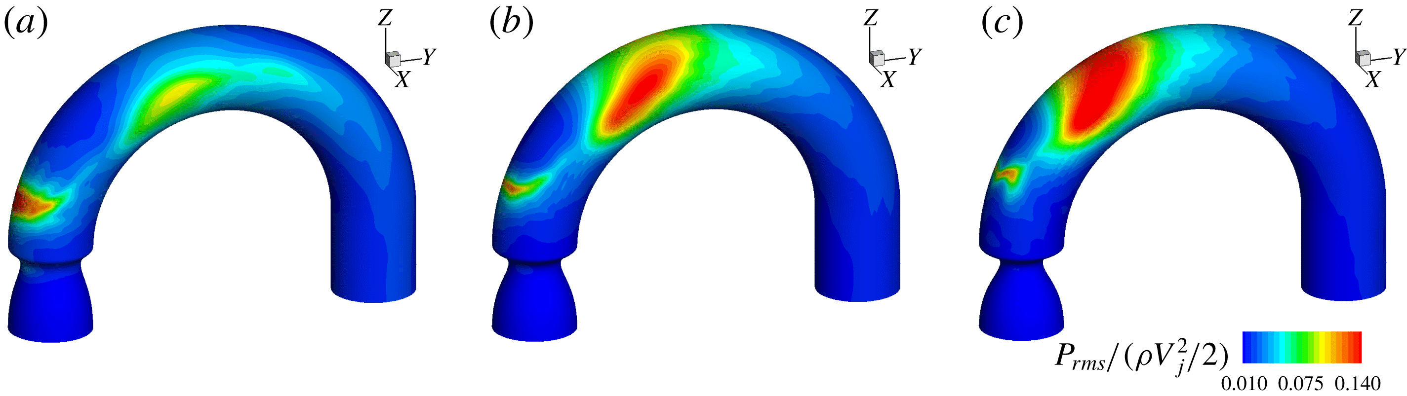
Non-dimensionalized RMS of surface pressure distribution for (a) $AS=50\,\%$ , (b) $AS=62.5\,\%$ and (c) $AS=75\,\%$ . All of the plots share the same contour levels as shown in (c).

Figure 12.

Non-dimensionalized RMS of WSS distribution for (a) $AS=50\,\%$ , (b) $AS=62.5\,\%$ and (c) $AS=75\,\%$ . All of the plots share the same contour levels as shown in (c).

Figures 11 and 12 plot the distribution of the RMS of wall pressure and WSS. The pressure fluctuations are expected to generate both compression (longitudinal) and shear (transverse) waves inside the thorax, while WSS fluctuations will primarily generate shear waves (Seo et al. Reference Seo, Bakhshaee, Garreau, Zhu, Andreou, Thompson and Mittal2017; Zhu et al. Reference Zhu, Seo, Bakhshaee and Mittal2017). Interestingly, the region in the vicinity of the stenosis and the location of jet impingement on the wall are correlated with low magnitude of pressure fluctuations as well as low WSS fluctuations. The strong surface force fluctuations are found to occur in the small recirculation region immediately after the stenosis as well as on the anterior and posterior surfaces of the ascending aorta. The surface force fluctuations on the anterior aortic lumen are of particular importance, since this surface faces the chest, where heart murmurs are typically detected.

It is readily noticed that the intensity of wall pressure fluctuation has very different distributions in this region for the three cases. For $AS=50\,\%$ , a single high-intensity region is observed on the anterior surface around $\unicode[STIX]{x1D703}=70^{\circ }$ . This location is well correlated with strong TKE cores in figure 10, which also occur in this general region. This TKE is mainly caused by the strong secondary flow and it is therefore reasonable to deduce that this strong wall pressure fluctuation is also related to the stochastic fluctuations inside the Dean vortices. On the other hand, the region of strong wall pressure fluctuations for $AS=62.5\,\%,75\,\%$ spans a large area on the anterior (and posterior) wall of the modelled aorta. In the $AS=75\,\%$ case, the anterior and posterior regions of high wall pressure fluctuation are joined together to form a single region that spans a large portion of the aortic arch. This behaviour can also be traced back to the TKE distribution. First of all, from figure 10, the two ends of the TKE bridge lie very close to the anterior/posterior surface, and they show strong intensity over a wide angle ( $55^{\circ }\leqslant \unicode[STIX]{x1D703}\leqslant 75^{\circ }$ ). This causes the large hotspot on the anterior surface. Second, the breakup of the jet shear layer occurs closer to the outer wall as the severity of the stenosis increases, which also introduces significant pressure fluctuations near the outer wall in the last two cases. It is readily noticed that the TKE reaches its maximum around $65^{\circ }$ for the last two cases, and this explains why the source location for the $AS=50\,\%$ case appears to be further downstream.

Figure 13.

(a) Non-dimensionalized RMS of pressure and (b) non-dimensionalized RMS of WSS plotted along the anterior surface.

Unlike the RMS of wall pressure, the surface distribution of the WSS fluctuations is more consistent among the three cases. Apart from the hotspot caused by the small recirculation zone immediately after the stenosis (arrow $A$ in figure 3), the maximum intensity of WSS fluctuation is located on the anterior and posterior surfaces of the ascending aorta, and is closely associated with the location of the Dean vortices. The RMS values of pressure and WSS are extracted along the anterior monitor points and plotted in figure 13. This figure clearly shows that the peak magnitude of the WSS fluctuation is approximately 5 % of that of the pressure fluctuation. Hence, the pressure fluctuation plays a dominant role in the murmur generation. From figure 13(a), the locations of the pressure fluctuation, i.e. the murmur source locations for $AS=50\,\%,62.5\,\%,75\,\%$ , are found to be at $\unicode[STIX]{x1D703}=70^{\circ },60^{\circ },55^{\circ }$ respectively. It is noted that even though the source locations span over $15^{\circ }$ , they actually lie within $0.6D$ of each other. This relative insensitivity of the murmur source to the stenotic severity is a reflection of the dominant role of the aortic curvature in the generation of pressure fluctuations.

3.5 Spectral analysis

One of the major motivations of this study is to correlate the characteristics of the murmurs, which are generated by the lumenal pressure fluctuations, with the degree of stenosis. Since the severity of the stenosis has a direct impact on the signal strength, researchers have previously examined the scaling of the maximum wall pressure fluctuation, with the intention of finding a universal scaling law that could relate the severity to the fluctuation intensity (Tobin & Chang Reference Tobin and Chang1976; Clark Reference Clark1977; Mittal et al. Reference Mittal, Simmons and Najjar2003). However, this is not an ideal metric in clinical practice since it requires careful calibration of the sensors and the measured signal strength is subject to various extraneous factors such as sensor contact condition, sensitivity and placement, as well as the thoracic anatomy of the patient. On the other hand, the frequency of the murmur signal can be measured with greater confidence as long as it is within the operating range of the sensor. In this section, we will focus on examining the frequency characteristics of the poststenotic flow in the modelled aorta.

Figure 14(a) shows the spectra corresponding to the streamwise velocity perturbation along the geometric centreline of the modelled aorta for the 75 % case. We can see that at the exit of the stenosis ( $\unicode[STIX]{x1D703}=0^{\circ }$ ), the flow is still laminar and has very low fluctuation intensity. As the jet propagates further downstream, the shear layer of the jet exhibits periodic vortex shedding, and the spectrum at $\unicode[STIX]{x1D703}=20^{\circ }$ shows a peak around $St=0.93$ . The reason why the peak is not very sharp is that the signal is collected in the core region of the jet instead of the shear layer. This shedding frequency is higher than that of the circular jet reported by other researchers. For instance, Beavers & Wilson (Reference Beavers and Wilson1970) studied the natural shedding frequency of the free circular jet and observed a shedding frequency of around 0.63 over a wide range of Reynolds numbers (500–3000). Similar numbers are also reported in other studies of a poststenotic jet in a confined straight tube (Johansen Reference Johansen1930; Cassanova & Giddens Reference Cassanova and Giddens1978; Ahmed & Giddens Reference Ahmed and Giddens1983b ). The reason for a similar shedding frequency for both free and confined circular jets is that these poststenotic flows are still dominated by the dynamics of the jet. The shear layer surrounding the core of the jet is less affected by the wall immediately after the stenosis, and its stability is still governed by the intrinsic mechanism of the shear layer instability. However, in the current study, even though the jet still maintains a circular shape right after the stenosis, the outer part of the jet impinges the outer wall before the shedding behaviour occurs. The resulting shear layer no longer maintains a circular shape and, hence, the characteristic shedding frequencies from straight tubes are not expected to predict the shedding frequency in this case.

Figure 14.

(a) Spectra corresponding to the temporal variation of the velocity plotted at selected $\unicode[STIX]{x1D703}$ along the centreline for $AS=75\,\%$ . The vertical line denotes $St=0.93$ . (b) Spectra corresponding to the temporal variation of the velocity plotted at selected $\unicode[STIX]{x1D703}$ for all three severities. Two turbulent scalings are also plotted to facilitate comparison. Here, $E_{k}$ and $St$ are defined as $\langle u_{i}^{\prime }u_{i}^{\prime }\rangle /V_{j}^{2}$ and $fD_{j}/V_{j}$ respectively.

Beyond the angle of $40^{\circ }$ , the discrete shedding frequency is no longer visible in the spectrum, and the flow starts to transition to turbulence. At $75^{\circ }$ , the spectrum corresponding to the velocity fluctuation clearly demonstrates turbulent flow scaling, as shown in figure 14(b). Two other spectra, corresponding to the signals at different locations of the $50\,\%$ and $62.5\,\%$ cases, are also plotted in figure 14(b). Both of them show reasonable agreement with the classic scalings (Tennekes & Lumley Reference Tennekes and Lumley1972; Hinze Reference Hinze1975), verifying the existence of turbulence in such flows. It is worth emphasizing that the signals plotted here are collected along the geometric centreline of the aorta. However, it is clearly shown in figure 10 that the locations selected here are not necessarily where turbulence develops first or is the strongest. This can also potentially explain the imperfect scaling of the 50 % case in the high-frequency range, since the TKE shows low intensity along the centreline there.

Figure 15.

The temporal variation of the non-dimensionalized pressure fluctuation at $\unicode[STIX]{x1D703}=35^{\circ }$ for $AS=75\,\%$ . The $y$ -axis is set to $[-0.2,0.2]$ to facilitate comparison.

Figure 16.

Spectra of the pressure fluctuation plotted at selected $\unicode[STIX]{x1D703}$ along the centreline for (a) the $75\,\%$ case and (b) all three cases. The vertical line denotes $St=0.93$ . Here, $E_{p}$ and $St$ are defined as $\langle p^{\prime }\rangle /(\unicode[STIX]{x1D70C}V_{j}^{2})/2$ and $fD_{j}/V_{j}$ respectively.

Pressure is of great interest in this study as it is responsible for the generation of the murmurs. In the following discussion, we will first explain the results for 75 % stenosis in detail, and then present the results from the other two cases in comparison with the 75 % case. Figure 15 shows the temporal history of the pressure fluctuations at $\unicode[STIX]{x1D703}=35^{\circ }$ for $75\,\%$ stenosis. Even though no clear periodicity can be observed in the signal from the centreline, it will be shown later that periodic vortex shedding is occurring at this location. Figure 16(a) illustrates how the spectrum of the pressure fluctuation evolves along the centreline. The flow is relatively quiescent coming out of the stenosis, and weak pressure fluctuations are observed at $\unicode[STIX]{x1D703}=0^{\circ }$ . As the jet propagates downstream, the shear layer becomes unsteady and discrete-frequency vortex shedding with a Strouhal number of 0.93 appears, as shown by the spectrum at $\unicode[STIX]{x1D703}=20^{\circ }$ . This characteristic frequency is consistent with the value obtained previously from the velocity spectrum. A clear peak at $St=0.93$ can be observed in the pressure spectrum from $20^{\circ }$ to $35^{\circ }$ , indicating a region where the vortex shedding is dominant. As the flow moves downstream, it transitions to turbulence and the aforementioned peak is no longer visible. The spectra of the centreline pressure fluctuation for the 50 % and 62.5 % cases demonstrate similar spatial evolution. In particular, the discrete vortex shedding frequency, when non-dimensionalized by the jet diameter and jet velocity, is around 0.93 for all three cases, as shown in figure 16(b). This specific frequency can be observed from $20^{\circ }$ to $55^{\circ }$ for $AS=50\,\%$ , and from $25^{\circ }$ to $40^{\circ }$ for $AS=62.5\,\%$ . It is noted that the vortex shedding develops around the same angle for all three cases. However, as the jet intensity increases with the severity of the stenosis, the location of the transition to turbulence moves upstream, leading to an early disappearance of the corresponding peak in the spectrum. Nevertheless, as will be shown later, the absence of this peak does not indicate a lack of contribution from the periodic vortex shedding to the flow in this region.

Figure 17.

(a) Spectra of the pressure fluctuation plotted at selected $\unicode[STIX]{x1D703}$ along the anterior surface for $AS=75\,\%$ . (b) Replot of the spectrum of the pressure fluctuation at $\unicode[STIX]{x1D703}=40^{\circ }$ along with a linear curve fitting whose details can be found in table 1. The vertical line denotes $St=0.93$ .

The surface pressure fluctuations are directly relevant to the generation of murmurs, and, in figure 17(a), we plot the spectra of the pressure fluctuation on the anterior surface at the same angles as in figure 16(a). It is immediately apparent that there is no clear peak at $\unicode[STIX]{x1D703}=20^{\circ }$ , but, interestingly, the slope of the spectra at $\unicode[STIX]{x1D703}=40^{\circ }$ seems to change significantly across $St=0.93$ . This change of slope has been observed in previous experimental (Tobin & Chang Reference Tobin and Chang1976) and numerical (Seo & Mittal Reference Seo and Mittal2012) studies. The frequency at which the slope changes, usually called the ‘break frequency’ or ‘corner frequency’, has been identified as an important metric in electronic auscultation-based determination of the degree of stenosis (Duncan et al. Reference Duncan, Gruber, Dewey, Myers and Lees1975).

Using a piecewise linear regression, we have obtained the best fit lines of each side of the observed break frequency, $\tilde{f}_{bc}$ , as shown in figure 17(b). Here, the intersection of these two linear regressions gives the break frequency ( $f_{bc}$ ), and the difference between $f_{bc}$ and $\tilde{f}_{bc}$ indicates the quality of the approximation. From table 1, we can see that, for figure 17(b), the observed break frequency, which is also the shedding frequency of the shear layer, is sufficiently close to $f_{bc}$ . This means that even though no distinct peak from vortex shedding is present in the spectrum, the break frequency shows a significant contribution from the discrete vortex shedding to the pressure fluctuation.

Table 1.

Details of the least-squares-based linear curve fitting. Here, $\tilde{f}_{bc}$ is the observed break frequency and $f_{bc}$ is the break frequency calculated from the linear regression.

Figure 18.

Spectra of the pressure fluctuation at the source locations identified in figure 13(a) plotted with the corresponding linear curve fittings. Details of the linear curve fittings are provided in table 1. The vertical line denotes $St=0.93$ .

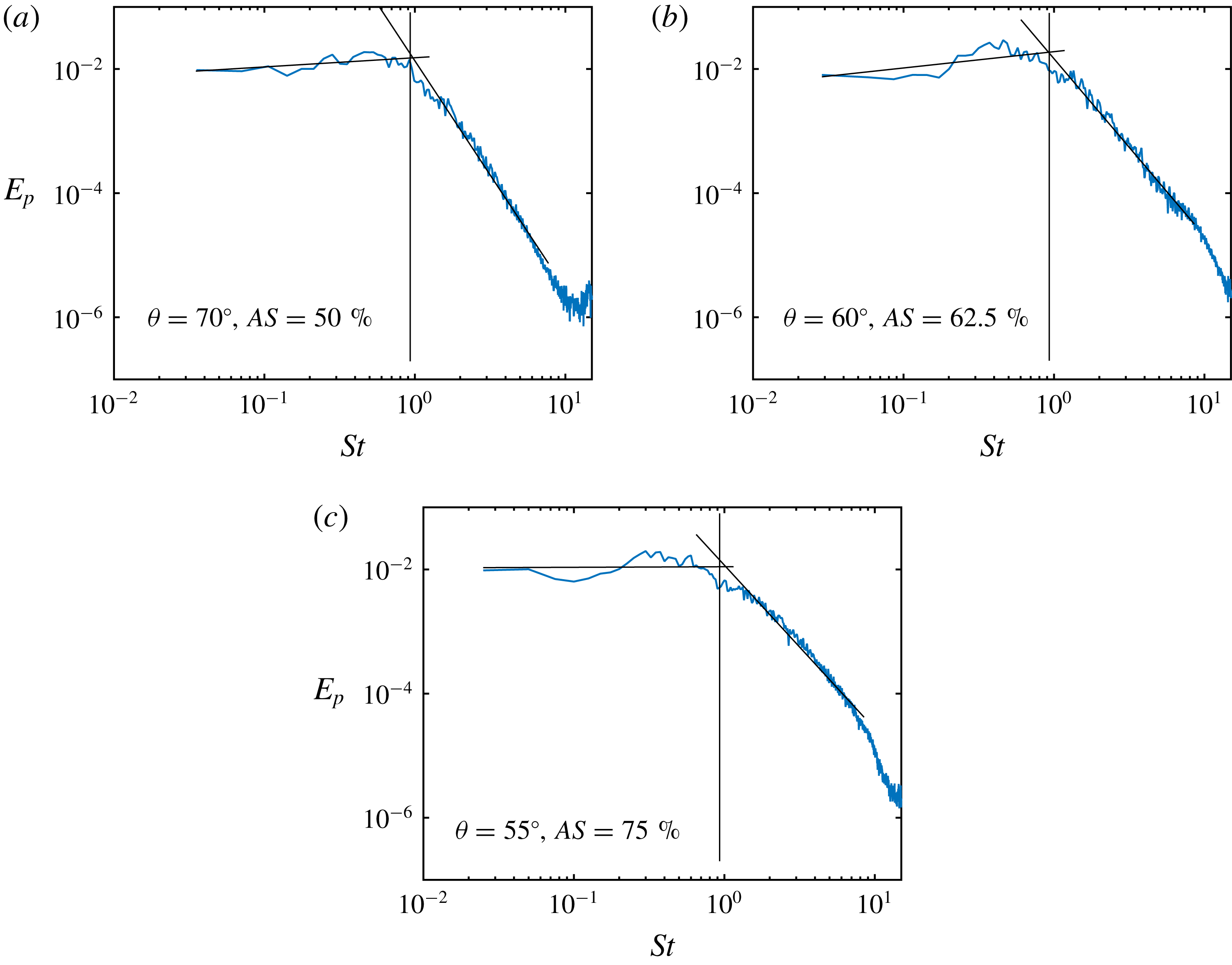
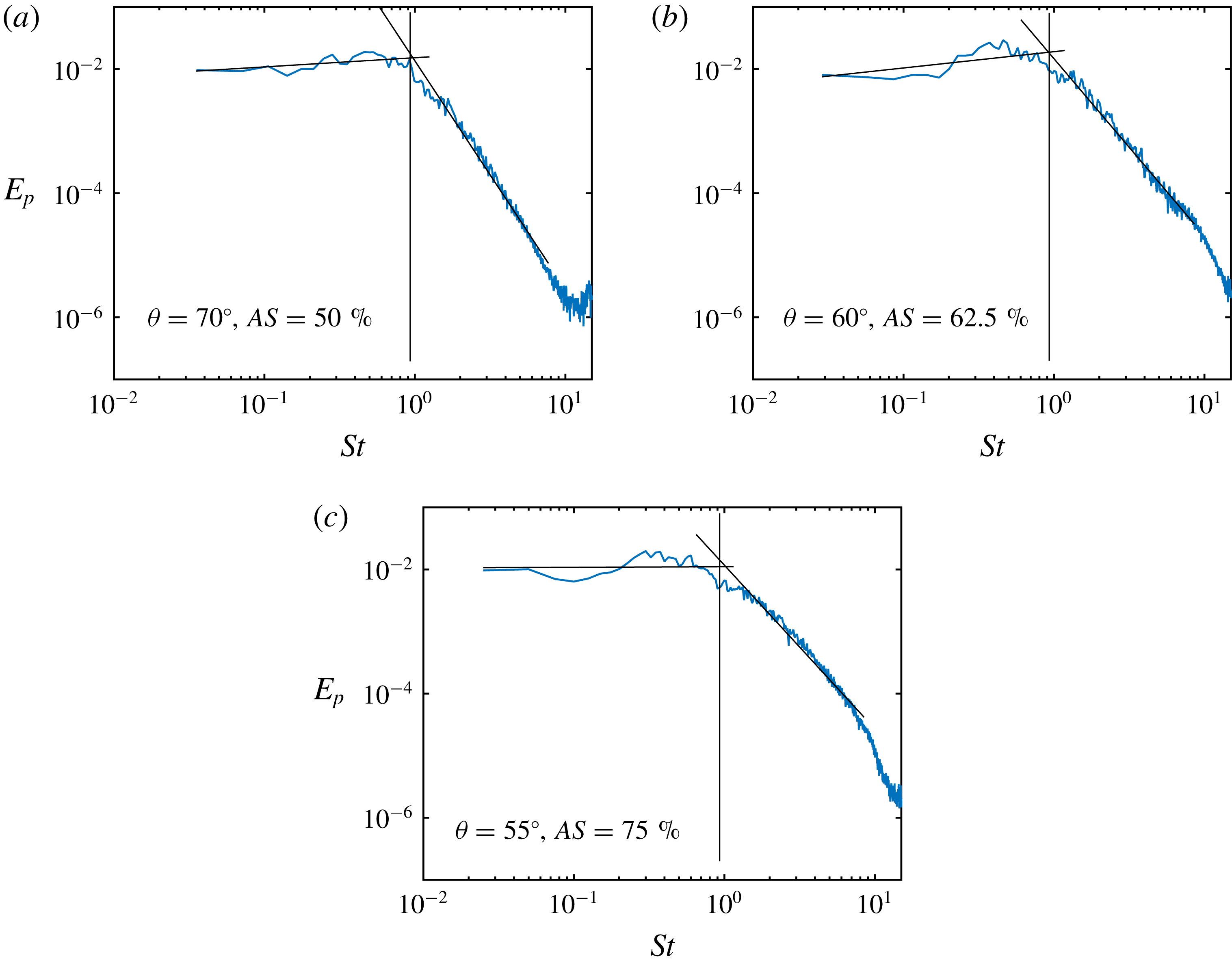
It is also useful to study the break frequency in the surface region identified as the primary source for the murmurs. Figures 18(a)–18(c) plot the spectra of pressure fluctuation at the source locations identified in figure 13(a) along with the linear curve fit, and $f_{bc}$ are determined to be sufficiently close to 0.93 for $AS=50\,\%$ and $62.5\,\%$ , indicating the significant contribution from the shear layer vortex shedding. On the other hand, $f_{bc}$ deviates slightly but noticeably away from this frequency for $AS=75\,\%$ , and this could be due to several reasons. First of all, the smaller jet size means that the vortex shedding occurs closer to the geometric centreline of the modelled aorta, and away from the anterior surface, making the frequency harder to transmit to the surface. Moreover, the strong jet is also likely to induce stronger turbulence, and increase the relative contribution of stochastic turbulent fluctuation to the wall pressure fluctuation.

Combination of the results in table 1 and figure 10 provides additional insight into the mechanism for murmur generation. Previous analysis shows that the location of strong wall pressure fluctuations is spatially well correlated with the location of intense turbulent fluctuations. However, the study of break frequency reveals that the total pressure fluctuations also contain contributions from the shear layer vortex shedding from upstream. In clinical practice, a 75 % area reduction is at the threshold between a mild and a severe stenosis. Severe stenosis causes noticeable symptoms in the patient and is therefore easy to detect. Mild stenosis, on the other hand, is asymptomatic and thus harder to detect. The spectral analysis shows that, for mild stenosis, the discrete-frequency shear layer shedding frequency is also the break frequency of the murmur source, and can potentially be sensed on the epidermal surface. Thus, auscultation may be a promising tool for detection and screening of early-stage aortic stenosis.