1. Introduction
Are the banking system and its regulatory framework prepared for the transition to a low-carbon economy? The commitment of global leaders to reduce carbon emissions following the Paris agreementFootnote 1 necessitates significant and abrupt changes in production activities, which could have adverse consequences for the banking sector. Transition risk shocks—such as carbon taxes or other policy measures to reduce carbon emissions—may be exacerbated by demand shocks as consumer habits and preferences evolve.Footnote 2 Additionally, these shocks may lead to increased corporate default correlations and overlapping portfolios,Footnote 3 potentially posing a material risk to the banking system.
Despite growing attention to climate risks, banks’ exposure to assets vulnerable to transition risk has seen little change in recent years. While emission intensity of banks’ portfolios has declined in key euro area countries, this was largely due to sectoral reallocations rather than reductions in the emissions of their exposures (see left panel of Figure 1). Meanwhile, industry breakdowns reveal that exposures to transition risk-prone sectors remain important (right panel of Figure 1).
Average emission intensity of banks’ exposures and exposures to different sectors of the economy.
Sources: Eurostat (emission intensity per sector), ECB, and ECB data calculations (sectoral exposures).
Notes: The bank sample includes the 167 largest euro area banks. The aggregation by country is done according to the country of the ultimate parent of each bank. The countries shown are (from left to right) Germany, Spain, France, Italy, and the Netherlands; “EA” represents the overall sample average. The emission intensity is measured as the ratio between greenhouse gas emissions (CO2, N2O in CO2 equivalent, CH2 in CO2 equivalent, HFC in CO2 equivalent, PFC in CO2 equivalent, SF6 in CO2 equivalent, and NF3 in CO2 equivalent) and the value added. The left panel shows the weighted average emission intensity of banks’ loan portfolio. Exposures are computed using as the share of credit exposures to firms in each sector of the economy over the total loan book. Weights are given by the emission intensity. The chart reports the average emission intensity of the exposures for 2015Q4 (blue bars), the average emission intensity of 2022Q4 exposures using the 2015Q4 emission intensity weights (yellow bars), and emission intensity of the exposures for 2022Q4 (red bars). The difference between the yellow and blue bars shows the impact of the exposure changes, and the difference between the yellow and red bars shows the impact of the emission intensity change.

The growing body of evidence highlighting the significance of climate-related risks for financial stability has ignited a debate on whether the current regulatory framework is sufficient to address both transition and physical risks.Footnote 4 These risks could potentially affect the safety and soundness of individual banks and the stability of the banking system as a whole.Footnote 5 Regulators and policymakers have been exploring various policy options to close potential regulatory gaps. These options range from enhanced disclosure requirements to microprudential capital requirements and macroprudential buffers.Footnote 6 Focusing on transition risk, we contribute to this ongoing debate by presenting theoretical evidence that supports the explicit incorporation of risks associated with the transition to a low-carbon economy into banking capital requirements. Our analysis compares the equilibrium outcomes of two models that are identical in all respects except for the way banks process information on transition risk.Footnote 7 In the first model, the absence of climate-related requirements leads banks to treat all firms identically with respect to transition risk. In the second model, climate-related prudential policies are introduced, requiring banks to assign different risk weights to firms according to their carbon emission intensity.
Our paper contributes to the literature assessing the impact of climate-related prudential regulation on the financial system (Carattini et al. (Reference Carattini, Heutel and Melkadze2023); Diluiso et al. (Reference Annicchiarico, Carli and Diluiso2023); Dunz et al. (Reference Dunz, Naqvi and Monasterolo2021); Oehmke and Opp (Reference Oehmke and Opp2022), among others). Differently from most of the literature, we focus explicitly on the need of prudential policies to address climate transition risks by justifying their application solely from a prudential and financial stability perspective and not assuming an additional ‘climate mitigation mandate’ of the prudential authorities. In the theoretical literature, this result is usually taken as given, and the objective of the papers is rather focused on studying the impact of different types of climate-prudential regulations on climate-related risks, the real economy and the financial sector or the climate itself (pollution and emissions).
The two models we compare are based on a dynamic stochastic general equilibrium (DSGE) framework and are used to investigate the efficiency of portfolio allocation in terms of banking sector risk-taking in the presence of transition risk. The model economy—identical in both models—includes households, banks, heterogeneous firms, a tax authority, a monetary policy authority, and a prudential authority. Banks finance two types of firms that differ in their emission intensity of their produced goods. Producing low-carbon-intensive products requires more expensive capital investments, whereas producing high-carbon-intensive goods is subject to emission taxes. Both types of firms are subject to standard idiosyncratic shocks driving credit risk (as in the literature starting from Bernanke et al. (Reference Bernanke, Gertler and Gilchrist1999)) which implies that they may default on their loans if their returns are insufficient to repay the bank. Banks aim to maximize their profits by optimally allocating their loan portfolios, subject to risk-sensitive capital requirements.
We make two key assumptions. First, we assume that transition risk is not the primary source of credit risk. In our models, transition risk arises from potential future additional taxes or regulations on emissions, which are uncertain at the current juncture. In practice, we reflect these factors in the two models by introducing a shock to emission taxes and a shock to the riskiness of carbon-intensive entrepreneurs, which increases their likelihood to default in equilibrium. However, these taxes are unlikely to rise to very high levels due to the significant costs they would impose on consumers and firms. Second, we assume that banks have low incentives to internalize transition risks. Identifying credit risk driven by transition risk would imply additional costs for banks, such as investments in databases, re-estimating or developing new credit risk models, and recruiting specialized staff. Coupled with the uncertainty of transition risk, these additional costs further disincentivize banks from properly accounting for such risks in their portfolios. For this reason, without policy intervention, banks do not distinguish between borrowers with different degree of carbon intensity.
As banks in our model without climate policy lack sufficient incentives to differentiate the transition risk associated with various credit exposures, credit contracts reflect the average level of risk across all firms. Consequently, the credit risk of high-carbon-intensive firms is underestimated (as they are characterized by higher-than-average transition risk) and overestimated for greener firms. Given that capital requirements are a non-linear function of credit risk, banks fail to hold enough capital to adequately cover transition risk and thus become over-invested in high-carbon-intensive firms.
In our assessment, we focus on comparing the equilibrium outcomes of the two models: with and without climate-prudential policy intervention. Specifically, we examine the allocation of the credit portfolio and the resulting credit volatility in the presence of transition risk shocks to determine if policy intervention can yield a superior outcome. We make two key modeling assumptions regarding the policy intervention. First, we abstract from specifying a precise climate-prudential policy instrument, assuming instead that the policy provides sufficient incentives for banks to fully internalize transition risk in their credit risk assessment. This could be achieved in practice through measures like transparency requirement or differentiated risk weights across sectors (like add-ons or supporting factors). Second, we assume that the requirements for more carbon-intensive exposures are relaxed when transition risk materializes. This means that we consider climate-prudential policies that increase the banking system’s resilience to transition shocks, rather than reducing the likelihood of these shocks occurring. We model this by applying a lower risk weight to these exposures when the transition shock occurs. This assumption is common in the recent literature on the costs and benefits of prudential policies (see for example Budnik et al. Reference Budnik, Dimitrov, Giglio, Groß, Lampe, Sarychev, Tarbe, Vagliano and Volk2021) and aligns with current policy practices. We have observed both microprudential and macroprudential policies being relaxed in response to shocks.Footnote 8
By comparing the outcome of these two models—with and without climate-prudential policy intervention—we find that if banks were to fully internalize transition risk, they would reduce their exposure to high-carbon-intensive firms. This suggests that, in the absence of prudential policies, banks engage in excessive risk-taking, and aggregate capital requirements are insufficient to cover all credit risk. Consequently, this leads to excessive risk-taking and increased lending volatility relative to the case where banks are required to internalize firm-specific transition risk. Moreover, in the absence of climate-prudential regulation, low-carbon-intensive firms are charged higher interest rates that partially pay for the transition risk associated with high-carbon-intensive firms, while the latter benefit from relatively lower rates. This inequitable risk-pricing is what ultimately steers portfolio allocations toward high-carbon-intensive firms, thereby encouraging greater risk-taking by banks. We further show that climate-prudential policies, which require banks to set capital requirements that distinguish between the two types of firms, reduce credit and output volatility. Consequently, a prudential framework including such policies is Pareto superior to a framework that lacks such measures. This result is significant as it is the first in the literature to highlight the need for regulation that addresses transition risks purely based on financial stability arguments. Moreover, these policies would benefit the monetary policy authority by enabling a more effective stabilization of the real economy.
The rest of the paper is organized as follows: Section 2 provides an overview of the relevant literature. In Section 3, the general structure of the two models—with and without climate-prudential policies—is presented. We discuss our results in Section 4, whereas Section 5 presents the robustness of our results. Conclusions are presented in Section 6.
2. Literature
Our paper contributes to a small but growing literature assessing the relevance of financial regulation to address climate-related risks to the financial system.Footnote 9 This literature includes mainly theoretical models,Footnote 10 with a majority of macro-financial models developed recently.
In a micro-theoretical setting, Oehmke and Opp (Reference Oehmke and Opp2022) study the positive and normative implications of climate change for bank capital regulation under either a prudential mandate or a broader climate mandate. They find that climate-related risks that affect banks’ stability can be optimally addressed by a combination of green supporting and dirty penalizing factors.
A few papers have used different types of macro-financial models to analyze the impact of green regulatory policies on climate-related risks and financial stability. For example, Dafermos and Nikolaidi (Reference Dafermos and Nikolaidi2021) use an agent-based stock-flow-consistent model to study the impact of capital requirements that differentiate between loans to firms with different degrees of carbon emissions. In their setting, capital requirements are determined according to the ‘degree of dirtiness’ of the underlying investment, and the ‘dirty penalizing factor’ has a positive effect on financial stability only if applied jointly with climate-related fiscal policy. Also in a stock-flow consistent model, Dunz et al. (Reference Dunz, Naqvi and Monasterolo2021) study the impact of a carbon tax and of a green supporting factor on the banking sector’s performance and show that although investments with low carbon emissions are boosted in the short run, these policies might negatively impact financial stability. They further demonstrate that only if the government applies a redistributive welfare policy or if banks reallocated their portfolios towards low-carbon emission investments, financial stability and a smooth transition to a low-carbon economy are achieved. Moreover, in another agent-based model, Lamperti et al. (Reference Lamperti, Bosetti, Roventini, Tavoni and Treibich2021) study the impact of using zero risk weights for exposures to firms with low carbon emissions. The authors show that physical climate risks increase the probability of having a banking crisis, and only a policy mix combining capital requirements more favorable towards low-carbon emission exposures, public guarantees on credit to low-carbon exposures, and carbon-risk adjustment in credit ratings leads to a stable financial sector (and at the same time lower emissions and higher economic growth).
Punzi (Reference Punzi2019) represents an early attempt to analyze different regulatory policies in an Environmental-DSGE (E-DSGE) context, with a focus on how to increase financing to low-carbon-emission firms. Compared to our paper, her analysis imposes non-risk-based regulatory rules and considers each rule separately. In this setting, she finds that only differentiated capital requirements can encourage green financing. Also in an E-DSGE setting, Carattini et al. (Reference Carattini, Heutel and Melkadze2023) show that policies in the form of taxes or subsidies on banks’ assets can help to guard against transition risks. In a DSGE model with financial frictions and differentiated energy sectors, Diluiso et al. (Reference Diluiso, Annicchiarico, Kalkuhl and Minx2020) show that transition risk generated by an ambitious climate policy is limited and that green financial regulation via tax-subsidy schemes might increase financial instability. However, they find that unconventional monetary policy (green credit policy) in response to a financial crisis triggered by transition risk can stabilize the banking sector and at the same time encourage aggregate demand. Using a multi-sector DSGE model with default, Giovanardi and Kaldorf (Reference Giovanardi and Kaldorf2023) find only limited effects of using higher risk weights for brown assets as climate policy tool, whereas they find that differentiated risk weights can affect risk-taking and default rates of banks. In a E-DSGE model with bank default, Garcia Villegas and Martorell (Reference Garcia Villegas and Martorell2024) find that, in the presence of transition risk, increasing capital requirements for banks’ fossil exposures are welfare superior to a general increase in capital requirements. Finally, Diluiso et al. (Reference Annicchiarico, Carli and Diluiso2023) show that countercyclical capital requirements—taking the form of reserve requirements—can reduce the uncertainty surrounding the functioning of carbon-pricing policies throughout the business cycle, using a DSGE model with financial frictions.
Compared to the aforementioned literature, we explicitly show with our model that transition risk leading to higher riskiness of high-polluting firms can indeed have a negative impact on financial stability. This, in turn, would make the case for a policy intervention by the prudential authority. In the theoretical literature, this result is usually taken as givenFootnote 11 and the objective of the papers is rather focused on studying the impact of different climate-prudential regulations on (i) Climate-related risks, (ii) The real economy, (iii) The financial sector or (iv) The climate itself (pollution and emissions). Three papers have however also looked at the financial stability implications of transition risk (Carattini et al. Reference Carattini, Heutel and Melkadze2023; Diluiso et al. Reference Diluiso, Annicchiarico, Kalkuhl and Minx2020; Dunz et al. Reference Dunz, Naqvi and Monasterolo2021), but in a different manner than we do. Dunz et al. (Reference Dunz, Naqvi and Monasterolo2021) use a stock-flow consistent model, whereas we opt for a DSGE model with financial frictions and heterogeneous banks and firms. Carattini et al. (Reference Carattini, Heutel and Melkadze2023) show indeed that an ambitious climate (fiscal) policy can have implications for financial stability, but consider taxes and subsidies on banks’ assets as regulatory policy options, whereas in our model we analyze prudential regulation based on risk-weighted assets, in line with the Basel III framework.Footnote 12 Finally, Diluiso et al. (Reference Diluiso, Annicchiarico, Kalkuhl and Minx2020) use a DSGE model to show that transition risk arising from a credible medium-term emission reduction strategy has only a limited impact on banks’ net worth, thus not necessarily showing the need of prudential policy intervention to deal with this type of climate risk.
Modeling wise, our paper is based on the DSGE literature featuring a financial sector and financial frictions in the spirit of Bernanke et al. (Reference Bernanke, Gertler and Gilchrist1999) and all the literature that developed afterwards (for e.g. Gerali et al. (Reference Gerali, Neri, Sessa and Signoretti2010); Gertler and Karadi (Reference Gertler and Karadi2011); Gertler and Kiyotaki (Reference Gertler and Kiyotaki2010) and Darracq-Pariès et al. (Reference Darracq-Pariès, Kok and Rodriguez-Palenzuela2011), among many others). We build on the Darracq-Pariès et al. (Reference Darracq-Pariès, Kok and Rodriguez-Palenzuela2011) and Darracq-Pariès et al. (Reference Darracq-Pariès, Kok and Rancoita2019) models. However, instead of two firms producing either residential and non-residential goods, we introduce heterogeneous firms which differ in their degree of carbon emissions. As in the rest of the E-DSGE literature, we assume emissions are a (non-linear) function of production.
3. The Model
To assess the need for climate-related prudential regulation, we develop and compare two models that differ only in how banks process information into their risk assessment. In all other respects, the two models are identical. The two DSGE models include three main types of agents—households, heterogeneous firms, and banks. Households offer their labor services to the different firms in the economy, consume an aggregate basket of goods produced by firms, and save their money in the form of deposits. Firms that populate the economy produce differentiated goods and have different levels of carbon emissions. Less carbon-intensive firms use more technologically advanced (and expensive) capital in their production process which allows them to be less polluting than more carbon-intensive firms which use regular capital. Firms pay taxes depending on their carbon emissions which are the source of transition risk in the model. To finance their production, firms use in addition to their own net worth, funds coming from a bank. As firms are subject to idiosyncratic shocks, they might default on their loan commitment and cause losses to the bank (in the spirit of Bernanke et al. (Reference Bernanke, Gertler and Gilchrist1999); Darracq-Pariès et al. (Reference Darracq-Pariès, Kok and Rancoita2019); Gerali et al. (Reference Gerali, Neri, Sessa and Signoretti2010)). This asymmetric information between firms and banks implies that the entrepreneurs are financially constrained and that the interest rate (the external finance premium) established in the loan contract will depend on their leverage. The model includes also capital producers that provide differentiated capital to goods-producing firms and retailers which operate in monopolistic competition to insure sticky prices (Calvo Reference Calvo1983). A monetary policy authority sets the risk free rate, whereas the government collects taxes and transfers them to households.
Without loss of generality, we assume that the differences between firms’ credit risk arise only due to transition risk. Banks are operating in a perfectly competitive environment and collect deposits from households, provide funds to firms, and are subject to risk-sensitive capital requirements. In the case of a firm’s default, banks incur a monitoring cost which allows them to recover the collateral associated to the credit contract.
It is within the banking sector that the two models differ. In the first model—aligned with the Basel III framework but without any climate-prudential regulation—banks do not distinguish between firms based on their carbon emissions. They treat all firms identically, using aggregated firm-level data to estimate default probabilities and assign risk weights accordingly. In contrast, the second model introduces a supplementary regulatory constraint requiring banks to explicitly differentiate between firms with a high carbon intensity and those with low carbon emissions. As a result, banks compute separate default probabilities and apply differentiated risk weights to each category.
The core mechanism through which transition risk is transmitted in these models operates as follows: an increase in the carbon tax has a direct impact on production costs for polluting firms, reduces their profitability, and consequently increases their probability of default. Additionally, transition risk increases the uncertainty surrounding the production environment in which polluting firms operate (as it might imply more fundamental changes to the production environment), which further increases the riskiness of these firms. In the absence of climate-prudential regulation, banks apply an average default probability across all firms, regardless of carbon intensity. As a consequence, polluting firms benefit from more advantageous financing conditions than in the climate policy model, whereas low-carbon-intensive firms are penalized with overly restrictive credit conditions that do not reflect their lower risk. Moreover, in this model without climate regulatory requirements, banks may be inadequately capitalized when transition risk materializes. Conversely, if banks account for climate transition risk by explicitly distinguishing firms according to their carbon emissions (e.g., based on their ESG scores), they apply risk weights that reflect the exposure’s degree of carbon intensity. This would in turn lead to higher lending rates and reduced credit for polluting firms. Overall, the implementation of climate-related prudential regulation is expected to reduce banks’ exposure to transition risk by inducing a portfolio reallocation toward less risky firms, thereby enhancing financial stability.
We assume that climate-prudential policy enables a perfect identification of transition risks across firms (i.e., a first-best scenario). In practice, this could be implemented through instruments such as risk-weight adjustments (add-ons or supporting factors) or mandatory disclosure of transition risks associated with exposures. The policy would also ensure that capital requirements are relaxed for certain exposures as transition risks materialize, in line with existing prudential measures. This assumption is consistent with recent institutional literature emphasizing the role of prudential policies in enhancing banks’ loss-absorption capacity rather than directly preventing crises (see, for example, Budnik et al. Reference Budnik, Dimitrov, Giglio, Groß, Lampe, Sarychev, Tarbe, Vagliano and Volk2021). In practice, both microprudential and macroprudential requirements can be relaxed in response to shocks,Footnote 13 with prudential buffers calibrated to ensure sufficient loss-absorption capacity under adverse scenarios. Our modeling framework incorporates these features.
3.1. Households
Households supply labor to different types of firms which are characterized by different levels of carbon intensity (
 $L_t^i$
, where
 $i = \{HCI,LCI\}$
indicates the classification of firms by carbon emissions, high or low carbon intensity) for which they get paid an hourly wage (
 $w_t^i$
), consume a mixed basket of goods from all firms (
 $C_t^H$
), and save their income in the form of deposits
 $D_t$
which are remunerated at the risk-free rate
 $R_t$
. Households are also the owners of banks and of retail firms from which they receive dividends (
 $\Pi _t^H$
). In addition, they receive benefits
 $G_t$
from the government. They maximize their utility so as to choose consumption, hours worked, and deposits:
 \begin{eqnarray} \max _{\{C_t^{H,i},L_t^i,D_t^H\}} \mathbb{E}_{t}\left [\sum _{t=0}^{\infty } \beta ^{H^t} \left (\frac {C_{t}^{{H}^{1-\gamma }}}{1-\gamma } - \sum _i \overline {L}^i\frac {L_{t}^{i^{1+\sigma ^i}}}{1+\sigma ^i}\right )\right ] \end{eqnarray}
subject to the budget constraint expressed in nominal terms:
 \begin{eqnarray} \sum _i P_t^i C_t^{H,i}+P_t D_t^H \leq P_t \frac {1+R_{t-1}}{1+\pi _t}D_{t-1}^H + \sum _i w_t^i L_t^i + \Pi _t^H +G_t. \end{eqnarray}
where
 $\pi _t$
is the aggregate inflation rate and
 $P_t$
is the aggregate price index. The parameters
 $\overline {L}^i$
in the utility function are calibrated such that at the steady state total labor is normalized to one. Household consume a basket
 $C_t^H$
of goods produced by all firms and
 $C_t^{H,i}$
indicates the consumption of goods with a specific emission intensity. Overall, the households’ preferences across different types of goods follow a CES form:
 \begin{eqnarray} C_t^H &=& \left [ \sum _i \kappa ^{i^{\frac {1}{\varepsilon }}} C_t^{{H,i}^{\frac {\varepsilon -1}{\varepsilon }}} \right ]^{\frac {\varepsilon }{\varepsilon -1}}, \end{eqnarray}
where
 $\sum _i \kappa ^i = 1$
.
3.2. Entrepreneurs
Firms produce differentiated goods of the same product category (e.g. electric and gas cars), and they are classified according to their level of carbon emission (
 $i = \{HCI,$
 $LCI\}$
, high or low carbon intensity). This classification could include both the production and the product, similarly to the Scope 3 ESG score. Low-carbon-intensive (LCI) firms use more technologically advanced (and costly) capital than high-carbon-intensive (HCI) firms allowing them to produce either with less emissions or more environmentally friendly products. Firms have to pay taxes for their carbon emissions, which are the source of transition risk in the model. Without loss of generality, we suppose that firms have otherwise the same solvency profile (i.e., the same ‘traditional’ credit risk) and differ only in their production technology and emission costs. Entrepreneurs own the firms and use their earnings for consumption, maximizing the utility from the consumption of a basket of differentiated goods:
 \begin{eqnarray} \max _{\{C_t^{E,i,j},L_t^i,K_t^i,B_t^i,u_t^i,\overline {\omega }_t^i\}} \mathbb{E}_{t}\left [\sum _{t=0}^{\infty } \beta ^{E^t} \frac {C_t^{{E,i}^{1-\gamma }} }{1-\gamma } \right ], \end{eqnarray}
where
 $C_t^{E,i}$
is the basket of differentiated goods consumed by entrepreneurs of type
 $i$
. As for the households, the consumption of goods with different degree of carbon intensity follows CES preferences:
 \begin{eqnarray} C_t^{E,i} &=& \left [ \sum _j \theta ^{j^{\frac {1}{\varepsilon }}} C_t^{{E,i,j}^{\frac {\varepsilon -1}{\varepsilon }}} \right ]^{\frac {\varepsilon }{\varepsilon -1}}, \end{eqnarray}
with
 $j = \{HCI,$
 $LCI\}$
the type of good consumed by entrepreneur
 $i$
. The production function of each firm (
 $Z_t^i$
) is Cobb-Douglas:
 \begin{eqnarray} Z_t^i &=& \epsilon _t^i \left (u_t^i K_{t-1}^i\right )^a \left (L_t^i\right )^{1-a} \end{eqnarray}
where
 $u_t^i$
is the capacity utilization,
 $K_t^i$
is the capital, and
 $\epsilon _t^i$
is a technology shock following an AR(1) process. Each period, firms take loans
 $B_t^{E,i}$
from banks to finance their activities. The interest rate associate with the loan is
 $R_{t}^{E,i}$
. However, firms are subject to idiosyncratic shocks affecting their revenues,
 $\omega _t^i$
, causing the default of some firms on the loan contract. If a firm does not repay its loan, the bank can seize the collateral
 $(1-\delta )Q_t^i K_{t-1}^i$
, where
 $Q_t^i$
is the nominal price of capital and
 $\delta$
a depreciation factor (see Darracq-Pariès et al. (Reference Darracq-Pariès, Kok and Rodriguez-Palenzuela2011, Reference Darracq-Pariès, Kok and Rancoita2019); Gerali et al. (Reference Gerali, Neri, Sessa and Signoretti2010), among others). Calling
 $\overline {\omega }_t^i$
the idiosyncratic shock at which the entrepreneur is indifferent between defaulting or not, firms are willing to pay the interest rate implied by this threshold:
 \begin{eqnarray} \frac {1+R_{t-1}^{E,i}}{1+\pi _t}P_t B_{t-1}^{E,i} &=& \overline {\omega }_t^i(1-\delta )Q_t^i K_{t-1}^i. \end{eqnarray}
This also implies that the expected loan repayment can be written as (see Bernanke et al. Reference Bernanke, Gertler and Gilchrist1999):
 \begin{eqnarray} H(\overline {\omega }_t^i)(1-\delta )Q_t^i K_{t-1}^i &\equiv & (1-\delta )Q_t^i K_{t-1}^i \left [ \int _0^{\overline {\omega }_t^i} \omega dF(\omega ) + \left (1-F\left (\overline {\omega }_t^i\right )\right )\overline {\omega }_t^i\right ]. \end{eqnarray}
Firms use different capital in their production functions which they acquire from the capital goods producers. In line with previous literature, we assume that both types of firms face adjustment costs related to capacity utilization, which we model as
 $\Phi _i(u_t^i) = \phi ^i r^{i,SS} (\exp [\frac {1}{\phi ^i}(u_t^i - 1) ] - 1)$
. Smets and Wouters (Reference Smets and Wouters2007) found that adjustment costs are key to fit New Keynesian models with empirical data. Our adjustment cost function is based on Darracq-Pariès et al. (Reference Darracq-Pariès, Kok and Rodriguez-Palenzuela2011) and implies that the cost of capacity utilization is zero at the steady-state level of the utilization rate (
 $\Phi ^i(1) = 0$
), and increases non-linearly as utilization deviates from this level. Furthermore, we assume that the adjustment cost parameter is higher for LCI firms than for HCI firms (i.e.,
 $\phi ^{LCI} \gt \phi ^{HCI}$
),Footnote
14
reflecting the greater technological and operational constraints faced by cleaner production technologies. While HCI firms often rely on conventional technologies (e.g., fossil fuel-based production), which allow relatively easy and low-cost adjustments to capacity utilization, LCI firms tend to use cleaner but more rigid technologies. For example, in the electricity sector, traditional gas or coal power plants can ramp up or down production relatively quickly, incurring relatively small costs when adjusting utilization. In contrast, renewable energy sources like wind or solar power are subject to intermittency and external conditions (e.g., weather), limiting their ability to flexibly adjust production. Increasing the effective use of capital in such contexts often requires costly complementary investments (e.g., battery storage, grid integration, or hybrid systems).
Firms also differ because they are subject to emission taxes
 $T(e_t^i)$
on the basis of their carbon intensity. In addition, each firm sells its goods to retailers, who will then distribute them to households at a price
 $P_t^i$
charging a markup on the price at which they buy the intermediate goods from entrepreneurs. The inverse of the markup charged by retailers on the intermediate good price is indicated with
 $\mu _t^i$
. The budget constraint in nominal terms writes:
 \begin{eqnarray} &\sum _j P_t^j C_t^{E,i,j} + Q_t^i\left [K_t^i - (1-\delta )K_{t-1}^i \right ] + w_t^i L_t^i + \Phi _i(u_t^i)K_{t-1}^i \nonumber \\&\quad +\, H(\overline {\omega }_t^i)(1-\delta )Q_t^i K_{t-1}^i + T(e_t^i) \leq \mu _t^i P_t^i Z_t^i + P_t B_t^{E,i} \end{eqnarray}
where the tax on emissions is a linear function of production:
 \begin{align} T(e_t^i) &= \epsilon ^T_t\eta ^i e_t^i \end{align}
 \begin{align} e_t^i &= \zeta Z_t ^i. \end{align}
where the parameter
 $\eta ^i$
represents the tax level and where
 $\zeta$
is the fraction of emissions to output (Benmir and Roman Reference Benmir and Roman2020). In our framework, we model a transition risk shock as a shock to the emission tax, represented in Eq. (10) by the variable
 $\epsilon ^T_t$
. This shock is assumed to be correlated with a shock to the riskiness of high-carbon-intensive entrepreneurs,Footnote
15
to capture the broader effects of transition policy shocks that go beyond a simple linear rise in production costs. While the increase in costs alone would already raise default probabilities, this representation does not fully reflect the nature of transition risk. Some policies have far-reaching implications for certain sectors, including fundamental changes to the competitive environment, the need to adopt new production technologies, or exposure to future regulation.Footnote
16
In this sense, the correlation captures the increased uncertainty surrounding the production environment in which HCI firms operate following the announcement or implementation of transition measures.”
Firms in each sector are in perfect competition in producing their goods; this implies the following zero-profit condition on production:
 \begin{eqnarray} \mu _t^i P_t^i Z_t^i - T(e_t^i) &=& \Phi _i'(u_t^i)u_t^i K_{t-1}^i + w_t^i L_t^i \end{eqnarray}
When maximizing their utility, firms also take into account the participation constraint of commercial banks to the lending contract. Commercial banks have financing costs
 $R_t^{F,i}$
for their loan contract and face some monitoring costs,
 $\rho$
to collect the collateral in case of default. Their participation constraint can be written as:
 \begin{eqnarray} \frac {1+R_{t-1}^{F,i}}{1+\pi _t}P_t B_{t-1}^{E,i} &\leq & (1-\delta )Q_t^i K_{t-1}^i G(\overline {\omega }_t^i) \end{eqnarray}
where:
 \begin{eqnarray} G(\overline {\omega }_t^i) & \equiv & \bigg [ (1-\rho ) \int _0^{\overline {\omega }_t^i} \omega dF(\omega ) + (1-F(\overline {\omega }_t^i))\overline {\omega }_t^i\bigg ]. \end{eqnarray}
3.3. Capital goods producers
There is a capital goods producer for each type of firm, HCI and LCI. Capital goods producers operate under perfect competition and are owned by households. At the beginning of each period, they purchase the undepreciated capital
 $(1-\delta )K_{t-1}^i$
from entrepreneurs at real prices. Then they augment the capital stock using distributed goods and facing adjustment costs proportional to the investment,
 $I_t^i$
. The augmented capital stocks are sold back to entrepreneurs at the same prices at the end of the period. The maximization problem of capital producers can be written as:
 \begin{eqnarray} \max _{\{K_t^i,I_t^i\}} \mathbb{E}_{t}\left \{\sum _{t=0}^{\infty } \beta ^{H^t} \Big [ Q_t^i\left [ K_t^i - (1-\delta )K_{t-1}^i \right ] - I_t^i \Big ] \right \}\!, \end{eqnarray}
subject to the law of motion of capital:
 \begin{eqnarray} K_t^i = (1-\delta )K_{t-1}^i + \left [1-S\left (\frac {I_t^i}{I_{t-1}^i}\right )\right ]I_t^i, \end{eqnarray}
where
 $S(.)$
is the adjustment cost function defined as
 $S(x) = s0.5(x-1)^2$
and
 $s$
is a parameter and where
 $x= \tfrac {I_t}{I_{t-1}}$
is the gross rate of change in investment. Following standard practice in the DSGE literature (e.g. Christiano et al. Reference Christiano, Eichenbaum and Evans2005; Smets and Wouters Reference Smets and Wouters2007), we assume that capital goods producers face convex investment adjustment costs.Footnote
17
This functional form ensures that adjustment costs are zero at steady state (
 $S(1) = 0$
, no costs when investment is stable) and increase with the magnitude of investment changes, whether positive or negative. The economic rationale is that rapid increases in investment may require urgent reallocation of resources, while sharp reductions can lead to inefficiencies such as underutilized capacity or cancelation costs.
3.4. Retailers
Retailers are in monopolistic competition. They buy homogeneous intermediate goods
 $Z_t^i(j)$
at price
 $\mu _t^i P_t^i$
from the entrepreneurs; they differentiate the products and sell them to households and entrepreneurs. As aforementioned,
 $\mu _t^i$
represents the inverse of the gross markup of retail goods over intermediate goods, or otherwise stated the selling price of intermediate products. Retailers set their prices on a staggered basis à la Calvo (Reference Calvo1983): in each period only a fraction
 $1- \chi$
of retailers is able to re-optimize its nominal prices (
 $P_t^i(j)=\tilde {P}_t^i(j))$
, where
 $\tilde {P}_t^i(j)$
is the optimal price for retailer
 $j$
, while the remaining fraction
 $\chi$
cannot re-optimize and will set the prices as in the previous period (
 $P_t^i(j)=P_{t-1}^i(j)$
). The aggregate price dynamics is given by a weighted average of prices set by firms that re-optimize and prices from the previous period kept constant by non-reoptimizing firms:
 \begin{eqnarray} P^i_t=\left [\chi {P_{t-1}^i}^{1-\epsilon } + (1-\chi ) \tilde {P}_t^i(j)^{1-\epsilon }\right ]^{\frac {1}{1-\epsilon }} \end{eqnarray}
In aggregate, the production and price index functions of retailers follow a CES functional form:
 \begin{align} Y_t^i &= \left [ \int _0^1 Y_t^i(j)^{\frac {\epsilon -1}{\epsilon }}dj \right ]^{\frac {\epsilon }{\epsilon -1}} \end{align}
 \begin{align} P_t^i &= \left [ \int _0^1 P_t^i(j)^{1-\epsilon }dj \right ]^{\frac {1}{1-\epsilon }} \end{align}
which imply the following demand of intermediate goods of the individual retailer:
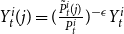 $Y_t^i(j) = ( \frac {\tilde {P}_t^i(j)}{P_t^i} )^{-\epsilon }Y_t^i$
. Then, each retailer who can re-optimize at
 $t$
maximizes the expected discounted stream of profits under the assumption that once the price
 $\tilde {P}_t^i(j)$
is set, he will not re-optimize with probability
 $\chi$
for a number of periods
 $k\in [0,\infty ]$
. The maximization of the retailer writes:
 \begin{eqnarray} \max _{\{\tilde {P}_t^i(j)\}} \sum _{k=0}^{\infty } \chi ^k \mathbb{E}_t \left [\lambda _{t+k}^{r,i}\left (P_{t+k}^i(j)- \mu _{t+k}^i P_{t+k}^i \right )Y_{t+k}^i(j)\right ] \end{eqnarray}
where
 $P_{t+k}^i(j)=\tilde {P}_t^i(j)$
for the assumptions above that the retailer will not re-optimize until
 $t+k$
.
3.5. Market clearing conditions for goods
For all goods, the aggregate demand and production are given by:
 \begin{align} Y_t^i &= C_t^{H,i} + \sum _j C_t^{E,j,i} + I_t^i + \Phi _B(u_t^i)K_{t-1}^i + \eta ^i\zeta Z_t^i \end{align}
 \begin{align} Z_t^i &= \varepsilon ^i\left ( u^i K_{t-1}^i\right )^a\left ( L^i_t\right )^{(1-a)} \end{align}
The market clearing condition in each good markets leads to the following relations:
 \begin{eqnarray} Z_t^i &=& \Delta ^i_t Y_t^i, \end{eqnarray}
where
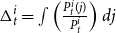 $\Delta _t^i = \int \left ( \frac {P_t^i(j)}{P_t^i}\right )dj$
measures the price dispersion among retailers.
3.6. The banking sector
The banking sector is modeled following Gerali et al. (Reference Gerali, Neri, Sessa and Signoretti2010) and Darracq-Pariès et al. (Reference Darracq-Pariès, Kok and Rodriguez-Palenzuela2011). As in this literature, we represent the banking system as composed of multiple specialized branches within a banking group, each with distinct role, as detailed below. This approach facilitates both the exposition and the mathematical tractability of the model.Footnote
18
In our framework, each banking group is composed of two branches that operate in a perfectly competitive environment. The wholesale branch receives deposits from households and allocates these funds to the commercial lending branch. The wholesale branch of the group also manages the capital position of the bank taking into account risk-sensitive capital requirements, and incurs a cost whenever the capital to risk-weighted assets ratio deviates from a target value,
 $CR$
. The commercial lending branch obtains funds from the wholesale branch and uses them to give credits to firms.
As shown in Section 3.2, taxes on carbon emissions affect credit risk increasingly with the level of carbon emission as they represent an additional cost. As the idiosyncratic shock
 $\omega ^i$
has the same distribution across types of firms, transition risk (i.e., the risk due to taxes on emissions) is the main source of differentiation of credit risk in the model. It is reasonable to assume that proportionally, credit risk due to transition risk is not more impactful than the more traditional source of credit risk as emission taxes cannot be raised abruptly to very high levels owing to the high costs this would impose on firms.
Internalizing the difference in credit risk of firms due to transition risk is costly for banks as this risk is quite challenging to identify and it would imply a number of additional costs for banks, such as investment in databases, the re-estimation or development of new credit risk models or the recruitment of specialized staff. Furthermore, part of the information would potentially not even be available or sufficient considering the short history of emission taxes or emission measurements.Footnote
19
As mentioned earlier, we compare two different specifications of the model which differ mainly in the modeling of the banking sector. The first specification of the model abstracts from any climate-prudential policy, while the second specification assumes that these policies are implemented. In our first model specification (without climate-prudential policies), banks have no incentive to internalize credit risk due to carbon taxes, i.e., transition risk, and therefore they do not distinguish between the degree of carbon intensity when lending. Thus, the estimation of the model is performed as if there was a single type of firm (indicated by
 $E$
) in the economy. Banks estimate their models based on aggregate data (for example, on capital investments), which is the weighted average of data from all firms. At the same time, entrepreneurs assume that banks can easily identify the carbon intensity of firms and therefore believe that banks provide individualized contracts. In terms of modeling, this implies that the participation constraint of commercial banks in the lending contract (eq. 13) remains as presented in Subsection 3.2, i.e., the participation constraint is specific to the type of firm.
In our second model specification, we assume that climate-prudential policies are implemented and banks have full incentives to identify the degree of firms’ carbon intensity and provide individualized contracts. In the next sections, we will describe each branch of the banking group.
3.6.1. The wholesale branch
We first present the wholesale branch for the model without climate-prudential policies before outlining the changes that are made to the model when we assume that banks have to identify firms on the basis of their carbon intensity. The wholesale branches receive deposits from households and choose the allocations of loans. The wholesale branches maximize their profits, taking interest rates as given and taking into account a penalty if the risk-weighted capital ratio deviates from a target capital ratio. Their profit maximization writes:
 \begin{eqnarray} \max _{\{B_{t}^{E}, D^{H}_t\}} R_{t}^{F,E}B_{t}^{E} - R_t D^{H}_{t} - PD_t^E LGD^E B^{E}_{t} - \frac {\Xi }{2} \left (\frac {Bankcap_t}{rw_t^E B_{t}^{E}} - CR\right )^2 Bankcap_t \end{eqnarray}
which is subject to the balance sheet identity:
 \begin{eqnarray} B_{t}^{E}=D^{H}_t+Bankcap_t \end{eqnarray}
where
 $D^H_t$
represents households’ deposits which are remunerated at the risk-free rate
 $R_t$
.
 $R_t^{F,E}$
represents the interest rate at which the wholesale branch gives funds to its commercial financing branch,
 $CR$
is the target capital ratio, and
 $rw_t^E$
is the risk weight associated to the total amount of credit
 $B_t^{E}$
distributed to firms. In equilibrium, total credit to firms equals the sum of loans actually granted to entrepreneurs with different degrees of carbon intensity,
 $B_t^{E} = \sum _{i} B_t^i$
. The term
 $PD_t^E LGD^E B^{E}_{t}$
corresponds to provisions for expected credit risk losses, with
 $PD_t^E$
being the 1-year ahead probability of default of the undistinguished representative firm,
 $LGD^E$
being a parameter capturing the loss given default. Without prudential policies, banks’ provide a unique credit contract (the same financing conditions apply to all types of firms, irrespective of their transition risk), implying also a unique financing rate in equilibrium,
 $R^{F,i}_t$
identical for all firms. The contract is designed based on the probability of default,
 $PD_t^E$
, which is a function of the cumulative distribution of the idiosyncratic shocks
 $\omega ^E$
,
 $F\left ({\omega }^E_t\right )$
at the threshold
 $\overline {\omega }^E_t$
(see eq. 30). As in the first model specification banks do not distinguish among different types of entrepreneurs,
 $F\left ({\omega }^E_t\right )$
represents a pooled distribution across all entrepreneurs . The threshold
 $\overline {\omega }^E_t$
is estimated by banks as the level of the idiosyncratic shock at which they expect the representative firm of the pooled distribution of all firms to be indifferent between defaulting and repaying:
 \begin{eqnarray} \frac {1+R_{t-1}^{E}}{1+\pi _t}P_t B_{t-1}^{E} &=& \overline {\omega }_t^E(1-\delta )Q_t^E K_{t-1}^E \end{eqnarray}
where
 $Q_t^E$
is the weighted average price of capital,
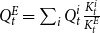 $Q^E_t = \sum _i Q_t^i\frac {K^i_t}{K_t^E}$
, and
 $K^E_t$
the total amount of capital needed by entrepreneurs for their production
 $K^E_t= \sum _i K^i_t$
. Therefore, according to banks, firms with different carbon intensity do not have different probabilities of default. Furthermore, the credit contract will reflect the average level of risk, which will be underestimated for high-carbon-intensive firms (as transition risk is not directly taken into account in this case) and overestimated for low-carbon-intensive firms (who are offered a higher interest rate that covers the transition risk emerging from high-carbon-intensive firms). As capital requirements are a non-linear function of credit risk (
 $PD$
s), then calculating the capital requirements based on the average credit risk will not lead to the same aggregate capital requirements as taking into account firm-specific credit risk.
Bank capital accumulates out of retained earnings from the bank group profits:
 \begin{eqnarray} Bankcap_t = (1-\delta ^{bk})Bankcap_{t-1} +\nu \Pi _t^{bk} \end{eqnarray}
where
 $\delta ^{bk}$
represents the resources used in managing bank capital,
 $\Pi _t^{bk}$
is the overall profit of the banking group which is partially distributed to households as dividends, and
 $\nu$
is the share of retained earning.
The risk weights,
 $rw_t^E$
are computed according to the Basel III IRB approach, as most of the euro area banking system non-financial corporations credit risk is calculated using this approach. According to the Basel III IRB approach, risk weights are defined as follows:
 \begin{align} rw_{t}^{E} & = 12.5 LGD^E \left \{ \Phi \left ( \frac {\Phi ^{-1}(PD_t^E)+(\tau ^{rw^E})^{0.5}\Phi ^{-1}(0.999)}{(1-\tau ^{rw^E})^{0.5} } \right ) - PD_t^E \right \} \end{align}
 \begin{align} \tau ^{rw^E} &= n_1^E \left [ \frac {1-\exp (-n_3^E PD_t^E)}{1-\exp (-n_3^E)}\right ] + n_2^E \left [ 1- \frac {1-\exp (-n_3^E PD^E_t)}{1-\exp (-n_3^E)} \right ] \end{align}
 \begin{align} PD_t^E &= \alpha ^{PD}PD^E_{t-1}+4(1-\alpha ^{PD})F\left (\overline {\omega }_t^E\right ) \end{align}
As aforementioned,
 $PD_t^E$
is the 1-year ahead probability of default of the representative firm, with
 $\alpha ^{PD}$
being the autoregressive coefficient of the PD process and
 $\tau ^{rw^E}$
the asset-value correlation. The parameters
 $n_x,$
with
 $ x=\{1,2,3\}$
are derived from the Basel III regulation for the non-financial corporate sector.
From the maximization problem of the wholesale banks, we obtain the following relation on the interest rate spread between the refinancing rate and the risk-free rate:
 \begin{eqnarray} R_t^{F,E} - R_t = PD^E_{t} LGD^E - \Xi \left (\frac {Bankcap_t}{rw_t^E B_t^{E}} - CR\right ) \left (\frac {Bankcap_t}{rw_t^E B_t^{E}}\right )^2 rw_t^E \end{eqnarray}
We now turn to the second model specification, where banks are required to reflect climate risk in their regulatory constraint. As for the case without climate-prudential policies, the wholesale branch receives deposits from households and chooses the allocation of credit between firms. However, giving credit to firms with different levels of carbon intensity entails different risk weights reflecting individual transition risk. The wholesale branch maximizes the following profit function:
 \begin{align} \max _{\{B_t^{E,i}, D^{H}_t\}} & \sum _i R_t^{F,i} B_t^{E,i} - R_t D^{H}_t - \sum _i PD_t^i LGD^i B_t^{E,i} - \frac {\Xi }{2} \left (\frac {Bankcap_t}{\sum _i rw_t^i B_t^{E,i} } - CR\right )^2 Bankcap_t - \mathbb{T} \end{align}
subject to the following balance sheet identity:
 \begin{eqnarray} \sum _i B_t^{E,i} = D^{H}_t+Bankcap_t \end{eqnarray}
where
 $CR$
is the target capital ratio and
 $rw_t^i$
are the risk weights that apply to each type of firm and are defined following the Basel III IRB approach, similarly to eq. 28–30.
 $\mathbb{T}$
is a sunk cost that banks pay when they have to identify the transition risk of each of their exposures (for example due to the hiring of new experts or the acquisition of data). The probabilities of default of entrepreneurs are different for firms with different degrees of carbon intensity and depend on different idiosyncratic shock thresholds
 $\overline {\omega }_t^i$
. As described in Section 3.2, the threshold value
 $\overline {\omega }^i_t$
depends on the level of carbon emissions, implying a higher probability of default if the firm is more carbon-intensive and, thus, higher credit (transition) risk. As in the case without regulation, bank capital accumulates out of retained earnings from the bank group profits (see eq. 27). Solving the maximization problem, we obtain the following spread between the financing rate for commercial lending branches and the risk-free rate:
 \begin{align} R_t^{F,i}-R_t = PD_t^i LGD^i - \Xi \left (\dfrac {Bankcap_t}{\sum _i rw^i_t B_t^{E,i}} - CR\right ) \left ( \dfrac {Bankcap_t}{\sum _i rw^i_t B_t^{E,i}} \right )^2 rw_t^i \end{align}
where
 $R_t^{F,i}$
is a differentiated financing rate reflecting the specific firms’ transition risk.
3.6.2. The commercial lending branch
As for wholesale branch, we first present the commercial lending branch for the model specification without climate-prudential policies before outlining the changes that are made to the model when we assume that banks have to identify firms on the basis of their carbon intensity. Commercial lending branches issue credit to entrepreneurs without distinguishing between different types of firms. These branches, which obtain funds from the wholesale part of the group, are also in perfect competition and have zero profits in equilibrium. Their profit maximization is given by:
 \begin{eqnarray} \!\!\max _{R_t^E} \!\int _0^{\infty } \frac {\left(1 + R_{t-1}^E\right) B_{t-1}^{E} - \left(1 + R_{t-1}^{F,E}\right)B_{t-1}^{E}}{1+\pi _t} P_t dF\left (\omega _t^E\right ) - \rho \!\!\int _0^{\overline {\omega }_t^E} \!\! (1-\delta )Q_t^EK_{t-1}^E \omega _t^E dF\left (\omega _t^E\right )\,\,\, \end{eqnarray}
where
 $\rho \int _0^{\overline {\omega }_t^E} (1-\delta )Q_t^E K_{t-1}^E \omega _t^E dF\left (\omega _t^E\right )$
are the (real) expected monitoring costs paid by the bank to seize collateral in case of the entrepreneur’s default on its loan commitment. From the zero profit condition, the lending rate applied to the entrepreneur by the commercial lending bank is given by:
 \begin{eqnarray} R^E_{t-1} = R^{F,E}_{t-1} + \frac {1+\pi _t}{B_{t-1}^E P_t}\left [H\left(\overline {\omega }_t^E\right)-G\left(\overline {\omega }_t^E\right)\right ](1-\delta )Q_t^E K_{t-1}^E \end{eqnarray}
As banks do not distinguish between firms, in equilibrium the same financing conditions will be proposed to all types of firms, i.e.,
 $R^{E,i}_t=R^E_t,\ \forall i$
.
We now turn to the model specification with climate-prudential regulation. Without loss of generality, but keeping calculations simpler, each commercial lending branch specializes in giving credit to only one type of firm. As in the case without prudential policies, the commercial lending branches are in perfect competition and have zero profits in equilibrium. They get funds from the wholesale branch and distribute credit to entrepreneurs. Similarly to the model without climate policy, for each type of credit contract, the maximization problem of each commercial lending branch can written as:
 \begin{eqnarray} \!\!\!\!\max _{R_t^{E,i}} \!\int _0^{\infty }\! \frac {\left(1 + R_{t-1}^{E,i}\right) B_{t-1}^{E,i} - \left(1 + R_{t-1}^{F,i}\right)B_{t-1}^{E,i}}{1+\pi _t} P_t dF\left (\omega _t^i\right ) - \rho \!\int _0^{\overline {\omega }_t^i}\!\! (1-\delta )Q_t^i K_{t-1}^i \omega _t^i dF\left (\omega _t^i\right ) \end{eqnarray}
From which we obtain:
 \begin{eqnarray} R^{E,i}_{t-1} = R^{F,i}_{t-1} + \frac {1+\pi _t}{B_{t-1}^{E,i} P_t}\left [H\left(\overline {\omega }_t^i\right)-G\left(\overline {\omega }_t^i\right)\right ](1-\delta )Q_t^i K_{t-1}^i \end{eqnarray}
This implies that in equilibrium different financing conditions will be proposed to each firm type.
4. The Need of Climate-Prudential Policies
Our objective is to use the two models described above to show the need of explicitly incorporating climate risks in the capital framework for banks. To do so, we compare the model setting in which no such policies are implemented with a setting where these policies are enforced, requiring banks to differentiate between firms based on their carbon intensity when calculating capital requirements. It is important to note that this paper does not delve into the specifics of a particular macro- or microprudential policy to achieve this outcome but rather highlights the broader necessity of such policies.
In what follows, we first present the calibration of the models and then we analyze the results obtained when comparing the two model specifications.
4.1. Calibration
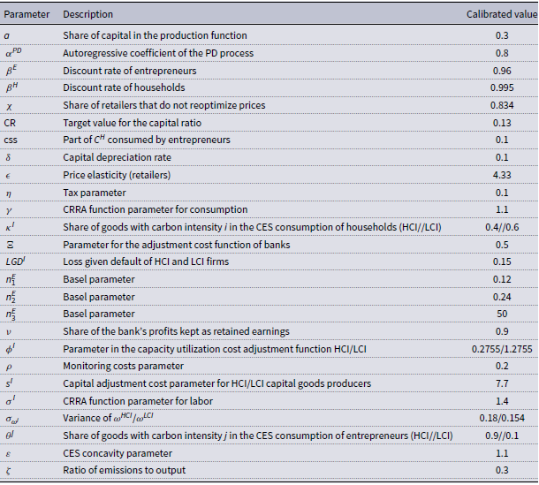
The calibrated values of most parameters are drawn from Darracq-Pariès et al. (Reference Darracq-Pariès, Kok and Rancoita2019) and Darracq-Pariès et al. (Reference Darracq-Pariès, Kok and Rodriguez-Palenzuela2011), as detailed in Appendix B, Table B1. Given that our economy differs slightly from the settings of these papers, some adjustments are introduced. In particular, while the cited works distinguish between firms across different sectors, our framework focuses on firms operating within the same sector but exhibiting different degrees of carbon intensity. To capture this distinction, we calibrate the two types of entrepreneurs differently in terms of their risk profiles (
 $\sigma _{\omega ^i}$
) and the costs of acquiring and adjusting capital for production (
 $\phi ^i$
). We also differentiate between the share of green and more polluting goods in households’ consumption baskets (
 $\kappa ^{LCI}$
and
 $\kappa ^{HCI}$
) and the applicable carbon tax (
 $\eta$
).
Specifically, the parameter
 $\sigma _{\omega ^{i}}$
is calibrated in previous literature (see Darracq-Pariès et al. (Reference Darracq-Pariès, Kok and Rancoita2019)) to match the steady-state probability of default for each entrepreneur type. While there is a growing body of work examining sustainability as a long-term risk factor for corporate viability (Gao et al. (Reference Gao, Li, Wang and Zhong2021), Li et al. (Reference Li, Zhang and Zhao2022), Kanno (Reference Kanno2023)), only Ferriani and Pericoli (Reference Ferriani and Pericoli2024) provide some quantitative evidence on the impact of higher ESG scores on credit risk, which largely corresponds to less carbon-intensive production. Based on this evidence, we adopt the value of
 $\sigma _{\omega ^{LCI}}$
(0.154) from Darracq-Pariès et al. (Reference Darracq-Pariès, Kok and Rancoita2019) and set
 $\sigma _{\omega ^{HCI}}$
to a higher value (0.18) to account for the higher riskiness of HCI entrepreneurs. This calibration ensures that the difference in steady-state default probabilities between HCI and LCI entrepreneurs aligns with the estimates of Ferriani and Pericoli (Reference Ferriani and Pericoli2024), who find that a one-standard-deviation increase in the ESG score is associated with up to a
 $15\%$
reduction in the average probability of default.
Similarly, the adjustment cost parameter for HCI entrepreneurs,
 $\phi ^{HCI}= 0.2755$
, mirrors the value in Darracq-Pariès et al. (Reference Darracq-Pariès, Kok and Rancoita2019), whereas
 $\phi ^{LCI} = 1.2755$
is calibrated to be marginally higher. As discussed in Section 3.2, the higher value for
 $\phi ^{LCI}$
reflects the greater technological and operational constraints faced by cleaner production technologies. The parameter
 $\phi ^i$
does not affect the steady state of the model, since the adjustment cost function equals one in steady state. However,
 $\phi ^i$
influences the sensitivity of the model’s impulse response functions, particularly the lending response, as it impacts the cost of capital and, consequently, firms’ borrowing needs.
Finally, the share of green (polluting) goods in households’ consumption baskets,
 $\kappa ^{LCI}$
(
 $\kappa ^{HCI}$
), is set to 0.6 (0.4) to align with data presented in Figure 1.
In terms of environmental dimension, we use the emission-to-output ratio for the Euro Area,
 $\zeta = 0.3$
, as estimated by Benmir and Roman (Reference Benmir and Roman2020). The tax level,
 $\eta$
, is set to
 $10\%$
such that overall taxes collected on emissions are
 $3\%$
of total production of HCI firms.
Admittedly, the calibration of these key parameters for high- and low-carbon-intensity firms is constrained by the very limited empirical evidence available in the literature. Quantitative studies on this topic remain scarce, and our primary objective is not to provide precise quantitative policy estimates but rather to demonstrate—qualitatively—the necessity of climate-related prudential regulation. To strengthen this point, we conduct extensive robustness checks, reported in Section 5, which show that our main findings are not driven by a specific parametrization. Instead, they hold consistently across a wide and plausible range of parameter values. This provides strong evidence that the core mechanisms identified in the paper are robust and economically relevant.
It is important to stress that the main results of the paper hinge on the non-linearity of the risk-weighted assets formula. In the absence of prudential policies, banks do not distinguish between the two types of firms or their idiosyncratic shocks; instead, they calculate risk weights based on the average firm. By contrast, under climate-prudential policies, risk-weighted assets are computed as a weighted sum of exposures, where risk weights are tailored to the specific carbon intensity of each firm.
4.2. Results
To make the case for introducing climate-prudential policies, we compare the results of the two versions of the model described above—with and without climate-prudential policy intervention.
Figure 2 provides a comparison of steady-state values for various financial variables and for the output of LCI and HCI firms. The bar charts highlight how the introduction of climate-prudential regulation leads to better results for the financial and real sectors. However, there are some caveats to our analysis. First, the model does not have an endogenous level of target capital ratio, and we assume in both cases that this ratio has the same level. In addition, the relative preference of consumers for the two types of products is assumed not to change between the two cases.
Keeping this in mind, we observe that the level of bank capital is higher without climate-prudential policies, as overall there is more risk (lending to the more carbon-intensive firms is higher) implying that banks allocate capital more efficiently when they explicitly consider transition risk. Provisions to cover credit risk losses are about
 $9\%$
lower relative to the case where banks are not submitted to climate-prudential policies as more losses than expected materialize and banks do not correctly internalize the credit risk of their exposures. This result can be explained by the higher steady-state default rates without climate-prudential policies.Footnote
20
When climate-prudential policies apply, the steady-state lending to HCI firms is lower as they are explicitly identified as being riskier, whereas LCI firms receive more credit. This is an important result as it implies that if banks were to fully internalize transition risk, they would have less exposures to HCI firms. Overall credit to the real economy increases when climate-prudential policies are implemented.
Finally, the different allocation of lending between the two institutional settings is also reflected in the output of the two types of firms. The share of productions of HCI firms decreases with respect to the case where no climate-prudential policy is enforced. The opposite is true for LCI firms who benefit from better credit conditions and produce more when climate policy is enforced.
Steady state comparison policy [p] and no-policy [np] case.
Note: The bars represent the ratio (or difference) between the steady-state value from the model where green prudential regulation in enforced with respect to the value from the model where prudential regulation does not take climate transition risk into account.
 $\Delta \%$
is defined as (p-np)/np, pp is defined as (p-np)

We next turn to the analysis of impulse response functions. As outlined in Section 3.2, we model the transition risk shock as a shock to the emission tax, which affects in turn the riskiness of HCI firms,
 $\sigma _{\omega ^{HCI}}$
. This correlation captures additional effects that a sudden increase in the tax rate could have on firms. For the analysis, we calibrate the emission tax shock such that the tax increases by 10%, while the riskiness of entrepreneurs rises by one standard deviation. This calibration allows for a meaningful comparison of our results with those from more conventional macroprudential models.
Figure 3 shows how financial variables respond to an unexpected transition risk shock. We start by looking at the overall dynamics of the model. The shock leads first to an increase in the probability of default of HCI firms. This increase is identical across the policy and no-policy models, as both the initial shocks and all structural parameters are the same in the two scenarios. The higher default risk of these firms increases their financing cost which in turn reduces the amount of credit they can obtain from the bank. When no distinction is made by banks between HCI and LCI firms in terms of transition risk (no policy), lending to LCI firms decreases as well, implying that this type of firms are penalized even if their default risk does not change. The drop in lending can also be explained by the financial constraints that banks have once losses materialize. Indeed, risk-sensitive regulation calls for higher capital requirements when PDs increase, binding the bank to reduce its credit activity. Moreover, provisions considerably increase (up to 10% of their steady-state value) in reaction to the rise in the PD of polluting firms, as more firms default on their credit engagements. When no climate-prudential policy is implemented, the common equity tier 1 ratio (CET1) decreases. This can be explained by the fact that the higher default rate of HCI firms implies not only losses to bank capital but also higher total risk-weighted assets, with risk weights on both high- and low-carbon-intensive firms increasing in the no-policy scenario. Note that the impact on bank capital is limited as banks need to obey capital requirements, but the increase in the PD of polluting firms has a rather persistent impact on risk-weighted assets.
Impulse response functions for the financial sector [lending: in % deviation from the steady state; all other variables: pp difference from the steady state].
Note: The figure presents the IRFs of financial variables to a transition risk shock implying 10% higher emission taxes and 1 standard deviation shock to
 $\sigma _{\omega ^{HCI}}$
, the riskiness of HCI firms.

When comparing the two models—with and without climate-prudential policies—we can see that the introduction of climate-prudential policies weakens the negative effect of the transition shock.Footnote 21 In response to an increase in the riskiness of the more polluting firms, banks deleverage more with respect to this type of firms when the policy is implemented. This clearly shows that regulation increases the sensitivity of banks to transition risk. At the same time, lending to LCI firms is rather stable with respect to its steady-state value when climate-prudential policies are implemented. The penalty seen before for this type of firm is thus alleviated with climate-prudential policies in place. Notice that when banks are not obliged to distinguish between HCI and LCI firms, the lending rate is the same for both of them. With policy intervention, LCI firms obtain more favorable financing conditions than HCI firms for which the increase in the lending rate is more important than in the model without climate-prudential policies. Enforcing climate-related prudential policies leads thus to more equitable financing conditions, riskier firms having to pay higher interest rates on their credit. Total lending decreases less under the policy case (mainly driven by credit to more polluting companies). The difference is of approximately 15 basis points at its maximum, implying less consequences on the real economy when climate-prudential policy is in place. Furthermore, in the case where these type of policies are enforced, we assume that regulation is relaxed with respect to polluting firms if a transition shock would materialize. This translates into a release of capital requirements allowing banks to diverge from the steady state ratio with lower bank capital for several periods. At the same time, risk-weighted assets decrease for the first period as lending to HCI firms decreases, to increase immediately afterwards when the decrease in lending is more than compensated by the increase in the risk weights applied to polluting firms. In the simulations, it is assumed that the relaxation of prudential policies is in magnitude of about 30 bps (which is close but below the release of other capital requirements in previous crises). Due to the relaxation of the capital requirements, in the policy case the CET1 ratio slightly increases in the beginning of the simulation period, to decrease immediately afterwards. Overall, implementing climate-prudential policies to account for transition risk seems beneficial for the financial system as banks better internalize the actual credit risk of their exposures. Different values of the capital requirements release would lead to similar results. However, in this simulation we do not provide a precise estimate of the size of the excess in credit risk generated by transition risk. As mentioned earlier, the model is calibrated with values already used in the literature but due to lack of data we cannot estimate the distribution of transition risk shocks. In the current example, we assume that the size of the transition risk shock is of half the standard deviation of the calibrated riskiness of firms in Darracq-Pariès et al. (Reference Darracq-Pariès, Kok and Rancoita2019). This reflects the idea that transition risk is currently a less relevant source of credit risk, but at the same time it allows us to work with realistic magnitudes despite the lack of data for the calibration.
Figure 4 shows the response of the real economy for the above mentioned exercise.Footnote 22 As expected, the increase in transition risk of HCI borrowers translates in lower total output and investment, reflecting the deleveraging of banks and the higher cost of credit in both sectors. In the case where climate-prudential policies are implemented, the impact on the real economy is better contained, as investment decreases less. The decline in output is mainly driven by the investment level, as consumption of both low- and high-carbon-intensive goods tends to support output (recall that it is assumed here that consumers do not change their preferences). Looking at the production breakdown, it is relevant to notice that the output of polluting firms decreases a lot more when climate-prudential policy is implemented, whereas the production of less polluting goods is only slightly impacted. However, without policies in place the production in both sectors would considerably diminish, as banks would deleverage in a similar way on all exposures. Finally, as inflation and output diminish in the economy, the monetary authority reduces its interest rate, but the impact is less pronounced when explicit transition risk policies are implemented.
Impulse response functions for the real sector [% deviation from the steady state, CPI and risk-free rate in pp. difference from the steady state].
Note: The figure presents the IRFs of real economic variables to a transition risk shock implying 10% higher emission taxes and 1 standard deviation shock to
 $\sigma _{\omega ^{HCI}}$
, the riskiness of HCI firms.

In order to highlight the stabilization trade-offs and show more general results, we compare the efficiency policy frontiers implied by the models with and without climate-prudential policies. The efficiency policy frontier (EPF) portrays the surface where it is not possible to attain lower variance in one objective variable without increasing the one of the others. In the case under consideration, the efficiency policy frontiers reflect the three target variables of the monetary and macroprudential policy authorities: inflation, output gap, and credit volatilities. The efficiency policy frontiers abstracts from the specific loss function and the strategic interaction between the monetary and macroprudential authorities, and the ‘best’ allocation is given by the intersection with the efficiency policy frontiers and the authorities loss function/s. We conducted two simulations assuming either that climate-prudential policies are implemented or that they are not. In each case, we optimized the monetary policy rule in terms of the coefficient of the inflation gap and of the output gap. The model does not specify any particular rule for the climate-prudential policies, but we assume either that they are not implemented at all or that they allow a perfect identification of transition risk. In all cases, we activate the transition shocks. The resulting standard deviations for inflation, output gap, and credit for each coefficient combination are illustrated in Figure 5. Depending on the assumptions about the loss function/s of the monetary authority and the activation of climate-prudential policies, we can select a different point on each efficiency policy frontier to be the best.
Efficiency frontier between output-lending policy outcomes (left) and inflation-output outcomes (right).
Note: The chart represents the efficiency policy frontier for given shocks to borrower riskiness. The efficiency frontier portrays, for all sets of policymaker’s preferences, the lending, output and inflation volatilities implied by the corresponding optimized rules.

In Figure 5, we can observe that the activation of climate-prudential policies leads overall to lower output, inflation, and lending volatility in equilibrium for any optimal monetary policy rule. We can derive some relevant policy conclusions from Figure 5 even without being specific about the loss functions of the policy authorities or about the strategic interactions among the authorities. Introducing climate-prudential policies Pareto dominates the institutional configuration without them and this induces an inward shift in the efficiency frontier. Relevantly, this also enables monetary policy to achieve a superior performance in terms of macroeconomic stabilization.
5. Robustness
As a first robustness check, we set all parameters that differ across the two types of firms in the baseline calibration to the same values. The purpose of this exercise is to demonstrate that our main results are not driven by specific calibration choices regarding the heterogeneity between HCI and LCI firms, but rather by the structural features of the two models we compare. In Appendix D.1, Figures D1 and D2, we illustrate the key impulse responses to a shock in the riskiness of HCI firms under this assumption, namely that all key parameters distinguishing the two types of firms (
 $\sigma _{\omega ^{i}}$
,
 $\phi ^{i}$
, and
 $\kappa ^{i}$
) are set equal. The resulting impulse responses are very similar to those reported in the main results, although the magnitude of the wedge between them changes. This confirms that our qualitative findings do not hinge on the particular calibration of firm heterogeneity.
The second robustness analysis focuses on the parameter
 $\sigma _{\omega ^i}$
. More sustainable production technologies with low carbon intensity are expected to increase the viability of firms. This is supported by recent studies providing preliminary empirical evidence that firms with better ESG scores exhibit lower credit risk (Ferriani and Pericoli (Reference Ferriani and Pericoli2024)). In our model, the parameter
 $\sigma _{\omega ^{i}}$
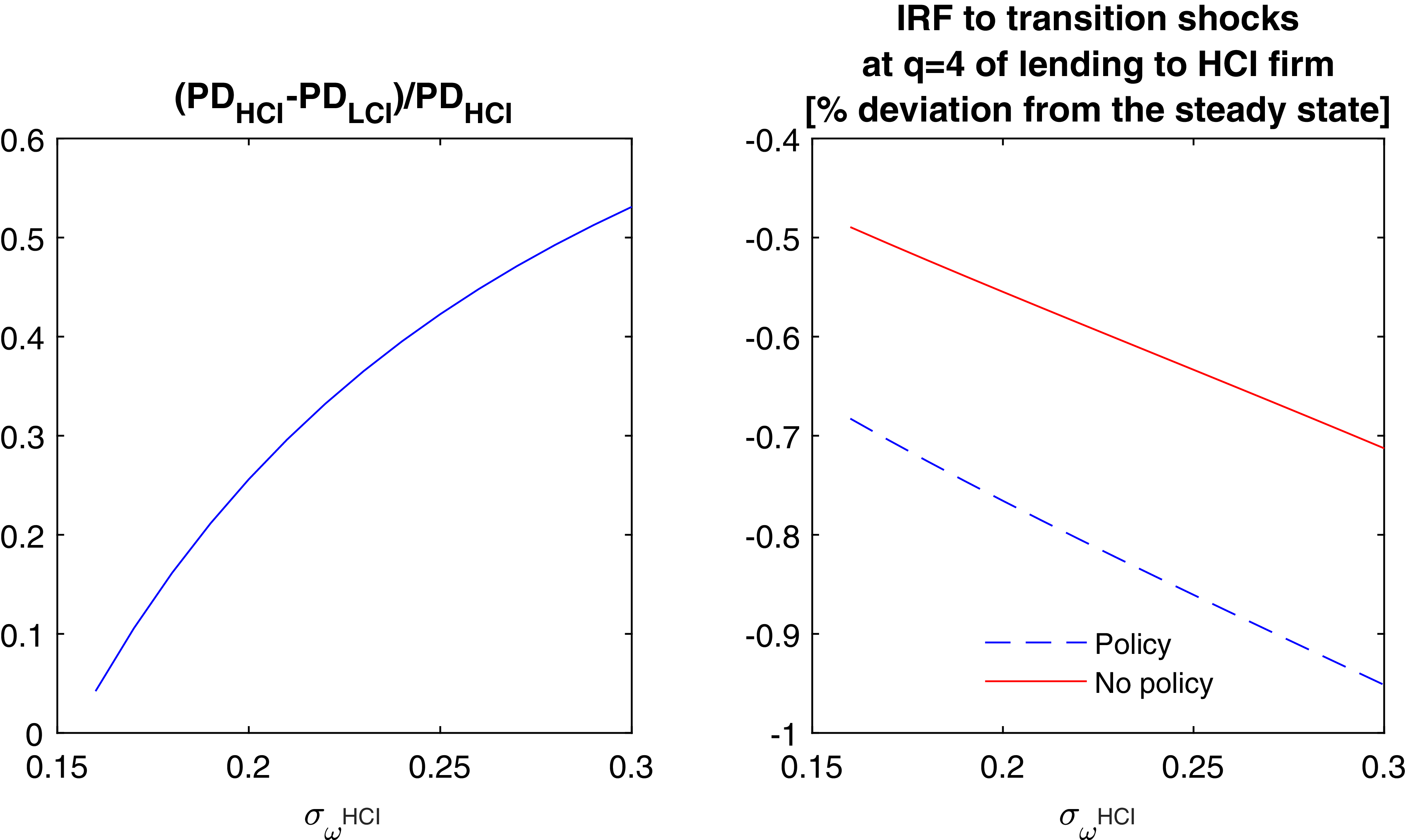
plays a key role in determining the probability of default of different types of entrepreneurs in equilibrium. As a robustness analysis, we first illustrate how variations in
 $\sigma _{\omega ^{HCI}}$
affect the steady-state difference in default probabilities between HCI and LCI firms, while keeping
 $\sigma _{\omega ^{LCI}}$
fixed at
 $0.15$
(following the literature). Figure D3 (left panel) in Appendix D.2 shows the percentage difference in PDs at steady state as
 $\sigma _{\omega ^{HCI}}$
ranges from
 $0.15$
(equal to
 $\sigma _{\omega ^{LCI}}$
) up to
 $0.3$
. Setting
 $\sigma _{\omega ^{HCI}}$
at
 $0.3$
would imply that LCI firms’ steady-state PD is
 $50\%$
lower than that of HCI firms, well above the
 $15\%$
long-term difference suggested by Ferriani and Pericoli (Reference Ferriani and Pericoli2024). For the main calibration, we therefore set
 $\sigma _{\omega ^{HCI}}=0.18$
, while the upper bound of our robustness checks more than doubles this value.
The right panel of Figure D3 presents the quarter 4 impulse responses of lending to HCI firms following a climate transition shock. This variable is directly affected by the calibration of
 $\sigma _{\omega ^{HCI}}$
and, in turn, drives most of the other IRFs in the model. The quarter shown corresponds to the period in which the difference between the policy and no-policy cases is largest. The impulse responses are displayed over the same range as in the left panel, i.e.,
 $\sigma _{\omega ^{HCI}} \in [0.15, 0.3]$
. The figure shows that, while the parameter value affects the overall level of the elasticity, the gap between the policy and no-policy models increases only slightly for very high values of
 $\sigma _{\omega ^{HCI}}$
, and this increase is monotonic. This indicates that our qualitative results are robust and hold across a broad and plausible range of
 $\sigma _{\omega ^{HCI}}$
values.
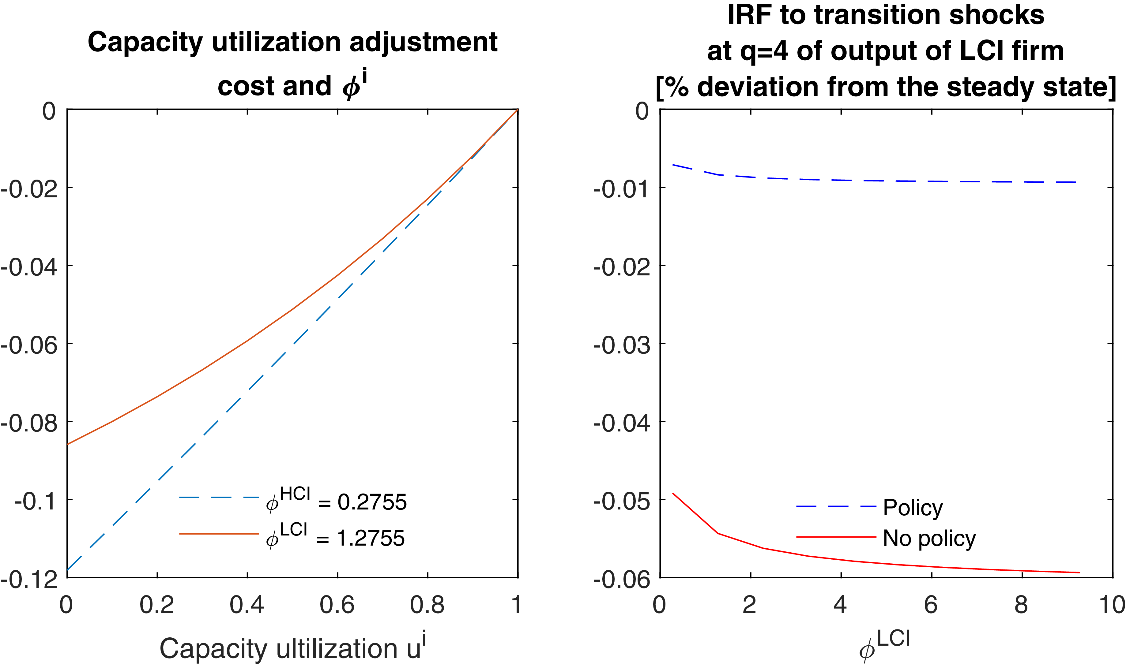
Our third robustness check concerns the adjustment cost parameter
 $\phi ^{i}$
. In Appendix D.3, we illustrate how the adjustment cost function depends on the parameter
 $\phi ^i$
. While the value of
 $\phi ^{HCI}$
is anchored to calibrated values in the literature, we set
 $\phi ^{LCI}$
at a higher value. In Figure D4 (left), we illustrate how the adjustment cost function varies with the parameter
 $\phi ^i$
. As shown, at high levels of capacity utilization (i.e., near the steady state), the differences in adjustment costs generated by
 $\phi ^i$
are negligible. Given that transition risk is not expected to cause large disruptions—consistent with the economic reasoning discussed in the main text and the calibration of
 $\sigma _{\omega }^{HCI}$
—we expect that variations in this parameter will not significantly affect the simulations presented in this paper.
We also report in Appendix D.3 the sensitivity of output impulse responses (which is the variable most directly affected by the parameter) to variations in
 $\phi ^{LCI}$
for both the policy and no-policy models. Overall, both the level and the gap between the two IRFs change only marginally and monotonically, even for large variations in
 $\phi ^{LCI}$
. This suggests that the choice of this parameter is largely neutral for the overall outcomes of the model.
Finally, the calibration of
 $\kappa ^i$
in the CES preference function affects the relative demand elasticities of HCI and LCI goods, and consequently the results. This parameter is calibrated to match aggregate figures on overall lending to both types of sectors, which serve as a proxy for aggregate production. The model is a simplified representation of reality, and in practice, there is a continuum of carbon intensities for the same product, making a precise calibration challenging. We therefore provide robustness tests for this parameter in Appendix D.4. Indeed, Figure D5 (left and right panels) shows the impulse responses at the peak quarter (q= 4) of output for LCI and HCI firms across all plausible values of
 $\kappa ^{LCI}$
, for both the policy and no-policy models.Footnote
23
The results vary monotonically with
 $\kappa ^{LCI}$
, indicating that the conclusions regarding the Pareto improvement due to the introduction of prudential policies hold across all reasonable parameterizations.
6. Conclusion
In this paper, we underline the need of implementing climate-prudential policies to address transition risk in the banking sector. Unlike most previous literature, our conclusions focus exclusively on prudential and financial stability considerations, rather than on climate change mitigation objectives set by authorities. Using a DSGE model with heterogeneous firms and financial frictions, our analysis reveals that without climate-prudential policies, banks fail to adequately cover credit risk associated with transition risks, leading to more severe macroeconomic output decline when risk materialize. Indeed, when transition risks are not accounted for, banks disproportionately allocate resources to high-carbon-intensive firms, underestimating their credit risks. This mispricing not only undermines financial stability but also hinders efficient capital allocation. Conversely, the introduction of climate-prudential policies—such as differentiated capital requirements or enhanced transparency measures—encourages banks to internalize transition risks. Such measures result in improved credit risk assessments, reduced exposure to high-risk firms, and more stable financial and economic outcomes. Introducing climate-prudential measures proves to be Pareto superior, reducing credit volatility and enhancing macroeconomic stabilization.
Our work contributes significantly to the current policy debate, providing a clear argument for the adoption of climate-prudential policies to secure future financial stability. By identifying areas for improvement in current banking practices regarding transition risk, we offer valuable insights for policymakers aiming to strengthen financial systems against climate-related disruptions. While our analysis offers valuable insights, it is not without limitations. Specifically, we abstract from the design of particular policy measures aimed at addressing transition risk, instead assuming that the implemented policy results in the full internalization of transition risk by banks. As such, future research could extend this framework by incorporating specific policies and assessing their effectiveness. Additionally, future studies could broaden the scope to include physical risks alongside transition risks, thereby providing a more comprehensive understanding of the overall effectiveness of climate-prudential policies. Furthermore, it could be beneficial to explore the integration of climate-prudential policies with other regulatory frameworks, such as monetary and fiscal policies, to assess their combined effect on overall economic stability. Investigating the role of technological innovation and green finance in mitigating transition risks could also yield valuable insights for the discussion on how to design climate-prudential policies.
Acknowledgements
We would like to thank the two anonymous referees for comments that greatly improved the paper, as well as the editors of the journal. We express our gratitude to the participants of the Directorate General-Macroprudential Policy and Financial Stability Seminar Series for their insightful comments and suggestions. We also thank attendees of the National Bank of Romania internal seminar, the BETA Cournot seminar, the JIR Annual Conference, and the INFER Workshop on Global Changes, International Trade, and Health in Bordeaux, France, for their valuable feedback. The views presented in this paper are solely those of the authors and do not necessarily reflect the opinions of the European Central Bank. Any remaining errors are ours.
Competing interests
The authors declare none.
Appendix A. Model calculations
A.1. Households FOCs
The Lagrangian of the households writes:
 \begin{align} \mathcal{L}_t^H &= \mathbb{E}_{t}\Bigg \{ \sum _{t=0}^{\infty } \beta ^{H^t} \Bigg [ \Bigg (\frac {C_t^{H^{1-\gamma }}}{1-\gamma } - \sum _i \overline {L^i}\frac {L_t^{i^{1+\sigma ^i}}}{1+\sigma ^i}\Bigg ) \Bigg .\Bigg . \nonumber \\ &\quad\Bigg .\Bigg . - \lambda _t^{H,BC}\Bigg ( \sum _i P_t^i C_t^{H,i}+ P_t D_t^H -P_t \frac {1+R_{t-1}}{1+\pi _t}D_{t-1}^H - \sum _i w_t^i L_t^i - \Pi _t^H - G_t \Bigg )\Bigg ] \Bigg \} \end{align}
with:
 \begin{eqnarray} C_t^H &=& \left [ \sum _i \epsilon _t^{c,i}\kappa ^{i^{\frac {1}{\varepsilon }}} C_t^{{H,i}^{\frac {\varepsilon -1}{\varepsilon }}} \right ]^{\frac {\varepsilon }{\varepsilon -1}} \end{eqnarray}
where
 $i=\{HCI,LCI\}$
. The maximization problem implies the following FOCs:
 \begin{align} C_t^{H,i} &\,:\, \epsilon _t^{c,i}\kappa ^{i^{\frac {1}{\varepsilon }}} C_t^{{H}^{\frac {1}{\varepsilon }-\gamma }} C_t^{{H,i}^{-\frac {1}{\varepsilon }}} - \lambda _t^{H,BC}P_t^i = 0 \end{align}
 \begin{align} D_t^H &\,:\, P_t\lambda _t^{H,BC} - \beta ^H \mathbb{E}_{t}\left ( \lambda _{t+1}^{H,BC} P_{t+1}\frac {1+R_t}{1+\pi _{t+1}}\right ) = 0 \end{align}
 \begin{align} L_t^i &\,:\, -\overline {L^i} L_t^{i^{\sigma ^i}} + \lambda _t^{H,BC}w_t^i = 0 \end{align}
 \begin{align} \lambda _t^{H,BC} &\,:\, \sum _i P_t^i C_t^{H,i} +P_t D_t^H -P_t \frac {1+R_{t-1}}{1+\pi _t}D_{t-1}^H - \sum _i w_t^i L_t^i - \Pi _t^H - G_t = 0 \end{align}
At the steady state, the FOCs imply the following:
 \begin{align} C^{H,i} &\,:\, \kappa ^{i^{\frac {1}{\varepsilon }}} C^{{H}^{\frac {1}{\varepsilon }-\gamma }} C^{{H,i}^{-\frac {1}{\varepsilon }}} - \lambda ^{H,BC}P^i = 0 \end{align}
 \begin{align} D^H &\,:\, 1 - \beta ^H (1+R) = 0 \end{align}
 \begin{align} L^i &\,:\, - \overline {L^i} L^{i^{\sigma ^i}} + \lambda ^{H,BC}w^i = 0 \end{align}
 \begin{align} \lambda ^{H,BC} &\,:\, \sum _i P^i C^{H,i} - P\ R\ D^H - \sum _i w^i L^i - \Pi ^H - G = 0 \end{align}
From eq. A7, we obtain the following condition for each pair of goods:
 \begin{eqnarray} \frac {C^{H,i}}{C^{H,j}} &=& \frac {\kappa ^i}{\kappa ^j}\left ( \frac {P^j}{P^i} \right )^{\varepsilon } \end{eqnarray}
A.2. Entrepreneur FOCs
The Lagrangian of each type of entrepreneur
 $i=\{HCI,LCI\}$
writes:
 \begin{eqnarray} \mathcal{L}_t^{E,i} &=& \mathbb{E}_{t}\Bigg \{ \sum _{t=0}^{\infty } \beta ^{E^t} \Bigg \{ \frac {C_t^{{E,i}^{1-\gamma }} }{1-\gamma } - \lambda _t^{E,i,BC}\Bigg [ \sum _j P_t^j C_t^{E,i,j} \Bigg .\Bigg .\Bigg .\nonumber \\ &&\Bigg .\Bigg .\Bigg . + Q_t^i\left (K_t^i - (1-\delta )K_{t-1}^i \right ) + w_t^i L_t^i + \Phi _i(u_t^i)K_{t-1}^i + H(\overline {\omega }_t^i)(1-\delta )Q_t^i K_{t-1}^i \Bigg .\Bigg .\Bigg . \nonumber \\ && \Bigg .\Bigg .\Bigg . +\eta ^i\zeta \epsilon _t^i \left (u_t^i K_{t-1}^i\right )^a \left (L_t^i\right )^{1-a} - \mu _t^i P_t^i \epsilon _t^i \left (u_t^i K_{t-1}^i\right )^a \left (L_t^i\right )^{1-a} - P_t B_t^{E,i}\Bigg ]\Bigg .\nonumber \\ &&\Bigg .-\lambda _t^{E,i,PC}\Bigg [ \frac {1+R_{t-1}^{F,i}}{1+\pi _t}P_t B_{t-1}^{E,i} - (1-\delta )Q_t^i K_{t-1}^i G(\overline {\omega }_t^i)\Bigg ]\Bigg \}\Bigg \} \end{eqnarray}
with:
 \begin{eqnarray} C_t^{E,i} &=& \left [ \sum _j \theta ^{j^{\frac {1}{\varepsilon }}} C_t^{{E,i,j}^{\frac {\varepsilon -1}{\varepsilon }}} \right ]^{\frac {\varepsilon }{\varepsilon -1}} \end{eqnarray}
and where:
 \begin{align} H(\overline {\omega }_t^i) &= \mathcal{N_{CDF}}\left ( \frac {log(\overline {\omega }_t^i)-0.5 \sigma _{\omega ^i}^2}{\sigma _{\omega ^i}} \right ) + \overline {\omega }_t^i \left (1-\mathcal{N_{CDF}}\left ( \frac {log(\overline {\omega }_t^i)+0.5 \sigma _{\omega ^i}^2}{\sigma _{\omega ^i}} \right ) \right ) \end{align}
 \begin{align} G(\overline {\omega }_t^i) &= (1-\rho )\mathcal{N_{CDF}}\left ( \frac {log(\overline {\omega }_t^i)-0.5 \sigma _{\omega ^i}^2}{\sigma _{\omega ^i}} \right ) + \overline {\omega }_t^i \left (1-\mathcal{N_{CDF}}\left ( \frac {log(\overline {\omega }_t^i)+0.5 \sigma _{\omega ^i}^2}{\sigma _{\omega ^i}} \right ) \right ) \end{align}
The maximization problem implies the following FOCs:
 \begin{align} C_t^{E,i,j} &\,:\, \theta ^{j^{\frac {1}{\varepsilon }}} C_t^{{E,i}^{\frac {1}{\varepsilon }-\gamma }} C_t^{{E,i,j}^{-\frac {1}{\varepsilon }}} - \lambda _t^{E,i,BC}P_t^j = 0 \end{align}
 \begin{align} L_t^i &\,:\, w_t^i +\eta ^i\zeta \epsilon _t^i \left (u_t^i K_{t-1}^i\right )^a (1-a) \left (L_t^i\right )^{(1-a)-1} \nonumber \\ &\quad - \mu _t^i P_t^i\epsilon _t^i \left (u_t^i K_{t-1}^i\right )^a (1-a)\left (L_t^i\right )^{-a} = 0 \end{align}
 \begin{align} K_t^i &\,:\, - \lambda _t^{E,i,BC}Q_t^i - \beta ^E \mathbb{E}_{t} \bigg [\lambda _{t+1}^{E,i,BC}\Big [-Q_{t+1}^i (1-\delta ) + \Phi _B(u_{t+1}^i) \Bigg .\Bigg . \nonumber \\ &\quad\Bigg .\Bigg . + H(\overline {\omega }_{t+1}^i)(1-\delta )Q_{t+1}^i + \eta ^i\zeta \epsilon _{t+1}^i \left (u_{t+1}^i \right )^a \left (L_{t+1}^i\right )^{1-a} a \left (K_t^i\right )^{a-1} \Bigg .\Bigg . \nonumber \\ &\quad\Bigg .\Bigg . - \mu _{t+1}^i P_{t+1}^i \epsilon _{t+1}^i \left (u_{t+1}^i \right )^a \left (L_{t+1}^i\right )^{1-a}a \left (K_t^i\right )^{a-1} \Big ]\bigg ] \nonumber \\[5pt] &\quad - \beta ^E \mathbb{E}_{t} \Big [-\lambda _{t+1}^{E,i,PC}(1-\delta )Q_{t+1}^i G(\overline {\omega }_{t+1}^i) \Big ]=0 \\\nonumber \end{align}
 \begin{align} u_t^i &\,:\, \Phi _i'(u_t^i)K_{t-1}^i + \eta ^i\zeta \epsilon _t^i \left (K_{t-1}^i\right )^a \left (L_t^i\right )^{1-a} a \left (u_t^i \right )^{a-1} \nonumber \\[8pt] &\quad - \mu _t^i P_t^i \epsilon _t^i \left (K_{t-1}^i\right )^a \left (L_t^i\right )^{1-a}a\left (u_t^i\right )^{a-1} = 0 \\\nonumber \end{align}
 \begin{align} B_t^{E,i} &\,:\, P_t \lambda _t^{E,i,BC} - \beta ^E \mathbb{E}_{t}\left (\lambda _{t+1}^{E,i,PC}\frac {1+R_t^{F,i}}{1+\pi _{t+1}}P_{t+1}\right ) = 0 \end{align}
 \begin{align} \overline {\omega }_t^i&\,:\, - \lambda _t^{E,i,BC} H'(\overline {\omega }_t^i) + \lambda _t^{E,i,PC} G'(\overline {\omega }_t^i) = 0 \\\nonumber \end{align}
 \begin{align} \lambda _t^{E,i,BC} &\,:\, \sum _j P_t^j C_t^{E,i,j} + Q_t^i\left ( K_t^i -(1-\delta )K_{t-1}^i\right ) \nonumber \\[3pt] &\quad + w_t^i L_t^i + \Phi _i(u_t^i)K_{t-1}^i + H(\overline {\omega }_t^i)(1-\delta )Q_t^i K_{t-1}^i \nonumber \\[5pt] &\quad + \eta ^i\zeta \epsilon _t^i \left (u_t^i K_{t-1}^i\right )^a \left (L_t^i\right )^{1-a} - \mu _t^i P_t^i \epsilon _t^i \left (u_t^i K_{t-1}^i\right )^a \left (L_t^i\right )^{1-a} \\[-8pt]\nonumber \end{align}
 \begin{align}&\quad - P_t B_t^{E,i} = 0 \\[-3pt]\nonumber \end{align}
 \begin{align} \lambda _t^{E,i,PC} &\,:\, \frac {1+R_{t-1}^{F,i}}{1+\pi _t}P_t B_{t-1}^{E,i} - (1-\delta )Q_t^i K_{t-1}^i G(\overline {\omega }_t^i) = 0 \end{align}
At the steady state, the FOCs can be rewritten as:
 \begin{align} C^{E,i,j} &\,:\, \theta ^{j ^{\frac {1}{\varepsilon }}} C^{{E,i}^{\frac {1}{\varepsilon }-\gamma }} C^{{E,i,j}^{-\frac {1}{\varepsilon }}} - \lambda ^{E,i,BC}P^j = 0 \end{align}
 \begin{align} L^i &\,:\, w^i L^i + (1-a) \left ( \eta ^i\zeta Z^i - \mu ^i P^i Z^i \right ) = 0 \end{align}
 \begin{align} K^i &\,:\, - \lambda ^{E,i,BC}Q^i K^i - \beta ^E \bigg [\lambda ^{E,i,BC}\Big [- (1-\delta ) Q^i K^i + \Phi _i(u^i) K^i \Bigg .\Bigg . \nonumber \\[5pt] &\quad\Bigg .\Bigg . + H(\overline {\omega }^i)(1-\delta )Q^i K^i + a \left ( \eta ^i\zeta Z^i - \mu ^i P^i Z^i \right ) \Big ]\bigg ] \nonumber \\[5pt]&\quad - \beta ^E \Big [-\lambda ^{E,i,PC}(1-\delta )Q^i K^i G(\overline {\omega }^i) \Big ]=0 \\[-6pt]\nonumber\end{align}
 \begin{align} u^i &\,:\, \Phi _i'(u^i)u^i K^i + a \left ( \eta ^i\zeta Z^i - \mu ^i P^i Z^i \right ) = 0 \\[-6pt]\nonumber\end{align}
 \begin{align} B^{E,i} &\,:\, \lambda ^{E,i,BC} - \beta ^E \lambda ^{E,i,PC}\left (1+R^{F,i}\right ) = 0 \\[-6pt]\nonumber\end{align}
 \begin{align} \overline {\omega }^i&\,:\, - \lambda ^{E,i,BC} H'(\overline {\omega }^i) + \lambda ^{E,i,PC} G'(\overline {\omega }^i) = 0 \\[-6pt]\nonumber\end{align}
 \begin{align} \lambda ^{E,i,BC} &\,:\, \sum _j P^j C^{E,i,j} + \delta Q^i K^i+ w^i L^i + \Phi _i(u^i)K^i \nonumber \\ &\quad + H(\overline {\omega }^i)(1-\delta )Q^i K^i + \left ( \eta ^i\zeta Z^i - \mu ^i P^i Z^i \right ) - P\ B^{E,i} = 0 \\[-6pt]\nonumber\end{align}
 \begin{align} \lambda ^{E,i,PC} &\,:\, \left (1+R^{F,i}\right ) P B^{E,i} - (1-\delta )Q^i K^i G(\overline {\omega }^i) = 0 \end{align}
From eq. A25, we obtain for any couple of products
 $k,j$
:
 \begin{eqnarray} \frac {C^{E,i,k}}{C^{E,i,j}} &=& \frac {\theta ^k}{\theta ^j}\left ( \frac {P^j}{P^k} \right )^{\varepsilon } \end{eqnarray}
From eqs. A26 and A28 and using the fact that
 $u^i = 1 \Rightarrow \Phi _i'(u^i) = r^{i,SS}$
at the steady state, we obtain:
 \begin{eqnarray} \frac {u^i K^i}{L^i} = \frac {a w^{i}}{(1-a) r^{i,SS}} \end{eqnarray}
which together with the the zero profit condition in eq. 12, implies:
 \begin{align} \mu ^iP^i - T(e_t^i) &= \frac {w^{i^{1-a}}r^{{i,SS}^{a}}}{a^{a} (1-a)^{1-a}} \end{align}
 \begin{align} \Leftrightarrow w^i &= \left ( (\mu ^i P^i-T(e_t^i))r^{{i,SS}^{-a}}a^{a} (1-a)^{1-a} \right )^{1/(1-a)} \end{align}
From eqs. A29 and A30, we obtain:
 \begin{eqnarray} \frac {G'(\overline {\omega }^i)}{ H'(\overline {\omega }^i) } &=& \beta ^E\left (1+R^{F,i}\right ) \end{eqnarray}
In addition using the fact that
 $\Phi _i(u^i) = 0$
at the steady state, we can rewrite eq. A27 as:
 \begin{eqnarray} &&Q ^i K^i [\beta ^E(1-\delta )-1] + \beta ^E(1-\delta ) Q^i K^i \left (\frac {\lambda ^{E,i,PC}}{\lambda ^{E,i,BC}}G(\overline {\omega }^i) - H(\overline {\omega }^i\right ) \nonumber \\ &&\quad -\beta ^E a \left ( \eta ^i\zeta Z^i - \mu ^i P^i Z^i \right ) = 0 \end{eqnarray}
Using the fact that
 $Q^i=1$
and
 $\frac {\lambda ^{E,i,PC}}{\lambda ^{E,i,BC}}=\frac {H'(\overline {\omega }^i)}{G'(\overline {\omega }^i)}$
and that the marginal return to capital from the production,
 $r^{i,SS}$
is
 $(\mu ^i P^i - \eta ^i\zeta ) a K^{i^{a-1}} L^{i^{(1-a)}} = (\mu ^i P^i - \eta ^i\zeta ) aZ^i/K^i$
. We then obtain:
 \begin{align} &[\beta ^E(1-\delta )-1] + \beta ^E(1-\delta ) \left [\frac {H'(\overline {\omega }^i)}{G'(\overline {\omega }^i)}G(\overline {\omega }^i) - H(\overline {\omega }^i)\right ] + \beta ^E r^{i,SS} = 0 \end{align}
 \begin{align} & \Leftrightarrow r^{i,ss} = \frac {1}{\beta ^E} - (1-\delta )-(1-\delta ) \left [\frac {H'(\overline {\omega }^i)}{G'(\overline {\omega }^i)}G(\overline {\omega }^i) - H(\overline {\omega }^i)\right ] \end{align}
A.3. Capital goods producers FOCs
Substituting the law of motion of capital:
 \begin{eqnarray} \max _{\{I_t^i\}} \mathbb{E}_{t}\left \{\sum _{t=0}^{\infty } \beta ^t \Bigg [ Q_t^i \left [ (1-\delta )K_{t-1}^i + \left [1-S\left (\frac {I_t^i}{I_{t-1}^i}\right )\right ]I_t^i - (1-\delta )K_{t-1}^i\right ] - I_t^i \Bigg ] \right \}. \end{eqnarray}
FOC:
 \begin{eqnarray} I_t^i &\,:\, Q_t^i\left [1-S\left (\frac {I_t^i }{I_{t-1}^i}\right ) \right ] - Q_t^i\frac {I_t^i }{I_{t-1}^i} S'\left (\frac {I_t^i }{I_{t-1}^i}\right ) + \beta \mathbb{E}_{t}\left [ Q_{t+1}^i\left (\frac {I_{t+1}^i}{I_t^i}\right )^2 S'\left (\frac {I_{t+1}^i}{I_t^i}\right ) \right ] = 1 \end{eqnarray}
At the steady state, the investment is given by:
 \begin{eqnarray} I^i = \delta K^i \end{eqnarray}
Furthermore, given that
 $S(1) = 0$
and
 $S'(1) = 0$
, from eq. A42, we obtain the price of capital at steady state:
 \begin{eqnarray} Q^i = 1 \end{eqnarray}
A.4. Retailers FOCs
The maximization of the retailers,
 $i=\{HCI,LCI\}$
writes:
 \begin{eqnarray} \max _{\{\tilde {P}_t^i(j)\}} \sum _{k=0}^{\infty } \chi ^k \mathbb{E}_t \left [\lambda ^{r,i}_{t+k}\left [\tilde {P}_t^i(j)- \mu _{t+1}^i P_{t+k}^i \right ]\left ( \frac {\tilde {P}_t^i(j)}{P_{t+k}^i}\right )^{-\epsilon }Y_{t+k}^i\right ] \end{eqnarray}
Proof for the recursive form:
The derivative with respect to
 $\tilde {P}_t^i(j)$
is equal to:
 \begin{align} \tilde {P}_t^i(j) &\,:\, \sum _{k=0}^{\infty } \chi ^k \mathbb{E}_{t} \Bigg \{ \lambda ^{r,i}_{t+k}\left [\left ( \frac {\tilde {P}_t^i(j)}{P_{t+k}^i}\right )^{-\epsilon }Y_{t+k}^i -\epsilon \left (\tilde {P}_t^i(j)- \mu _{t+k}^i P_{t+k}^i \right )\frac {(\tilde {P}_t^i(j))^{-\epsilon -1}}{(P_{t+k}^i)^{-\epsilon }}Y_{t+k}^i \right ] \Bigg \} = 0\quad \end{align}
Equivalently:
 \begin{align} \sum _{k=0}^{\infty } \chi ^k \mathbb{E}_{t}\left \{\lambda ^{r,i}_{t+k}\left [\left ( \frac {\tilde {P}_t^i(j)}{P_{t+k}^i}\right )^{-\epsilon }Y_{t+k}^i - \epsilon \left (\frac {\tilde {P}_t^i(j)}{P_{t+k}^i}\right )^{-\epsilon }Y_{t+k}^i + \epsilon \mu _{t+k}^i \left (\frac {\tilde {P}_t^i(j)}{P_{t+k}^i}\right )^{-\epsilon -1}Z_{t+k}^i \right ] \right \} = 0 \end{align}
Or:
 \begin{eqnarray} \sum _{k=0}^{\infty } \chi ^k \mathbb{E}_{t}\left \{\lambda ^{r,i}_{t+k}\left [(1-\epsilon )\left ( \frac {\tilde {P}_t^i(j)}{P_{t+k}^i}\right )^{-\epsilon }Y_{t+k}^i + \epsilon \mu _{t+k}^i \left (\frac {\tilde {P}_t^i(j)}{P_{t+k}^i}\right )^{-\epsilon -1}Y_{t+k}^i \right ] \right \} = 0. \end{eqnarray}
Multiplying both sides by
 $\frac {(\tilde {P}_t^i(j))^{1+\epsilon }}{1-\epsilon }$
and rearranging the previous equation, we obtain:
 \begin{eqnarray} \sum _{k=0}^{\infty } \chi ^k \mathbb{E}_{t}\Bigg \{\lambda ^{r,i}_{t+k}(P^i_{t+k})^\epsilon Z_{t+k}^i\left [\tilde {P}_t^i(j) - \frac {\epsilon }{\epsilon -1} \mu _{t+k}^i P_{t+k}^i \right ] \Bigg \} = 0, \end{eqnarray}
where
 $\frac {\epsilon }{\epsilon -1}$
represents the markup rate. Notice that FOC entails that retailers aim at setting the price as a markup over their marginal cost, for the duration of the period in which they expect not to be able to adjust their prices anymore. To write the last equation in a recursive way, it is useful to separate it in two terms:
 \begin{eqnarray} \tilde {P}_t^i(j)\sum _{k=0}^{\infty } \chi ^k \mathbb{E}_{t} \left [ \lambda ^{r,i}_{t+k}(P^i_{t+k})^\epsilon Z_{t+k}^i \right ] =\frac {\epsilon }{\epsilon -1} \sum _{k=0}^{\infty } \chi ^k \mathbb{E}_{t} \left [ \lambda ^{r,i}_{t+k}\mu _{t+k}^i (P^i_{t+k})^{1+\epsilon }Z_{t+k}^i \right ] \end{eqnarray}
And now we devide both sides by
 $(P_t^i)^{1+\epsilon }$
, in order to derive an expression decribing price dynamics:
 \begin{eqnarray} \frac {\tilde {P}_t^i(j)}{P_{t}^i} \sum _{k=0}^{\infty } \chi ^k \mathbb{E}_{t} \left [ \lambda ^{r,i}_{t+k} \left (\frac {P_{t+k}^i}{P_{t}^i}\right )^{\epsilon } Z_{t+k}^i \right ] = \frac {\epsilon }{\epsilon -1}\sum _{k=0}^{\infty } \chi ^k \mathbb{E}_{t} \left [ \lambda ^{r,i}_{t+k}\mu _{t+k}^i\left (\frac {P_{t+k}^i}{P^i_{t}}\right )^{1+\epsilon } Z_{t+k}^i \right ] \end{eqnarray}
Defining
 $\Gamma _{1t}^i$
and
 $\Gamma _{2t}^i$
as follows:
 \begin{align} \Gamma _{1t}^i&= \sum _{k=0}^{\infty } \chi ^k \mathbb{E}_{t} \left [ \lambda ^{r,i}_{t+k}\mu _{t+k}^i\left (\frac {P_{t+k}^i}{P^i_{t}}\right )^{1+\epsilon } Z_{t+k}^i \right ] \end{align}
 \begin{align} \Gamma _{2t}^i&= \sum _{k=0}^{\infty } \chi ^k \mathbb{E}_{t} \left [ \lambda ^{r,i}_{t+k} \left (\frac {P_{t+k}^i}{P_{t}^i}\right )^{\epsilon } Z_{t+k}^i \right ] \end{align}
we can rewrite the FOC of the retailers:
 \begin{eqnarray} \frac {\tilde {P}_t^i(j)}{P_{t}^i} = \frac {\epsilon }{\epsilon -1} \frac {\Gamma _{1t}}{\Gamma _{2t}} \end{eqnarray}
For the next step, we need to write
 $\Gamma _{1t}^i$
and
 $\Gamma _{2t}^i$
in a recursive way. For
 $\Gamma _{1t}^i$
, we have:
 \begin{align} \Gamma _{1t}^i&= \sum _{k=0}^{\infty } \chi ^k \mathbb{E}_{t} \left [ \lambda ^{r,i}_{t+k}\mu _{t+k}^i\left (\frac {P_{t+k}^i}{P^i_{t}}\right )^{1+\epsilon } Z_{t+k}^i \right ] \nonumber \\ &= \lambda ^{r,i}_t \mu ^i_t Z^i_t + \mathbb{E}_{t}\Bigg [ \chi \lambda ^{r,i}_{t+1}\mu _{t+1} Z_{t+1}^i \left (\frac {P_{t+1}^i}{P^i_{t}}\right )^{1+\epsilon } + \chi ^2 \lambda ^{r,i}_{t+2}\mu _{t+2} Z_{t+2}^i \left (\frac {P_{t+2}^i}{P^i_{t+1}}\frac {P_{t+1}^i}{P^i_{t}}\right )^{1+\epsilon } \nonumber \\ &\quad + \chi ^3 \lambda ^{r,i}_{t+3}\mu _{t+3} Z_{t+3}^i \left (\frac {P_{t+3}^i}{P^i_{t+2}}\frac {P_{t+2}^i}{P^i_{t+1}}\frac {P_{t+1}^i}{P^i_{t}}\right )^{1+\epsilon } + \; \cdots \; \Bigg ] \nonumber \\ &= \lambda ^{r,i}_t \mu ^i_t Z^i_t + \chi \mathbb{E}_{t}\Bigg \{ \left (\frac {P_{t+1}^i}{P^i_{t}}\right )^{1+\epsilon }\bigg [ \lambda ^{r,i}_{t+1}\mu _{t+1} Z_{t+1}^i + \chi \left (\frac {P_{t+2}^i}{P^i_{t+1}}\right )^{1+\epsilon }\bigg [\lambda ^{r,i}_{t+2}\mu _{t+2} Z_{t+2}^i \nonumber \\ &\quad + \chi \left (\frac {P_{t+3}^i}{P^i_{t+2}}\right )^{1+\epsilon }\bigg [\lambda ^{r,i}_{t+3}\mu _{t+3} Z_{t+3}^i + \; \cdots \; \bigg ]\bigg ] \bigg ] \Bigg \} \nonumber \\ &= \lambda ^{r,i}_t \mu ^i_t Z^i_t + \chi \mathbb{E}_{t}\Big [ (\Pi ^i_{t+1})^{1+\epsilon }\; \Gamma ^i_{1,t+1}\Big ] \end{align}
where
 $\Pi ^i_{t+1}=\frac {P^i_{t+1}}{P^i_t}$
is the gross inflation rate. In a similar way, we can write
 $\Gamma _{2t}^i$
recursively as follows:
 \begin{align} \Gamma _{2t}^i&= \sum _{k=0}^{\infty } \chi ^k \mathbb{E}_{t} \left [ \lambda ^{r,i}_{t+k}\left (\frac {P_{t+k}^i}{P^i_{t}}\right )^{\epsilon } Z_{t+k}^i \right ] \nonumber \\ &= \lambda ^{r,i}_t Z^i_t + \mathbb{E}_{t}\Bigg [ \chi \lambda ^{r,i}_{t+1} Z_{t+1}^i \left (\frac {P_{t+1}^i}{P^i_{t}}\right )^{\epsilon } + \chi ^2 \lambda ^{r,i}_{t+2} Z_{t+2}^i \left (\frac {P_{t+2}^i}{P^i_{t+1}}\frac {P_{t+1}^i}{P^i_{t}}\right )^{\epsilon } \nonumber \\ &\quad + \chi ^3 \lambda ^{r,i}_{t+3} Z_{t+3}^i \left (\frac {P_{t+3}^i}{P^i_{t+2}}\frac {P_{t+2}^i}{P^i_{t+1}}\frac {P_{t+1}^i}{P^i_{t}}\right )^{\epsilon } + \; \cdots \; \Bigg ] \nonumber \\ &= \lambda ^{r,i}_t Z^i_t + \chi \mathbb{E}_{t}\Bigg \{ \left (\frac {P_{t+1}^i}{P^i_{t}}\right )^{\epsilon }\bigg [ \lambda ^{r,i}_{t+1} Z_{t+1}^i + \chi \left (\frac {P_{t+2}^i}{P^i_{t+1}}\right )^{\epsilon }\bigg [\lambda ^{r,i}_{t+2} Z_{t+2}^i \nonumber \\ &\quad +\chi \left (\frac {P_{t+3}^i}{P^i_{t+2}}\right )^{\epsilon }\bigg [\lambda ^{r,i}_{t+3} Z_{t+3}^i + \; \cdots \; \bigg ]\bigg ] \bigg ] \Bigg \} \nonumber \\ &= \lambda ^{r,i}_t Z^i_t + \chi \mathbb{E}_{t}\Big [ (\Pi ^i_{t+1})^{\epsilon }\; \Gamma ^i_{2,t+1}\Big ] \end{align}
In the above equations,
 $\lambda _{t+k}^{r,i}$
represents the nominal discounted dividend distribution rate for period
 $t+k$
. Given that the entire profit made by retailers is distributed as dividends to saving households (there is no net worth for retailers), the nominal dividend distribution rate is equal to one. The adequate discount factor for this rate, i.e., a discount factor based on the risk free rate of the economy, should be obtained from the saving households’ optimization program, given that the later are the owners of retailers. We therefore use eq. (A3) and (A4) to obtain
 $\tfrac {1}{1+R_{t}}$
:
 \begin{eqnarray} \lambda ^{r,i}_{t} &=& \beta ^s\mathbb{E}_{t} \left [ \frac {P_{t+1}}{P_t} \frac {P_t^n}{P_{t+1}^n} \left ( \frac {C^{h,s}_{t+1}}{C_t^{h,s}}\right )^{\frac {1}{\varepsilon } - \gamma } \left ( \frac {C_{t+1}^{h,s,n}}{C_t^{h,s,n}}\right )^{-\frac {1}{\varepsilon }}\frac {1}{1+\pi _{t+1}} \right ] \end{eqnarray}
At the steady state, we obtain:
 \begin{eqnarray} \lambda ^{r,i} = \beta ^H \end{eqnarray}
From the FOC at steady state, we get:
 \begin{eqnarray} \frac {\Gamma _1^i}{\Gamma _2^i}=\frac {\epsilon -1}{\epsilon } \end{eqnarray}
with
 \begin{align} \Gamma _1^i &= \frac {1}{1-\chi }\beta ^H Z^i \mu ^i \end{align}
 \begin{align} \Gamma _2^i &= \frac {1}{1-\chi } \beta ^H Z^i \end{align}
Substituting eqs. A60 and A61 in A59, we obtain the inverse of the markup in steady state:
 \begin{eqnarray} \mu ^i = \frac {\epsilon -1}{\epsilon } \end{eqnarray}
A.5. Commercial lending branches
 \begin{align} &\quad\frac {\left (1+R_{t-1}^E\right )B_{t-1}^{E,k} P_t}{1+\pi _t} - \int _0^{\overline {\omega }_t^E} (1-\delta )Q_t^E K_{t-1}^E \omega _t^E dF\left(\omega _t^E\right) -\frac {\left (1+R_{t-1}^{F,E}\right )B_{t-1}^{E,k} P_t}{1+\pi _t} \nonumber \\[5pt] &\qquad + (1 - \rho ) \int _0^{\overline {\omega }_t^E} (1-\delta )Q_t^E K_{t-1}^E \omega _t^E dF\left(\omega _t^E\right) =0 \\[-4pt] \nonumber\end{align}
 \begin{align} &\leftrightarrow \frac {\left (1+R_{t-1}^E\right )B_{t-1}^E P_t}{1+\pi _t}- \frac {\left (1+R_{t-1}^{F,E}\right )B_{t-1}^{E,k} P_t}{1+\pi _t} = \left [H(\overline {\omega }_t^E)-G(\overline {\omega }_t^E)\right ] (1-\delta )Q_t^E K_{t-1}^E \\[-5pt]\nonumber \end{align}
 \begin{align} & \leftrightarrow R^E_{t-1} = R^{F,E}_{t-1} + \frac {1+\pi _t}{B_{t-1}^E P_t}\left [H(\overline {\omega }_t^E)-G(\overline {\omega }_t^E)\right ](1-\delta )Q_t^E K_{t-1}^E \\[-5pt]\nonumber\end{align}
A.6. Steady state assuming two types of entrepreneurs
Let us consider 2 types of entrepreneurs
 $LCI$
and
 $HCI$
. Assumptions for the steady state:
 \begin{align} &\qquad\qquad L^{LCI} + L^{HCI} = 1 \\[-5pt]\nonumber \end{align}
 \begin{align} & C^{E,HCI,HCI} = C^{E,LCI,HCI} = css C^{H,HCI} \\[-5pt]\nonumber \end{align}
where
 $css$
is a very small parameter ensuring that entrepreneurs consumption does not drive aggregate demand. From eq. 21, we obtain:
 \begin{align} Z^{HCI} &= C^{H,HCI} (1+2css) + \delta K^{HCI} + \eta ^{HCI} \zeta Z^{HCI} \end{align}
 \begin{align} Z^{LCI} &=C^{H,LCI} + 2 \left ( \frac {\theta ^{LCI}}{\theta ^{HCI}} \right ) \left ( \frac {P^{HCI}}{P^{LCI}} \right )^{\varepsilon } cssC^{H,HCI} + \delta K^{LCI} + \eta ^{LCI} \zeta \left (Z^{LCI}\right ) \end{align}
From eq. A34 and
 $u^i = 1$
, we know that:
 \begin{eqnarray} \frac {K^i}{L^i} = \frac {a w^{i}}{ (1-a) r^{SS}} \end{eqnarray}
which implies:
 \begin{eqnarray} \frac {Z^i}{L^i} = \left (\frac {a w^{i}}{(1-a) r^{SS}}\right )^{a} \end{eqnarray}
substituting in eq. A68, we obtain:
 \begin{align} C^{H,HCI} &= - \frac {\delta }{ (1+2css)} \frac {a w^{HCI}}{ (1-a) r^{HCI,SS}} L^{HCI} + \frac {1}{ (1+2css)} \left (\frac {a w^{HCI}}{(1-a) r^{HCI,SS}}\right )^{a} L^{HCI} \nonumber \\[14pt] &\quad -\frac {\eta ^{HCI}\zeta }{ (1+2css)}\left (\frac {a w^{HCI}}{(1-a) r^{HCI,SS}}\right )^\alpha L^{HCI} \nonumber \\[5pt] &= AA\ L^{HCI} - BB\ L^{HCI} \end{align}
Then for the
 $LCI$
sector using also eq. A7 we have:
 \begin{align} &\left (\frac {P^{HCI}}{P^{LCI}}\right )^{\varepsilon }\left [\frac {\kappa ^{HCI}}{\kappa ^{LCI}}+2css\left (\frac {\theta ^{LCI}}{\theta ^{HCI}}\right ) \right ]C^{H,HCI} = - \delta \frac {a w^{LCI}}{ (1-a) r^{LCI,SS}} (1-L^{HCI}) \nonumber \\[5pt] &\quad + \left (\frac {a w^{LCI}}{ (1-a) r^{SS}}\right )^{\alpha } (1-L^{HCI}) - \eta ^{LCI}\zeta \left (\frac {a w^{LCI}}{(1-a) r^{LCI,SS}}\right )^{\alpha } (1-L^{HCI}) \nonumber \\[5pt] &\quad= DD (1-L^{HCI}) - EE (1-L^{HCI})\nonumber \\[-8pt] \end{align}
 \begin{align} & \quad\Leftrightarrow CC\ C^{H,HCI} = DD (1-L^{HCI}) - EE (1-L^{HCI}) \\ \nonumber\end{align}
where:
 \begin{align} AA &\equiv \frac {1}{ (1+2css)}\left [ -\delta \frac {a w^{HCI}}{ (1-a) r^{SS}} + \left (\frac {a w^{HCI}}{(1-a) r^{SS}}\right )^{a}\right ] \nonumber \\[8pt] &= \frac {-\delta KLSSB + ZLSSB}{ (1+2css)} \gt 0 \\[-5pt] \nonumber\end{align}
 \begin{align} BB & = \frac {\eta ^{HCI}\zeta }{ (1+2css)}\left (\frac {a w^{HCI}}{(1-a) r^{HCI,SS}}\right )^{a} =\frac {\eta ^{HCI}\zeta }{ (1+2css)} ZLSSB \gt 0 \\[-5pt] \nonumber\end{align}
 \begin{align} CC &\equiv \left (\frac {P^{HCI}}{P^{LCI}}\right )^{\varepsilon }\left [\frac {\kappa ^{LCI}}{\kappa ^{HCI}}+2css\left (\frac {\theta ^{LCI}}{\theta ^{HCI}}\right ) \right ] \gt 0 \\[-5pt] \nonumber\end{align}
 \begin{align} DD &\equiv - \delta \frac {a w^{LCI}}{ (1-a) r^{SS}}+ \left (\frac {a w^{LCI}}{ (1-a) r^{SS}}\right )^{a} = - \delta KLSSG + ZLSSG \gt 0 \\[-5pt] \nonumber\end{align}
 \begin{align} EE &\equiv \eta ^{LCI}\zeta \left (\frac {a w^{LCI}}{(1-a) r^{LCI,SS}}\right )^{a} =\eta ^{LCI}\zeta ZLSSG \gt 0. \\[-5pt] \nonumber\end{align}
Without loss of generality, considering the assumed value for
 $\eta ^{LCI}=0$
, the steady state value of
 $L^{HCI}$
is the solution of:
 \begin{eqnarray} -(CC*BB ) L^{HCI} + (CC*AA+DD) L^{HCI} - DD = 0 \end{eqnarray}
Then we obtain:
 \begin{eqnarray} L^{HCI} &=& \frac {DD}{CC(AA-BB)+DD} \end{eqnarray}
Appendix B. Calibration of the model
Calibration of the DSGE model

Appendix C. Robustness of IRFs when compared in absolute terms
Below, we report the main impulse responses, which are expressed in the main text as percentages of their respective steady-state values. Since the steady-state levels differ across the two models, we show here the responses in absolute terms, which confirm that the qualitative results are consistent with those presented in the main text.
IRFs of lending and output in absolute values.

Appendix D. Calibration robustness
D.1. Identical calibration for HCI and LCI firms
Impulse response functions for the financial sector [lending: in % deviation from the steady state; all other variables: pp difference from the steady state].
Note: The figure presents the IRFs of financial variables to a transition risk shock implying 10% higher emission taxes and 1 standard deviation shock to
 $\sigma _{\omega ^{HCI}}$
, the riskiness of HCI firms.

Impulse response functions for the real sector [% deviation from the steady state, CPI and risk-free rate in pp. difference from the steady state].
Note: The figure presents the IRFs of real economic variables to a transition risk shock implying 10% higher emission taxes and 1 standard deviation shock to
 $\sigma _{\omega ^{HCI}}$
, the riskiness of HCI firms.

D.2. Riskiness of HCI firms
Riskiness of HCI firms,
 $\sigma _{\omega ^{HCI}}$
.
Note: Left: Percentage difference in the steady state probability of default of HCI and LCI entrepreneurs as a function of
 $\sigma _{\omega ^{HCI}}$
. Right: Lending to the HCI firms impulse response function at q = 4 under different parameterizations of
 $\sigma _{\omega ^{HCI}}$
.

D.3. Capacity utilization adjustment cost
Capacity utilization adjustment cost,
 $\phi ^{HCI}$
.
Note: Left: Capacity utilization adjustment cost function for different values of
 $\phi {i}$
. Right: Output of LCI - firms impulse response function at q= 4 under different parameterizations of
 $\phi ^{LCI}$
.

D.4. Elasticity of substitution of HCI and LCI goods
Elasticity of substitution of HCI and LCI goods,
 $\kappa ^i$
.
Note: Left: Output of LCI firms impulse response function at q = 4 under different parameterizations of
 $\kappa ^{LCI}$
. Right: Output of HCI firms impulse response function at q = 4 under different parameterizations of
 $\kappa ^{LCI}$
.