3.1. Oscillation cycles of sheet and tip vortex cavitation

For a fully developed cavitating condition, the oscillation of the tip vortex cavity is related to the boundary layer condition close to the tip (Pennings et al. Reference Pennings, Westerweel and van Terwisga2016; Peng et al. Reference Peng, Ji, Cao, Xu, Zhang, Luo and Long2017b ; Ge et al. Reference Ge, Svennberg and Bensow2020), being influenced by the volume growth of the sheet cavity (Bosschers Reference Bosschers2019). The evolution process of this condition is captured by the high-speed imaging, as shown in figures 2 and 3. The cavitation is initiated by the tip vortex cavity of a slender columnar shape. The sheet cavity grows steadily under low static pressure conditions until shedding. The sheet cavity and the tip vortex cavity then interact and collapse, after which the cavity rebounds. The overall process exhibits a periodic behaviour near the tip. The evolution process can be divided into three phases based on the cavity pattern.

The tip vortex cavity appears attached to the hydrofoil tip, undergoing continuous shape variation from a cylindrical shape (figure 2 $a$ i) into a double-helical shape (figures 2 $a$ ii, $a$ iii), which is related to the growth surface instability (Peng et al. Reference Peng, Xu, Liu, Zhang, Cao, Hong and Yan2017a ; Ye et al. Reference Ye, Schrijer and Scarano2023; Qian et al. Reference Posa, Broglia and Balaras2024). As the radius of the vortex cavity increases, the tangential velocity decreases due to the conservation of angular momentum, and raises the static pressure at the interface, thereby resisting further radial growth (Choi et al. Reference Che, Cao, Chu, Likhachev and Wu2009). Simultaneous growth of the sheet cavity is observed in the spanwise direction towards the hydrofoil root, extending over approximately 10 % span on the suction side (figure 2 $a$ iii). In the present study, the development of tip vortex cavitation continuously transports dissolved gases towards the tip through the cavitating vortex centre, promoting the growth of the sheet cavity (Amini et al. Reference Amini, Reclari, Sano, Iino, Dreyer and Farhat2019). Meanwhile, dissolved gases from the surrounding liquid diffuse across the interfacial layer into the cavity (Nanda et al. Reference Nanda, Westerweel, van Terwisga and Elsinga2022), further increasing its volume.

Figure 2.

Evolution of sheet and tip vortex cavities during the (ai–aiii) growth phase at $t_{\mathrm{1}}$ , $t_{\mathrm{2}}$ and $t_{\mathrm{3}}$ , (bi–biii) collapse phase at $t_{\mathrm{4}}$ , $t_{\mathrm{5}}$ and $t_{\mathrm{6}}$ .

Figure 3.

Variation of the tip vortex cavity diameter during the rebounding phase: ( $a$ ) rebounding ( $t_{\mathrm{7}}$ ); ( $b$ ) contraction ( $t_{\mathrm{8}}$ ).

As the sheet cavity continues to grow, the collapse of the cavity emerges close to the trailing edge of the hydrofoil, where strong flow separation occurs (Ye et al. Reference Ye, Schrijer and Scarano2023). The gas–liquid interface of the sheet cavity becomes indistinct, accompanied by the shedding of discrete bubble clusters in the streamwise direction (figure 2 $b$ ii). In addition, a secondary vortex cavitation originates from the rear of the sheet cavity with a relatively small size, as shown in figure 2( $b$ i), connecting to the tip vortex cavity. The secondary structure and cloud clusters further disrupt the tip vortex cavity downstream, accelerating the collapse process (figure 2 $b$ iii) (Tani et al. Reference Smith and Rigby2019; Ge et al. Reference Ge, Svennberg and Bensow2020). A more detailed discussion of the collapse phase is provided in § 3.2. The entire process is provided in supplementary movie 1 are available at https://doi.org/10.1017/jfm.2026.11739.

After the collapse phase, the tip vortex cavity interface undergoes radial rebound (figure 3 $a$ ) and contraction (figure 3 $b$ ), resembling the scenario observed during vortex singing (Peng et al. Reference Peng, Xu, Liu, Zhang, Cao, Hong and Yan2017a ; Liu & Wang Reference Liu and Wang2019). As the cavity diameter is reduced after the collapse phase, the tangential velocity at the interface increases, which lowers the interfacial pressure, thereby suppressing further contraction and triggering the rebound (Bosschers Reference Bosschers2019). The slender columnar tip vortex cavitation in the rebounding phase remains attached to the hydrofoil, while the sheet cavity is absent. In each oscillation cycle, the interaction between the tip vortex and secondary cavities varies, resulting in the irregular occurrence and variable duration of the rebounding. Following this, the next cycle starts with the growth of the sheet and tip vortex cavities.

The temporal variation of the cavity interface for the entire test duration of 3 s is extracted from the top view at $x/c = 0.2$ (figure 4 $a$ ), where the initial collapse occurs. A zoomed view over $t = 1.5{-}1.8$ s is shown in figure 4(b). The growth phase (I) and collapse phase (II) are indicated. The oscillation cycle of the sheet and tip vortex cavities is clearly identified, featuring a dominant frequency of approximately 10 Hz associated with the cavitation shedding process (Arndt Reference Arndt2012). A similar cavitation cycle has also been reported by Tian et al. (Reference Tani, Aktas, Viviani, Yilmaz, Miglianti, Ferrando and Atlar2024) for a two-dimensional hydrofoil. Notably, the duration of each period varies due to the complex interaction between the sheet and tip vortex cavities (Arndt et al. Reference Arndt, Arakeri and Higuchi2015).

Figure 4.

Temporal variation of the cavity interface extracted from the top view at $x/c = 0.2$ : ( $a$ ) entire test duration of 3 s; ( $b$ ) zoomed view over $t = 1.5{-}1.8$ s. The growth (I) and collapse (II) phases are indicated.

3.2. Behaviour of the sheet and tip vortex cavities in the collapse phase

The collapse process of cavitation is related to the re-entrant jet developing close to the surface of the hydrofoil, which modifies the structure of the sheet cavity and contributes to the generation of cloud vapour (Coutier-Delgosha et al. Reference Choi, Hsiao, Chahine and Ceccio2007; Pelz, Keil & Groß Reference Pelz, Keil and Groß2017). The re-entrant jet, shedding of sheet cavity and induced secondary structures become the main driving factors for the collapse of tip vortex cavitation (Bosschers Reference Bosschers2019; Ge et al. Reference Ge, Svennberg and Bensow2020). The detailed evolution and associated mechanisms of the collapse phase are provided in this subsection.

Figure 5.

Collapse process of sheet cavity obtained from the top view at three time instants with $\Delta t = 7.5$ ms: ( $a$ ) beginning of side-entrant jet; ( $b$ ) upstream movement of the jet; ( $c$ ) sheet cavity collapse.

In the collapse phase, the thickness and curvature of the sheet cavity continue to increase until the closed cavity transforms into an open-sheet cavity with a cavity-closure vortex due to the re-entrant jet (Bark & Bensow Reference Bark and Bensow2013; Bosschers Reference Bosschers2019), as shown in figure 5(a). Due to the three-dimensional nature of the hydrofoil, the jet originates at the trailing edge of the hydrofoil and becomes oriented in the spanwise direction, forming a side-entrant jet (Foeth et al. Reference Foeth, van Terwisga and van Doorne2008). The front of the side-entrant jet is shown by the red dashed line, which moves both upstream and in the spanwise direction towards the tip. The cavity interface upstream of the dashed red line remains smooth and distinct (Gopalan & Katz Reference Gopalan and Katz2000). Following the upstream and spanwise movement of the side-entrant jet, the liquid evaporates, and the cavity interface breaks as the jet passes through. The jet velocity near the root side is faster than the tip, causing the front of the jet to extend further upstream, as shown in figure 5(b). The sheet cavity reaches a fully collapsed state once the jet reaches the leading edge of the hydrofoil (figure 5 $c$ ), changing into cloud cavitation. In addition to the side-entrant jet, the shockwave has been reported as another important driving factor of sheet cavity collapse (Ganesh, Mäkiharju & Ceccio Reference Ganesh, Mäkiharju and Ceccio2016). However, no shockwave was identified in the present condition due to a relatively high cavitation number. The early stage of cavity collapse is therefore governed by a jet-driven mechanism rather than a shockwave-driven one (Bhatt et al. Reference Bhatt, Ganesh and Ceccio2023).

Following the spanwise motion induced by the side re-entrant jet, vapour within the clouds convects into the tip vortex cavity at the close downstream of the hydrofoil tip location ( $x/c = [0, 0.1]$ ) (Bosschers Reference Bosschers2019). The former convection and interaction initiate disturbance growth and trigger the collapse of the tip vortex cavity. Vapour is also produced over the columnar cavity. The double-helix structure is notably deformed (figure 5 $c$ ). Downstream of the sheet cavity, filament-like secondary vortex cavities can be observed in figures 5(a–c), forming a bridge between the sheet and tip vortex cavities, further driving the deformation of the tip vortex cavity in the downstream range ( $x/c = [0.2, 0.9]$ ). Hairpin structures are randomly generated in the separation region over the suction side, and convect into the wake (Gopalan & Katz Reference Gopalan and Katz2000).

When the sheet cavity transforms into multi-scale cloud shedding, the secondary vortex cavities oriented at angle approximately $40^{\circ }$ to the tip vortex cavity intensify (see supplementary movie 2). The bubble filaments connect into a columnar cavity due to the increased amount being transported into the wake region. The cavity diameter reaches a level comparable to that of the tip vortex cavity. The interaction between the secondary and tip vortex cavities drives the complete break-up of the latter in the upstream range ( $x/c = [0.1, 0.4]$ ) (figure 6 $a$ ). Several subscale spanwise vortex cavities are intertwined with the tip vortex cavity (figure 6 $b$ ), resembling the bridging structure between two co-rotating vortices reported by Chang et al. (Reference Zhu, Wang, Wang and Wang2007). The tip vortex cavity is split into 2–3 segments at the points of interaction. After the sheet cavity is completely detached from the surface, the upstream vortex cavity gradually stabilises in the range $x/c = 0{-}0.4$ (figure 6 $c$ ), while the downstream ( $x/c = [0.8, 1.2]$ ) tip vortex cavitation breaks up as the co-rotating secondary vortex cavity passes through.

Figure 6.

Interaction between the secondary and tip vortex cavities obtained from the top view at three time instants, with $\Delta t = 5.0$ ms.

3.3. Instantaneous flow organisation

The influence of the cavity evolution process on the vortical structures is further investigated in this subsection. The periodic behaviours of cavity growth and collapse are also expected in the instantaneous flow field. As an initial assessment, the time series of three velocity components is extracted from a point near the tip vortex ( $(x/c,y/c,z/c) = (0.2, 0, -0.05)$ ) as shown in figure 7. Located behind the rear of the sheet cavity, the selected point reflects the effects of cavitation collapse and shedding on the surrounding flow. The temporal variation of all three velocity components exhibits strong periodicity. The duration of each period is 90–100 ms, which is similar to that of the cavity interface in figure 4. The correspondence between the cavitation phases and the velocity variations is identified from the time sequence of particle images of PIV measurement, in which the reflection of cavity interface can be observed with a gamma correction contrast filter applied. The growth (I) and collapse (II) phases are distinguished and marked in green and yellow, respectively. The remaining time corresponds to the rebounding of the downstream tip vortex cavity, as illustrated in figure 3. The amplitudes of the streamwise ( $u/u_{\infty }$ ), wall-normal ( $v/u_{\infty }$ ) and spanwise ( $w/u_{\infty }$ ) velocities vary with the evolution of cavitation. During the growth of the cavity (marked green), both wall-normal and spanwise velocity ( $v/u_{\infty }$ and $w/u_{\infty }$ ) turn from negative to positive. The positive $w/u_{\infty }$ represents spanwise flow motion towards the hydrofoil tip, and the sign change in $v/u_{\infty }$ reflects the accompanying wall-normal motion associated with the cavity–interface deformation induced by the development of the side-entrant jet (Zhi et al. Reference Zhao, Tu, Xu, Luo, Gao, Zhang, Cao, Peng, Deng and Shao2022). Simultaneously, the streamwise velocity ( $u/u_{\infty }$ ) undergoes pronounced fluctuations. When entering the collapse phase (marked yellow), the magnitude of velocity fluctuations for all three components becomes relatively small, showing that the upstream jet-driven sheet cavity collapse exerts little influence on the downstream. At the end of the collapse phase, when large-scale cavities shed downstream and the tip vortex fully collapses, the wall-normal and spanwise velocity components become negative again, accompanied by another intensification of the streamwise velocity fluctuations. The temporal variation of velocity demonstrates a strong correlation between cavitation evolution and the behaviour of the instantaneous flow field.

Figure 7.

The time variation of non-dimensional instantaneous streamwise ( $u/u_{\infty }$ ), wall-normal ( $v/u_{\infty }$ ) and spanwise ( $w/u_{\infty }$ ) velocities at $(x/c,y/c,z/c) = (0.2, 0, -0.05)$ , where the green and yellow regions correspond to growth (I) and collapse (II) phases, respectively.

Further analysis is performed on the instantaneous flow organisation of different evolution phases, being visualised by the iso-surface of $\lambda _{2}$ criterion (Jeong & Hussain Reference Jeong and Hussain1995). The iso-surface is colour-coded by the non-dimensional streamwise velocity ( $u/u_{\infty }$ ). The instantaneous vortical structures during the cavity growth phase are shown in figure 8 with a side view and a zoomed-in top view. The results of the two FOV domains were stitched together to present a complete vortex structure. The tip vortex exhibits a continuous columnar structure with pronounced wavy motion and centre displacement (see figure 8 a), which is typical of a cavitating vortex (Xie et al. Reference Wieneke2021). Since the gas–liquid interface of the cavity is clearly defined and remains relatively stable (figure 2 $a$ ), the tip vortex structure tends to retain its streamwise continuity (Ye et al. Reference Ye, Schrijer and Scarano2023). The spanwise vortical structures can be identified near the tip, shedding from the trailing edge. The growth of sheet cavitation promotes the development of Kelvin–Helmholtz instabilities close to the gas–liquid interface (Podbevšek et al. Reference Pino, López-Alonso, Parras and Fernandez-Feria2021), as indicated by the hairpin structure in figure 5(c), which leads to the generation of spanwise vortex elements around the tip region (Jodai & Elsinga Reference Jodai and Elsinga2016). These vortices subsequently interact with the tip vortex and induce the bending of the vortex centreline (figure 8 $b$ ). The presence of the spanwise vortex contributes to the formation of the secondary vortex cavity, as the low-pressure region within the vortex centre promotes the aggregation and growth of the shed bubble clusters (Zhang et al. Reference Zhang, Zhang, Wu, Wu, Kim and Lin2024).

Figure 8.

Instantaneous flow organisation for both upstream (FOV A) and downstream (FOV B) domains during the growth phase, detected by the $\lambda _{2}$ criterion, and colour-coded by the non-dimensional streamwise velocity $u/u_{\infty }$ : ( $a$ ) side view and ( $b$ ) zoomed-in top view.

Figure 9.

Instantaneous flow organisation during the collapse phase: ( $a$ ) side view and ( $b$ ) zoomed-in top view.

In the collapse phase, strong cavity interface vibration and vaporisation promote the upstream local destabilisation ( $x/c \lt 0.35$ ) and downstream breakdown of the tip vortex ( $x/c \gt 0.35$ ), further modulating the surrounding flow (Choi et al. Reference Che, Cao, Chu, Likhachev and Wu2009). Figure 9 shows the vortical structures corresponding to the moment when the sheet cavity fully collapses and the tip vortex cavity starts to break up, similar to the condition in figure 5(c). Compared to the growth phase, the shedding of the spanwise vortices becomes more pronounced, forming braid-like structures, as shown in figure 9(b). Strong interaction occurs between the shed spanwise vortices and the tip vortex in the range $x/c = [0.1, 0.3]$ , leading to a notable distortion of the latter column-like structure. Near the hydrofoil tip, the tip vortex undergoes localised destabilisation accompanied by pronounced deformation, with much stronger bending of the vortex centreline. In the downstream region ( $x/c \gt 0.4$ ), the shed spanwise vortices grow into secondary vortical structures that interact and entangle with the tip vortex, in line with the trajectory of the secondary vortex cavity (figure 6). The intensification of the interaction between spanwise vortices and the tip vortex contributes to a complete vortex breakdown process (Wang et al. Reference Venning, Pearce and Brandner2022). The resultant small-scale structures downstream resemble the pattern of cavities.

During the rebounding phase, as presented in figure 10, the upstream shed spanwise vortex nearly vanishes, while the continuous tip vortex structure re-emerges (figure 10 $a$ ), indicating a transition from an unsteady state to a relatively steady state. The tip vortex is restored to a columnar shape with surface fluctuations (figure 10 $b$ ). In the downstream domain ( $x/c \gt 0.35$ ), the shed spanwise vortex structures persist with strength and rotating direction similar to those of the tip vortex. These secondary vortices originate from the trailing edge, closer to the root, and exhibit a quasi-periodic shedding phenomenon. The tip vortex undergoes centre displacement in response to the strain field of the secondary vortex downstream ( $x/c = [0.35, 0.7]$ ) (Leweke & Williamson Reference Leweke and Williamson1998), without exhibiting appreciable vortex deformation or breakdown. The correspondence between the vortex structures and the cavitation morphology is clear during the first two phases. The growth of the sheet cavity induces upstream spanwise vortices, which trigger strong distortion of the tip vortex. During the collapse phase, the vortex–vortex interaction intensifies. The upstream collapse of the sheet cavity causes severe deformation of the streamwise tip vortex and the entanglement of the spanwise vortices. The tip vortex is further disrupted downstream by the shedding of large-scale secondary vortices. In the subsequent rebounding phase, both the cavity and the tip vortex regain continuity, while the secondary vortex persists, inducing downstream bending of the tip vortex.

Figure 10.

Instantaneous flow organisation during the rebounding phase: ( $a$ ) side view and ( $b$ ) zoomed-in top view.

3.4. Proper orthogonal decomposition

Spanwise vortex structures of various sizes are present near the tip and downstream domain, which interact intensively with the tip vortex. To extract dominant instability modes from complex three-dimensional vortex systems, snapshot POD (Sirovich Reference Sezen and Atlar1987) is used to extract the most energetic fluctuation pattern related to coherent structures in the flow field. The fluctuations of the velocity field ( $u'$ ) were decomposed into orthonormal modes $\varphi ^{n}(x,y,z)$ and time coefficients $a_{n}(t)$ as

(3.1) \begin{equation} u'(x,y,z,t) = \sum _{n=1}^N a_n(t)\,\varphi ^{n}(x,y,z), \end{equation}

where $N$ represents the number of snapshots selected, which is 2000 for both upstream and downstream domains. Three velocity fluctuation components obtained by tomographic PIV are aligned in the data matrix $[u'(t_{i}), v'(t_{i}), w'(t_{i})]$ . Each POD mode can be written as a linear combination of snapshots:

(3.2) \begin{equation} \varphi ^{n}(x,y,z) = \frac {1}{N\lambda ^{n}} \sum _{n=1}^N a_n(t)\,u'(x,y,z,t), \end{equation}

where the associated eigenvalues $\lambda ^{n}$ represent the relative energy contributions of each mode, which are sorted in descending order. The mode of the three velocity components is used to calculate the vorticity fluctuation components ( $\phi /u_{\infty }$ ) (Zhu et al. Reference Zhi, Huang, Qiu, Wang and Huang2017). The time coefficients represent the time-varying amplitude of each mode.

The relative energy distribution of the first 20 POD modes for the two measurement domains is plotted in figure 11. For the upstream domain (FOV A, black line and circle), the sum of the energies of the first two modes occupies more than 25 % of the total energy, indicating their contribution to the flow fluctuations. For the downstream domain (FOV B, red line and circle), the energy distribution is relatively flat across low- and high-order modes, consistent with previous studies (Ma, Wang & Gursul Reference Ma, Wang and Gursul2017; Ye, Schrijer & Scarano Reference Xie, Liu, Jiang and Huang2018). Accordingly, modes 1, 2, 6, 8 and 9 are selected to characterise the displacement and deformation of the tip vortex, and the evolution of secondary vortices in the wake.

Figure 11.

Relative energy distribution of the first 20 POD modes for both upstream and downstream domains (FOV A and FOV B, respectively).

3.4.1. Upstream domain

For the upstream domain, two major types of modes are selected. Mode 1 with the highest disturbance energy shows a pair of vorticity fluctuation patches with opposite sign, corresponding to the centreline displacement perturbation of the tip vortex, and is associated with vortex wandering (del Pino et al. Reference Coutier-Delgosha, Stutz, Vabre and Legoupil2011), as shown in figure 12(a). This mode type is referred to as the displacement mode. The positive and negative fluctuation patches are present in the range $x/c \gt0$ . Constrained by the hydrofoil surface, it mainly manifests as a wall-normal displacement of the local vorticity in the upstream domain (figure 12 c). Mode 2 ( $x/c \gt 0.15$ ) represents another type with a quadrant distribution of positive and negative vorticity fluctuation components (figure 12 $b$ ), corresponding to the deformation of the tip vortex (figure 12 d). This mode type is referred to as the deformation mode. The pattern resembles the mode that induces elliptical deformation of the vortex (Fabre, Sipp & Jacquin Reference Fabre, Sipp and Jacquin2006), indicating the variations in its shape and size under the strain field induced by the adjacent spanwise vortex (Folz & Nomura Reference Folz and Nomura2023). Both the displacement and deformation modes have also been reported for an isolated tip vortex without a strong sheet cavity (Ye et al. Reference Ye, Schrijer and Scarano2023).

Figure 12.

Vorticity fluctuation components of POD modes for the temporal and spatial characters of modes in the upstream domain ( $\phi /u_{\infty }=\pm0.017$ ): (a,c) mode 1, (b,d) mode 2. Cross-plane contours are superimposed at $x/c = 0.25$ . The grey iso-surface corresponds to the time-averaged streamwise vorticity.

Figure 13.

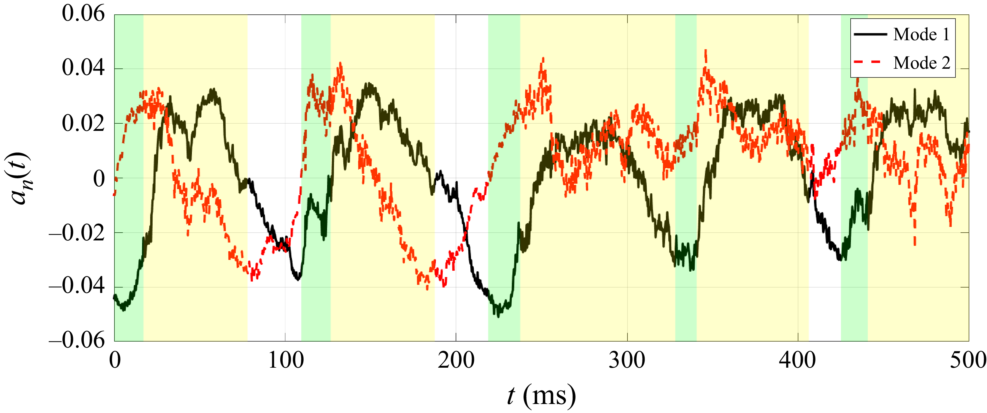
Evolution of the time coefficient ( $a_{n}(t)$ ) for modes 1 and 2 in the upstream domain. The green and yellow regions correspond to growth and collapse phases, respectively.

The evolution of time coefficients for both modes is provided in figure 13, which exhibits strong periodicity. The oscillation frequency of mode 1 is approximately 10 Hz. The behaviour resembles that of the oscillation process of cavitation, indicating their strong correlation. As the sheet and tip vortex cavities grow, the time coefficient becomes positive, reflecting a wall-normal displacement of the vortex. Its magnitude remains nearly constant through the early and middle parts of the collapse stage, before returning to a minimal level once cavitation has fully broken up. For mode 2, the time coefficient undergoes multiple increases and decreases within each cycle during the collapse phase, corresponding to intense deformation of the tip vortex driven by strong spanwise vortices (figure 9 $b$ ). In the rebounding phase, the time coefficient of the deformation mode approaches zero, indicating weak vorticity fluctuations upstream.

3.4.2. Downstream domain

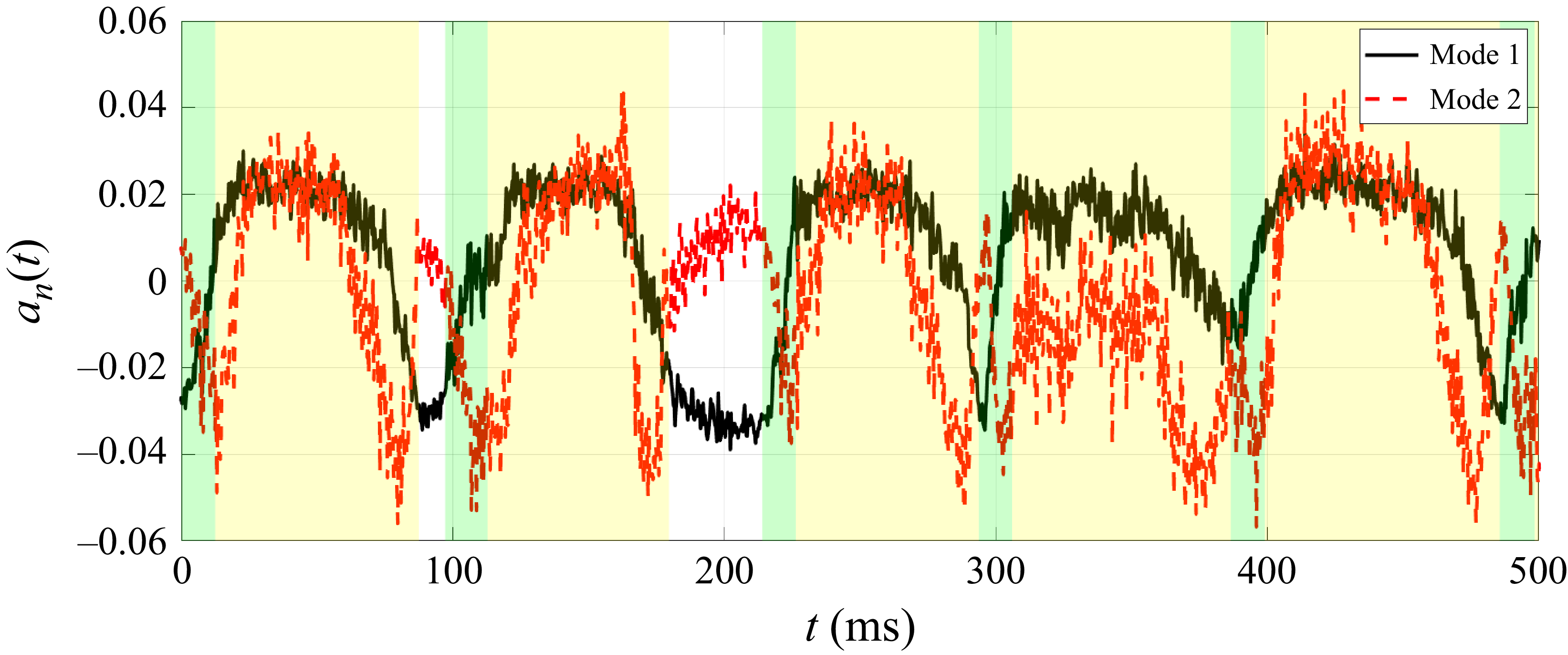
In the downstream domain, modes 1, 2, 6, 8 and 9 are selected. The first two modes with the highest energy represent the vortex centre displacement. The main structure of each mode is a pair of elongated vortex pairs with opposite directions (figures 14 a,b). As shown by the extracted cross-sections (figures 14 c,d), the two displacement modes have a $90^{\circ }$ spatial phase difference, confirming the displacement motion of the tip vortex in all directions. The time coefficient history of the former modes is provided in figure 15, demonstrating clear periodicity following the cavitation cycle. The time coefficients of the two modes also appear in phase quadrature. This behaviour reflects alternating contributions to the wall-normal and spanwise displacement by modes 1 and 2, respectively. The phase difference is related to the anticlockwise rotation of the tip vortex during the cavity growth and collapse process (Vanierschot et al. Reference Toosi, Peplinski, Schlatter and Vinuesa2020).

Figure 14.

Vorticity fluctuation components of POD modes for the temporal and spatial characters of modes in the downstream domain ( $\phi /u_{\infty }=\pm0.017$ ): (a,c) mode 1, (b,d) mode 2. Cross-plane contours are superimposed at $x/c = 0.6$ . The grey iso-surface corresponds to the time-averaged streamwise vorticity.

Figure 15.

Evolution of the time coefficient ( $a_{n}(t)$ ) for modes 1 and 2 in the downstream domain. The green and yellow regions correspond to growth and collapse phases, respectively.

Figure 16.

Vorticity fluctuation components of POD modes for the temporal and spatial characters of modes in the downstream domain ( $\phi /u_{\infty }=\pm0.017$ ): ( $a$ ) mode 6, ( $b$ ) mode 8, ( $c$ ) mode 9. The grey iso-surface corresponds to the time-averaged streamwise vorticity.

Modes 6, 8 and 9 exhibit a different mode pattern, consisting of pairs of anticlockwise spiral vorticity fluctuation pairs (figures 16 $a$ – $c$ ), similar to the helical coherent structures reported for swirling-jet vortex breakdown (Vanierschot et al. Reference Toosi, Peplinski, Schlatter and Vinuesa2020). The streamwise distance between neighbouring spiral pairs is approximately $0.2c$ , which is consistent with the distance between the secondary vortices in figures 9 and 10. Meanwhile, modes 6 and 8 exhibit a streamwise spatial shift of approximately $0.05c$ between their corresponding pairs of vorticity fluctuations, equivalent to one-quarter of the dominant wavelength ( $0.2c$ ), indicating shedding of vorticity that wraps around the tip vortex (Noack et al. Reference Noack, Stankiewicz, Morzyński and Schmid2016). This interpretation agrees with the modal analyses of Wang et al. (Reference Venning, Pearce and Brandner2022), which show that the secondary vortices roll up and organise coherent structures, injecting fluctuations into the tip vortex, thereby amplifying unsteadiness. The evolution of the time coefficient (figure 17) shows high amplitudes during the collapse and rebounding phases, further validating the shedding mechanism of secondary vortices in both phases.

Figure 17.

Evolution of the time coefficient ( $a_{n}(t)$ ) for modes 6, 8, 9 in the downstream domain. The green and yellow regions correspond to growth and collapse phases, respectively.

Figure 18.

Wavelet power spectrum $P_{w} (t, f )$ for time coefficient of modes in the downstream domain: ( $a$ ) mode 1, ( $b$ ) mode 6.

To further examine the dynamic evolution of these modes at different phases, the wavelet transform is employed to analyse unsteady and transient features associated with the growth, collapse and rebounding of cavitation (Brandner, Venning & Pearce Reference Brandner, Venning and Pearce2018). Figure 18 presents the wavelet analysis of the time coefficients of the downstream modes 1 and 6, where $P_{w} (t, f )$ denotes the wavelet power spectrum at time $t$ and frequency $f$ , quantifying the signal energy within the corresponding time–frequency window. The peak frequency of mode 1 is mainly concentrated around 10 Hz (figure 18 $a$ ), which is close to the large-scale cavitation shedding frequency shown in figure 4. Mode 6 shows a second peak frequency within the 100–400 Hz frequency band during the collapse and rebounding phases (figure 18 $b$ ), which is attributed to the spanwise vortex shedding near the tip.

The POD modes show that the unsteady evolution of cavitation induces both displacement and deformation of the tip vortex. In the upstream domain, displacement (mode 1) and deformation (mode 2) both dominate due to strong vortex–vortex interactions, exhibiting frequency approximately 10 Hz, consistent with the cavitation oscillation cycle. In the downstream domain, the vorticity fluctuations are primarily governed by the displacement mode. Modes with higher shedding frequency also emerge, which align with secondary vortices rolling up and wrapping around the tip vortex.

3.5. Turbulence production

The unsteady behaviour of sheet and vortex cavitation drives the collapse of the tip vortex and vortex–vortex interactions, leading to the growth of disturbances in the flow field. To analyse the generation and transport of energy, we calculate the spatial distribution of the turbulence production ( $P_{k}$ ) in the growth, collapse and rebounding phases separately, following

(3.3) \begin{equation} P_k = - \overline {u_i' u_{\!j}'}\, \frac {\partial \overline {u}_i}{\partial x_{\!j}}. \end{equation}

The spatial distribution of the normalised production term ( $P_k^{*}= P_{k}c/u_{\infty }^{3}$ ) is provided in figure 19 for seven $y$ – $z$ cross-sections ( $x/c= -0.1, 0, 0.1, 0.2, 0.4, 0.6, 0.8$ ). The present analysis focuses on the positive component of $P_{k}^{*}$ , which indicates turbulent kinetic energy (TKE) transfer from the mean flow to turbulence (Pope Reference Podbevšek, Petkovšek, Ohl and Dular2001). In all phases, positive $P_{k}^{*}$ emerges at the tip ( $x/c = 0$ ), and concentrates within the surface boundary layer (figures 19 $a$ i $b$ i, $c$ i). Downstream at $x/c = 0.1$ , a large-magnitude band develops and connects to the tip vortex core, indicating that production originates from the suction-side boundary layer where strong shear is present (Li, Chen & Katz Reference Li, Chen and Katz2017), and is transported into the tip vortex. For the growth and collapse phases, the volumetric evolution and break-up of the cavity strongly modulate the production of TKE. A large-magnitude band of positive $P_{k}^{*}$ persists at $x/c = 0.2$ (figures 19 $a$ i, $b$ i), continuing to feed the growth of fluctuation components at the tip vortex core. This aligns with instantaneous fields showing interactions between spanwise vortices and the tip vortex (figures 8 and 9), which drive displacement and deformation of the tip vortex (figure 12). The result is consistent with the previous research, which proposed that the turbulence is generated within the braid structures between interacting vortices and transported into the vortex core (Hussain Reference Hussain1981; Lignarolo et al. Reference Lignarolo, Ragni, Scarano, Simão Ferreira and van Bussel2015). In the rebounding phase, $P_{k}^{*}$ decays rapidly as the tip vortex detaches from the suction side at $x/c = 0.2$ (figure 19 $c$ i). The vortex core exhibits negative $P_{k}^{*}$ , indicating that energy is extracted from the local turbulent fluctuations within the tip vortex and returned to the mean flow, resembling the trend for the wetted flow condition (Zhao et al. Reference Zhang, Zhang, Peng, Wang and Shao2025).

In the downstream region (figures 19 $a$ ii, $b$ ii, $c$ ii), both the growth and collapse phases display alternating positive and negative patches of $P_{k}^{*}$ , indicating that the unsteady evolution of cavitation drives energy exchange between the tip vortex and the mean flow (Liu et al. Reference Liu, Tang, Yan and Li2022). The positive $P_{k}^{*}$ is an extension of the high-magnitude region along the upstream hydrofoil surface, highlighting that vortex–vortex interactions upstream amplify the downstream tip vortex instability. The present result is consistent with the $P_{k}^{*}$ distributions reported by Posa, Broglia & Balaras (Reference Pope2021) for downstream vortex breakdown, where the positive and negative $P_{k}^{*}$ appear around the tip vortex. The rebounding phase exhibits weaker $P_{k}^{*}$ , in line with a relatively stable tip vortex state downstream.

Figure 19.

The spatial distributions of the normalised production term $P_{k}^{*}$ , for $x/c = -0.1, 0, 0.1, 0.2,{} 0.4, 0.6, 0.8$ : ( $a$ ) growth phase (I), ( $b$ ) collapse phase (II), ( $c$ ) rebounding phase (III), for (i) FOV A, (ii) FOV B. The grey iso-surface corresponds to the time-averaged streamwise vorticity for phases I and III, respectively. In phase II, cavitation collapse leads to the absence of the tip vortex in the time-average flow field.

Figure 20.

Integrals of the production terms $\mathrm{\varPi }_{ij}^{*}$ at each streamwise cross-section for three phases: ( $a$ ) I, growth, ( $b$ ) II, collapse, and ( $c$ ) III, rebounding.

Further analysis isolates the contribution of each term in (3.3). The streamwise gradient component is negligible for the present configuration. The contributions of spanwise and wall-normal velocity gradient to the production of TKE are investigated in detail, following

(3.4) \begin{equation} P_{k2} = -\left[ \overline {v' u'}\, \frac {\partial \overline {v}}{\partial x} + \overline {v' v'}\, \frac {\partial \overline {v}}{\partial y} + \overline {v' w'}\, \frac {\partial \overline {v}}{\partial z} \right]\!, \end{equation}

(3.5) \begin{equation} P_{k3} = -\left[ \overline {w' u'}\, \frac {\partial \overline {w}}{\partial x} + \overline {w' v'}\, \frac {\partial \overline {w}}{\partial y} + \overline {w' w'}\, \frac {\partial \overline {w}}{\partial z} \right]\!. \end{equation}

The integrals of (3.4) and (3.5) are calculated for each streamwise section, following

(3.6) \begin{equation} \varPi _{ij} = \iint _{S} -\overline {u_i' u_{\!j}'}\, \frac {\partial \overline {u}_i}{\partial x_{\!j}}\, \text{d}S, \quad \text{with } \quad {-\overline {u_i' u_{\!j}'}}\, \frac {\partial \overline {u}_i}{\partial x_{\!j}} \gt 0 \ (i = 2,3;\ j = 1,2,3), \end{equation}

where $S$ denotes the test region that contains both the tip vortex and spanwise vortices. The streamwise development of the non-dimensional term $\varPi _{ij}^{*} = \varPi _{ij}c/u_{\infty }^{3}$ of each component is illustrated in figure 20. The sum of the six terms ( $\varPi _{2j}^{*}+\varPi _{3j}^{*}$ ) is calculated and shown as the black line with circles. Across all three phases, the sum term increases monotonically from the leading edge, reaches a peak and then decays. In the growth and collapse phases, the peaks occur at $x/c = 0.17, 0.22$ , respectively, coinciding with the locations of pronounced interactions between tip and spanwise vortices in figures 8(b) and 9(b). In the rebounding phase, the decay starts further upstream ( $x/c= 0.11$ ), exhibiting a lower amplitude globally.

Among all the individual components, the dominant term is $\varPi _{22}^{*}$ , which reflects the strong wall-normal strain ( $\partial \overline {v}/\partial y$ ) generated by the rolled-up shear layer, and subsequently feeds the growth disturbances of the tip vortex system, consistent with the previous study (Zhao et al. Reference Zhang, Zhang, Peng, Wang and Shao2025). The spanwise-related terms $\varPi _{32}^{*}$ and $\varPi _{33}^{*}$ also reach comparable levels, indicating spanwise modulation by the suction-side shear layer and its contribution to TKE production (Bilbao-Ludena & Papadakis Reference Bilbao-Ludena and Papadakis2023).

3.6. Noise radiation

The cavitation undergoes significant temporal volume variations, which leads to noise radiation. To analyse the noise magnitude, the recorded voltage was converted to pressure $p_s$ based on the hydrophone sensitivity. Then the sound pressure level (SPL) was calculated, defined as

(3.7) \begin{equation} \mathrm{SPL} = 20 \log _{10}\left (\frac {p_s}{p_{\mathit{ref}}}\right )\!, \end{equation}

where $p_{\mathit{ref}}$ is the reference pressure equal to 1 ${\unicode{x03BC}}$ Pa in the water.

Figure 21 presents the noise spectrum under the fully developed cavitation condition. The wetted flow case is included for reference. In the low-frequency band (below 100 Hz), the noise is primarily attributed to the oscillation cycle of cavitation (figure 4), producing a clear increase in SPL over the wetted flow. In the high-frequency band (250–5000 Hz), a marked broad-band enhancement is observed. This behaviour is consistent with acoustic emissions from the break-up and shedding of cavities and the collapse of microbubbles (Tian et al. Reference Tani, Aktas, Viviani, Yilmaz, Miglianti, Ferrando and Atlar2024).

Figure 21.

The SPLs of the fully developed cavitation ( $\sigma = 4.1$ ) and the wetted flow ( $\sigma = 11.8$ ) conditions.

Figure 22.

Sound pressure signal for one oscillation cycle of the fully developed cavitation (red line) and wetted flow (black line) conditions. The red triangles denote the three time instants in figures 2 and 3, corresponding to the growth ( $t_{\mathrm{2}}$ ), collapse ( $t_{\mathrm{4}}$ ) and rebounding phases ( $t_{\mathrm{7}}$ ).

Figure 22 provides the time series of sound pressure for one oscillation cycle of the fully developed cavitation, compared with the time history of the wetted flow condition. During the oscillation cycle, the primary sources of noise are the rapid volume growth of the sheet and tip vortex cavities, with the highest amplitude approaching 30 Pa, corresponding to the moment when the sheet cavity expands to 80 % of its maximum area ( $t_{\mathrm{2}}$ ). The rapid volume variation rates of cavities generate strong acoustic impulses (Ganesh, Schot & Ceccio Reference Ganesh, Schot and Ceccio2014; Wang, Ye & Shao Reference Wang, Bai, Qian, Cheng and Ji2025). As collapse begins, interfacial fluctuations and break-up of the sheet cavity produce high sound pressure ( $t_{\mathrm{4}}$ ), whereas subsequent shedding of the secondary vortex cavities yields weaker pressure, with its much smaller volumetric variation than in the growth stage. For the rebounding phase, the early rebounding ( $t_{\mathrm{7}}$ ) and contraction of the tip vortex cavity also produce a high sound pressure, followed by a steep magnitude reduction.