2 The Philip Sidney game

The interactions between individuals are modeled by the Philip Sidney game. In biology it is generally accepted as the standard model of costly signaling. The Philip Sidney game, see Figure 1, is a signaling game, introduced by Maynard Smith (Reference Maynard Smith1991). It is a two-player, extensive form game of incomplete information. The first player (Sender) can be in one of two states: healthy or needy, with probability p and 1−p, respectively. In both cases he can either send a signal at some cost c or he can remain silent. Player 2 (Receiver) does not know the true state of Sender, but he can observe whether or not Sender signals. Furthermore, Receiver has a resource and must decide whether or not to donate his resource to Sender.

Figure 1

The Philip Sidney game. Depending on the signal sent by Sender, Receiver is in one of two information states. An information state is a set of player nodes which the player cannot distinguish from each other. Decision nodes which belong to the same information state are connected by a dotted line. The utilities are given at the terminal nodes. The first utility belongs to Sender, the second to Receiver

The players’ chances of survival depend on the state t ∈ {healthy, needy}, the signal s ∈ {signal, silent}, and the action a ∈ {donate, keep} as follows. If Receiver keeps the resource to himself, he is sure to survive. If he donates the resource to Sender his chances of survival v _R(t, s, a) are reduced to S<1, see Equation (1):

(1) $$v_{R} (t,\,s,\,a)=\left(\!\!{\matrix{ S &#x0026; {if\,a=\,donate,} \cr 1 {if\,a=\,keep}}}\!\!\right).$$

On the other hand, Sender is sure to survive if he receives the resource. If Sender does not receive the resource and he is needy, then his chance of survival is 0. If he does not receive the resource and he is healthy, then his chance of survival is V<1. Thus, he benefits more from receiving the resource when he is needy, than when he is healthy. The survival probabilities for Sender v _S(t, s, a) for state t, signal s, and action a are summarized by Equation (2):

$$v_{S} (t,\,s,\,a)=\left(\!\!{\matrix{ {(1{\minus}c)w_{{t,a}} } &#x0026; {if\,s=signal,} \cr \hskip-22pt{w_{{t,a}} } &#x0026; {if\,s=silent,}}}\!\!\right).$$

where c is the signal cost and w _t,a an element of matrix w:

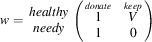$$w= \matrix{ {healthy} \cr {needy} \cr } \,\left( {\matrix{ {\mathop{1}\limits^{{donate}} } &#x0026; {\mathop{V}\limits^{{keep}} } \cr 1 &#x0026; 0 \cr } } \right)$$

Clearly, there is no reason for Receiver to donate his resource, except that the players may be related by some factor r, such that a player also benefits from the survival of the other. This is known as the principle of inclusive fitness (Hamilton, Reference Hamilton1964). The utility u of each player is his survival probability plus a fraction r of the other player’s survival probability. See Equations (3) and (4) for Sender’s and Receiver’s utilities, u _S and u _R, respectively.

(3) $$u_{S} (t,\,s,\,a)=v_{S} (t,\,s,\,a){\plus}rv_{R} (t,\,s,\,a)$$

(4) $$u_{R} (t,\,s,\,a)=v_{R} (t,\,s,\,a){\plus}rv_{S} (t,\,s,\,a)$$

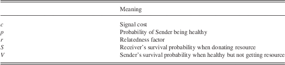
Increasing the relatedness factor r reduces the conflict between the players. When the relatedness factor r=1, both players have the same utilities. The game tree and the utilities for each possible outcome of the Philip Sidney game are shown in Figure 1 and the parameters are summarized in Table 1.

Table 1

Parameters of the Philip Sidney game

Parameters c and r are in the closed interval [0, 1], p, S, and V in the open interval (0, 1).

We now wonder under what circumstances Sender should honestly signal his state (signal when he is needy, and remain silent when he is healthy) and Receiver should trust the Sender (donate when Sender signals, and keep otherwise).

The Philip Sidney game is a good model for the handicap principle since signals can be costly. Moreover, Sender’s benefit of receiving the resource is higher when he is needy than when he is healthy. On the other hand, the cost of signaling does not depend on the state of Sender, but only on the signal intensity. Figure 2 visualizes this assuming there is a continuum of possible signals. This is not the case for the Philip Sidney game, but the reasoning remains the same. In any case, there exists an optimal signal intensity where the benefits maximally outweigh the costs (the vertical lines in Figure 2). Depending on the parameters of the game the optimal signal intensity for needy individuals may be higher than for healthy individuals. This means, that in those cases healthy individuals cannot profit from being dishonest. In other words, honest signaling is a (Nash) equilibrium.

Figure 2

Visual representation of the handicap principle where signal cost and benefits increase with signal intensity. The benefit for a needy individual is higher than for a healthy one such that the optimal signaling intensity is higher for needy individuals

2.1 Evolutionary stability

The handicap principle only indicates there is a possibility that honest signaling is stable. To verify its stability one usually relies on the concept of evolutionarily stable strategies. A strategy is evolutionary stable when an entire population that adopts the strategy, cannot be invaded by a mutant strategy (Maynard Smith and Price, Reference Maynard Smith and Price1973). For honest signaling to be evolutionary stable Sender’s strategy (‘signal only when needy’) must be the best response to Receiver’s strategy (‘donate only when Sender signals’) and also the other way around: Receiver’s strategy (‘donate only when Sender signals’) must be the best response to Sender’s strategy (‘signal only when needy’).

Straightforward algebra shows that ‘signal only when needy’ is a best response to ‘donate only when Sender signals’ whenever r<1−c+rS and 1−c+rS<V+r. Similarly, ‘donate only when Sender signals’ is a best response to ‘signal only when needy’ whenever 1+rV>S+r and S+r(1−c)>1 (Maynard Smith, Reference Maynard Smith1991). Note that the probability p of Sender being healthy does not influence the evolutionary stability. For the Philip Sidney games where S=V=0.8, Figure 3(a) shows for which combinations of signal cost c and relatedness factor r honest signaling is evolutionary stable.

Figure 3

(a) Stability of honest signaling and (b) conflict for all combinations of signal cost c and relatedness factor r, and parameters S=V=0.8. The figures are independent of the probability of Sender being healthy (p)

The Philip Sidney game is an asymmetric two-player game since the players have different roles (Sender and Receiver) and for every asymmetric two-player game the set of evolutionarily stable strategies is equal to the set of strict Nash equilibria (Fudenberg and Levine, Reference Fudenberg and Levine1998) and hence, we may interchange both terms. Remember that a Nash equilibrium is a set of strategies, one for each player, such that none of the players can be better off by unilaterally deviating from the equilibrium and a strict Nash equilibrium is a set of strategies, one for each player, such that none of the players can be strictly better off by unilaterally deviating from the equilibrium. For honest signaling to be a strict Nash equilibrium, again, Sender’s strategy (‘signal only when needy’) must be the best response to Receiver’s strategy (‘donate only when Sender signals’) and Receiver’s strategy must be the best response to Sender’s strategy.

2.2 Conflict and costly signals

Remember that we try to understand under which circumstances signaling between individuals with conflicting interests will be honest. It is informative to verify when there is a conflict. We say there is a conflict of interest between the two players when there exists a state t ∈ {healthy, needy} such that for all signals s ∈ {signal, silent} the players prefer different actions a, b ∈ {donate, keep} (Maynard Smith, Reference Maynard Smith1991). More formally there is a conflict of interest if and only if

(5) $$\exists \,t,\forall \,s\,\,\colon\,\,{\rm arg}\,\:{\rm max}_{a} \,u_{S} (t,\,s,\,a)\,\,\ne\,\,{\rm arg}\,\:{\rm max}_{b} \,u_{R} (t,\,s,\,b)$$

where u _S(t, s, a) and u _R(t, s, a) are Sender’s and Receiver’s utility for outcome with state t, signal s, and action a, respectively. If Equation (5) holds for all states t, we say there is a full conflict, if it holds for none, we say there is no conflict, and otherwise we say there is a partial conflict.

Concretely, there is a conflict when Sender is healthy if r(1−V)<1−S and r(1−S)<(1−c)(1−V). Similarly, there is a conflict when Sender is needy if r<1−S and r(1−S)<(1−c). Note that the existence of conflict does not depend on the probability of Sender being healthy or needy. Figure 3(b) shows the different regions of conflict for all combinations of signal cost c and relatedness factor r when the parameters S=V=0.8. Maynard Smith (Reference Maynard Smith1991) showed furthermore that if there is no signal cost (c=0), honest signaling can only be stable if there is no conflict. When there is a conflict, honest signaling can only be stable if signals are costly (c>0). The latter is the handicap principle. Note that honest signaling cannot be stable if there is a full conflict. If Sender would truthfully reveal his state, Receiver would do exactly the opposite of what Sender prefers.

Knowing whether or not there is a conflict may help in predicting the outcome of the game. When there is a full conflict, we may expect to see ‘never signal, never donate’. When there is no conflict, we may expect to see ‘never signal, always donate’. Both cases are states of no communication. We will see that this intuition is correct (Section 4).

3 Selfish adaptive behavior

Reinforcement learning algorithms are ideal as models of simple adaptive behavior of selfish individuals. A reinforcement learner repeatedly observes the state of the environment, selects an action and receives a payoff indicating the quality of his action. An individual can maintain statistics of the payoffs for all combinations of observations and actions. This way, he can learn which are the most rewarding actions in each state of the environment and hence change his behavior by selecting better actions more often.

We use Q-learning (Watkins & Dayan, Reference Watkins and Dayan1992) with ε-greedy action selection, because of its ease of applicability. The parameters are easy to tune and the algorithm poses no constraints on the payoffs. Sender has a Q-value Q _t,s for each possible state t ∈ {healthy, needy} and each possible signal he can send, s ∈ {signal, silent}. Receiver has a Q-value Q _s,a for each possible signal he can observe, s ∈ {signal, silent}, and each possible action he can take, a ∈ {donate, keep}.

We initialize Q-values optimistically by setting them to a value which is greater than or equal to the highest payoff of the game. This makes sure that there is sufficient exploration in the beginning of the game (Sutton & Barto, Reference Sutton and Barto1998: 40). In the experiments we set initial Q-values to 2.

Now, for each game with outcome (t, s, a), both players update the Q-value that corresponds to the observation they made and the action they took during that game, according to the update rule (6). The other Q-values remain unchanged

(6) $$\matrix{ {Q_{{t,s}} \,} {\leftarrow Q_{{t,s}} \,{\plus}\,\alpha \,\left( {u_{S} (t,\,s,\,a)\,{\minus}\,Q_{{t,s}} } \right)} \hfill \cr {Q_{{s,a}} } \,{\leftarrow Q_{{s,a}} \,{\plus}\,\alpha \,\left( {u_{R} (t,\,s,\,a)\,{\minus}\,Q_{{s,a}} } \right)} \hfill \cr } $$

In this update rule, α ∈ [0, 1] represents the learning rate. In the extreme case of α=0, nothing is ever learned. In the other extreme case where α=1, Q-values only reflect the last reward for the corresponding action. In fact, the Q-values represent the exponentially weighted moving average of the utilities (Sutton & Barto, Reference Sutton and Barto1998: 38). Both players used the same learning rate α=0.1 in all experiments.

To balance exploration and exploitation, we used ε-greedy action selection: with probability 1−ε individuals select the action with the highest Q-value (braking ties randomly) and with probability ε they select an action at random according to a uniform distribution. For all experiments we used a constant exploration rate ε=0.01.

Note, that we use the so-called ‘single-state’ Q-learning. The reason for this is that each player only reaches one information state per game and takes only one action. Hence, there can be no information transfer between information states. Remember that Sender has information states healthy and needy, Receiver has information states signal and silent, and that per game the state can be either healthy or needy. In both cases Sender will either signal or remain silent.

One can prove that Q-learning will find the optimal policy, that is, the Q-values converge to the true total expected utility provided that the environment is stationary and actions are selected infinitely often (Watkins & Dayan, Reference Watkins and Dayan1992). Unfortunately, in a multi-agent setting the environment is non-stationary due to the presence of other agents who also learn and hence change their behavior. Whereas in a stationary environment exploration can be ignored once enough information has been collected, in a non-stationary environment the agent has to continue exploring in order to track changes in the environment. That is also why we used a constant exploration rate ε.

4 Experiments and results

In all experiments reported here, initial Q-values were 2, the learning rate α=0.1, and the exploration rate ε=0.01 for all players. The population consisted of 100 individuals. We repeatedly selected two individuals at random to play a game. On average each individual was selected 10 000 times as Sender and 10 000 times as Receiver. During each simulation we recorded the outcomes of each game. An outcome consists of a state t ∈ {healthy, needy}, a signal s ∈ {signal, silent}, and an action a ∈ {donate, keep}. To get an accurate estimate of the probability of seeing a specific outcome at any timestep we used a moving average. Finally, the results were averaged over 100 simulations/experiment. An example of an experiment is shown in Figure 4 for signal cost c=0.1, relatedness factor r=0.25, S=V=0.8, and p=0.5. It shows the evolution of the frequencies of each of the outcomes over time.

Figure 4

A typical experiment for the Philip Sidney game with parameters S=V=0.8, p=0.5, c=0.1, and r=0.25. The figure shows the evolution of the frequencies of each of the outcomes over time. Each outcome can occur at most half of the time, since the state t ∈ {healthy, needy} is included in the outcome and the probability distribution over the states is fixed at (p, 1−p). In this case, when Sender is needy he almost always signals and Receiver mostly donates (this outcome is abbreviated by ‘nsd’). When Sender is healthy, about half of the time he remains silent and Receiver keeps the resource (‘hlk’), and about half the time Sender bluffs and gets the resource (‘hsd’)

In Figure 5, we show for which combinations of signal cost c and relatedness factor r honest signaling evolves. Honest signaling is the strategy pair ‘signal only when needy, donate only when signal’, so the frequency of honest signaling is the sum of the frequencies of the outcomes (healthy, silent, keep) and (needy, signal, donate). In particular, dark red in the figure indicates honest signaling was always observed, dark blue indicates that honest signaling was never observed.

Figure 5

Frequency of honest signaling for all combinations of signal cost c and relatedness factor r. The other parameters of the Philip Sidney game are S=V=0.8 and p=0.5

Three things are remarkable:

• ∙ First, it is particularly surprising that in a large part of the area where honest signaling is evolutionary stable (the area enclosed by the points (0, 1), (0.8, 1), and (0.153, 0.236)), honest signaling does not evolve! It only does so near the lower tip of that region at (0.153, 0.236).

• ∙ Second, there is a red/orange/yellow region (to the left of the lower tip) where honest signaling is not evolutionary stable, still it evolves.

• ∙ Finally, the green area in the lower part of the figure seems to indicate honest signaling is observed 50% of the time.

Let us now try to explain each of these observations.

When honest signaling is stable: in the region where honest signaling is stable, we only observed honest signaling near the lower tip (Figure 5). The reason why honest signaling not necessarily evolves even though it is an equilibrium lays in the fact that an other equilibrium may dominate honest signaling. In our example (Philip Sidney games with parameters S=V=0.8 and p=0.5) the strategy pair ‘never signal, always donate’ is a Nash equilibrium for many combinations of signal cost c and relatedness r. Even more, for an important set of games where honest signaling is a Nash equilibrium, honest signaling is Pareto-dominated by the Nash equilibrium ‘never signal, always donate’. The frequency at which the strategy pair ‘never signal, always donate’ was observed is shown in Figure 6. Clearly, for many games where honest signaling is a Nash equilibrium ‘never signal, always donate’ was, nevertheless, observed with high frequency (>0.9).

Figure 6

Frequency of the strategy pair ‘never signal, always donate’ for all combinations of signal cost c and relatedness factor r. The other parameters of the Philip Sidney game are S=V=0.8 and p=0.5

Figure 7 shows for which Philip Sidney games honest signaling is Pareto-dominated by another Nash equilibrium. The region where honest signaling is an unique Pareto-optimal Nash equilibrium, is also where we observed honest signaling. The region where honest signaling is a Pareto-optimal Nash equilibrium but not an unique one is where honest signaling sometimes emerged. Finally, we never observed honest signaling in the region where honest signaling is a Nash equilibrium Pareto-dominated by another Nash equilibrium. This also holds for other values of p, the probability of Sender being healthy. Note that, whether or not honest signaling is a Nash equilibrium is independent of the probability p that Sender is healthy (see Section 2.1 and Figure 3(a)), but that Pareto-optimality of equilibria does depend on p.

Figure 7

For which combinations of signal cost c and relatedness factor r honest signaling is a Nash equilibrium of the game. The other parameters of the Philip Sidney games are S=V=0.8 and p=0.5. In the biggest part of that area honest signaling is a Nash equilibrium Pareto-dominated by another equilibrium. In the region below it, it is not Pareto-dominated, but there is an other Nash equilibrium that is also not Pareto-dominated. Finally in the lower tip, honest signaling is an unique Pareto-optimal Nash equilibrium

Clearly, other equilibria may be more important and we need to take this into account in order to predict the outcome of a game. By determining the evolutionary stability of honest signaling alone one overlooks other more important equilibria. One way to determine the importance of equilibria is to see whether or not they are Pareto-optimal. This may clear up some cases, but it is possible that multiple Pareto-optimal Nash equilibria exist in which case multiple equilibria may emerge.

Also note that, for a given signal cost (e.g. c=0.2 in Figure 8), the amount of communication increases if the conflict intensifies (or, in other words, the relatedness factor r decreases) until all communication suddenly stops when relatedness r<1/5(1−c).

Figure 8

Frequency of honest signaling for varying relatedness r for signal cost c=0.2, S=V=0.8, and p=0.5

Partial communication: there are cases where we observed partial communication although honest signaling is not evolutionary stable. The region is more or less located for signal cost c between 0 and 0.15, and relatedness factor r between 0.2 and 0.3 (Figure 5). In this region, it pays Receiver to donate most of the time when Sender signals. Sender is best off by signaling when needy. When healthy, he may sometimes bluff (‘signal when healthy’), but not always. The same region is colored green in Figure 9, indicating that about 50% of the time when Sender is healthy he does not bluff, he remains silent. This is an interesting finding. We observe that being sometimes honest and sometimes dishonest can be an equilibrium where neither full communication (honest signaling), nor no communication is a stable outcome. The experiment shown in Figure 4 is an example of such a case: Sender signals always when needy, and about 50% of the time when healthy. Receiver always keeps when Sender is silent, and donates about 90% of the time.

Figure 9

Frequency of outcome (healthy, silent, keep) for all combinations of signal cost c and relatedness factor r. The other parameters of the Philip Sidney game are S=V=0.8 and p=0.5

Figure 10(a) shows the region where Sender bluffs and Figure 10(b) shows the frequency of bluffing for signal cost c=0.05. For a given signal cost c, intensifying the conflict (by decreasing the relatedness factor r) makes bluffing payoff more and more. When the relatedness factor r is about 0.3 bluffing is near its maximum and decreasing the relatedness factor r even further decreases the equilibrium bluffing rate until the relatedness factor r crosses the curve r=1/5(1−c). At that point, the conflict makes ‘never donate’ a better strategy for Receiver. We find it interesting to see that intensifying a conflict (by decreasing the relatedness r from about 0.3 to 0.2) may decrease the amount of dishonesty and increase the amount of honesty (see Figure 10(b)).

Figure 10

Frequency of bluffing for parameters S=V=0.8 and p=0.5 for (a) varying signal cost c and relatedness r and (b) signal cost c=0.05

For small conflicts (relatedness r>0.4) bluffing does no longer payoff since Receiver is better off by always donating. For extreme conflicts (r<1/5(1−c)) it does not payoff for Sender to bluff for the opposite reason: Receiver is always doing better by keeping the resource anyway. Finally, note that, bluffing almost always payed off. This means that Sender is somehow able to learn an optimal bluffing rate, above which Receiver would no longer trust the signal.

Full conflict: the 50% of honest signaling observed in the Philip Sidney games in the lower part of Figure 5 is entirely due to the outcome (healthy, silent, keep), as is shown in Figure 9. The reason is that, in that region, it does not payoff for Receiver to donate whatever the state of Sender, and consequently, it does not payoff for Sender to signal. Sender will never signal unless the signal cost c is 0. The resulting strategy pair in that region is ‘never signal, never donate’ which partially overlaps with honest signaling (‘signal only when needy, donate only when signal’) but is in fact a state of no communication.

5 Related work

Huttegger and Zollman (Reference Huttegger, Skyrms, Smead and Zollman2010) study evolutionary dynamics in the Philip Sidney game, and contrast their results to those obtained by calculating the evolutionarily stable strategies. They find that in many cases honest signaling has far smaller basins of attraction than other equilibria. This may mean that honest signaling is far less significant as is suggested by the existence of evolutionary stable strategies. Indeed, there is an ongoing debate about how widespread honest signaling really is (Maynard Smith & Harper, Reference Maynard Smith and Harper2003; Searcy & Nowicki, Reference Searcy and Nowicki2005). Our work is exploring the same question and comes to the same conclusion by analyzing dynamics of a learning process.

Another part of the literature is concerned with partially honest signaling. Lachmann and Bergstrom (Reference Lachmann and Bergstrom1998), for example, show the existence of many partial pooling equilibria, where Senders of different but very similar quality use the same signal. Huttegger and Zollman (Reference Huttegger, Skyrms, Smead and Zollman2010) show the existence of mixed equilibria where the Sender is sometimes honest and sometimes dishonest. Here, we found a similar equilibrium that emerged when honest signaling is not evolutionary stable.

Closely related to the emergence of honest signaling is the emergence of signaling itself. The emergence of signaling in a game theoretic setting was first studied by Lewis (Reference Lewis1969). His signaling games represent a communication problem where there is neither cost for signaling, nor conflict. The problem is fully cooperative and the goal for the players is to come up with a convention for the meaning of the signals without any pre-existent means of communication. Recently, both evolutionary dynamics (Hofbauer & Huttegger, Reference Hofbauer and Huttegger2008; Huttegger et al., Reference Huttegger and Zollman2009) and learning dynamics (Argiento et al., Reference Argiento, Pemantle, Skyrms and Volkov2009; Barrett & Zollman, Reference Barrett and Zollman2009; Skyrms, Reference Skyrms2010; Catteeuw et al., Reference Catteeuw and Manderick2011; Catteeuw & Manderick, Reference Catteeuw, De Beule and Manderick2013) received more attention and it was shown that perfect communication can evolve from initially random behavior through simple adaptive processes. While we concentrate on honest signaling in this text, we could indeed observe that initially arbitrary signals can acquire meaning through repeated interaction between learning processes.