2.1 Governing equations

Figure 1(a) shows the physical model to be studied, in which a two-dimensional (2-D) linear disturbance passes through an oblique shock wave. In the 2-D Cartesian coordinate system ( $x^{\ast },y^{\ast }$ ), the undisturbed shock wave is fixed at the $y^{\ast }$ axis and the flow field is divided into two regions. Flow is indicated by subscript 1 before the shock wave and by subscript 2 after it. Superscript $\ast$ represents dimensional variables.

Figure 1.

Sketch maps of (a) the physical model and (b) the shock deformation.

2.1.1 Governing equation of flow before and after an oblique shock wave

In the interaction between disturbances and an oblique shock wave, the viscosity is too weak to be ignored. Hence the flow before and after the shock wave is governed by the inviscid Euler equation

(2.1) $$\begin{eqnarray}\frac{\unicode[STIX]{x2202}\boldsymbol{U}_{p}^{\ast }}{\unicode[STIX]{x2202}t^{\ast }}+\frac{\unicode[STIX]{x2202}\boldsymbol{E}^{\ast }}{\unicode[STIX]{x2202}x^{\ast }}+\frac{\unicode[STIX]{x2202}\boldsymbol{F}^{\ast }}{\unicode[STIX]{x2202}y^{\ast }}=\mathbf{0},\end{eqnarray}$$

where

(2.2a-c ) $$\begin{eqnarray}\boldsymbol{U}_{p}^{\ast }=\left(\begin{array}{@{}c@{}}\unicode[STIX]{x1D70C}^{\ast }\\ \unicode[STIX]{x1D70C}^{\ast }u^{\ast }\\ \unicode[STIX]{x1D70C}^{\ast }v^{\ast }\\ \unicode[STIX]{x1D70C}^{\ast }h^{\ast }-p^{\ast }\end{array}\right),\quad \boldsymbol{E}^{\ast }=\left(\begin{array}{@{}c@{}}\unicode[STIX]{x1D70C}^{\ast }u^{\ast }\\ \unicode[STIX]{x1D70C}^{\ast }u^{\ast }u^{\ast }+p^{\ast }\\ \unicode[STIX]{x1D70C}^{\ast }u^{\ast }v^{\ast }\\ \unicode[STIX]{x1D70C}^{\ast }u^{\ast }h^{\ast }\end{array}\right),\quad \boldsymbol{F}^{\ast }=\left(\begin{array}{@{}c@{}}\unicode[STIX]{x1D70C}^{\ast }v^{\ast }\\ \unicode[STIX]{x1D70C}^{\ast }v^{\ast }u^{\ast }\\ \unicode[STIX]{x1D70C}^{\ast }v^{\ast }v^{\ast }+p^{\ast }\\ \unicode[STIX]{x1D70C}^{\ast }v^{\ast }h^{\ast }\end{array}\right).\end{eqnarray}$$

In these equations, $t^{\ast }$ is the time variable; $\unicode[STIX]{x1D70C}^{\ast }$ , $u^{\ast }$ , $v^{\ast }$ , $p^{\ast }$ denote the density, velocities in the $x^{\ast }$ and $y^{\ast }$ directions, and pressure, respectively; $h^{\ast }=e^{\ast }+(\unicode[STIX]{x1D6FE}p^{\ast }/\unicode[STIX]{x1D70C}^{\ast })/(\unicode[STIX]{x1D6FE}-1)$ is the total enthalpy; $e^{\ast }=(u^{\ast 2}+v^{\ast 2})/2$ is the kinetic energy; $\unicode[STIX]{x1D6FE}$ is the specific heat ratio; $\boldsymbol{U}_{p}^{\ast }$ is the conservative flux; and $\boldsymbol{E}^{\ast }$ and $\boldsymbol{F}^{\ast }$ are the convective fluxes in the $x^{\ast }$ and $y^{\ast }$ directions, respectively.

Supposing that the base flow in the uniform and homogeneous field is steady, the base flow $\boldsymbol{U}_{0}^{\ast }=[\unicode[STIX]{x1D70C}_{0}^{\ast },u_{0}^{\ast },v_{0}^{\ast },p_{0}^{\ast }]^{\text{T}}$ is governed by (2.1) but is independent of the coordinates $(x^{\ast },y^{\ast })$ and time $t^{\ast }$ , where the subscript $0$ represents the undisturbed base flow. As shown in figure 1(a), when the incoming base flow with the velocity vector $\boldsymbol{v}_{01}^{\ast }=(u_{01}^{\ast },v_{01}^{\ast })$ passes through an oblique shock wave, it yields the base flow with the velocity vector $\boldsymbol{v}_{02}^{\ast }=(u_{02}^{\ast },v_{02}^{\ast })$ after the shock wave. Different from the normal shock wave, which is perpendicular to the direction of the incoming base flow, there is a shock wave angle between the oblique shock wave and the incoming base flow, which is defined as $\unicode[STIX]{x1D6FD}_{1}\subset (0,\unicode[STIX]{x03C0})$ . Notably, an oblique shock wave returns to a normal shock wave when $\unicode[STIX]{x1D6FD}_{1}=\unicode[STIX]{x03C0}/2$ . Because of the inclination characteristic, the flow will be deflected by an oblique shock wave, leading to an angle $\unicode[STIX]{x1D6FD}_{2}$ between the oblique shock wave and the base flow after the shock wave.

A weak disturbance in a free stream can be expressed in the form of a normal mode as

(2.3) $$\begin{eqnarray}\boldsymbol{U}^{\prime \ast }=[\unicode[STIX]{x1D70C}^{\prime \ast },u^{\prime \ast },v^{\prime \ast },p^{\prime \ast }]^{\text{T}}=\hat{a}\boldsymbol{C}^{\ast }\exp (-\unicode[STIX]{x1D6FC}_{d}^{\ast }x^{\ast })\exp (\text{i}\unicode[STIX]{x1D6E9}^{\ast })+\text{c.c.},\end{eqnarray}$$

where

(2.4a,b ) $$\begin{eqnarray}\unicode[STIX]{x1D6E9}^{\ast }=\unicode[STIX]{x1D6FC}_{x}^{\ast }x^{\ast }+\unicode[STIX]{x1D6FC}_{y}^{\ast }y^{\ast }-\unicode[STIX]{x1D714}^{\ast }t^{\ast },\quad \boldsymbol{C}^{\ast }=[\hat{\unicode[STIX]{x1D70C}}^{\ast },\hat{u} ^{\ast },\hat{v}^{\ast },\hat{p}^{\ast }]^{\text{T}}.\end{eqnarray}$$

Here $\unicode[STIX]{x1D736}^{\ast }=(\unicode[STIX]{x1D6FC}_{x}^{\ast },\unicode[STIX]{x1D6FC}_{y}^{\ast })$ , $\unicode[STIX]{x1D714}^{\ast }$ and $\hat{a}$ denote the wavenumber vector, circle frequency and amplitude of the disturbance, respectively; $\unicode[STIX]{x1D6FC}_{d}^{\ast }$ is the decay rate of the amplitude satisfying $\unicode[STIX]{x1D6FC}_{d}^{\ast }\geqslant 0$ ; $\unicode[STIX]{x1D6E9}^{\ast }$ and $\boldsymbol{C}^{\ast }$ are the phase and shape function of the perturbation; and $\text{c.c.}$ stands for complex conjugate.

Unlike the classical normal mode (Reshotko Reference Reshotko1976) in which the wavenumber vector $\unicode[STIX]{x1D736}^{\ast }$ can be a complex number and its imaginary component can describe the variation in amplitude, the wavenumber vector $\unicode[STIX]{x1D736}^{\ast }=(\unicode[STIX]{x1D6FC}_{x}^{\ast },\unicode[STIX]{x1D6FC}_{y}^{\ast })$ in (2.3) is a real number, and a new real parameter $\unicode[STIX]{x1D6FC}_{d}^{\ast }$ is introduced to describe the variation in amplitude, through which the damped wave concept can be introduced clearly.

When the base flow $\boldsymbol{U}_{0}^{\ast }$ is perturbed by a small-amplitude disturbance $\boldsymbol{U}^{\prime \ast }$ , the total flow is $\boldsymbol{U}^{\ast }=\boldsymbol{U}_{0}^{\ast }+\boldsymbol{U}^{\prime \ast }$ . Both the base flow and the total flow satisfy the inviscid Euler equation. Applying the total flow to the governing equation and linearizing with the base flow, one can obtain the linearized disturbance equation governing the disturbance $\boldsymbol{U}^{\prime \ast }$ , which can be written in the following form:

(2.5) $$\begin{eqnarray}\unicode[STIX]{x1D6E4}(\unicode[STIX]{x1D6FC}_{x}^{\ast },\unicode[STIX]{x1D6FC}_{y}^{\ast },\unicode[STIX]{x1D714}^{\ast },\unicode[STIX]{x1D6FC}_{d}^{\ast };\boldsymbol{U}_{0}^{\ast })\boldsymbol{C}^{\ast }=\mathbf{0}.\end{eqnarray}$$

Here $\unicode[STIX]{x1D6E4}$ is an operator through which the wave parameters $\unicode[STIX]{x1D6FC}_{x}^{\ast }$ , $\unicode[STIX]{x1D6FC}_{y}^{\ast }$ , $\unicode[STIX]{x1D714}^{\ast }$ , $\unicode[STIX]{x1D6FC}_{d}^{\ast }$ and the shape function $\boldsymbol{C}^{\ast }$ are determined for a given base flow $\boldsymbol{U}_{0}^{\ast }$ .

Typically there are four types of small disturbance in (2.5): fast acoustic wave, slow acoustic wave, entropy wave and vorticity wave. Any type of disturbance striking a shock wave may generate all four types of wave behind the shock wave. However, as mentioned later, we find that another type of wave can be stimulated behind the shock wave by an incident wave under a certain condition. It is called a damped wave because its amplitude decays along the propagation direction. As shown in figure 1(a), the vector $\unicode[STIX]{x1D736}_{i}^{\ast }$ with wave angle $\unicode[STIX]{x1D703}_{i}$ is an arbitrary incident wavevector before or after the shock wave, while the vectors $\unicode[STIX]{x1D736}_{f2}^{\ast }$ , $\unicode[STIX]{x1D736}_{s2}^{\ast }$ , $\unicode[STIX]{x1D736}_{e2}^{\ast }$ , $\unicode[STIX]{x1D736}_{v2}^{\ast }$ and $\unicode[STIX]{x1D736}_{d2}^{\ast }$ are the stimulated wavevectors of the fast acoustic wave, slow acoustic wave, entropy wave, vorticity wave and damped wave behind the shock wave, respectively, whose corresponding wave angles are $\unicode[STIX]{x1D703}_{f2}$ , $\unicode[STIX]{x1D703}_{s2}$ , $\unicode[STIX]{x1D703}_{e2}$ , $\unicode[STIX]{x1D703}_{v2}$ and $\unicode[STIX]{x1D703}_{d2}$ .

2.1.2 Governing equation of base flow across an oblique shock wave

The condition that must be satisfied across a discontinuity is that the normal mass flux, momentum and energy are all continuous. Thus, the so-called Rankine–Hugoniot (RH) condition (McKenzie & Westphal Reference McKenzie and Westphal1968) can be written as

(2.6) $$\begin{eqnarray}\boldsymbol{E}_{1}^{\ast }(\unicode[STIX]{x1D70C}^{\ast },u^{\ast },v^{\ast },p^{\ast })|_{x_{s}^{\ast }}=\boldsymbol{E}_{2}^{\ast }(\unicode[STIX]{x1D70C}^{\ast },u^{\ast },v^{\ast },p^{\ast })|_{x_{s}^{\ast }},\end{eqnarray}$$

where $x_{s}^{\ast }$ is the location of the shock wave, $\boldsymbol{E}^{\ast }$ is the convective flux in the $x^{\ast }$ direction, and $u^{\ast }$ and $v^{\ast }$ are the velocities perpendicular and parallel to the shock wave, respectively. If the unperturbed discontinuity is an oblique shock wave located at $x_{s}^{\ast }=0$ , the unperturbed base flow on either side of the shock wave satisfies the RH condition, namely

(2.7) $$\begin{eqnarray}\boldsymbol{E}_{1}^{\ast }(\unicode[STIX]{x1D70C}_{01}^{\ast },u_{01}^{\ast },v_{01}^{\ast },p_{01}^{\ast })|_{x_{s}^{\ast }=0}=\boldsymbol{E}_{2}^{\ast }(\unicode[STIX]{x1D70C}_{02}^{\ast },u_{02}^{\ast },v_{02}^{\ast },p_{02}^{\ast })|_{x_{s}^{\ast }=0}.\end{eqnarray}$$

2.1.3 Governing equation of disturbance across an oblique shock wave

For a steady oblique shock, it is necessary to consider the shock deformation caused by a small inlet disturbance when studying the interaction between the disturbance and the shock wave, as shown in figure 1(b). Supposing that an oblique shock wave is located in the plane $x_{s}^{\ast }=0$ , the deformation of the shock wave may be written as

(2.8) $$\begin{eqnarray}x^{\ast }=\,f^{\prime \ast }(y^{\ast },t^{\ast }),\quad \text{where }f^{\prime \ast }\ll 1,\end{eqnarray}$$

through which the velocity vector $\boldsymbol{u}_{d}^{\prime \ast }$ of the distorted shock wave and the velocity vector $\boldsymbol{u}_{r}^{\ast }$ of the fluid relative to the shock wave can be given by

(2.9a,b ) $$\begin{eqnarray}\boldsymbol{u}_{d}^{\prime \ast }=\left(\frac{\unicode[STIX]{x2202}f^{\prime \ast }}{\unicode[STIX]{x2202}t^{\ast }}+\frac{\unicode[STIX]{x2202}f^{\prime \ast }}{\unicode[STIX]{x2202}y^{\ast }}\frac{\text{d}y^{\ast }}{\text{d}t^{\ast }},\frac{\text{d}y^{\ast }}{\text{d}t^{\ast }}\right),\quad \boldsymbol{u}_{r}^{\ast }=\boldsymbol{u}_{0}^{\ast }+\boldsymbol{u}^{\prime \ast }-\boldsymbol{u}_{d}^{\prime \ast }.\end{eqnarray}$$

When the incident perturbation is a plane harmonic wave of the form $\exp (\text{i}\unicode[STIX]{x1D6E9}^{\ast })$ , one can take the deformation $f^{\prime \ast }$ to be of the same form (McKenzie & Westphal Reference McKenzie and Westphal1968):

(2.10) $$\begin{eqnarray}f^{\prime \ast }(y^{\ast },t^{\ast })=\,\hat{f}^{\ast }\exp (\text{i}\unicode[STIX]{x1D6F9}^{\ast })+\text{c.c.},\quad \text{with }\unicode[STIX]{x1D6F9}^{\ast }=\unicode[STIX]{x1D6FC}_{y}^{\ast }y^{\ast }-\unicode[STIX]{x1D714}^{\ast }t^{\ast },\end{eqnarray}$$

where $\hat{f}^{\ast }$ is the amplitude of the shock distortion, which is to be determined from the boundary conditions. Then, the velocity components of the fluid relative to the shock wave are

(2.11a,b ) $$\begin{eqnarray}u_{r}^{\ast }=\boldsymbol{u}_{r}^{\ast }\boldsymbol{\cdot }\boldsymbol{n}_{N}=u_{0}^{\ast }+u^{\prime \ast }+v_{0}^{\ast }\frac{\unicode[STIX]{x1D6FC}_{y}^{\ast }}{\unicode[STIX]{x1D714}^{\ast }}u_{d}^{\prime \ast }-u_{d}^{\prime \ast },\quad v_{r}^{\ast }=\boldsymbol{u}_{r}^{\ast }\boldsymbol{\cdot }\boldsymbol{n}_{T}=v_{0}^{\ast }+v^{\prime \ast }-u_{0}^{\ast }\frac{\unicode[STIX]{x1D6FC}_{y}^{\ast }}{\unicode[STIX]{x1D714}^{\ast }}u_{d}^{\prime \ast }-\frac{\text{d}y^{\ast }}{\text{d}t^{\ast }},\end{eqnarray}$$

where

(2.12a-c ) $$\begin{eqnarray}u_{d}^{\prime \ast }=\frac{\unicode[STIX]{x2202}f^{\prime \ast }}{\unicode[STIX]{x2202}t^{\ast }}=\hat{u} _{d}^{\ast }\exp (\text{i}\unicode[STIX]{x1D6F9}^{\ast })+\text{c.c.},\quad \boldsymbol{n}_{N}\approx \left(1,-\frac{\unicode[STIX]{x2202}f^{\prime \ast }}{\unicode[STIX]{x2202}y^{\ast }}\right),\quad \boldsymbol{n}_{T}\approx \left(\frac{\unicode[STIX]{x2202}f^{\prime \ast }}{\unicode[STIX]{x2202}y^{\ast }},1\right),\end{eqnarray}$$

in which $u_{d}^{\prime \ast }$ is the $x^{\ast }$ component of $\boldsymbol{u}_{d}^{\prime \ast }$ , $\hat{u} _{d}^{\ast }$ is its amplitude, and $\boldsymbol{n}_{N}$ and $\boldsymbol{n}_{T}$ are unit vectors normal and tangential to the deformed shock wave, respectively.

Since the incident plane wave has a small amplitude, in the linear approximation, the perturbed flow on either side of the shock wave also satisfies the RH condition, namely

(2.13) $$\begin{eqnarray}\boldsymbol{E}_{1}^{\ast }(\unicode[STIX]{x1D70C}_{1}^{\ast },u_{r1}^{\ast },v_{r1}^{\ast },p_{1}^{\ast })|_{x_{s}^{\ast }=f^{\prime \ast }}=\boldsymbol{E}_{2}^{\ast }(\unicode[STIX]{x1D70C}_{2}^{\ast },u_{r2}^{\ast },v_{r2}^{\ast },p_{2}^{\ast })|_{x_{s}^{\ast }=f^{\prime \ast }},\end{eqnarray}$$

where $\unicode[STIX]{x1D70C}^{\ast }=\unicode[STIX]{x1D70C}_{0}^{\ast }+\unicode[STIX]{x1D70C}^{\prime \ast }$ and $p^{\ast }=p_{0}^{\ast }+p^{\prime \ast }$ are the density and pressure of the disturbed flow, and $\boldsymbol{v}_{r}^{\ast }=(u_{r}^{\ast },v_{r}^{\ast })$ is a velocity vector of the fluid relative to the shock wave. Furthermore, the frequency $\unicode[STIX]{x1D714}^{\ast }$ and the $y^{\ast }$ component of the wavevector $\unicode[STIX]{x1D736}^{\ast }$ will be continuous, namely

(2.14a,b ) $$\begin{eqnarray}\unicode[STIX]{x1D714}_{1}^{\ast }=\unicode[STIX]{x1D714}_{2}^{\ast },\quad \unicode[STIX]{x1D6FC}_{y1}^{\ast }=\unicode[STIX]{x1D6FC}_{y2}^{\ast }.\end{eqnarray}$$

Linearizing the RH condition of disturbed flow about the unperturbed flow in (2.13) at $x_{s}^{\ast }=0$ , one can obtain the linear RH condition governing the perturbation $\boldsymbol{U}^{\prime \ast }$ . For the ensuing analysis, it is convenient to cast it into the matrix form:

(2.15) $$\begin{eqnarray}\unicode[STIX]{x1D63C}_{1}^{\ast }(\boldsymbol{U}_{1}^{\prime \ast }-\boldsymbol{C}_{b1}^{\ast }u_{d}^{\prime \ast })|_{x_{s}^{\ast }=0}=\unicode[STIX]{x1D63C}_{2}^{\ast }(\boldsymbol{U}_{2}^{\prime \ast }-\boldsymbol{C}_{b2}^{\ast }u_{d}^{\prime \ast })|_{x_{s}^{\ast }=0},\end{eqnarray}$$

where the coefficients $\unicode[STIX]{x1D63C}^{\ast }$ and $\boldsymbol{C}_{b}^{\ast }$ can be found in appendix A.

2.2 Plane wave in a uniform and homogeneous field

For convenience, the flow variables before and after an oblique shock wave are non-dimensionalized by the steady-state free-stream conditions before and after the shock wave, respectively. Namely, the reference parameters before the shock wave are $\unicode[STIX]{x1D70C}_{01}^{\ast }$ , $u_{01}^{\ast }$ and $d^{\ast }$ , and those after the shock wave are $\unicode[STIX]{x1D70C}_{02}^{\ast }$ , $u_{02}^{\ast }$ and $d^{\ast }$ . Here, we use the same reference length $d^{\ast }$ . So the non-dimensional variables of the undisturbed base flow are

(2.16) $$\begin{eqnarray}\boldsymbol{U}_{0}=[\unicode[STIX]{x1D70C}_{0},u_{0},v_{0},p_{0}]^{\text{T}}=\left[1,1,\frac{\cos \unicode[STIX]{x1D6FD}}{\sin \unicode[STIX]{x1D6FD}},\frac{1}{\unicode[STIX]{x1D6FE}M_{n}^{2}}\right]^{\text{T}},\end{eqnarray}$$

where $M_{n}=M\sin \unicode[STIX]{x1D6FD}$ is the normal Mach number defined by the velocity perpendicular to the shock wave, $M=\sqrt{u_{0}^{\ast 2}+v_{0}^{\ast 2}}/c_{0}^{\ast }$ is the Mach number of free-stream flow, $\unicode[STIX]{x1D6FD}$ is the shock wave angle and $c_{0}^{\ast }=\sqrt{\unicode[STIX]{x1D6FE}p_{0}^{\ast }/\unicode[STIX]{x1D70C}_{0}^{\ast }}$ is the speed of sound.

Based on (2.5), the non-dimensional linearized disturbance equation can be written in the matrix form

(2.17) $$\begin{eqnarray}\left[\begin{array}{@{}cccc@{}}\unicode[STIX]{x1D712} & \unicode[STIX]{x1D6FC}_{x}+\text{i}\unicode[STIX]{x1D6FC}_{d} & \unicode[STIX]{x1D6FC}_{y} & 0\\ 0 & \unicode[STIX]{x1D712} & 0 & \unicode[STIX]{x1D6FC}_{x}+\text{i}\unicode[STIX]{x1D6FC}_{d}\\ 0 & 0 & \unicode[STIX]{x1D712} & \unicode[STIX]{x1D6FC}_{y}\\ 0 & (\unicode[STIX]{x1D6FC}_{x}+\text{i}\unicode[STIX]{x1D6FC}_{d})/M_{n}^{2} & \unicode[STIX]{x1D6FC}_{y}/M_{n}^{2} & \unicode[STIX]{x1D712}\end{array}\right]\left[\begin{array}{@{}c@{}}\hat{\unicode[STIX]{x1D70C}}\\ \hat{u} \\ \hat{v}\\ \hat{p}\end{array}\right]=\left[\begin{array}{@{}c@{}}0\\ 0\\ 0\\ 0\end{array}\right],\end{eqnarray}$$

whose dispersion relationship satisfies

(2.18) $$\begin{eqnarray}\unicode[STIX]{x1D712}^{2}\left[\unicode[STIX]{x1D712}^{2}-\frac{(\unicode[STIX]{x1D6FC}_{x}+\text{i}\unicode[STIX]{x1D6FC}_{d})^{2}+\unicode[STIX]{x1D6FC}_{y}^{2}}{M_{n}^{2}}\right]=0,\end{eqnarray}$$

where we have put

(2.19) $$\begin{eqnarray}\unicode[STIX]{x1D712}=\unicode[STIX]{x1D6FC}_{x}+\text{i}\unicode[STIX]{x1D6FC}_{d}+v_{0}\unicode[STIX]{x1D6FC}_{y}-\unicode[STIX]{x1D714}.\end{eqnarray}$$

When the decay rate of the amplitude is zero, namely, $\unicode[STIX]{x1D6FC}_{d}=0$ , solving the above dispersion relation (2.18), one can obtain typical solutions for the fast acoustic wave, slow acoustic wave, entropy wave and vorticity wave written in the united form as

(2.20) $$\begin{eqnarray}\unicode[STIX]{x1D714}=\left(\sin (\unicode[STIX]{x1D703}+\unicode[STIX]{x1D6FD})+\frac{\unicode[STIX]{x1D70E}}{M}\right)\frac{\unicode[STIX]{x1D6FC}}{\sin \unicode[STIX]{x1D6FD}},\quad \text{where }\unicode[STIX]{x1D70E}=\left\{\begin{array}{@{}rl@{}}1, & \quad \text{fast acoustic wave},\\ 0, & \quad \text{entropy{-}vorticity wave},\\ -1, & \quad \text{slow acoustic wave},\end{array}\right.\end{eqnarray}$$

where $\unicode[STIX]{x1D703}\subseteq [-\unicode[STIX]{x03C0},\unicode[STIX]{x03C0})$ is the wave angle and 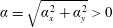$\unicode[STIX]{x1D6FC}=\sqrt{\unicode[STIX]{x1D6FC}_{x}^{2}+\unicode[STIX]{x1D6FC}_{y}^{2}}>0$ is the wavenumber, with $\unicode[STIX]{x1D6FC}_{x}=\unicode[STIX]{x1D6FC}\cos \unicode[STIX]{x1D703}$ and $\unicode[STIX]{x1D6FC}_{y}=\unicode[STIX]{x1D6FC}\sin \unicode[STIX]{x1D703}$ the components of wavenumber vector $\unicode[STIX]{x1D736}$ in the $x$ and $y$ directions, respectively.

When the amplitude decay rate is greater than zero, namely, $\unicode[STIX]{x1D6FC}_{d}>0$ , solving the dispersion relation (2.18), one can obtain the special solution for a damped wave:

(2.21a,b ) $$\begin{eqnarray}\unicode[STIX]{x1D714}=\frac{M_{n}^{2}-1}{M_{n}^{2}}\unicode[STIX]{x1D6FC}_{x}+v_{0}\unicode[STIX]{x1D6FC}_{y},\quad \unicode[STIX]{x1D6FC}_{d}=\sqrt{\frac{\unicode[STIX]{x1D6FC}_{y}^{2}}{1-M_{n}^{2}}-\frac{\unicode[STIX]{x1D6FC}_{x}^{2}}{M_{n}^{2}}},\end{eqnarray}$$

under the condition

(2.22) $$\begin{eqnarray}\frac{\unicode[STIX]{x1D6FC}_{y}^{2}}{1-M_{n}^{2}}>\frac{\unicode[STIX]{x1D6FC}_{x}^{2}}{M_{n}^{2}},\end{eqnarray}$$

from which it can be seen that a damped wave cannot exist before the shock wave but may appear after it. A damped wave usually cannot be discovered in a uniform and homogeneous field because its amplitude of oscillation decreases along the propagation direction, eventually becoming zero. However, it is an important physical part of post-shock excited waves.

The corresponding eigenvector of the solution in (2.18) for the five types of wave can be written in the united form as

(2.23) $$\begin{eqnarray}\left.\begin{array}{@{}ll@{}}\boldsymbol{C}_{f}=[M_{n}^{2},M_{n}\cos \unicode[STIX]{x1D703}_{f},M_{n}\sin \unicode[STIX]{x1D703}_{f},1]^{\text{T}}, & \quad \text{fast acoustic wave},\\ \boldsymbol{C}_{s}=[M_{n}^{2},-M_{n}\cos \unicode[STIX]{x1D703}_{s},-M_{n}\sin \unicode[STIX]{x1D703}_{s},1]^{\text{T}}, & \quad \text{slow acoustic wave},\\ \boldsymbol{C}_{e}=[1,0,0,0]^{\text{T}}, & \quad \text{entropy wave},\\ \boldsymbol{C}_{v}=[0,-\sin \unicode[STIX]{x1D703}_{v},\cos \unicode[STIX]{x1D703}_{v},0]^{\text{T}}, & \quad \text{vorticity wave},\\ \boldsymbol{C}_{d}=[M_{n}^{2},-M_{n}g_{x},-M_{n}g_{y},1]^{\text{T}}, & \quad \text{damped wave},\end{array}\right\}\end{eqnarray}$$

where 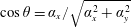$\cos \unicode[STIX]{x1D703}=\unicode[STIX]{x1D6FC}_{x}/\sqrt{\unicode[STIX]{x1D6FC}_{x}^{2}+\unicode[STIX]{x1D6FC}_{y}^{2}}$ , 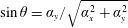$\sin \unicode[STIX]{x1D703}=\unicode[STIX]{x1D6FC}_{y}/\sqrt{\unicode[STIX]{x1D6FC}_{x}^{2}+\unicode[STIX]{x1D6FC}_{y}^{2}}$ , $g_{x}=(\unicode[STIX]{x1D6FC}_{x}+\text{i}\unicode[STIX]{x1D6FC}_{d})/\sqrt{(\unicode[STIX]{x1D6FC}_{x}+\text{i}\unicode[STIX]{x1D6FC}_{d})^{2}+\unicode[STIX]{x1D6FC}_{y}^{2}}$ , $g_{y}=\unicode[STIX]{x1D6FC}_{y}/\sqrt{(\unicode[STIX]{x1D6FC}_{x}+\text{i}\unicode[STIX]{x1D6FC}_{d})^{2}+\unicode[STIX]{x1D6FC}_{y}^{2}}$ , and subscripts $f$ , $s$ , $e$ , $v$ and $d$ represent the fast acoustic wave, slow acoustic wave, entropy wave, vorticity wave and damped wave, respectively. The amplitude of the fast acoustic/slow acoustic/damped wave is defined as the amplitude of the pressure fluctuation, while the amplitudes of the entropy and vorticity waves are defined as the amplitudes of the density and velocity fluctuations, respectively.

The group velocity for four typical types of wave can be written in the united form as

(2.24) $$\begin{eqnarray}\boldsymbol{u}_{g}=(u_{gx},u_{gy})=\left(\frac{\unicode[STIX]{x2202}\unicode[STIX]{x1D714}}{\unicode[STIX]{x2202}\unicode[STIX]{x1D6FC}_{x}},\frac{\unicode[STIX]{x2202}\unicode[STIX]{x1D714}}{\unicode[STIX]{x2202}\unicode[STIX]{x1D6FC}_{y}}\right)=\left(1+\frac{\unicode[STIX]{x1D70E}\cos \unicode[STIX]{x1D703}}{M_{n}},\frac{\cos \unicode[STIX]{x1D6FD}}{\sin \unicode[STIX]{x1D6FD}}+\frac{\unicode[STIX]{x1D70E}\sin \unicode[STIX]{x1D703}}{M_{n}}\right),\end{eqnarray}$$

where the energy of the corresponding wave propagates from upstream to downstream when $u_{gx}>0$ , while the energy of the wave with a negative $u_{gx}$ value propagates from downstream to upstream.

The group velocity for a damped wave is

(2.25) $$\begin{eqnarray}\boldsymbol{u}_{g}=(u_{gx},u_{gy})=\left(\frac{\unicode[STIX]{x2202}\unicode[STIX]{x1D714}}{\unicode[STIX]{x2202}(\unicode[STIX]{x1D6FC}_{x}+\text{i}\unicode[STIX]{x1D6FC}_{d})},\frac{\unicode[STIX]{x2202}\unicode[STIX]{x1D714}}{\unicode[STIX]{x2202}\unicode[STIX]{x1D6FC}_{y}}\right)_{\!r}=\left(1+\frac{\unicode[STIX]{x1D70E}g_{x}}{M_{n}},\frac{\cos \unicode[STIX]{x1D6FD}}{\sin \unicode[STIX]{x1D6FD}}+\frac{\unicode[STIX]{x1D70E}g_{y}}{M_{n}}\right)_{\!r},\end{eqnarray}$$

where subscript $r$ means the real part. It can be proven that $u_{gx}$ is always positive, indicating that the energy of the excited damped wave always propagates downstream when it is excited by an incident plane wave.

2.3 Dispersion relationship of a plane wave across an oblique shock wave

Based on (2.7), it easy to obtain the relationships of the base flow before and after the shock wave, as follows:

(2.26a-c ) $$\begin{eqnarray}v_{01}=u_{b}v_{02},\quad M_{n1}^{2}=\frac{2}{u_{b}(\unicode[STIX]{x1D6FE}+1)-(\unicode[STIX]{x1D6FE}-1)},\quad M_{n2}^{2}=\frac{2u_{b}}{(\unicode[STIX]{x1D6FE}+1)-u_{b}(\unicode[STIX]{x1D6FE}-1)}.\end{eqnarray}$$

Here we prefer to use $u_{b}$ defined as follows to describe the relationship conveniently:

(2.27) $$\begin{eqnarray}u_{b}=\frac{u_{02}^{\ast }}{u_{01}^{\ast }}=\frac{2+(\unicode[STIX]{x1D6FE}-1)M_{n1}^{2}}{(\unicode[STIX]{x1D6FE}+1)M_{n1}^{2}}\in \left(\frac{\unicode[STIX]{x1D6FE}-1}{\unicode[STIX]{x1D6FE}+1},1\right).\end{eqnarray}$$

In order to conveniently study the interaction of plane waves and an oblique shock wave, we define two universal kinds of wavenumber for the excited wave as

(2.28a,b ) $$\begin{eqnarray}\unicode[STIX]{x1D6FC}_{q}\equiv \unicode[STIX]{x1D714}_{2}-v_{02}\unicode[STIX]{x1D6FC}_{y2},\quad \unicode[STIX]{x1D6FC}_{p}\equiv \unicode[STIX]{x1D6FC}_{y2},\end{eqnarray}$$

where $\unicode[STIX]{x1D6FC}_{q}$ is an equivalent wavenumber perpendicular to the surface of the shock wave, while $\unicode[STIX]{x1D6FC}_{p}$ is a wavenumber parallel to it.

Based on (2.14), one can obtain the non-dimensional continuity condition for the frequency $\unicode[STIX]{x1D714}$ and the wavenumber $\unicode[STIX]{x1D6FC}_{y}$ as

(2.29a,b ) $$\begin{eqnarray}\unicode[STIX]{x1D714}_{1}=u_{b}\unicode[STIX]{x1D714}_{2},\quad \unicode[STIX]{x1D6FC}_{y1}=\unicode[STIX]{x1D6FC}_{y2}.\end{eqnarray}$$

Substituting (2.28) and (2.29) into (2.20), one can obtain the following relationship for four classical types of wave before and after the shock wave:

(2.30a,b ) $$\begin{eqnarray}\left(\cos \unicode[STIX]{x1D703}_{1}+\frac{\unicode[STIX]{x1D70E}_{1}}{M_{n1}}\right)\frac{\unicode[STIX]{x1D6FC}_{1}}{u_{b}}=\left(\cos \unicode[STIX]{x1D703}_{2}+\frac{\unicode[STIX]{x1D70E}_{2}}{M_{n2}}\right)\unicode[STIX]{x1D6FC}_{2}=\unicode[STIX]{x1D6FC}_{q},\quad \unicode[STIX]{x1D6FC}_{1}\sin \unicode[STIX]{x1D703}_{1}=\unicode[STIX]{x1D6FC}_{2}\sin \unicode[STIX]{x1D703}_{2}=\unicode[STIX]{x1D6FC}_{p}.\end{eqnarray}$$

On the one hand, for any incident plane wave with frequency $\unicode[STIX]{x1D714}_{i}$ and wave angle $\unicode[STIX]{x1D703}_{i}$ , whose wavenumber $\unicode[STIX]{x1D6FC}_{i}$ is determined by the dispersion relationship in (2.20), one can obtain the values of $\unicode[STIX]{x1D6FC}_{p}$ and $\unicode[STIX]{x1D6FC}_{q}$ according to (2.30), whether the incident plane wave is ahead of the shock wave (denoted by subscript $1$ ) or behind it (denoted by subscript 2).

On the other hand, the wavenumber $\unicode[STIX]{x1D6FC}_{2}$ and wave angle $\unicode[STIX]{x1D703}_{2}$ of the excited wave after the shock wave are also governed by (2.30) for given values of $\unicode[STIX]{x1D6FC}_{p}$ and $\unicode[STIX]{x1D6FC}_{q}$ , and its corresponding wave frequency is determined by (2.20). The solution of (2.30) for given values of $\unicode[STIX]{x1D6FC}_{p}$ and $\unicode[STIX]{x1D6FC}_{q}$ is

(2.31a,b ) $$\begin{eqnarray}\unicode[STIX]{x1D6FC}_{2}=\frac{\unicode[STIX]{x1D6FC}_{q}^{2}+\unicode[STIX]{x1D6FC}_{p}^{2}}{\unicode[STIX]{x1D6FC}_{q}\unicode[STIX]{x1D70E}_{2}/M_{n2}\pm \sqrt{\unicode[STIX]{x1D6E5}}_{2}},\quad \unicode[STIX]{x1D703}_{2}=\left(\unicode[STIX]{x1D703}_{A2}+\frac{\unicode[STIX]{x03C0}}{2}\right)\pm \left(\unicode[STIX]{x1D70E}_{2}\unicode[STIX]{x1D703}_{B2}-\frac{\unicode[STIX]{x03C0}}{2}\right),\end{eqnarray}$$

under the condition

(2.32a,b ) $$\begin{eqnarray}\unicode[STIX]{x1D6FC}_{2}>0\quad \text{and}\quad \unicode[STIX]{x1D6E5}_{2}=\unicode[STIX]{x1D6FC}_{q}^{2}+(1-\unicode[STIX]{x1D70E}_{2}^{2}/M_{n2}^{2})\unicode[STIX]{x1D6FC}_{p}^{2}\geqslant 0,\end{eqnarray}$$

where we have put

(2.33a-c ) $$\begin{eqnarray}\sin \unicode[STIX]{x1D703}_{A2}=\frac{\unicode[STIX]{x1D6FC}_{p}}{\sqrt{\unicode[STIX]{x1D6FC}_{q}^{2}+\unicode[STIX]{x1D6FC}_{p}^{2}}},\quad \cos \unicode[STIX]{x1D703}_{A2}=\frac{\unicode[STIX]{x1D6FC}_{q}}{\sqrt{\unicode[STIX]{x1D6FC}_{q}^{2}+\unicode[STIX]{x1D6FC}_{p}^{2}}},\quad \unicode[STIX]{x1D703}_{B2}=\arcsin \frac{\unicode[STIX]{x1D6FC}_{p}/M_{n2}}{\sqrt{\unicode[STIX]{x1D6FC}_{q}^{2}+\unicode[STIX]{x1D6FC}_{p}^{2}}}\in \left[-\frac{\unicode[STIX]{x03C0}}{2},\frac{\unicode[STIX]{x03C0}}{2}\right].\end{eqnarray}$$

Substituting the solution in (2.31) into (2.24), one can obtain the $x$ component of the group velocity vector of the excited wave after the shock wave as

(2.34) $$\begin{eqnarray}u_{gx2}=\frac{\sqrt{\unicode[STIX]{x1D6E5}_{2}}(\sqrt{\unicode[STIX]{x1D6E5}_{2}}\pm \unicode[STIX]{x1D6FC}_{q}\unicode[STIX]{x1D70E}_{2}/M_{n2})}{\unicode[STIX]{x1D6FC}_{q}^{2}+\unicode[STIX]{x1D6FC}_{p}^{2}},\end{eqnarray}$$

where $u_{gx2}$ has the same positive/negative characteristics as the $\pm$ sign. A positive $u_{gx2}$ value indicates that the excited wave is initiated at the position of the shock wave and its energy propagates downstream. Meanwhile, the energy of the stimulated wave, whose $u_{gx2}$ value is negative, propagates from downstream towards the shock wave, implying that this wave is a non-physical solution for the excited wave, and that the negative component of the $\pm$ sign in (2.31) should be abandoned.

Substituting (2.28) into (2.21), one can obtain the following relationship for a damped wave:

(2.35a,b ) $$\begin{eqnarray}\unicode[STIX]{x1D6FC}_{x2}=\frac{M_{n2}^{2}}{M_{n2}^{2}-1}\unicode[STIX]{x1D6FC}_{q},\quad \unicode[STIX]{x1D6FC}_{y2}=\unicode[STIX]{x1D6FC}_{p},\end{eqnarray}$$

whose solution is

(2.36a ) $$\begin{eqnarray}\unicode[STIX]{x1D6FC}_{d2}=\frac{1}{1-M_{n2}^{2}}\sqrt{(1-M_{n2}^{2})\unicode[STIX]{x1D6FC}_{p}^{2}-M_{n2}^{2}\unicode[STIX]{x1D6FC}_{q}^{2}},\end{eqnarray}$$

(2.36b,c ) $$\begin{eqnarray}\sin \unicode[STIX]{x1D703}_{d2}=\frac{(1-M_{n2}^{2})\unicode[STIX]{x1D6FC}_{p}}{\sqrt{M_{n2}^{4}\unicode[STIX]{x1D6FC}_{q}^{2}+(1-M_{n2}^{2})^{2}\unicode[STIX]{x1D6FC}_{p}^{2}}},\quad \cos \unicode[STIX]{x1D703}_{d2}=\frac{-M_{n2}^{2}\unicode[STIX]{x1D6FC}_{q}}{\sqrt{M_{n2}^{4}\unicode[STIX]{x1D6FC}_{q}^{2}+(1-M_{n2}^{2})^{2}\unicode[STIX]{x1D6FC}_{p}^{2}}}.\end{eqnarray}$$

2.4 Angle limitations

2.4.1 Angle limitation of base flow

The base flow before the oblique shock wave must be supersonic, namely, $M_{1}>1$ and $M_{n1}=M_{1}\sin \unicode[STIX]{x1D6FD}_{1}>1$ , which produces the limitation for $\unicode[STIX]{x1D6FD}_{1}$ as

(2.37) $$\begin{eqnarray}\unicode[STIX]{x1D6FD}_{1}\in (\unicode[STIX]{x1D6FD}_{m1},\unicode[STIX]{x03C0}-\unicode[STIX]{x1D6FD}_{m1}),\quad \text{where }\unicode[STIX]{x1D6FD}_{m1}=\arcsin \frac{1}{M_{1}}.\end{eqnarray}$$

The base flow after the oblique shock wave can be supersonic $(M_{2}>1)$ or subsonic $(M_{2}<1)$ , while, of course, $M_{n2}<1$ , which determines the limitation for $\unicode[STIX]{x1D6FD}_{2}$ as

(2.38) $$\begin{eqnarray}\left.\begin{array}{@{}cl@{}}\unicode[STIX]{x1D6FD}_{2}\in (0,\unicode[STIX]{x1D6FD}_{m2})\cup (\unicode[STIX]{x03C0}-\unicode[STIX]{x1D6FD}_{m2},\unicode[STIX]{x03C0}) & \quad \text{when }M_{2}>1,\\ \unicode[STIX]{x1D6FD}_{2}\in (0,\unicode[STIX]{x03C0}) & \quad \text{when }M_{2}<1,\end{array}\right\}\quad \text{where }\unicode[STIX]{x1D6FD}_{m2}=\arcsin \frac{1}{M_{2}}.\end{eqnarray}$$

2.4.2 Angle limitation of plane wave

In mathematics, the value of frequency $\unicode[STIX]{x1D714}$ in (2.20) can be positive or negative; however, this would lead to ambiguity in the definitions of the fast and slow acoustic waves. For example, a slow acoustic wave with wave angle $\unicode[STIX]{x1D703}_{s}$ and a negative frequency $-\unicode[STIX]{x1D714}$ is the same as a fast acoustic wave with wave angle $\unicode[STIX]{x1D703}_{f}$ and a positive frequency $\unicode[STIX]{x1D714}$ , where their wave angles satisfy the relationship $\sin (\unicode[STIX]{x1D703}_{f}+\unicode[STIX]{x1D6FD})+\sin (\unicode[STIX]{x1D703}_{s}+\unicode[STIX]{x1D6FD})=0$ .

Table 1.

Wave angle limitation of plane wave, where $\unicode[STIX]{x1D6FD}_{m}=\arcsin (1/M)$ is the Mach angle when $M>1$ , and $\unicode[STIX]{x1D6FD}_{n}=\arccos M_{n}$ is the normal Mach angle when $M_{n}<1$ .

In physics, frequency is defined as a number of cycles per unit time and usually has a positive value. So, the fundamental limitation for a plane wave is that the frequency in (2.20) should be greater than zero, indicating that the angle of the plane wave is limited to

(2.39) $$\begin{eqnarray}\sin (\unicode[STIX]{x1D703}+\unicode[STIX]{x1D6FD})>-\frac{\unicode[STIX]{x1D70E}}{M},\end{eqnarray}$$

whose result is shown in table 1, where $\unicode[STIX]{x1D6FD}_{m}$ is the Mach angle and $\unicode[STIX]{x1D6FD}_{n}$ is the normal Mach angle defined as

(2.40) $$\begin{eqnarray}\left.\begin{array}{@{}ll@{}}\unicode[STIX]{x1D6FD}_{m}=\arcsin {\displaystyle \frac{1}{M}}\in (0,\unicode[STIX]{x03C0}/2), & \quad \text{when }M>1,\\ \unicode[STIX]{x1D6FD}_{n}=\arccos M_{n}\in (0,\unicode[STIX]{x03C0}/2), & \quad \text{when }M_{n}<1.\end{array}\right\}\end{eqnarray}$$

From table 1, the wave angle limitation of the entropy–vorticity wave in subsonic flow has the same form as that in supersonic flow, indicating that the existence of an entropy–vorticity wave is independent of the flow condition. For subsonic flow, namely, when $M<1$ , there is no slow acoustic wave angle that satisfies limitation equation (2.39), implying that a slow acoustic wave does not exist in subsonic flow. Meanwhile, any fast acoustic wave angle satisfies the condition of (2.39), indicating that the fast acoustic wave always exists in subsonic flow. When the flow is supersonic, namely, when $M>1$ , the fast and slow acoustic waves can coexist, with the fast acoustic wave having a larger range of wave angles.

In addition, the angle of a plane wave should be also restricted by (2.24), whose result is also given in table 1. When $u_{gx}>0$ , there is no limitation for the entropy–vorticity wave, implying that it can always exist before and after the shock wave. Similarly, the fast and slow acoustic waves can always exist before the shock wave when $M_{n}>1$ , and can also exist after the shock wave within a certain range of wave angles when $M_{n}>1$ . When $u_{gx}<0$ , there is no plane wave propagating upstream before the shock wave. Only the fast and slow acoustic waves can exist and propagate upstream after the shock wave, but they cannot coexist because their ranges of wave angle limitation are mutually exclusive after the shock wave.

2.4.3 Angle limitation of incident plane wave

An incident plane wave has more strictly limited wave angles than an ordinary plane wave, as it should propagate towards the shock wave. Specifically, an incident plane wave before the shock wave should propagate downstream to the shock wave, while one behind the shock wave should propagate upstream towards it. This section addresses in more detail the angle limitations of an incident plane wave in the excitation of the fast acoustic/slow acoustic/damped waves.

Based on (2.32) and (2.22), one can obtain the conditions needed to excite each type of plane wave:

(2.41) $$\begin{eqnarray}\left.\begin{array}{@{}cl@{}}\varnothing , & \quad \text{entropy{-}vorticity wave},\\ \unicode[STIX]{x1D6FC}_{q}\geqslant \sqrt{1/M_{n2}^{2}-1}|\unicode[STIX]{x1D6FC}_{p}|, & \quad \text{fast acoustic wave},\\ \unicode[STIX]{x1D6FC}_{q}\leqslant -\sqrt{1/M_{n2}^{2}-1}|\unicode[STIX]{x1D6FC}_{p}|, & \quad \text{slow acoustic wave},\\ |\unicode[STIX]{x1D6FC}_{q}|<\sqrt{1/M_{n2}^{2}-1}|\unicode[STIX]{x1D6FC}_{p}|, & \quad \text{damped wave}.\end{array}\right\}\end{eqnarray}$$

On the one hand, equation (2.41) describes the possibility and conditions needed to excite each type of plane wave after the shock wave. The entropy–vorticity wave can always be stimulated by an incident plane wave without any limitation. The fast and slow acoustic waves cannot be excited at the same time by an incident plane wave because their excitation conditions oppose each other. A damped wave will be stimulated after the shock wave by an incident plane wave when neither the fast nor slow acoustic waves are excited.

On the other hand, equation (2.41) also limits the universal wavenumbers $\unicode[STIX]{x1D6FC}_{p}$ and $\unicode[STIX]{x1D6FC}_{q}$ , through which the wave angle of the incident plane wave is limited at the same time. One can apply the conditions in (2.41) to (2.30) to obtain the wave angle limitation of the incident plane wave.

If the incident plane wave is ahead of the shock wave, its wave angle should satisfy conditions $\unicode[STIX]{x1D714}>0$ and $u_{gx}>0$ at the same time (table 1), which can be written in a united form as

(2.42) $$\begin{eqnarray}\unicode[STIX]{x1D703}_{i1}\in (-\unicode[STIX]{x1D70E}_{1}\unicode[STIX]{x1D6FD}_{m1}-\unicode[STIX]{x1D6FD}_{1},\unicode[STIX]{x03C0}+\unicode[STIX]{x1D70E}_{1}\unicode[STIX]{x1D6FD}_{m1}-\unicode[STIX]{x1D6FD}_{1}).\end{eqnarray}$$

Applying (2.41) to (2.30) yields an additional limitation on the incident wave angle before the shock wave needed to excite the fast acoustic/slow acoustic/damped wave:

(2.43) $$\begin{eqnarray}\unicode[STIX]{x1D703}_{i1}\in \left\{\begin{array}{@{}ll@{}}\,[-\unicode[STIX]{x1D703}_{cf},\unicode[STIX]{x1D703}_{cf}],\quad & \text{fast acoustic wave},\\ \,[-\unicode[STIX]{x03C0},-\unicode[STIX]{x1D703}_{cs}]\cup [\unicode[STIX]{x1D703}_{cs},\unicode[STIX]{x03C0}],\quad & \text{slow acoustic wave},\\ \,(-\unicode[STIX]{x1D703}_{cs},-\unicode[STIX]{x1D703}_{cf})\cup (\unicode[STIX]{x1D703}_{cf},\unicode[STIX]{x1D703}_{cs}),\quad & \text{damped wave},\end{array}\right.\end{eqnarray}$$

in which $\unicode[STIX]{x1D703}_{cf}$ and $\unicode[STIX]{x1D703}_{cs}$ are the critical angles needed to excite the fast and slow acoustic waves, respectively. They are defined as

(2.44a,b ) $$\begin{eqnarray}\unicode[STIX]{x1D703}_{cf}=\unicode[STIX]{x1D703}_{Ac}+\unicode[STIX]{x1D70E}_{1}\unicode[STIX]{x1D703}_{Bc},\quad \unicode[STIX]{x1D703}_{cs}=\unicode[STIX]{x03C0}-\unicode[STIX]{x1D703}_{Ac}+\unicode[STIX]{x1D70E}_{1}\unicode[STIX]{x1D703}_{Bc},\end{eqnarray}$$

where we have put

(2.45a,b ) $$\begin{eqnarray}\unicode[STIX]{x1D703}_{Ac}=\arcsin \frac{1}{\sqrt{1+s^{2}}}\in \left[\arcsin \sqrt{\frac{8}{\unicode[STIX]{x1D6FE}+9}},\frac{\unicode[STIX]{x03C0}}{2}\right),\quad \unicode[STIX]{x1D703}_{Bc}=\arcsin \frac{1}{M_{n1}\sqrt{1+s^{2}}}\in \left(0,\frac{\unicode[STIX]{x03C0}}{2}\right),\end{eqnarray}$$

(2.45c ) $$\begin{eqnarray}s=\sqrt{\frac{\unicode[STIX]{x1D6FE}+1}{2}u_{b}(1-u_{b})}\in \left(0,\sqrt{\frac{\unicode[STIX]{x1D6FE}+1}{8}}\right].\end{eqnarray}$$

If the incident plane wave is behind the shock wave, its wave angle should satisfy the conditions $\unicode[STIX]{x1D714}>0$ and $u_{gx}<0$ at the same time. From table 1, it can be seen that the range of wave angles for entropy–vorticity waves is empty when $u_{gx}<0$ , indicating that the incident plane wave behind the shock wave cannot be an entropy or vorticity wave.

The fast acoustic wave can always be an incident plane wave behind the shock wave, whose wave angle is limited to

(2.46) $$\begin{eqnarray}\unicode[STIX]{x1D703}_{if2}\in \left\{\begin{array}{@{}ll@{}}[-\unicode[STIX]{x03C0},-\unicode[STIX]{x03C0}+\unicode[STIX]{x1D6FD}_{n2})\cup (\unicode[STIX]{x03C0}-\unicode[STIX]{x1D6FD}_{n2},\unicode[STIX]{x03C0}],\quad & \text{when }M_{2}<1,\\ \{[-\unicode[STIX]{x03C0},-\unicode[STIX]{x03C0}+\unicode[STIX]{x1D6FD}_{n2})\cup (\unicode[STIX]{x03C0}-\unicode[STIX]{x1D6FD}_{n2},\unicode[STIX]{x03C0}]\}\cap (-\unicode[STIX]{x1D6FD}_{m2}-\unicode[STIX]{x1D6FD}_{2},\unicode[STIX]{x03C0}+\unicode[STIX]{x1D6FD}_{m2}-\unicode[STIX]{x1D6FD}_{2}),\quad & \text{when }M_{2}>1,\end{array}\right.\end{eqnarray}$$

in which range one has

(2.47a,b ) $$\begin{eqnarray}\unicode[STIX]{x1D6FC}_{q}/\unicode[STIX]{x1D6FC}_{if2}=(\cos \unicode[STIX]{x1D703}_{if2}+1/M_{n2})>0,\quad \unicode[STIX]{x1D6E5}_{2}/\unicode[STIX]{x1D6FC}_{if2}^{2}=(\cos \unicode[STIX]{x1D703}_{if2}/M_{n2}+1)^{2}\geqslant 0,\end{eqnarray}$$

indicating that an incident fast acoustic wave behind the shock wave can only stimulate a fast acoustic wave and, of course, entropy and vorticity waves after the shock wave.

The slow acoustic wave can be an incident plane wave behind the shock wave only when $M_{2}>1$ , and its wave angle is limited to

(2.48) $$\begin{eqnarray}\unicode[STIX]{x1D703}_{is2}\in (-\unicode[STIX]{x1D6FD}_{n2},\unicode[STIX]{x1D6FD}_{n2})\cap (\unicode[STIX]{x1D6FD}_{m2}-\unicode[STIX]{x1D6FD}_{2},\unicode[STIX]{x03C0}-\unicode[STIX]{x1D6FD}_{m2}-\unicode[STIX]{x1D6FD}_{2}),\quad \text{when }M_{2}>1,\end{eqnarray}$$

in which range one has

(2.49a,b ) $$\begin{eqnarray}\unicode[STIX]{x1D6FC}_{q}/\unicode[STIX]{x1D6FC}_{is2}=(\cos \unicode[STIX]{x1D703}_{is2}-1/M_{n2})<0,\quad \unicode[STIX]{x1D6E5}_{2}/\unicode[STIX]{x1D6FC}_{is2}^{2}=(\cos \unicode[STIX]{x1D703}_{is2}/M_{n2}-1)^{2}\geqslant 0,\end{eqnarray}$$

leading to the conclusion that an incident slow acoustic wave behind the shock wave can only excite a slow acoustic wave and, of course, entropy and vorticity waves after the shock wave.

Table 2 gives the causal relationship between the incident and excited waves, which clearly shows that four typical types of plane wave can be incident waves before the shock wave, but only fast and slow acoustic waves can be incident waves after the shock wave. The entropy–vorticity wave can always be stimulated after the shock wave, regardless of the type of incident wave. Fast and slow acoustic waves and damped waves can be excited by any type of typical plane wave before the shock wave, but they cannot coexist. When the incident plane wave is behind the shock wave, there is a phenomenon where the fast and slow acoustic waves can only be produced by themselves.

Table 2.

Causal relationship between incident and excited waves, where subscript $i$ indicates the incident wave, 1 (2) indicates whether the wave is before (after) the shock wave, and $f,e,v,s,d$ represent fast acoustic, entropy, vorticity, slow acoustic and damped waves, respectively.

2.5 Amplitude relationship of a plane wave across an oblique shock wave

When non-dimensionalized, equation (2.15) governing the disturbances across an oblique shock wave can be rewritten as

(2.50) $$\begin{eqnarray}\unicode[STIX]{x1D63D}\boldsymbol{U}_{1}^{\prime }|_{x_{s}=0}=\boldsymbol{U}_{2}^{\prime }|_{x_{s}=0}+\boldsymbol{C}_{b}u_{d}^{\prime }|_{x_{s}=0},\end{eqnarray}$$

where $\boldsymbol{U}_{1}^{\prime }$ is the disturbance before the shock wave, while $\boldsymbol{U}_{2}^{\prime }$ is the disturbance after it, and we put

(2.51a-d ) $$\begin{eqnarray}u_{d}^{\prime }=u_{d}^{\prime \ast }/u_{02}^{\ast },\quad \unicode[STIX]{x1D63D}=\unicode[STIX]{x1D63C}_{2}^{-1}\unicode[STIX]{x1D647}_{2}^{\ast -1}\unicode[STIX]{x1D647}_{1}^{\ast }\unicode[STIX]{x1D63C}_{1},\quad \boldsymbol{C}_{b}=(\unicode[STIX]{x1D63D}\unicode[STIX]{x1D64D}_{1}^{\ast }\boldsymbol{C}_{b1}^{\ast }-\unicode[STIX]{x1D64D}_{2}^{\ast }\boldsymbol{C}_{b2}^{\ast })u_{02}^{\ast },\quad \unicode[STIX]{x1D63C}^{\ast }=\unicode[STIX]{x1D647}^{\ast }\unicode[STIX]{x1D63C}\unicode[STIX]{x1D64D}^{\ast }.\end{eqnarray}$$

The components of the pre-shock disturbance ( $\boldsymbol{U}_{1}^{\prime }$ ) are very simple. According to table 2, they can be a fast acoustic wave, entropy wave, vorticity wave and slow acoustic wave and all are incident waves. Although these four plane waves may have different phases $\unicode[STIX]{x1D6E9}$ , we can suppose that they have the same phases $\unicode[STIX]{x1D6F9}$ at $x_{s}=0$ . So, the pre-shock disturbance ( $\boldsymbol{U}_{1}^{\prime }$ ) can be written in a matrix form without losing generality:

(2.52) $$\begin{eqnarray}\boldsymbol{U}_{1}^{\prime }|_{x_{s}=0}=(\boldsymbol{C}_{if1}\hat{a}_{if1}+\boldsymbol{C}_{ie1}\hat{a}_{ie1}+\boldsymbol{C}_{iv1}\hat{a}_{iv1}+\boldsymbol{C}_{is1}\hat{a}_{is1})\exp (\text{i}\unicode[STIX]{x1D6F9}_{1})+\text{c.c.},\end{eqnarray}$$

where $\boldsymbol{C}$ is one of the eigenvectors in (2.23) and $\hat{a}$ is the corresponding amplitude.

The components of the post-shock disturbance ( $\boldsymbol{U}_{2}^{\prime }$ ) are complicated. According to table 2, fast and slow acoustic waves can be incident plane waves after the shock wave, and an entropy–vorticity wave can always be excited behind the shock wave; however, only one of the fast acoustic wave, slow acoustic wave or damped wave can be stimulated by a given incident plane wave. Equation (2.29) implies that the frequency $\unicode[STIX]{x1D714}_{2}$ and wavenumber $\unicode[STIX]{x1D6FC}_{y2}$ of any type of wave excited by an incident plane wave are the same and are related to those of the incident wave, such that the disturbances before and after the shock wave have the same phases $\unicode[STIX]{x1D6F9}$ at $x_{s}=0$ . So we can generally combine the waves behind the shock into the post-shock disturbance ( $\boldsymbol{U}_{2}^{\prime }$ ) in a matrix form at $x_{s}=0$ , as per

(2.53) $$\begin{eqnarray}\boldsymbol{U}_{2}^{\prime }|_{x_{s}=0}=(\boldsymbol{C}_{c2}\hat{a}_{c2}+\boldsymbol{C}_{e2}\hat{a}_{e2}+\boldsymbol{C}_{v2}\hat{a}_{v2}+\boldsymbol{C}_{if2}\hat{a}_{if2}+\boldsymbol{C}_{is2}\hat{a}_{is2})\exp (\text{i}\unicode[STIX]{x1D6F9}_{2})+\text{c.c.},\end{eqnarray}$$

where $\boldsymbol{C}_{c2}$ is one of $\boldsymbol{C}_{f2}$ , $\boldsymbol{C}_{s2}$ and $\boldsymbol{C}_{d2}$ , and the determination is based on the condition in (2.41) in which the universal wavenumbers $\unicode[STIX]{x1D6FC}_{q}$ and $\unicode[STIX]{x1D6FC}_{p}$ are determined by the incident wave in (2.30).

On the one hand, there are six incident waves in the disturbances $\boldsymbol{U}_{1}^{\prime }$ and $\boldsymbol{U}_{2}^{\prime }$ , namely, $\boldsymbol{C}_{if1}$ , $\boldsymbol{C}_{ie1}$ , $\boldsymbol{C}_{iv1}$ , $\boldsymbol{C}_{is1}$ , $\boldsymbol{C}_{if2}$ and $\boldsymbol{C}_{is2}$ , whose amplitudes $\hat{a}_{if1}$ , $\hat{a}_{ie1}$ , $\hat{a}_{iv1}$ , $\hat{a}_{is1}$ , $\hat{a}_{if2}$ and $\hat{a}_{is2}$ are known or are given as one input parameter of the incident wave. One can only set one of their amplitudes to be non-zero to investigate the interaction between that wave and the shock wave.

On the other hand, there are three excited waves in the post-shock disturbance $\boldsymbol{U}_{2}^{\prime }$ , namely, $\boldsymbol{C}_{c2}$ , $\boldsymbol{C}_{e2}$ and $\boldsymbol{C}_{v2}$ , whose amplitudes $\hat{a}_{c2}$ , $\hat{a}_{e2}$ and $\hat{a}_{v2}$ are unknown. Another unknown parameter is the velocity of the distorted shock wave in the $x$ direction, namely, $\hat{u} _{d}$ . Those four unknown parameters can be solved by substituting (2.52) and (2.53) into (2.50), as follows:

(2.54) $$\begin{eqnarray}[\hat{a}_{c2},\hat{a}_{e2},\hat{a}_{v2},\hat{u} _{d}]^{\text{T}}=\boldsymbol{D}_{if1}\hat{a}_{if1}+\boldsymbol{D}_{ie1}\hat{a}_{ie1}+\boldsymbol{D}_{iv1}\hat{a}_{iv1}+\boldsymbol{D}_{is1}\hat{a}_{is1}-\boldsymbol{D}_{if2}\hat{a}_{if2}-\boldsymbol{D}_{is2}\hat{a}_{is2},\end{eqnarray}$$

where

(2.55a-c ) $$\begin{eqnarray}\unicode[STIX]{x1D640}_{c2}^{-1}=[\boldsymbol{C}_{c2},\boldsymbol{C}_{e2},\boldsymbol{C}_{v2},\boldsymbol{C}_{b}],\quad \boldsymbol{D}_{i1}=\unicode[STIX]{x1D640}_{c2}\unicode[STIX]{x1D63D}\boldsymbol{C}_{i1},\quad \boldsymbol{D}_{i2}=\unicode[STIX]{x1D640}_{c2}\boldsymbol{C}_{if2}.\end{eqnarray}$$

2.6 Transmission, reflection and generation coefficients

The transmission or reflection coefficient is defined as the ratio of an amplitude quantity in the transmitted or reflected disturbance wave to the corresponding quantity in the incident wave, namely,

(2.56a,b ) $$\begin{eqnarray}T_{f}\equiv \frac{\hat{p}_{2}^{\prime \ast }}{\hat{p}_{if1}^{\prime \ast }}=u_{b}\frac{\hat{a}_{f2}+\hat{a}_{s2}+\hat{a}_{d2}}{\hat{a}_{if1}}=T_{ff}+T_{fs}+T_{fd},\quad R_{f}\equiv \frac{\hat{p}_{2}^{\prime \ast }}{\hat{p}_{if2}^{\prime \ast }}=\frac{\hat{a}_{f2}}{\hat{a}_{if2}},\end{eqnarray}$$

(2.56c,d ) $$\begin{eqnarray}T_{s}\equiv \frac{\hat{p}_{2}^{\prime \ast }}{\hat{p}_{is1}^{\prime \ast }}=u_{b}\frac{\hat{a}_{f2}+\hat{a}_{s2}+\hat{a}_{d2}}{\hat{a}_{is1}}=T_{sf}+T_{ss}+T_{sd},\quad R_{s}\equiv \frac{\hat{p}_{2}^{\prime \ast }}{\hat{p}_{is2}^{\prime \ast }}=\frac{\hat{a}_{s2}}{\hat{a}_{is2}},\end{eqnarray}$$

(2.56e ) $$\begin{eqnarray}T_{e}\equiv \frac{\hat{\unicode[STIX]{x1D70C}}_{2}^{\prime \ast }}{\hat{\unicode[STIX]{x1D70C}}_{ie1}^{\prime \ast }}=\frac{\hat{a}_{e2}+M_{n2}^{2}(\hat{a}_{f2}+\hat{a}_{s2}+\hat{a}_{d2})}{u_{b}\hat{a}_{ie1}}=T_{ee}+T_{ef}+T_{es}+T_{ed},\end{eqnarray}$$

(2.56f ) $$\begin{eqnarray}T_{v}\equiv \frac{\sqrt{\hat{u} _{2}^{\prime \ast 2}+\hat{v}_{2}^{\prime \ast 2}}}{\sqrt{\hat{u} _{iv1}^{\prime \ast 2}+\hat{v}_{iv1}^{\prime \ast 2}}}=u_{b}\frac{\sqrt{(X_{1})^{2}+(X_{2})^{2}}}{\hat{a}_{iv1}},\end{eqnarray}$$

(2.56g,h ) $$\begin{eqnarray}T_{vv}\equiv \frac{\sqrt{\hat{u} _{v2}^{\prime \ast 2}+\hat{v}_{v2}^{\prime \ast 2}}}{\sqrt{\hat{u} _{iv1}^{\prime \ast 2}+\hat{v}_{iv1}^{\prime \ast 2}}}=u_{b}\frac{|\hat{a}_{v2}|}{\hat{a}_{iv1}},\quad T_{vc}\equiv \frac{\sqrt{\hat{u} _{c2}^{\prime \ast 2}+\hat{v}_{c2}^{\prime \ast 2}}}{\sqrt{\hat{u} _{iv1}^{\prime \ast 2}+\hat{v}_{iv1}^{\prime \ast 2}}}=u_{b}\frac{M_{n2}|\hat{a}_{c2}|}{\hat{a}_{iv1}},\end{eqnarray}$$

in which the contributions of each excited wave to the incident wave are also defined to evaluate their importance; $c$ represents one of $f$ , $s$ and $d$ , and $X_{1}=M_{n2}(\cos \unicode[STIX]{x1D703}_{f2}\,\hat{a}_{f2}-\cos \unicode[STIX]{x1D703}_{s2}\,\hat{a}_{s2}-g_{x2}\hat{a}_{d2})-\sin \unicode[STIX]{x1D703}_{v2}\,\hat{a}_{v2}$ , $X_{2}=M_{n2}(\sin \unicode[STIX]{x1D703}_{f2}\,\hat{a}_{f2}-\sin \unicode[STIX]{x1D703}_{s2}\,\hat{a}_{s2}-g_{y2}\hat{a}_{d2})-\cos \unicode[STIX]{x1D703}_{v2}\,\hat{a}_{v2}$ .

A generation coefficient is the ratio of a quantity in a generated wave to the quantity of the same dimension in the incident disturbance wave. The generation coefficients for the pressure fluctuation behind the shock wave corresponding to the incident entropy and vorticity waves are defined as

(2.57a ) $$\begin{eqnarray}G_{e}\equiv -\frac{\hat{p}_{2}^{\prime \ast }/p_{01}^{\ast }}{\hat{\unicode[STIX]{x1D70C}}_{ie1}^{\prime \ast }/\unicode[STIX]{x1D70C}_{01}^{\ast }}=-u_{b}\unicode[STIX]{x1D6FE}M_{n1}^{2}\frac{\hat{a}_{f2}+\hat{a}_{s2}+\hat{a}_{d2}}{\hat{a}_{ie1}}=G_{ef}+G_{es}+G_{ed},\end{eqnarray}$$

(2.57b ) $$\begin{eqnarray}G_{v}\equiv \frac{\hat{p}_{2}^{\prime \ast }/p_{01}^{\ast }}{\sqrt{\hat{u} _{iv1}^{\prime \ast 2}+\hat{v}_{iv1}^{\prime \ast 2}}/c_{01}^{\ast }}=u_{b}\unicode[STIX]{x1D6FE}M_{n1}\frac{\hat{a}_{f2}+\hat{a}_{s2}+\hat{a}_{d2}}{\hat{a}_{iv1}}=G_{vf}+G_{vs}+G_{vd}.\end{eqnarray}$$

3.1 Theoretical verification

In order to validate the correctness and accuracy of our theoretical approach, the results of $T_{f}$ , $G_{v}$ , $G_{e}$ and $R_{f}$ , as functions of the incident wave angle $\unicode[STIX]{x1D703}_{i}$ for three different shock wave angles $\unicode[STIX]{x1D6FD}_{1}$ with $M_{1}=8$ and $\unicode[STIX]{x1D6FE}=5/3$ , are shown in figure 2, in which the theoretical solutions of McKenzie & Westphal (Reference McKenzie and Westphal1968) are also provided for comparison. Good agreement between our results and the theoretical solutions can be seen within most of the range of $\unicode[STIX]{x1D703}_{i}$ , except when a damped wave is excited. This case was not considered by McKenzie & Westphal (Reference McKenzie and Westphal1968), indicating that our approach is a further improvement of the theory. It is also worth mentioning that in figure 2(d), there is a certain range of $\unicode[STIX]{x1D703}_{if2}$ within which our result is absent but the theoretical solution is present, because this solution does not satisfy the condition of $\unicode[STIX]{x1D714}>0$ .

Figure 2.

Comparison of the coefficients of our results (lines) and the theoretical solutions (symbols; McKenzie & Westphal Reference McKenzie and Westphal1968) for three shock wave angles $\unicode[STIX]{x1D6FD}_{1}$ with $M_{1}=8$ and $\unicode[STIX]{x1D6FE}=5/3$ : (a)  $T_{f}$ for incident fast acoustic waves; (b)  $G_{e}$ for incident entropy waves; (c)  $G_{v}$ for incident vorticity waves; and (d)  $R_{f}$ for incident fast acoustic waves. The value $\unicode[STIX]{x1D6FD}_{1}=90^{\circ }$ (○) corresponds to a normal shock wave; $\unicode[STIX]{x1D6FD}_{1}=65.89^{\circ }$ (♢) corresponds to an oblique shock wave with subsonic flow behind; and $\unicode[STIX]{x1D6FD}_{1}=35.09^{\circ }$ (▫) corresponds to an oblique shock wave with supersonic flow behind.

3.2 Numerical verification

For the case of a normal shock wave, we performed DNS to verify our theoretical results. The governing equation is a one-dimensional unsteady compressible Euler equation in conservative form, derived from a calorically and thermally perfect gas model. Uniform grids are used in the streamwise direction and the number of grid points per wavelength is greater than 50. The convective term is discretized by employing the fifth-order WENO scheme with Lax–Friedrichs (LF) flux splitting, while the third-order Runge–Kutta (RK) method is used for temporal evolution. An incident wave is introduced continuously at the inlet, while a non-reflecting boundary condition is applied at the outlet. For the case of an oblique shock wave, we used the DNS result presented by Su & Geng (Reference Su and Geng2017). Figure 3 compares our theoretical results with the DNS results, demonstrating good agreement for cases of both normal and oblique shock waves.

Figure 3.

Comparison of the coefficients of our results and the DNS results: (a)  $T_{f}$ and $T_{e}$ for a normal shock wave with $\unicode[STIX]{x1D6FD}_{1}=90^{\circ }$ , incident wave angle $\unicode[STIX]{x1D703}_{i1}=0^{\circ }$ and $\unicode[STIX]{x1D6FE}=1.4$ , with the DNS performed by us; and (b)  $G_{e}$ and $G_{v}$ for an oblique shock wave with $\unicode[STIX]{x1D6FD}_{1}=35.09^{\circ }$ and $\unicode[STIX]{x1D6FD}_{1}=65.89^{\circ }$ , respectively, incident wave angle $\unicode[STIX]{x1D703}_{i1}=45^{\circ }$ and $\unicode[STIX]{x1D6FE}=5/3$ , with the DNS result given by Su & Geng (Reference Su and Geng2017).

4.1 Physical essence of damped waves

According to (2.18), one can obtain the dispersion relationship in the real number space only for acoustic waves:

(4.1) $$\begin{eqnarray}(\unicode[STIX]{x1D6FC}_{x}+v_{0}\unicode[STIX]{x1D6FC}_{y}-\unicode[STIX]{x1D714})^{2}-(\unicode[STIX]{x1D6FC}_{x}^{2}+\unicode[STIX]{x1D6FC}_{y}^{2})/M_{n}^{2}=0,\end{eqnarray}$$

whose condition of solvability with respect to $\unicode[STIX]{x1D6FC}_{x}$ in the real number space is

(4.2) $$\begin{eqnarray}\unicode[STIX]{x1D6E5}=\frac{4}{M_{n}^{2}}\left[(v_{0}\unicode[STIX]{x1D6FC}_{y}-\unicode[STIX]{x1D714})^{2}+\left(1-\frac{1}{M_{n}^{2}}\right)\unicode[STIX]{x1D6FC}_{y}^{2}\right]\geqslant 0.\end{eqnarray}$$

For pre-shock flow with a normal Mach number significantly greater than one ( $M_{n1}>1$ ), the condition of solvability is established without any preconditions, implying that the fast and slow acoustic waves always exist before the shock wave. However, for post-shock flow where $M_{n2}<1$ , the above condition of solvability is not always true any more, indicating that there is a certain region when there are no solutions for the fast and slow acoustic waves. In order to perfect the solution of the dispersion relation, we extend the form of the solution from the real number space to the complex number space by introducing a new real parameter in the normal mode of disturbance. We thereby obtain an additional solution, namely, a damped wave. It is easy to prove that, when the above condition of solvability does not hold, it is equivalent to (2.22). Because the damped wave is also a solution of the dispersion relationship for acoustic waves, and its eigenvector $\boldsymbol{C}_{d}$ in (2.23) is very similar to those of $\boldsymbol{C}_{f}$ and $\boldsymbol{C}_{s}$ , it can be regarded as a special acoustic solution.

Figure 4 depicts cross-sections of the wave normal surface of plane waves in terms of polar coordinates $(\unicode[STIX]{x1D6FC},\unicode[STIX]{x1D703})$ for supersonic flow ( $M_{n}>1$ ) and subsonic flow ( $M_{n}<1$ ). It can be seen that the wave normal surface of an entropy–vorticity wave with a given frequency forms a straight line (green line with circles), whose direction is perpendicular to the flow direction, regardless of the base flow being supersonic or subsonic. Meanwhile the wave normal surface of an acoustics wave depends on the base flow condition.

When the base flow is supersonic, as shown in figure 4(a), the wave normal surfaces of fast and slow acoustic waves manifest as a hyperbola, whose axis is parallel to the flow direction and whose asymptotes deviate from the flow direction at an angle $\unicode[STIX]{x1D6FD}_{m}=\arcsin (1/M)$ . The branch of the hyperbola close to the coordinate origin (purple line with downward-pointing triangles) corresponds to the fast acoustic wave, while another branch (blue line with upward-pointing triangles) represents the slow acoustic wave.

When the base flow is subsonic, as shown in figure 4(b), the wave normal surface of a fast acoustic wave presents as an ellipse with its major axis pointing along the flow direction and its origin located at the forward focus. The ellipse can be divided into two parts according to the sign of the $x$ component of group velocity. The dashed line indicates $u_{gx}<0$ for a given positive frequency $\unicode[STIX]{x1D714}$ . Some people think this is a solution for a slow acoustic wave, because its frequency can be treated as a negative value ( $-\unicode[STIX]{x1D714}$ ). However, as mentioned in § 2.4.2, this would lead to ambiguity in the definition of a fast/slow acoustic wave. Based on the fundamental limitation of $\unicode[STIX]{x1D714}>0$ , the slow acoustic wave does not exist in the subsonic base flow; instead, a damped wave appears, whose wave normal surface presents as a straight line (red line with squares). The straight line of the damped wave is mutually cut by the ellipse of the fast acoustic wave at the junction of the solid and dashed lines.

Figure 4.

Cross-sections of the wave normal surface of plane waves in polar coordinates $(\unicode[STIX]{x1D6FC},\unicode[STIX]{x1D703})$ for (a) supersonic flow with $M=2$ , $\unicode[STIX]{x1D6FD}=60^{\circ }$ , and (b) subsonic flow with $M=0.8$ , $\unicode[STIX]{x1D6FD}=60^{\circ }$ . The green line with ○ represents the entropy–vorticity wave, the purple line with ▿ represents the fast acoustic wave, the blue line with ▵ represents the slow acoustic wave and the red line with ▫ represents the damped wave. The solid line indicates $u_{gx}\geqslant 0$ , while the dashed line indicates $u_{gx}<0$ , where $u_{gx}$ is the $x$ component of the group velocity.

Figure 5 depicts the distribution of the phase velocity and group velocity of the excited waves behind the shock wave in polar coordinates when $M_{1}=2$ and $\unicode[STIX]{x1D6FD}_{1}=60^{\circ }$ , respectively. It can be clearly seen that the damped wave plays a bridging role, as it connects the fast and slow acoustic waves at two special angles. The two special angles of the phase velocity are symmetrical with an axis $\unicode[STIX]{x1D703}=90^{\circ }$ and those of the group velocity are equal to $\unicode[STIX]{x1D703}=90^{\circ }$ when the angle of the incident wave reaches its critical angle, indicating that the essence of the critical angle is that the $x$ component of the group velocity is zero.

Figure 5.

Distribution of (a) the phase velocity and (b) the group velocity of excited waves behind the shock wave in polar coordinates when $M_{1}=2$ and $\unicode[STIX]{x1D6FD}_{1}=60^{\circ }$ . The meanings of lines and symbols are the same as those in figure 4.

Figure 6.

Contribution of each excited wave to the entropy wave transmission coefficient for post-shock base flows that are (a) subsonic ( $M_{2}<1$ with $\unicode[STIX]{x1D6FD}_{1}=90^{\circ }$ ) and (b) supersonic ( $M_{2}>1$ but $M_{n2}<1$ with $\unicode[STIX]{x1D6FD}_{1}=35.09^{\circ }$ ). The pre-shock base flow satisfies $M_{1}=8$ and $\unicode[STIX]{x1D6FE}=5/3$ . The lines and symbols represent the same parameters as in figure 4.

4.2 Contribution of each excited wave to the transmission coefficient

Because the fast acoustic wave, slow acoustic wave and damped wave cannot be stimulated after the shock wave at the same time, the transition coefficients of the fast acoustic wave $T_{f}$ and slow acoustic wave $T_{f}$ are only provided by one of the excited waves in (2.56); however, the transition coefficients of the entropy wave $T_{e}$ and vorticity wave $T_{v}$ are always provided by two excited waves. So, it is necessary to evaluate the contribution of each excited wave to the transmission coefficient.

Figure 6 shows the contribution of each excited wave to the entropy wave transmission coefficient. It can be seen that $T_{ee}$ contributes approximately 70 % and $T_{ef}$ or $T_{es}$ contributes almost 30 % to $T_{e}$ in most of the entropy wave’s incident angle range, regardless of the post-shock base flow being subsonic or supersonic. This indicates that both the excited entropy wave and excited fast/slow waves have equivalent importance. When the incident angle is close to the critical angle, $T_{e}$ is mainly contributed to by $T_{ee}$ , while the contributions of $T_{ef}$ , $T_{es}$ and $T_{ed}$ are zero. When the damped wave is excited, its contribution to $T_{e}$ increases and reaches a maximum value of approximately 60 %, while the contribution of $T_{ee}$ decreases and reaches a minimum value of approximately 40 %. Because the amplitude of the damped wave will decay, the amplitude of the disturbance behind and far away from the shock wave will significantly decrease at a certain incident wave angle when the damped wave is stimulated.

Figure 7 depicts the contribution of each excited wave to the vorticity wave transmission coefficient. It can be seen that $T_{vv}$ makes an approximately 110 % contribution to $T_{v}$ , while $T_{vf}$ or $T_{vs}$ contribute less than 20 % in most of the vorticity wave’s incident angle range for all kinds of post-shock base flow, indicating that the excited fast/slow wave is not important to the amplitude of the post-shock disturbance. Unlike the incident entropy wave, for the incident vorticity wave, the amplitude of the disturbance behind and far away from the shock wave is increased by approximately 20 % when the damped wave is stimulated.

Figure 7.

Contribution of each excited wave to the vorticity wave transmission coefficient when the post-shock base flow is (a) subsonic ( $M_{2}<1$ with $\unicode[STIX]{x1D6FD}_{1}=90^{\circ }$ ) and (b) supersonic ( $M_{2}>1$ but $M_{n2}<1$ with $\unicode[STIX]{x1D6FD}_{1}=35.09^{\circ }$ ). The pre-shock base flow satisfies $M_{1}=8$ and $\unicode[STIX]{x1D6FE}=5/3$ . The lines and symbols are the same as those in figure 4.

Figure 8.

Contours of (a) $|T_{f}|$ , (b) $|T_{e}|$ and (c) $|T_{v}|$ in the $M_{1}{-}\unicode[STIX]{x1D703}_{i}$ plane ( $\unicode[STIX]{x1D6FE}=1.4$ ). Panels (a–c) show the results of a normal shock wave with $\unicode[STIX]{x1D6FD}_{1}=90^{\circ }$ for a subsonic post-shock base flow. Panels (d–f) show the results of an oblique shock wave with $\unicode[STIX]{x1D6FD}_{1}=35.09^{\circ }$ for a supersonic post-shock base flow.

4.3 Distribution of the transmission coefficient in the $M_{1}{-}\unicode[STIX]{x1D703}_{i}$ plane

Figure 8 shows the contours of the transmission coefficient for each type of incident plane wave in the $M_{1}{-}\unicode[STIX]{x1D703}_{i}$ plane under the conditions of $\unicode[STIX]{x1D6FD}_{1}=90^{\circ }$ and $\unicode[STIX]{x1D6FD}_{1}=35.09^{\circ }$ , respectively. From this, it can be seen that the incident wave angle $\unicode[STIX]{x1D703}_{i}$ is divided into five regions. The angles in the bottom and top regions are beyond the angle limitation of the incident plane wave, leading to all of the transmission coefficients being zero. The angles in the middle are split into three parts by two critical angles, which are governed by (2.43). In the case of $\unicode[STIX]{x1D6FD}_{1}=90^{\circ }$ , when the post-shock base flow is subsonic, the excited waves for the incident angles in these three parts are a damped wave, fast acoustic wave and damped wave, successively. Meanwhile, in the case of $\unicode[STIX]{x1D6FD}_{1}=35.09^{\circ }$ , when the post-shock base flow is supersonic, the excited waves are a fast acoustic wave, damped wave and slow acoustic wave. In these three parts, the incident wave angle required to excite the fast acoustic wave occupies most of the angle range. The fast acoustic transmission coefficient is relatively unaffected by the incident wave angle, while the other two coefficients are more dependent on it. The transmission coefficients near the critical angles are abnormal, being too small or too large, which may be caused by the asymptotic property of the theoretical method.

In figure 8(a–c), for a normal shock wave with $\unicode[STIX]{x1D6FD}_{1}=90^{\circ }$ , the transmission coefficient is symmetric with respect to the axis of $\unicode[STIX]{x1D703}_{1}=0$ . The transmission coefficients for the fast acoustic wave and entropy wave increase with increases in the free-stream Mach number $M_{1}$ , while this number has little effect on the vorticity wave transmission coefficient. For most of the range of the free-stream Mach number, $|T_{f}|$ and $|T_{e}|$ are greater than $1$ , especially $|T_{f}|$ , which is almost one order of magnitude higher than $|T_{e}|$ , implying that the amplitude of the pressure and density disturbance will always be magnified after passing through the shock wave. And $T_{v}$ is approximately $1$ in the whole $M_{1}{-}\unicode[STIX]{x1D703}_{i}$ plane, except for the region near the critical angles, indicating that there is no significant amplification or attenuation of the velocity disturbance amplitude behind the shock wave.

Figure 8(d–f) shows that, for an oblique shock wave with $\unicode[STIX]{x1D6FD}_{1}=35.09^{\circ }$ , the symmetry of the transmission coefficient is destroyed and the non-zero region deflects to the positive side of the incident wave angle. Because the post-shock base flow is supersonic, a slow acoustic wave can be excited and its region is connected to that of a fast acoustic wave by a damped wave region. Compared with the case of $\unicode[STIX]{x1D6FD}_{1}=90^{\circ }$ , the transmission coefficient in the case of $\unicode[STIX]{x1D6FD}_{1}=35.09^{\circ }$ is much smaller, illustrating that the inclination of an oblique shock wave can lead to a reduction in the transmission coefficient.

4.4 Engineering application to a wedge model

For a two-dimensional sharp wedge model with a specific semi-angle $\unicode[STIX]{x1D6FF}$ , as shown in figure 9(a), the relationship between the shock wave angle $\unicode[STIX]{x1D6FD}_{1}$ and the free-stream Mach number $M_{1}$ for a given angle of attack $\unicode[STIX]{x1D6FC}$ can be described by the following equation:

(4.3) $$\begin{eqnarray}\tan (\unicode[STIX]{x1D6FF}-\unicode[STIX]{x1D6FC})=2\cot \unicode[STIX]{x1D6FD}_{1}\,\frac{M_{1}^{2}\sin ^{2}\unicode[STIX]{x1D6FD}_{1}-1}{M_{1}^{2}[\unicode[STIX]{x1D6FE}+\cos (2\unicode[STIX]{x1D6FD}_{1})]+2}.\end{eqnarray}$$

By solving this, we can express the values of $\unicode[STIX]{x1D6FD}_{1}$ as a function of $M_{1}$ for two angles of attack when $\unicode[STIX]{x1D6FF}=5^{\circ }$ , and the results are shown in figure 9(b), in which the corresponding normal Mach number before the shock wave is also given. It can be seen that the shock wave angle $\unicode[STIX]{x1D6FD}_{1}$ rapidly decreases with the increase of the free-stream Mach number, while the normal Mach number increases slowly. The greater the angle of attack, the faster the shock wave angle decreases and the slower the normal Mach number increases.

Figure 9.

(a) Physical model of a wedge and (b) dependence of shock wave angle $\unicode[STIX]{x1D6FD}_{1}$ and normal Mach number $M_{n1}$ on free-stream Mach number $M_{1}$ for two angles of attack $\unicode[STIX]{x1D6FC}$ .

Figure 10 shows the contours of the transmission coefficient for three types of incident plane wave in the $M_{1}{-}\unicode[STIX]{x1D719}_{i}$ plane on a wedge model with a semi-angle $\unicode[STIX]{x1D6FF}=5^{\circ }$ for two angles of attack. Here the incident angle $\unicode[STIX]{x1D719}_{i}=\unicode[STIX]{x1D703}_{i}+\unicode[STIX]{x1D6FD}_{1}+\unicode[STIX]{x1D6FF}-\unicode[STIX]{x03C0}/2$ is defined as the angle between the wavevector direction and the horizontal direction. As mentioned in the above section, the inclination of an oblique shock wave can lead to a reduction in the transmission coefficient. The transmission coefficients in figure 10 are much smaller than those in figure 8, because most of the shock wave angles of the former are much smaller than those of the latter. Furthermore, the transmission coefficients in figure 10(d–f) when $\unicode[STIX]{x1D6FC}=4^{\circ }$ are smaller than those in figure 10(a–c) when $\unicode[STIX]{x1D6FC}=0^{\circ }$ , because the angle of attack can decrease the shock wave angle $\unicode[STIX]{x1D6FD}_{1}$ , as can be seen in figure 9(b). The regions of a damped wave in figure 10(d–f) are much narrower than those in figure 10(a–c), indicating that the angle of attack can reduce the incident angle $\unicode[STIX]{x1D719}_{i}$ required to excite a damped wave. Most of the transmission coefficients for the three types of incident plane wave on the wedge model are approximately 1, implying that the amplitude of the post-shock disturbances is of the same order as that before the shock wave. So, the incident disturbance can be treated as passing through the shock wave directly without considering its amplitude amplification.

Figure 10.

Contours of (a) $|T_{f}|$ , (b) $|T_{e}|$ and (c) $|T_{v}|$ in the $M_{1}{-}\unicode[STIX]{x1D719}_{i}$ plane on a wedge model with semi-angle $\unicode[STIX]{x1D6FF}=5^{\circ }$ . Panels (a–c) are the case of $\unicode[STIX]{x1D6FC}=0^{\circ }$ , while panels (d–f) are for the case of $\unicode[STIX]{x1D6FC}=4^{\circ }$ . The incident angle $\unicode[STIX]{x1D719}_{i}=\unicode[STIX]{x1D703}_{i}+\unicode[STIX]{x1D6FD}_{1}+\unicode[STIX]{x1D6FF}-\unicode[STIX]{x03C0}/2$ is the angle between the wavevector direction and the horizontal direction.