Limits to classical approaches

Results from a single classical experiment cannot be the basis for a large inference space because the conditions under which observations are made in a single experiment are forcibly very narrow, i.e. specific to the study in question. Such studies are ideal to demonstrate cause and effect, to test specific hypothesis regarding mechanisms and modes of action. In essence, a single experimentation measures the effects of one or a very few factors while maintaining all other factors as constant as possible. Often, experiments are repeated by others to verify the generality and repeatability of the observations that were made, as well as to challenge the range of applicability of the observed results and conclusions. Hence, it is not uncommon that over time, tens of studies are published even on a relatively narrow subject. In this context, there is a need to summarize the findings across all the published studies. Meta-analytic methods are concerned with how best to achieve this integration process.

The classical approach to synthesizing scientific knowledge has predominantly been based on qualitative literature reviews. A limitation of this approach is the obvious subjectivity involved in the process. The authors subjectively weigh outcomes from different studies. Criteria for the inclusion or non-inclusion of studies are ill defined at best. Different authors can draw dramatically different conclusions from the same initial set of published studies. Additionally, the limitation of the human brain to differentiate the effects of many factors becomes very apparent once the number of publications involved exceeds 12 to 15 studies.

Definitions and objectives of meta-analyses

Meta-analyses use objective, scientific methods based on statistics to summarize and quantify knowledge acquired through prior published research. Meta-analytic methods were initially developed in psychology, medicine and social sciences a few decades ago. Meta-analytic reviews have been more recent and much less frequent in nutrition. In general, meta-analyses are conducted for one of the following four objectives:

• • For global hypothesis testing, such as testing for the effect of a certain drug or of a feed additive using the outcomes of several publications that had as an objective the testing of such an effect. This was by far the predominant objective of the first meta-analyses published (Mantel and Haenszel, Reference Mantel and Haenszel1959; Glass, Reference Glass1976). Early on, it was realized that many studies lacked statistical power for statistical testing, so that the aggregation of results from many studies would lead to much greater power (hence lower type II error), more precise point estimation of the magnitude of effects and narrower confidence intervals of the estimated effects.

• • For empirical modeling of biological responses, such as the response of animals to nutritional practices. Because the data extracted from many publications cover a much wider set of experimental conditions than those of each individual study, conclusions and models derived from the whole set have a much greater likelihood of yielding relevant predictions to assist decision-makers. These meta-analytic activities have led to a new paradigm suggested by Sauvant (Reference Sauvant1992 and Reference Sauvant1994) as a law of multiple responses to changes in feeding practices. For example, alteration in feeding practices impact feed efficiency, product quality, the environment, animal welfare, etc., and significant progress can be made in this type of holistic research using meta-analyses. There are numerous examples of such applications of meta-analytical methods in recent nutrition publications, such as the quantification of the physiological response of ruminants to types of dietary starch (Offner and Sauvant, Reference Offner and Sauvant2004), to the supply of dietary N (Rico-Gomez and Faverdin, Reference Rico-Gomez and Faverdin2001), to dietary fats (Schmidely et al., Reference Schmidely, Glasser, Doreau and Sauvant2008) and rumen defaunation (Eugène et al., Reference Eugène, Archimède and Sauvant2004). Others have used meta-analyses to quantify phosphorus flux in ruminants (Bravo et al., Reference Bravo, Sauvant, Bogaert and Meschy2003) or carcass characteristics to various factors (McPhee et al., Reference McPhee, Oltjen, Famula and Sainz2006).

• • For collective summarizations of measurements that only had a secondary or minor role in prior experiments. Frequently, results are reported in publications with the objective of supporting the hypothesis or observations related to the effect of one or a few experimental factors. For example, ruminal volatile fatty acid (VFA) concentrations are reported in studies investigating the effects of dietary starch, or forage types. None of these studies have as an objective the prediction of ruminal VFAs. But the aggregation of measurements from many studies can lead to a better understanding of factors controlling VFA concentrations, or allow the establishment of new research hypotheses.

• • In mechanistic modeling, for parameter estimates and estimates of initial conditions of state variables. Mechanistic models require parameterization, and meta-analyses offer a mechanism of estimation that makes parameter estimation more precise and more applicable to a broader range of conditions. Meta-analyses can also be used for external model evaluation (Lovatto and Sauvant, Reference Lovatto and Sauvant2002; Sauvant and Martin, Reference Sauvant and Martin2004), or for a critical comparison of alternate mechanistic models (Offner and Sauvant, Reference Offner and Sauvant2004; Offner et al., Reference Offner, Bach and Sauvant2003).

Types of data and factors in meta-analyses

As in conventional statistical analyses, dependent variables in meta-analyses can be of various types such as binary [0, 1] (e.g. for pregnancy), counts or percentages, categorical-ordinal (good, very good, excellent), and continuous, which is the most frequent type in meta-analyses related to nutrition.

Independent factors (or variables) may be modeled using a fixed or random effect. In general, factors related to nutrition (grain types, dry matter intake (DMI), etc.) should be considered as fixed effects factors. The ‘study’ effect can be considered as either random or fixed. If a dataset comprised many individual studies from multiple research centers, the ‘study’ effect should be considered random because each study is conceptually a random outcome from a large population of studies to which inference is to be made (St-Pierre, Reference St-Pierre2001). This is especially important if the meta-analysis has for objective the empirical modeling of biological responses, or the collective summarizations of measurements that only had a secondary or minor role in prior experiments, because it is likely that the researcher in those instances has a targeted range of inference much larger than the limited conditions represented by the specific studies. There are instances, however, where each experiment can be considered as an outcome each from a different population. In such instances, the levels of ‘study’ or ‘trial’ are, in essence, considered arbitrarily chosen by the research community, and the ‘study’ effect must then be considered fixed. In such an instance, the range of inference for the meta-analysis is limited to the domain of the specific experiments in the dataset. This is of little concern if the objective of the meta-analysis is that of global hypothesis testing, but it does severely limit the applicability of its results for other objectives.

Difficulties inherent to the data

The meta-analytic database is best conceptualized with rows representing treatments, groups or lots, while the columns consist of the measured variables (those for which least-squares means are reported) and characteristics (class levels) of the treatments or trials. A primary characteristic of most meta-analytic databases is the large frequency of missing data in the table. This reduces the possibility of using large multi-dimensional descriptive models, and generally forces the adoption of models with a small subset of independent variables, frequently two. Additionally, the design of the meta-analytic data, sometimes referred to as the meta-design, is not determined prior to the data collection as in classic randomized experiments. Consequently, meta-analytic data are generally severally unbalanced and factor effects are far from being orthogonal (independent). This leads to unique statistical estimation problems similar to those observed in observational studies, such as leverage points, near collinearity, and even complete factor disconnectedness, thus prohibiting the testing of the effects that are completely confounded with others.

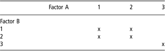
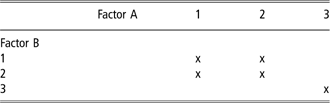
Table 1 shows an example of factor disconnectedness, where two factors, each taking three possible levels, are being investigated. In this example, factors A and B are disconnected because one cannot join all bordering pairs of cells with both horizontal and vertical links. Consequently, even in a model without any interaction terms, the effect of the third level of A cannot be estimated separately from the effect of the third level of B. This would be diagnosed differently depending on the software used with different combination of error messages in the log, zero degrees of freedom for some effects in the ANOVA table, or a missing value for the statistic used for testing.

Table 1

Example of factor disconnectedness

In general, the variance between studies is large compared to the variance within studies, hence underlying the importance of including the study effect into the meta-analytical model. The study effect represents the sum of the effects of many factors that differ between studies, but factors that are not in the model because they either were not measured, or have been excluded from the model, or for which the functional form in the model is inadequately representing the true but unknown functional form (e.g. the model assumes a linear relationship between the dependent and one independent continuous variable whereas the true relationship is nonlinear). In the absence of interactions between design variables (e.g. studies) and the covariates (e.g. all model variables of interest), parameter estimates for the covariates are unbiased, but the study effect can add a large uncertainty to future predictions (St-Pierre, Reference St-Pierre2001). The presence of significant interactions between studies and at least one covariate is more problematic since this indicates that the effect of the covariate is dependent on the study, implying that the effect of a factor is dependent on the levels of unidentified factors.

Steps in the meta-analytic process

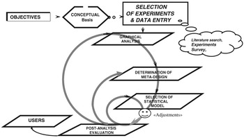
There are several inherent steps to meta-analyses, the important ones are summarized in Figure 1. An important aspect of this type of analyses is the iteration process, which is under the control of the analyst. This circular pattern where prior steps are re-visited and refined is an important aspect of meta-analyses and contributes much to their heuristic characteristic.

Figure 1

Schematic representation of the meta-analytic process.

Objectives of the study

Establishing a clear set of study objectives is a critical step that guides most ulterior decisions such as the database structure, data filtering, weighing of observations and choice of the statistical model. Objectives can cover a wide range of targets, ranging from preliminary analyses to identify potential factors affecting a system, thus serving an important role to the formulation of research hypotheses in future experiments, to the quantification of the effect of a nutritional factor such as a specific feed additive.

Data entry

Results from prior research found in the literature must be entered in a database. The structure and coding of the database must include numerous variables identifying the experimental objectives of all experiments selected. Hence, numerous columns are potentially added to code each objective found in all the sources of experimental data. This coding is necessary so as to avoid the improper aggregation of results across studies with very different objectives. During this coding phase, the analyst may chose to transform a continuous variable to a discrete variable with n levels coded in a single column with levels of the discrete variable as entries, or in n columns with 0 to 1 entries to be used as dummy variables in the meta-analytic model. Different criteria can guide the selection of classes, such as equidistant classes, or classes with equal frequencies or probability of occurrence. The important point is that the sum of these descriptive columns must entirely characterize the objectives of all studies used.

Data filtering

There are at least three steps necessary to effective data filtering. First, the analyst must ensure that the study under consideration is coherent with the objectives of the meta-analysis. That is, the meta-analytic objectives dictate that some traits must be measured and reported. If, for example, the objective of meta-analysis is to quantify the relationship between dietary neutral detergent fiber (NDF) concentration and DMI, then one must ensure that both NDF concentration and DMI were measured and reported in all studies. The second step consists of a thorough and critical review of each publication under consideration, focusing on the detection of errors in the reporting of quantitative results. This underlines the importance of having a highly trained professional involved in this phase of the study. Only after publications have passed this ‘expert’ quality filter should their results be entered in the database. Verification of data entries is then another essential component to the process. In this third step, it is important to ensure that a selected publication does not appear to be an outlier with respect to the characteristics and relations under consideration.

Preliminary graphical analyses

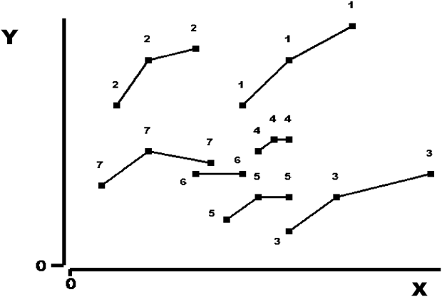
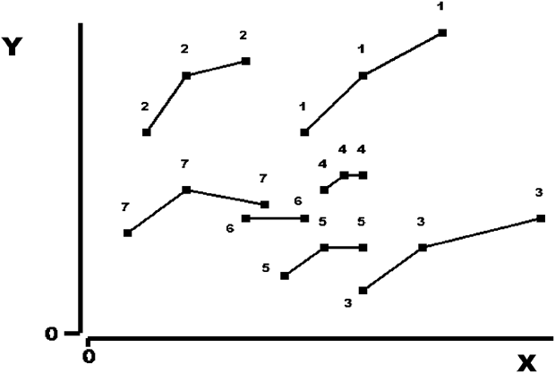
A thorough visual analysis of the data is an essential step to the meta-analytic process. During this phase, the analyst can form a global view regarding the coherence and heterogeneity of the data, as well as to the nature and relative importance of the inter- and intrastudy relationships of prospective variables taken two at a time. Systematic graphical analyses should lead to specific hypotheses and to the initial selection of alternate statistical models. Graphics can also help in identifying observations that appear unique or even outliers to the mass of all other observations. The general structure of relationships can also be identified, such as linear v. nonlinear relationships as well as the presence of interactions. As an example, Figure 2 shows a fictitious example of an intrastudy curvilinear relationship between two variables in the presence of a negative interstudy effect. In this example, the negative interstudy effect associated with the X variable indicates the presence of a latent variable that differed across studies, and that interacts with the X variable. A review of the specific characteristics of studies (3) and (2) in this example might help to identify this latent variable. This ‘visualization’ phase of the data should always be taken as a preliminary step to the statistical analysis and not as conclusive evidence. The reason is that as the multi-dimensions of the data are collapsed into two- or possibly three-dimensional graphics, the unbalance that clearly is an inherent characteristic of meta-analytic data can lead to false visual relationships. This is because X–Y graphics do not correct the observations for the effects of all other variables that can affect Y.

Figure 2

Example of a curvilinear intrastudy effect in the presence of a linear negative interstudy effect.

Graphical analyses should also be done with regard to the joint coverage of predictor variables, identifying their possible ranges, plausible ranges and joint distributions, all being closely related to the inference range. Similar X–Y graphics should be drawn to explore the relationships between predictor variables taken two at a time. In such graphics, the presence of any linear trends indicates correlations between predictor variables. Strong positive or negative correlations of predictor variables have two undesirable effects. First, they may induce near collinearity, implying that the effect of one predictor cannot be uniquely identified (i.e. is nearly confounded with the effect of another predictor). In such instances, the statistical model can include only one of the two predictors at a time. Second, the range of a predictor X ₁ given a level of a second predictor X ₂ is considerably less than the unconditional range of predictor X ₁. In these instances, although the range of a predictor appears considerable in a univariate setting, its effective range is actually very much reduced in the multivariate space.

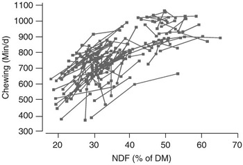
Figure 3 illustrates some of these concepts using an actual set of data on chewing activity in cattle and the NDF content of the diet. Visually, one concludes that both the intra- and interstudy relationships between chewing activity and diet NDF are nonlinear. This observation can be formally tested using the statistical methods to be outlined later. In this example, the possible NDF range is 0% to 100%, whereas its plausible range is more likely between 35% and 60%. Interestingly, the figure illustrates that experimental measurements were frequently in the 20% to 40% and 45% to 55% ranges, leaving a hole with very few observations in the 40% to 45% range.

Figure 3

Effect of dietary neutral detergent fiber (NDF) content on chewing activity in cattle. Data are from published experiments where the NDF content of the diet was the experimental treatment.

Study of the experimental meta-design

The meta-design is determined by the structure of the experiments for each of the predictor variables. To characterize the meta-design, numerous steps must take place before and after the statistical analyses. The specific steps depend on the number of predictor variables in the model.

One predictor variable

• • The experimental design used in each of the studies forming the database must be identified and coded, and their relative frequencies calculated. This information can be valuable during the interpretation of the results.

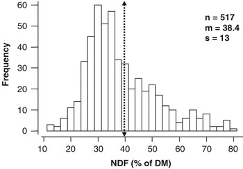
• • Frequency plots (histograms) of the predictor variable can identify areas of focus of prior research. For example, Figure 4 shows the frequency distributions of NDF for the 517 treatment groups for the meta-analytic dataset used to draw Figure 3. Figure 4 indicates a substantial research effort towards diets containing 30% to 35% NDF, an area of dietary NDF density that borders the lower limit of recommended dietary NDF for lactating dairy cows. Because of the high frequency of observations in the 30% to 35% NDF range, the a priori expectation is that the effect of dietary NDF will be estimated most precisely in this range.

  Figure 4

  Frequency plot of neutral detergent fiber (NDF) content of diets across experimental treatments.

  

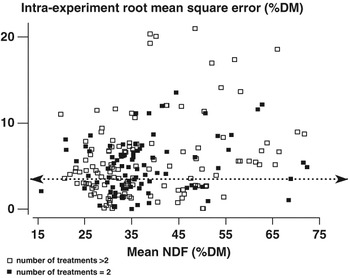
• • One should also consider the intra- and interstudy variances for the predictor variable. Small intrastudy variances reduce the ability of assessing the structural form of the intrastudy relationship between the predictor and the dependent variable. Large intrastudy variances, but with only two levels of the predictor variable, can hide any potential curvilinear relationships. Figure 5 shows the intrastudy root mean square error (S) of NDF as a function of the mean dietary NDF for experiments with two treatments, and for those with more than two treatments. The analyst can determine a minimum threshold of S to exclude experiments with little intrastudy variation in the predictor variable. In instances where the study effect is considered random, this is not necessary. In such instances, the inclusion of studies with little variation in the predictor variable does little in determining the relationship between the predictor and the dependent variable, but adds observations and degrees of freedom to estimate the variance component associated with the study effect. When looking at a possible curvilinear intrastudy relationship, it is intuitive to retain only those experiments with three or more levels of the predictor variables in the dataset. However, in Figure 5, this eliminates 40% of all the observation in the study. In instances where the curvilinear relationship is only apparent interstudy, one may chose to retain only experiments with three or more treatments, or work on the intrastudy deviation between the control and treatment groups, as suggested by Rico-Gomez and Faverdin (Reference Rico-Gomez and Faverdin2001).

  Figure 5

  Intrastudy root mean square error of dietary neutral detergent fiber (NDF) and mean NDF of experiments designed to study the effects of NDF in cattle.

  

• • Another important aspect at this stage of the analysis is to determine the significance of the study effect on the predictor variables. As explained previously, one must be very careful regarding the statistical model used to investigate the intrastudy effect when there is not a good agreement between the intra- and interstudy effects. In these instances, the relationship between the predictor variable and the dependent variable depends on the study, which itself represents the sums of a great many factors such as measurement errors, systematic differences in the methods of measurements of the dependent variable across studies, and, more importantly, latent variables (hidden) not balanced across experiments. In those instances, the analyst must exert great caution in the interpretation of the results, especially regarding the applicability of these results.

• • At this stage, even before statistical models are to be fitted and effects tested, it is generally useful to calculate the leverage of each observation (Tomassone et al., Reference Tomassone, Lesquoy and Millier1983). Traditionally, in statistics, leverage values are calculated after the model is fitted to the data, but nothing prohibits the calculation of leverage values at an earlier stage because their calculations depend only on the design of the predictor variable in the model. For example, in the case of the simple linear regression with n observations, the leverage point for the ith observation is calculated as

(1)

where h_i is the leverage value, X_i is the value of the ith predictor variable and X_m is the mean of all X_i.

Equation (1) clearly indicates that the leverage of an observation, i.e. its weight in the determination of the slope, grows with its distance from the mean of the predictor variable. The extension of the leverage point calculations to more than one predictor variables is straightforward (St-Pierre and Glamocic, Reference St-Pierre and Glamocic2000).

• • In a final step, the analyst must graphically investigate the functional form of the relationship between the dependent variable and the predictor variable.

Two or more predictor variables: In the case of two or more predictor variables, the analyst must examine graphically and then statistically the inter- and intrastudy relationships between the predictor variables. Leverage values should be examined. With fixed models (all effects in the models are fixed with the exception of the error term), variance inflation factors (VIFs) should be calculated for each predictor variable (St-Pierre and Glamocic, Reference St-Pierre and Glamocic2000). An equivalent statistic has not been proposed for mixed models (e.g. when the study effect is random), but asymptotic theory would support the calculation of the VIFs for the fixed effect factors in cases where the total number of observations is large. The objective in this phase is to assess the degree of inter-dependence between the predictor variables. Because predictor variables in meta-analyses are never structured prior to their determination, they are always non-orthogonal and, hence, show variable degrees of inter-dependency. Collinearity determinations (VIFs) assess one’s ability to separate the effects of inter-dependent factors based on a given set of data. Collinearity is not model driven, but completely data driven.

Weighing based on classical statistical theory

Under a general linear model where observations have heterogeneous but known variances, maximum likelihood parameters estimates are obtained by weighing each observation by the inverse of its variance. In the context of a meta-analysis where observations are least-squares (or population marginal) means, observations should be weighed by the inverse of the squares of their standard errors, which are the standard errors of each mean (s.e.). Unfortunately, when such weights are used, the resulting measures of model errors (i.e. standard error, standard error of predictions, etc.) are no longer expressed in the original scale of the data. To maintain the expressions of dispersion in the original scale of the measurements, St-Pierre (Reference St-Pierre2001) suggested dividing each weight by the mean of all weights, and to use the resulting values as weighing factors in the analysis. Under this procedure, the average weight used is algebraically equal to 1.0, thus resulting in expressions of dispersion that are in the same scale as the original data. The application of this technique is software dependent. In the Statistical Analysis System (SAS), for example, weights are automatically rescaled so that their sums must be equal to 1.

Weighing based on other criteria

Other weighing criteria have been suggested for the weighing of observations, such as the power of an experiment to detect an effect of a size defined a priori, the duration of an experiment, etc. The weighing scheme can actually be based on an expert assessment, partially subjective, of the overall quality (precision) of the data. The opinion of more than one expert may be useful in this context. From a Bayesian statistical paradigm, the use of subjective information for decision-making is perfectly coherent and acceptable, as subjective probabilities are often used to establish prior distributions in Bayesian decision theory (De Groot, Reference De Groot1970). Traditional scientific objectiveness, however, may restrict the use of this weighing scheme in scientific publications.

Predictably, the importance of weighing observations decreases with the number of observations used in the analysis, especially if the observations that would receive a small weight have relatively small leverage values. For example, we conducted a meta-analysis to quantify the effect of concentrate intake on milk production and intake by dairy cows (Sauvant et al., personal communication). The data, consisting of 208 treatment means from 85 experiments that had as a primary objective to study the effect of concentrate intake, were analyzed with and without a weighing scheme based on the reciprocals of the s.e. The resulting weights ranged between 0.25 and 12.5. The functional structure of the response was a quadratic function with fixed study effect. In the example, the dependent variable was DMI (kg/day). The independent variable (predictor) was concentrate DMI (CI, kg/day). For DMI, the estimated function using unweighed observations was

(2)

The same function estimated using weighed observations was:

(3)

Clearly, the regression coefficients of (2) and (3) are very close to each other and do not lead to much difference in the predicted response to CI.

Whether the analyst should weight the observations based on the s.e. for each individual treatments or the pooled s.e. from the studies is open to debate. There are many reasons why the s.e. of each treatment within a study can be different. First, the original observations themselves could have been homoscedastic (homogeneous variance) but the least-squares means would have different s.e. due to unequal frequencies (e.g. missing data). In such a case, it is clear that the weight should be based on the s.e. of each treatment. Second, the treatments may have induced heteroscedasticity, meaning that the original observations did not have equal variances across sub-classes. In such instances, the original authors should have conducted a test to assess the usual homoscedasticity assumption in linear models. The problem is that a lack of significance (i.e. P > 0.05) when testing the homogeneity assumption does not prove homoscedasticity, but only that the null hypothesis (homogeneous variance) cannot be rejected at a P < 0.05. In a meta-analytic setting, the analyst may deem the means with larger apparent variance to be less credible and reduce the weight of these observations in the analysis. Unfortunately, most publications lack the information necessary for this option.

Among the more subjective criteria available for weighing is the quality of the experimental design used in the original study with regard to the meta-analytic objective. Experimental designs have various trade-offs due to their underlying assumptions. For example, the Latin square is often used in instances where animal units are relatively expensive, such as in metabolic studies. The double orthogonal blocking used to construct Latin square designs can remove a lot of variation from the residual error. Thus very few animals can be used compared to a completely randomized design for an equal power of detecting treatment effect. The downside, however, is that the periods are generally relatively short to reduce the likelihood of a period by treatment interaction (animals in different physiological status across time periods), thus reducing the magnitude of the treatment effects on certain traits, such as production and intake, for example. In those instances, the analyst should legitimately weigh down observations from experiments whose designs limited the expression of the treatment effects.

Statistical models

The independent variable can be either discrete or continuous. With binary data (healthy/sick, for example), generalized linear models (GLM) based on the logit or probit link functions are generally recommended (Agresti, Reference Agresti2002). Because of advances in computational power, the GLM has been extended to include random effects in what is called the generalized linear mixed model (GLMM). In its version 9, the SAS system includes a beta release of the GLIMMX procedure to fit these complicated models. In nutrition, however, the large majority of the dependent variables subjected to meta-analyses are continuous, and their analyses are treated at length in the remainder of this paper.

St-Pierre (Reference St-Pierre2001) made a compelling argument to include the study effect in all meta-analytic models. Because of the severe imbalance in most databases used for meta-analyses, the exclusion of the study effect in the model leads to biased parameter estimates of the effects of other factors under investigation, and severe biases in variance estimates. In general, the study effect should be considered random because it represents, in essence, the sum of the effects of a great many factors, all with relatively small effects on the dependent variable. Statistical theory indicates that these effects would be close to Gaussian (normal), thus much better estimated if treated as random effects. Practical recommendations regarding the selection of the type of effect for the studies are presented in Table 2. In short, the choice depends on the size of the conceptual population, and the sample size (the number of studies in the meta-analysis).

Table 2

Guidelines to establish whether an effect should be considered fixed or random in a meta-analytic model*

*Adapted from Milliken (1999) for mixed models.

^†T represents the number of studies in the population (conceptual), and t is the number of studies in the meta-analysis.

The ultimate (and correct) meta-analysis would be one where all the primary (raw) data used to perform the analyses in each of the selected publications were available to the analyst. In such an instance, a large segmented model that includes all the design effects of the original studies (e.g. the columns and rows effects in Latin squares) plus the effects to be investigated by the meta-analysis could be fitted by least-squares or maximum likelihood methods. Although computationally complex, such huge meta-analytic models should be no more difficult to solve than the large models used by geneticists to estimate the breeding values of animals using very large national databases of production records. Raw data availability should not be an issue in instances where meta-analyses are conducted with the purpose of summarizing research at a given research center. This, however, is very infrequent, and meta-analyses are almost always conducted using observations that are themselves summaries of prior experiments (i.e. treatment means). It seems evident that a meta-analysis conducted on summary statistics should lead to the same results as a meta-analysis conducted on the raw data, which itself would have to include a study effect because the design effects are necessarily nested within studies (e.g. cow 1 in the Latin square of study 1 is different from the cow 1 of study 2), which itself would likely be considered random. Thus, analytical consistency dictates the inclusion of the study effect in the model, generally as a random effect. The study effect will be considered random in the remainder of this paper, with the understanding that under certain conditions explained previously it should be considered a fixed effect factor.

Besides the study effect, meta-analytic models include one or more predictor variables that are either discrete or continuous. For clarity, we will initially treat the case of each variable type separately, understanding that a model can easily include a mixture of variables of both types, as we describe later.

Model with discrete predictor variable(s)

A linear mixed model easily models this situation as follows:

(4)

where Y_ijk = the dependent variable, μ = overall mean, S_i = the random effect of the ith study, assumed∼_iidN (0, σ ²_S), τ_j = the fixed effect of the jth level of factor τ, Sτ_ij = the random interaction between the ith study and the jth level of factor τ, assumed∼_iidN (0, σ ²_Sτ), and e_ijk = the residual errors, assumed∼_iidN (0, σ ²_e). e_ijk, Sτ_ij and S_i are assumed to be independent random variables.

For simplicity reasons, model (4) is written without weighing the observations. The weights would appear as multiplicative factors of the diagonal elements of the error variance-covariance matrix (Draper and Smith, Reference Draper and Smith1998). Model (4) corresponds to an incomplete, unbalanced randomized block design with interactions in classic experimental research. The following SAS statements can be used to solve this model:

(5)

Standard tests of significance on the effect of τ are easily conducted and least-squares means can be separated using an appropriate mean separation procedure. Although it may be tempting to remove the study effect from the model in instances where it is not significant (also called pooling of effects), this practice can lead to biased probability estimations (i.e. final tests on fixed effects are conditional on tests for random effects) and is not recommended. This is because not being able to reject the null hypothesis of no study effect (i.e. variance due to study is not significantly different from zero) is a very different proposition than proving that the effect of the study is negligible. At the very least, the probability threshold for significance of study should be much larger than the traditional P = 0.05 (say P < 0.25). Ideally, the analyst should state before the analysis is performed what size of estimated variance due to study should be considered negligible, such as .

Model with continuous predictor variable(s)

A linear mixed model also easily models this situation.

(6)

where Y_ij = the dependent variable, B ₀ = overall (interstudy) intercept (a fixed effect equivalent to μ in (4)), S_i = the random effect of the ith study, assumed∼_iidN (0, ), B ₁ = the overall regression coefficient of Y on X (a fixed effect), X_ij = the value of the continuous predictor variable, b_i = the random effect of study on the regression coefficient of Y on X, assumed∼_iidN (0, ), and e_ij = the residual errors, assumed∼_iidN (0, ). Also, e_ij, b_i and S_i are assumed to be independent random variables.

The following SAS statements can be used to solve this model:

(7)

Using a simple Monte Carlo simulation, St-Pierre (Reference St-Pierre2001) demonstrated the application of this model to a synthetic dataset, showing the power of this approach, and the interpretation of the estimated parameters.

Model with both discrete and continuous predictor variable(s)

Statistically, this model is a simple combination of (4) and (6) as follows:

(8)

where B_j = the effect of the jth level of the discrete factor τ on the regression coefficient (a fixed effect).

The following SAS statements would be used to solve this model:

(9)

In theory, (8) is solvable, but the large number of variance components and interaction terms that must be estimated in combination with the imbalance in the data makes it often numerically intractable. In such instances, at least one of the two random interactions must be removed from the model.

In (4), (6) and (8), the analyst secretly wishes for the interactions between study and the predictor variables to be highly non-significant. Recall that the study effect represents an aggregation of the effects of many uncontrollable and unknown factors that differed between studies. A significant study by factor τ interaction (Sτ_ij) in (4) implies that the effect of τ is dependent on the study, hence of factors unaccounted for. Similarly, a significant interaction of study by X in (6) (b_i X_ij) indicates that the slope of the linear relationship of Y on X is dependent on the study, hence of unidentified factors. In such a situation, the analysis produces a model that can explain very well the observations, but predictions of future outcomes are generally not precise because the actual realization of a future study effect is unknown. The maximum likelihood predictor of a future observation is produced by setting the study and the interaction of study with the fixed effect factors to their mean effect values of zero (McCulloch and Searle, Reference McCulloch and Searle2001), but the standard error of this prediction is very much amplified by the uncertainty regarding the realized effect of the future study.

When the study effect and its interaction with fixed effect is correctly viewed as an aggregation of many factors not included in the model, but that differed across studies, the desirability of including as many fixed factors in the model as can be uniquely identified from the data becomes obvious. In essence, the fixed effects should ultimately make the study effect and its interactions with fixed effects predictors small and negligible. In such instances, the resulting model should have wide forecasting applicability. Imagine, for example, that much of the study effect on body weight gain of animal is in fact due to the large difference in the initial body weight across studies. In such instances, the inclusion of initial body weight as a covariate would remove much of the study effect, and the diet effects (as continuous or discrete variables) would be estimated without biases, with a wide range of applicability (i.e. a future prediction would require a measurement of initial body weight as well as measurements of the other predictor variables).

Whether one chooses (4) or (6) as a meta-model is somewhat arbitrary when the predictor variable has an inherent scale (i.e. is a measured number). The assumptions regarding the relationship between Y and the predictor variable are, however, very different between the two models. In (4), the model does not assume any functional form for the relationship. In (6), the model explicitly assumes a linear relationship between the dependent and the predictor variables. Different methods can be used to determine whether the relationship should have a linear or nonlinear structure.

• • The first method consists in classifying observations into five sub-classes based on the quintiles for the predictor variable, and performing the analysis according to (4) with five discrete levels of the predictor variable. Although the selection of five sub-classes is somewhat arbitrary, there are substantive references in the statistical literature indicating that this number of levels generally works well (Cochran, Reference Cochran1968; Rubin, Reference Rubin1997). A visual inspection of the five least-squares means or the partitioning of the four degrees of freedom associated with the five levels of the discrete variable into singular orthogonal polynomial contrasts can rapidly identify an adequate functional form to use for modeling the Y–X relationship.

• • The second method can be directly applied to the data, or can be a second step that follows the identification of an adequate degree for a polynomial function. Model (6) is augmented with the square (and possibly higher order terms) of the predictor variable. In the MIXED procedure of SAS, this can be done simply by adding an X*X term to the model statement. It is important to understand that in the context of a linear (mixed or not) model, the matrix representation of the model and the solution procedure used are no different when X and X ² are in the model compared to a situation where two different continuous variables (say X and Z) are included in the model. The problem, however, is that X and X ² are implicitly not independent; after all, there is an algebraic function relating the two. This dependence can result in a large correlation between the two variables, thus leading to possible problems of collinearity.

• • A third method can be used in more complex situations where the degree of the polynomial exceeds two, or the form of the relationship is sigmoid, for example. The relationship can be modeled as successive linear segments, an approach conceptually close to the first method explained previously. Martin and Sauvant (Reference Martin and Sauvant2002) used this method to study the variation in the shape of the lactation curves of cows subjected to various concentrate supplementation strategies, using the model of Grosman and Koops (Reference Grosman and Koops1988) as its fundamental basis. Using this approach, lactation curves were summarized by a vector of nine parameter estimates, whose estimates could be compared across supplementation strategies.

In (8), the interest may be in the effect of the discrete variable τ after adjusting for the effect of a continuous variable X as in a traditional covariate analysis, or the interest may be inverse, i.e. the interest is in the effect of the continuous variable after adjusting for the effect of the discrete variable. The meta-analyses of Firkins et al. (Reference Firkins, Eastridge, St-Pierre and Noftsger2001) provide examples of both situations. In one instance, the effect of grain processing (a discrete variable) on milk fat content was being investigated while correcting for the effect of DMI (a continuous variable). In this instance, the interest was in determining the effect of the discrete variable. In another instance, the effects of various dietary factors such as dietary NDF, DMI and the proportion of forage in the diet (all continuous variables) on starch and NDF digestibility, and microbial N synthesis were investigated, while correcting for the effect of the grain processing. In this case, the interest was much more towards the effects of the continuous variables exempt from possible biases due to different grain processing across experiments.

Accounting for interfering factors

Differences in experimental conditions between studies can affect the treatment response. The nature of these conditions can be represented by quantitative or qualitative variables. In the first instance, the variable and possibly its interaction with other factors can be added to the model if there are sufficient degrees of freedom. The magnitude of treatment response is sometimes dependent on the observed value in the control group. For example, the milk fat response in lactating cows to dietary buffer supplementation as a function of the milk fat of the control group (Meschy et al., Reference Meschy, Bravo and Sauvant2004). The response was small or non-existent when the milk fat of control cows was near 40 g/l, but increased markedly when the control cows had low milk fat, possibly reflecting a higher likelihood of sub-clinical rumen acidosis in these instances.

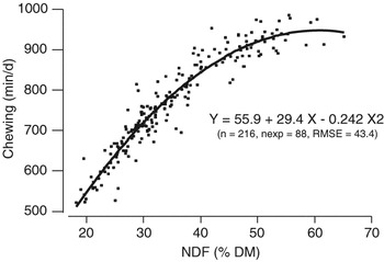
When the intrastudy response depends on the levels of the predictor variable, it is often because of the existence of a nonlinear interstudy relationship. Applying model (6) with the addition of a square term for the X_ij to the data shown in Figure 3 results in a relatively good quantification of the relationship between chewing time and dietary NDF, as shown in Figure 6. In this type of plot, it is important to adjust the observations for the study effect, or the regression may appear to poorly fit the data because of the many hidden dimensions represented by the studies (St-Pierre, Reference St-Pierre2001).

Figure 6

Effect of dietary neutral detergent fiber (NDF) content on chewing activity in cattle. Data are from published experiments where the NDF content of the diet was the experimental treatment. Observations were adjusted for the study effect before being plotted, as suggested by St-Pierre (Reference St-Pierre2001). n = number of treatments; nexp = number of experiments.

In instances where the interacting factor is discrete, the examination of the sub-classes least-squares means can clarify the nature of the interaction. For example, the effect of a dietary treatment may be dependent on the physiological status of the animals used in the study. This physiological status can be coded using multiple dummy variables, as explained previously.

Structure of residual variation

In (4), (6) and (8), the residuals (errors) are assumed independent, and identically distributed from a normal population with a mean of zero and a variance . The normality assumption can be tested using a standard χ ² test, or a Shapiro-Wilks test, both available in the UNIVARIATE procedure of the SAS system. The residuals can also be expressed as Studentized residuals, with absolute values exceeding 3 being suspected as outliers (Tomassone et al., Reference Tomassone, Lesquoy and Millier1983). In meta-analysis, the removal of a suspected outlier observation should be done only with extreme caution. This is because the observations in a meta-analysis are the calculated outcomes (least-squares means) of models and experiments that should themselves be nearly free of the influence of outliers. Thus, meta-analytic outliers can be much more likely indicative of a faulty model than of a defective observation. In addition, the removal of one treatment mean as an observation in a meta-analysis might be removing all the variation in the predictor variable for the experiment in question, thus making the value of the experiment in a meta-analytic setting nearly worthless. In addition, the analyst should examine for possible intra- and interstudy relationships between the residuals and the predictor variables.

Structure of study variation

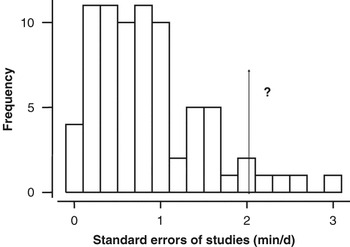
When a model of the type described in (4) is being fitted, it is possible to examine each study on the basis of its own residuals. For example, Figure 7 shows the distribution of the residual standard errors for the different studies used in the meta-analysis of chewing time in cattle (Figures 3 and 6). Predictably, the distribution is asymmetrical and follows the law of Raleigh for the standard errors, while variances have a χ ² distribution. Studies with unusual standard errors, say those with a χ ² probability exceeding 0.999, could be candidates for exclusion from the analysis. Alternatively, one could consider using the inverse of the estimated standard errors as weights to be attached to the observation before re-iterating the meta-analysis.

Figure 7

Frequency distribution of the residual standard errors of the studies used in the meta-analysis of chewing activity in cattle.

Other calculations such as leverage values, Cook’s distances and other statistics can be used to determine the influence of each observation on the parameter estimates (Tomassone et al., Reference Tomassone, Lesquoy and Millier1983).