3.1. Stability threshold

Unlike the flat-plate scenario, the liquid film flow on a conical surface is non-parallel even when the disturbances are absent. This dependence of the base flow on the streamwise coordinate usually demands special consideration in linear stability analysis (Govindarajan & Narasimha Reference Govindarajan and Narasimha1995, Reference Govindarajan and Narasimha1997; Bertolotti Reference Bertolotti1997; Herbert Reference Herbert1997). For the presently studied conical liquid film flow, Zollars & Krantz (Reference Zollars and Krantz1980) derived an asymptotic base-flow solution from the Navier–Stokes equations, and performed a spatial linear stability analysis with respect to axisymmetric disturbances. However, their results only contained the effect of lateral curvature of the gas–liquid interface. The streamwise curvature was not included due to its smaller order of magnitude (see (2.20)) in their first-order model.

In this section, we revisit the spatial linear stability problem with a similar approach to that of Zollars & Krantz (Reference Zollars and Krantz1980), extending it to second order and paying special attention to the influence of the streamwise curvature. Instead of employing the streamfunction as is done in Zollars & Krantz (Reference Zollars and Krantz1980), however, the present analysis is based on a Benney-type equation derived below. For liquid film flow on a flat plate, the cutoff wavenumber obtained from the Benney equation (Benney Reference Benney1966) coincides with that from the long-wave expansion of the Orr–Sommerfeld equation (Kalliadasis et al. Reference Kalliadasis, Ruyer-Quil, Scheid and Velarde2012, § 5.1.5).

We expand the variables $u (r, \alpha , t)$ , $v (r, \alpha , t)$ and $p (r, \alpha , t)$ in powers of $\varepsilon$

(3.1a) \begin{align} u & = u^{(0)} + \varepsilon u^{(1)} + \varepsilon ^2 u^{(2)} + O\bigl(\varepsilon ^3\bigr), \end{align}

(3.1b) \begin{align} v & = v^{(0)} + \varepsilon v^{(1)} + O\bigl(\varepsilon ^2\bigr), \end{align}

(3.1c) \begin{align} p & = p^{(0)} + \varepsilon p^{(1)} + O\bigl(\varepsilon ^2\bigr). \end{align}

Equations (3.1) are substituted into (2.13)–(2.15). The terms with superscripts $(0)$ , $(1)$ and $(2)$ can be solved sequentially. Expressions of these terms are given in (B1)–(B6) in Appendix B for reference. Specifically,

(3.2) \begin{equation} u^{(0)} = - r^2 \psi ^2 \left (\frac {\alpha }{\psi } - \frac {1}{2} \frac {\alpha ^2}{\psi ^2}\right ) \cos \beta . \end{equation}

In dimensional form, $\tilde {u}^{(0)} = - g \tilde {h}^2 \cos \tilde {\beta }/(2\nu )$ at the free surface $\tilde \alpha =\tilde \psi$ . This justifies the choice of the velocity scale $U=gH^2/\nu$ in § 2.

The solution (3.1a ) is substituted into (2.21) through the definition of $\tilde q$ in (2.9), i.e.

(3.3) \begin{equation} \frac {\partial h}{\partial t} = \frac {1}{r \sin (\beta - \varepsilon h / r)} \frac {\partial }{\partial r} \int _{0}^{\psi } r^2 \left (u^{(0)} + \varepsilon u^{(1)} + \varepsilon ^2 u^{(2)}\right ) \sin (\beta + \varepsilon \alpha ) \,\text{d}\alpha . \end{equation}

The integral and derivative operations on the right-hand side are straightforward after performing Taylor expansion for the sinusoidal functions. The final result, being a little lengthy, is given by (B7)–(B10) in Appendix B (some of the symbolic manipulations in this paper were carried out using the Python library SymPy 1.13 (Meurer et al. Reference Meurer2017)). Equation (3.3) is the second-order Benney-type equation for liquid film flow along a conical surface.

Next, we seek the steady-state film thickness $\bar h$ at fixed flow rate $q=q_s$ by writing

(3.4) \begin{equation} \bar h = \bar h^{(0)} + \varepsilon \bar h^{(1)} + \varepsilon ^2 \bar h^{(2)} + O \bigl( \varepsilon ^3 \bigr). \end{equation}

After replacing $h$ with $\bar h$ and setting $\partial \bar h/\partial t=0$ in (3.3), $\bar h^{(0)}$ , $\bar h^{(1)}$ and $\bar h^{(2)}$ are solved successively as

(3.5) \begin{align} \bar h^{(0)} &= K (q_s / r)^{1/3}, \end{align}

(3.6) \begin{align} \bar h^{(1)} &= - \frac {4 K^{2} {\textit{Re}} q_s^{5/3}}{35 r^{8/3} \sin \beta } + \frac {K^{2} q_s^{2/3} \sin \beta }{9 r^{5/3} \cos \beta } + \frac {K^{2} q_s^{2/3} \cos \beta }{3 r^{5/3} \sin \beta } - \left (\frac {\varepsilon }{{\textit{Bo}}}\right ) \frac {K q_s^{1/3}}{3 r^{7/3} \sin \beta }, \\[9pt] \nonumber \end{align}

and

(3.7) \begin{align} \bar h^{(2)} &= \frac {19648 {\textit{Re}}^{2} q_s^{3}}{121275 r^{5} \sin ^{3}\beta \cos \beta } + \frac {32 {\textit{Re}} q_s^{2}}{105 r^{4} \sin \beta \cos ^{2}\!\beta } + \frac {83 {\textit{Re}} q_s^{2}}{140 r^{4} \sin ^{3}\beta } - \frac {7 q_s \sin \beta }{27 r^{3} \cos ^{3}\!\beta }\nonumber \\&\quad - \frac {67 q_s}{24 r^{3} \sin \beta \cos \beta } - \frac {27 q_s \cos \beta }{40 r^{3} \sin ^{3}\beta } - \frac {7 q_s}{40 r^{3} \sin ^{3}{\beta } \cos {\beta }} \nonumber \\&\quad + \!\left (\frac {\varepsilon }{{\textit{Bo}}} \!\right ) \!\left [\! - \frac {4 K^{2} {\textit{Re}} q_s^{5/3}}{105 r^{14/3} \sin ^{2}\!\beta } - \frac {40 K^{2} q_s^{2/3}}{81 r^{11/3} \cos \beta } - \frac {K^{2} q_s^{2/3} \cos \beta }{r^{11/3} \sin ^{2}\!\beta } + \! \left (\frac {\varepsilon }{{\textit{Bo}}}\right ) \! \frac {2 K q_s^{1/3}}{9 r^{13/3} \sin ^{2}\!\beta }\!\right ]\!, \end{align}

where the constant $K = - \sqrt [3]{3 / (\sin \beta \cos \beta )}$ is positive if $\beta \gt \pi /2$ . This base-flow solution is used in the subsequent linear stability analysis. Zollars & Krantz (Reference Zollars and Krantz1976) also derived a first-order asymptotic expression for the steady-state film thickness by applying a perturbation expansion to the streamfunction. Truncating our result at the same order, i.e. $\bar h^{(0)} + \varepsilon \bar h^{(1)}$ , reproduces their formula once their scaling is adopted. These expressions for $\bar h$ are expected to be valid except in the vicinity of the cone axis (see § 7.1 for more discussion).

Before proceeding, it might be interesting to examine the shapes of the undisturbed film flow predicted by (3.4). However, the dependence of the dimensionless quantities on the unspecified length scales $H$ and $L$ causes inconvenience in displaying results and describing liquid properties/working conditions. It is noteworthy that $H$ and $L$ (thus $\varepsilon$ ) are introduced to simplify the governing equations by distinguishing the orders of different terms explicitly. Once the final results, e.g. (3.4), are obtained, it would be useful to re-nondimensionalise the variables with a more specific length scale such as the film thickness at the inlet, $\tilde h_{\textit{in}}$ , or the combination $(\nu ^2/g)^{1/3}$ . Actually, on substitution of $L=H=(\nu ^2/g)^{1/3}$ , one finds

(3.8) \begin{equation} {\textit{Re}} = \frac {g H^3}{\nu ^2} = 1, \quad {\textit{Bo}} = \frac {\rho g H^2}{\sigma } = \frac {\rho g^{1/3} \nu ^{4/3}}{\sigma } \equiv \frac {1}{{Ka}_\perp }, \quad q = \frac {\tilde q}{U H L} = \frac {\tilde q g^{1/3}}{\nu ^{5/3}} \equiv N_{q\perp }, \end{equation}

i.e. $Re$ is always 1; the original Bond number converts to a form whose inverse is usually designated to the Kapitza number, ${Ka}_\perp$ ; and the non-dimensionalised flow rate $q$ becomes $N_{q\perp }$ . The subscript $\perp$ indicates the dimensionless groups are ‘vertical’ versions that are irrelevant to the angle $\tilde \beta$ .

Figure 2 shows $\tilde {\bar h}$ as a function of $\tilde r$ predicted by (3.4) at four different $\tilde \beta$ . The other parameters are fixed as ${Ka}_\perp = 242$ and $N_{q\perp } = 1703$ . For an aqueous glycerol solution with $\nu = 5.77 \times 10^{-6}\, \mathrm{m^2}\, \mathrm{s}^{-1}$ (case C in Denner et al. (Reference Denner, Charogiannis, Pradas, Markides, van Wachem and Kalliadasis2018)), this $N_{q\perp }$ corresponds to a dimensional volumetric flow rate of $\tilde Q = 2 \pi \tilde q = 9.28 \times 10^{-6}\,\mathrm{m}^3\,\mathrm{s}^{-1}$ . Interestingly, all four curves in figure 2 are nearly parallel to each other. With the same volumetric flow rate, the film thickness at the same radial position decreases as $\tilde \beta$ increases from $100^\circ$ to $135^\circ$ . However, further increasing $\tilde \beta$ leads to a higher elevation of the film surface. Moreover, except for the very small region close to the apex, the result with $\tilde \beta =160^\circ$ is almost indistinguishable from that with $\tilde \beta =110^\circ$ .

Figure 2.

Steady-state film thickness (3.4) versus radial distance at different $\tilde {\beta }$ . ${Ka}_\perp = 242$ , $N_{q\perp } = 1703$ .

The above observation results from the fact that the corrections $\bar h^{(1)}$ and $\bar h^{(2)}$ to $\bar h^{(0)}$ are negligible unless in regions where $r$ is small (the powers of $r$ in the denominators successively increase from $\bar h^{(0)}$ to $\bar h^{(2)}$ , indicating faster decay with $r$ for high-order corrections). As a consequence, the film shape is dominated by $\bar h^{(0)}$ (3.5), which, on substitution of $K$ , yields

(3.9) \begin{equation} \bar h^{(0)} = - \left ( \frac {3 q_s}{r \sin \beta \cos \beta } \right )^{1/3} = - \left [ \frac {6 q_s}{r \sin (2\beta )} \right ]^{1/3}. \end{equation}

Note that the dimensional form of (3.9) is exactly the same as (1.5). Obviously, (3.9) indicates that $\bar h^{(0)}(\beta )$ is symmetric about $\beta = 3\pi /4$ or $\tilde \beta = 135^\circ$ . This explains the overlap of the film surface for $\tilde \beta =110^\circ$ and $160^\circ$ in figure 2.

This non-monotonic behaviour can be interpreted as below: as $\tilde \beta$ increases from $90^\circ$ to $180^\circ$ , i.e. when the cone becomes progressively sharper, there are two competing mechanisms that can affect the film thickness at a fixed position $\tilde r$ . On the one hand, the local volumetric flow rate per unit width is calculated as $\tilde Q_{\mathrm{2D}} = \tilde Q / (2 \pi \tilde r \sin \tilde \beta )$ , which increases with $\tilde {\beta }$ . Thus, the film thickness also has a tendency to increase. On the other hand, the streamwise component of the gravitational acceleration $-g\cos \tilde \beta$ increases. The liquid in the film is therefore accelerated to gain a higher mean velocity, resulting in a thinner film at a fixed flow rate. Consequently, the actual film thickness is determined jointly by the geometric and dynamic factors, which are associated with $\sin \beta$ and $-\cos \beta$ in (3.9), respectively.

Notably, the existence of a minimal film thickness at a given flow rate might be helpful in designing heat- and mass-transfer equipment, as a thinner film has a smaller resistance for the transport process between the wall and the gas side.

In order to perform the stability analysis, we express the film thickness as the sum of the base flow and a small disturbance $\hat h \ll 1$

(3.10) \begin{equation} h = \bar h (r) + \hat h(r,t). \end{equation}

After substitution of (3.10), (3.3) can be linearised by dropping all terms containing second- and higher-order powers of $\hat h$ . The result is

(3.11) \begin{align} \frac {\partial \hat h}{\partial t} + S_0 \hat h + S_1 \frac {\partial \hat h}{\partial r} + S_2 \frac {\partial ^{2} \hat h}{\partial r^{2}} + S_3 \frac {\partial ^{3} \hat h}{\partial r^{3}} + S_4 \frac {\partial ^{4} \hat h}{\partial r^{4}} = 0. \end{align}

The coefficients $S_0$ – $S_4$ are given by (B11)–(B15) in Appendix B.

On the basis of (3.11), we conduct a spatial linear stability analysis. Assuming the disturbance is periodic in time and grows/decays in space, we set

(3.12) \begin{equation} \hat h(r, t) = R(r) e^{\mathrm j \omega t}, \end{equation}

where $\mathrm j$ is the imaginary unit, and $\omega$ , denoting the dimensionless angular frequency of the disturbance, is a real number. Substitution of (3.12) into (3.11) leads to an equation for $R(r)$ . Following Zollars & Krantz (Reference Zollars and Krantz1980), we assume $R(r)$ is expressed as

(3.13) \begin{equation} R(r) = e^{f_0(r) + \varepsilon f_1(r) + \varepsilon ^2 f_2(r) + O \bigl(\varepsilon ^3\bigr)}, \end{equation}

where the functions $f_i(r)$ ( $i=0$ , 1, 2) are complex in general and solved sequentially. Their expressions are listed in (B16)–(B21) of Appendix B. By taking the real part in the final result, $\hat h$ reads

(3.14) \begin{equation} \hat {h}(r, t) = C \frac {e^{B r}}{r^{1/3}} \cos \left (\omega t - A r \right )\!, \end{equation}

where

(3.15) \begin{align} A &= - \left [\textrm {Im} (f_0) + \varepsilon \textrm {Im} (f_1) + \varepsilon ^2 \textrm {Im} (f_2) \right ] / r, \end{align}

(3.16) \begin{align} B &= \left [\varepsilon \textrm {Re} (f_1) + \varepsilon ^2 \textrm {Re} (f_2)\right ] / r, \end{align}

and $C$ is an integral constant. In (3.15) and (3.16), $\textrm {Re} (\boldsymbol{\cdot })$ and $\textrm {Im} (\boldsymbol{\cdot })$ denote the real and imaginary parts of a complex number, respectively.

It is noteworthy that, at large radial distance $r$ , $B$ is dominated by

(3.17) \begin{equation} - \varepsilon ^2 \left (\frac {\varepsilon }{{\textit{Bo}}}\right ) \frac {K^{2} \omega ^{4} r^{7/3} \sin \beta }{270 q_s^{7/3} \cot ^{2}\beta }, \end{equation}

which is always negative. Noting (3.14), this fact indicates that for any given $\omega$ , the amplitude of the disturbance $\hat h$ decays to zero at large $r$ , i.e. the flow ultimately stabilises.

Within a certain range of moderate $r$ , however, the disturbances can be amplified locally. Zollars & Krantz (Reference Zollars and Krantz1980) classified the instability of this non-parallel flow into two types: the absolute growth refers to the scenario in which the raw disturbance amplitude increases with $r$ , i.e. $\text{d}[\exp {( {\textit{Br}}) / r^{1/3}}] / \text{d}r \gt 0$ ; whereas the relative growth means an increase of the amplitude scaled by the local mean film thickness $\bar h$ whose value is given in (3.4), i.e. $\text{d}[\exp {( {\textit{Br}}) / (\bar h r^{1/3}})] / \text{d}r \gt 0$ . Correspondingly, two modified spatial amplification factors can be defined as

(3.18) \begin{equation} G_a \equiv \frac {1}{\exp {( {\textit{Br}}) / r^{1/3}}} \frac {\text{d}\left[\exp {( {\textit{Br}}) / r^{1/3}}\right]}{\text{d}r} = r \frac {{\rm d} B}{\text{d}r} + B - \frac {1}{3 r} \end{equation}

for absolute growth and

(3.19) \begin{equation} G_r \equiv \frac {1}{\exp {( {\textit{Br}}) / \bigl(\bar h r^{1/3}}\bigr)} \frac {\text{d}\left[\exp {( {\textit{Br}}) / \bigl(\bar h r^{1/3}}\bigr)\right]}{\text{d}r} = r \frac {{\rm d} B}{\text{d}r} + B - \frac {1}{\bar h} \frac {\partial \bar h}{\partial r} - \frac {1}{3 r} \end{equation}

for relative growth (the definition of $G_r$ differs from that in Zollars & Krantz (Reference Zollars and Krantz1980)). The difference between the two expressions is the term $-(\partial \bar h/\partial r ) / \bar h$ , which is positive since $\bar h$ is negatively correlated with $r$ , see (3.5). Therefore, this term has a destabilising effect, and it is possible that, at the same $r$ , a flow is stable in the sense of absolute growth ( $G_a\lt 0$ ), yet unstable in the sense of relative growth ( $G_r\gt 0$ ).

Figure 3 shows the neutral stability curves in the parameter space spanned by the disturbance angular frequency $\tilde \omega$ and radial coordinate $\tilde r$ . The stability thresholds for absolute ( $G_a=0$ ) and relative ( $G_r=0$ ) growth are represented by solid and dashed lines, respectively. The thick grey curves show second-order results. The blue curves are obtained by inserting the first-order ( $O(\varepsilon )$ ) expressions of $B$ and $\bar h$ into (3.18) and (3.19), i.e. with the order of accuracy achieved in Zollars & Krantz (Reference Zollars and Krantz1980). For both absolute and relative growth, a dependence of the stability thresholds on the radial distance is observed. Any disturbance will be stabilised at sufficiently large $\tilde r$ , as expected. Compared with the first-order result, the second-order neutral curves for both instabilities shift toward the small $\tilde r$ region, especially at high disturbance frequencies.

Figure 3.

Neutral stability curves for absolute (solid lines) and relative (dashed lines) growth in the parameter space spanned by disturbance angular frequency $\tilde \omega$ and radial distance $\tilde r$ ; $\tilde \beta = 150^\circ$ , ${Ka}_\perp = 242$ and $N_{q\perp } = 1703$ . Grey lines: second-order model; blue lines: first-order model; red lines: first-order formulae plus second-order streamwise-curvature correction. The three symbols correspond to the cases shown in figure 6.

In fact, the difference between the first- and second-order results primarily originates from the term $\varepsilon \partial ^2 h /\partial r^2$ in (2.20), which essentially represents the contribution of streamwise curvature of the free surface. The expressions of $G_a$ and $G_r$ with only this additional second-order correction read

(3.20) \begin{equation} \begin{aligned} G_a & = - \varepsilon \frac {2 {\textit{Re}} \omega ^{2}}{15 \cos {\beta }} - \varepsilon \frac {4 \sqrt [3]{3} {\textit{Re}} q_s^{4/3}}{3 r^{10/3} \sin ^{4/3}{\beta } \cos ^{1/3}{\beta }} - \varepsilon \frac {\omega ^{2} r \sin ^{2}{\beta }}{9 q_s \cos ^{2}{\beta }} + \varepsilon \frac {8 \sqrt [3]{3} q_s^{1/3} \sin ^{2/3}{\beta }}{27 r^{7/3} \cos ^{4/3}{\beta }} \\ & + \varepsilon \frac {8 \sqrt [3]{3} q_s^{1/3} \cos ^{2/3}{\beta }}{9 r^{7/3} \sin ^{4/3}{\beta }} - \frac {1}{3 r} + \varepsilon \left (\frac {\varepsilon }{{\textit{Bo}}}\right ) \frac {2}{3 r^{3} \sin {\beta }} - \varepsilon ^{2} \left (\frac {\varepsilon }{{\textit{Bo}}}\right ) \frac {3^{2/3} \omega ^{4} r^{7/3} \sin ^{7/3}{\beta }}{81 q_s^{7/3} \cos ^{8/3}{\beta }}, \end{aligned} \end{equation}

and

(3.21) \begin{equation} \begin{aligned} G_r & = - \varepsilon \frac {2 {\textit{Re}} \omega ^{2}}{15 \cos {\beta }} - \varepsilon \frac {16 \sqrt [3]{3} {\textit{Re}} q_s^{4/3}}{15 r^{10/3} \sin ^{4/3}{\beta } \cos ^{1/3}{\beta }} - \varepsilon \frac {\omega ^{2} r \sin ^{2}{\beta }}{9 q_s \cos ^{2}{\beta }} + \varepsilon \frac {\sqrt [3]{3} \sqrt [3]{q_s} \sin ^{2/3}{\beta }}{9 r^{7/3} \cos ^{4/3}{\beta }} \\ & + \varepsilon \frac {11 \sqrt [3]{3} q_s^{1/3} \cos ^{2/3}{\beta }}{27 r^{7/3} \sin ^{4/3}{\beta }} + \varepsilon \frac {\sqrt [3]{3} q_s^{1/3}}{27 r^{7/3} \sin ^{4/3}{\beta } \cos ^{4/3}{\beta }} - \varepsilon ^{2} \left (\frac {\varepsilon }{{\textit{Bo}}}\right ) \frac {3^{2/3} \omega ^{4} r^{7/3} \sin ^{7/3}{\beta }}{81 q_s^{7/3} \cos ^{8/3}{\beta }}. \end{aligned} \end{equation}

The stability thresholds calculated with these simplified versions of $G_a$ and $G_r$ (red lines in figure 3) are nearly indistinguishable from the full second-order results (grey lines). In conclusion, the streamwise curvature has a significant influence in stabilising the liquid film flow on a conical surface, confirming the speculation of Zollars & Krantz (Reference Zollars and Krantz1980) who did not, however, provide the corresponding formulae or quantitative results.

Moreover, further comparison (results not shown here) reveals that the effect of the lateral curvature, i.e. the term $\cot \beta /r$ in (2.20), is negligible. The reason why the seemingly smaller streamwise curvature (second order) has a higher impact than the first-order lateral curvature will be further discussed in § 7.2.

A noteworthy feature of the absolute-growth threshold is its multi-valued dependence on $\tilde r$ : over a finite radial interval, the flow is stable at both low and high disturbance frequencies, and unstable only at intermediate values. Another observation from figure 3 is the overlapping of the absolute- and relative-growth thresholds when $\tilde \omega$ is large. At small $\tilde \omega$ , the flow can be stable for absolute growth but unstable for relatively growth, as anticipated earlier. This is understandable as, since the film thickness decreases with $\tilde r$ , it is more stringent for a flow to be stable in the sense of relative growth.

3.2. Wavelength and phase speed for linear waves

According to (3.14), the phase of a linear wave is $\phi = \omega t - A r$ , where $A$ is a function of $r$ . Therefore, following a fixed phase with $\text{d} \phi = \omega \text{d}t - [\text{d}(A r)/\text{d}r] \text{d}r = 0$ , the phase speed is calculated as

(3.22) \begin{equation} c = \left [ \frac {\text{d}r}{\text{d}t} \right ]_{\text{d}\phi =0} = \frac {\omega }{ \text{d} (Ar)/\text{d}r} . \end{equation}

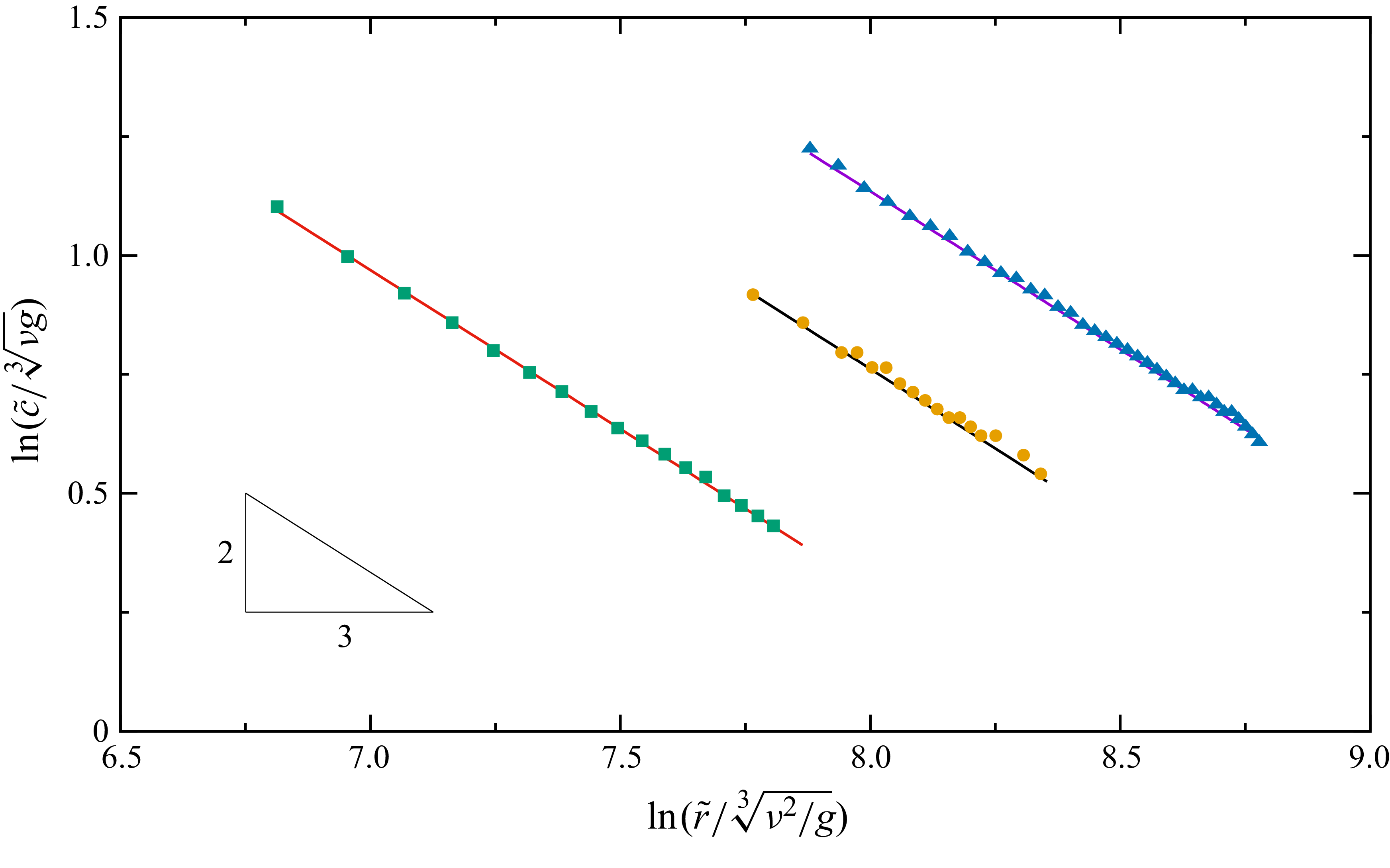
The lines in figure 4 show $c$ as functions of $\tilde r$ , computed with (3.22). The polar angle is $\tilde \beta = 150^\circ$ . The Kapitza number is ${Ka}_\perp = 242$ . From left to right, the dimensionless volumetric flow rates are $N_{q\perp } = 851.5$ , 1703 and 3000, respectively. The corresponding dimensionless disturbance angular frequencies, defined as $N_{\omega \perp } = \tilde \omega (\nu /g^2)^{1/3}$ , are 0.108, 0.128 and 0.148. A remarkable characteristic is that the lines are nearly straight with a slope of $-2/3$ in the logarithm coordinates. Indeed, inserting the leading-order part of (3.15) into (3.22) yields

(3.23) \begin{equation} c^{(0)} = \frac {3 q_s^{2/3}}{K r^{2/3} \sin \beta } \propto r^{-2/3}. \end{equation}

The leading-order wavelength can be calculated accordingly following $\lambda ^{(0)} = 2 \pi c^{(0)}/\omega$ , which shares the same power law. The value of $c^{(0)}$ is $3/5$ times the phase speed in Zollars (Reference Zollars1974) (equation VI-17), if the same scaling is used. This difference arises because the latter used $A$ instead of $\text{d}(Ar)/\text{d}r$ as the local wavenumber.

Figure 4.

Phase speed of linear waves versus distance from cone apex; $\tilde \beta = 150^\circ$ , ${Ka}_\perp = 242$ . Lines: (3.22); symbols: $h$ – $q$ model (§ 4). Squares: $N_{q\perp } = 851.5$ , $N_{\omega \perp } = 0.108$ ; circles: $N_{q\perp } = 1703$ , $N_{\omega \perp } = 0.128$ ; triangles: $N_{q\perp } = 3000$ , $N_{\omega \perp } = 0.148$ .

In addition, it would be useful to non-dimensionalise the phase speed with the Nusselt scaling (Kalliadasis et al. Reference Kalliadasis, Ruyer-Quil, Scheid and Velarde2012) and compare the results with the flat-plate situation. In that scaling, the characteristic velocity is chosen as $\tilde {h}_{N\mathrm{2D}}^2 /(l_\nu t_\nu )$ , where $ \tilde {h}_{N\mathrm{2D}}$ is the Nusselt film thickness defined in (1.1). The viscous-gravity length and time scales are $l_\nu =[\nu ^2/(g\sin \tilde \varphi )]^{1/3}$ and $t_\nu = [\nu /(g\sin \tilde \varphi )^2]^{1/3}$ , respectively. For the current conical scenario, we apply a modified Nusselt scaling by replacing $\tilde {h}_{N\mathrm{2D}}$ with the leading-order approximation to the local base-flow film thickness $\tilde h_{N\ell }$ , see (1.5). In this way, the velocity scale is written as $\tilde {h}_{N\ell }^2 / (l_\nu t_\nu )$ , with the length and time scales

(3.24) \begin{equation} l_\nu = \left ( \frac {\nu ^2}{-g \cos \tilde \beta } \right )^{1/3} \quad \mathrm{and} \quad t_\nu = \left ( \frac {\nu }{g^2 \cos ^2\tilde \beta } \right )^{1/3}, \end{equation}

respectively (the relation $\tilde \beta = \pi /2 + \tilde \varphi$ has been used). With this non-dimensionalisation, (3.23) yields a leading-order phase speed of

(3.25) \begin{equation} c^{\prime (0)} = \frac { \tilde c^{(0)} (\tilde r) l_\nu t_\nu }{ \tilde h^2_{N\ell } (\tilde r) } \equiv 1, \end{equation}

which is irrelevant to $\tilde r$ . This value is identical to the leading-order flat-plate result. The same conclusion, however, does not hold for the first- and second-order components, in which the present conical results contain $\tilde r$ -dependent terms. That being said, when taking $\tilde r \rightarrow \infty$ , the present expressions exactly reduce to the flat-plate ones obtained with spatial-mode stability analysis. In particular, the first-order correction is $\tilde c^{(1)}_{\mathrm{2D}} = 0$ , while the second-order component, in dimensional form, is

(3.26) \begin{equation} \tilde {c}^{(2)}_{\mathrm{2D}} = - \frac {2 \nu \tilde {\omega }^{2} \sin ^{2}\tilde {\beta }}{9 g \cos ^{3}\tilde {\beta }} + \frac {\nu \tilde {\omega }^{2}}{g \cos \tilde {\beta }} - \frac {2 \tilde {\omega }^{2} \tilde {Q}_{\mathrm{2D}} \sin \tilde {\beta }}{35 g \cos ^{2}\tilde {\beta }} + \frac {44 \tilde {\omega }^{2} \tilde {Q}_{\mathrm{2D}}^{2}}{175 g \nu \cos \tilde {\beta }}. \end{equation}

5.1. Morphology of surface waves

The instantaneous profiles in figure 7 reveal some important characteristics of the waves. Similar to the linear-theory prediction in § 3.2, the wavelength decreases with the distance from the cone apex. This is accompanied with the damping of the wave amplitude. The waves become shorter and weaker, eventually diminishing at large $\tilde r$ . This phenomenon is also consistent with the linear result in § 3, where it is shown that the film flow is stable at large radial distances, see figure 3. For small $\tilde r$ , the waves are solitary; as $\tilde r$ increases, a transition to sinusoidal-shaped waves is observed.

The contour map in figure 9 shows the spatio-temporal evolution of the waves for a representative case we have simulated. The film thickness is indicated by brightness, so that the wave peaks can be traced following the bright lines in the figure. The instantaneous shape of the free surface corresponding to $\tilde t = 0$ is presented on the bottom.

The phase speed of the waves, as can be deduced from the slopes of the bright lines in figure 9, is also a decreasing function of $\tilde r$ . This trend is also the same as that of linear waves, see figure 4. The more curved bright lines at smaller $\tilde r$ indicate larger decreasing rates of the phase speed. This is because the liquid film spreads out and thins more significantly due to the conical geometry in small- $\tilde r$ regions. At sufficiently large radial distance, the variation of flow characteristics with $\tilde r$ becomes mild; the film flow approaches the flat-plate limit described by (4.8) and (4.9).

For a more systematic examination, we conducted simulations with $\tilde \beta$ ranging from $100^\circ$ to $150^\circ$ with an increment of $5^\circ$ . The other parameters are set to ${Ka}_\perp = 242$ , $N_{q\perp } = 11242$ and $N_{\omega \perp } = 0.221$ . These values are selected to be moderate, allowing observation of different types of surface waves as $\tilde {\beta }$ is varied. Three representative cases are selected from the results with successively increasing angles $\tilde \beta = 110^\circ$ , $130^\circ$ and $150^\circ$ , see figure 10. The green dashed lines represent undisturbed free surfaces. Both the radial and cross-stream coordinates are non-dimensionalised by the film thickness $\tilde h_{\textit{in}}$ at the inlet. As can be seen, steeper cones produce larger wave amplitude near the axis, with more solitary waves observed before the waves become sinusoidal. The number of capillary ripples ahead of the main hump also increases (see insets). An interesting observation is that, although the steady-state film thickness decreases with $\tilde r$ , the envelop of the wave troughs is nearly parallel to the cone surface.

Figure 10.

Instantaneous wave profiles for $\tilde \beta = 110^\circ$ (a), $130^\circ$ (b) and $150^\circ$ (c). Here, ${Ka}_\perp = 242$ , $N_{q\perp } = 11242$ and $N_{\omega \perp } = 0.221$ . Dashed lines show undisturbed free surfaces obtained with the $h$ – $q$ model. The blue arrow in panel (c) marks the position of the turning point in figure 14. A depiction of $\tilde {\beta }$ is displayed in panel (a).

The phase speeds of the surface waves for the three cases shown in figure 10 are presented in figure 11(a). The symbols are extracted from the results of $h$ – $q$ model at discrete radial positions. The straight lines show the leading-order predictions from linear theory, (3.23), whose dimensional form reads

(5.1) \begin{equation} \tilde {c}^{(0)} = \left (\frac {3 \tilde {Q}}{2 \pi \tilde {r} \sin \tilde \beta }\right )^{2/3} \left (- \frac {g \cos \tilde \beta }{\nu }\right )^{1/3}. \end{equation}

Figure 11.

(a) Phase speed versus radial distance. Yellow, green and purple symbols represent the results of $h$ – $q$ model for cases in figure 10(a–c), respectively. Straight lines of the same colour display the leading-order phase speed predicted by linear theory. Vertical dashed lines mark positions where the normalised fundamental-frequency amplitude exceeds $90\,\%$ (§ 5.2). (b) Neutral curves of absolute (solid) and relative (dashed) growth. The colour scheme is the same as in panel (a). The horizontal dash-dotted line shows the disturbance angular frequency $N_{\omega \perp } = 0.221$ .

For all three cases, the phase speed agrees with the linear theory at sufficiently large $\tilde r$ , coinciding with the observation in figure 10 that the waves convert to small-amplitude linear waves eventually. In the region where $\tilde r$ is small, however, different behaviours are observed: the waves in figure 10(a) have more pronounced depression, with phase speeds smaller than the leading-order solution of linear waves. These are the characteristics of the $\gamma _1$ -type waves, or slow waves, defined by Chang et al. (Reference Chang, Demekhin and Kopelevich1993a , Reference Chang, Demekhin and Kopelevichb ). On the contrary, the waves close to the inlet in figure 10(c) are elevation dominant, with phase speeds larger than those of linear waves. These are $\gamma _2$ -type waves, or fast waves, according to Chang et al. (Reference Chang, Demekhin and Kopelevich1993a , Reference Chang, Demekhin and Kopelevichb ).

The occurrence of $\gamma _1$ and $\gamma _2$ waves in different cases can be interpreted with the neutral curves in figure 11(b), where the disturbance frequency for the cases in figure 10 is shown by the horizontal dash-dotted line. Liu et al. (Reference Liu, Paul and Gollub1993) found that, on a flat plate, $\gamma _1$ waves appear when the forcing frequency is just below the cutoff frequency; whereas $\gamma _2$ waves emerge at still lower frequencies. As illustrated in figure 11(b), at a given $\tilde r$ , the cutoff angular frequency $\tilde \omega$ increases with $\tilde \beta$ . Therefore, $\gamma _2$ waves are more likely to be observed when $\tilde \beta$ is large.

In the flat-plate situation, $\gamma _1$ waves are unstable (Kalliadasis et al. Reference Kalliadasis, Ruyer-Quil, Scheid and Velarde2012, p. 271) and easily switch to $\gamma _2$ waves in the presence of forced inlet disturbances (Liu & Gollub Reference Liu and Gollub1994). However, this secondary instability can be suppressed on a conical surface: figure 11(b) shows that, as $\tilde r$ increases, the range of unstable $\tilde \omega$ narrows. Therefore, disturbances capable of triggering the secondary instabilities may not have sufficient time to amplify before they are damped. Consequently, for small $\tilde \beta$ , the entire free surface can be dominated by $\gamma _1$ waves (figure 10 a), whereas for large $\tilde \beta$ , a transition from $\gamma _2$ to $\gamma _1$ waves may occur (figure 10(c), also see the purple lines and symbols in figure 11(a)).

5.2. Transition from solitary to sinusoidal waves

As shown in § 5.1, the surface waves undergo a transition from solitary to sinusoidal-like profiles. Considering the importance of wave shapes in pertinent heat- and mass-transfer processes (see, e.g. Miyara Reference Miyara1999, Reference Miyara2000a ; Aktershev et al. Reference Aktershev, Alekseenko and Tsvelodub2022), we elaborate on this transition in detail.

The top panels of figures 12(a–d) present the instantaneous film thickness versus time at four fixed downstream positions with $\tilde r/\tilde h_{\textit{in}}=200$ , 400, 500 and 700, respectively. The case is identical to that shown in figure 9, in which the four positions are indicated by vertical dashed lines. The bottom panels show the corresponding fast Fourier transform (FFT) spectra based on the periodic time series. The amplitudes are normalised by their sum for all non-zero frequency components. The red arrows mark the disturbance frequency imposed at the inlet. At $\tilde {r} / \tilde h_{\textit{in}} = 200$ , the waves are solitary, producing multiple spectral peaks in the FFT results. Further downstream, the wave shape smooths with fewer fluctuations in time. Correspondingly, the number of visible components in the FFT results decreases, with the fundamental frequency becoming more pronounced. At $\tilde {r} / \tilde h_{\textit{in}}=700$ , the temporary wave evolution is almost sinusoidal. The spectrum is dominated by the fundamental frequency, with most high-order harmonics diminishing.

Figure 12.

Top panels show temporal evolution of film thickness at four radial positions for the case in figure 9. From (a) to (d), $\tilde r/\tilde h_{\textit{in}}=200$ , 400, 500 and 700, respectively. Bottom panels: corresponding normalised spectra (direct-current component removed). Red arrows indicate frequency of imposed disturbance at inlet.

The transition from solitary to sinusoidal waves is found to exhibit a close correlation with the linear stability threshold. Figure 13 shows the neutral curves of absolute (solid lines) and relative (dashed lines) growth for cases with different apex angles and liquid properties. Symbols of the same colour mark the positions where the normalised fundamental spectral amplitude exceeds $90\,\%$ at given disturbance frequencies. As can be observed, all symbols roughly align with the neutral curve for relative growth, indicating that the position where sinusoidal waves appear on a conical surface – if a 90 %-amplitude criterion is employed – can be estimated by the position from which the flow becomes stable in the relative sense. Consequently, when other parameters are fixed, a higher forcing frequency promotes the transition from solitary to sinusoidal waves.

Figure 13.

Dimensionless disturbance angular frequency versus radial distance. Lines represent neutral curves for absolute (solid) and relative (dashed) growth from linear theory. Purple: $\tilde \beta =135^\circ$ , ${Ka}_\perp =3388$ , $N_{q\perp }=11507$ ; black: $\tilde \beta =135^\circ$ , ${Ka}_\perp =332$ , $N_{q\perp }=7762$ ; blue: $\tilde \beta =150^\circ$ , ${Ka}_\perp =332$ , $N_{q\perp }=6722$ . Symbols of the same colour mark the transition positions where the fundamental-frequency amplitude exceeds $90\,\%$ . A depiction of $\tilde {\beta }$ is also displayed.

In figure 11(a), the radial positions of the $90\,\%$ -amplitude threshold are indicated by short vertical dashed lines. Clearly, the phase speeds coincide with the linear predictions to the right of these dashed lines. Therefore, the solitary–sinusoidal-wave transition also signals the transition from nonlinear to linear waves. Indeed, the typical amplitude of the sinusoidal waves observed in our numerical simulations is as small as approximately $0.2 \,\%$ of the local wavelength.

Figure 14 shows the phase speed (a) and wave peak height (b) versus $\tilde r$ for the case in figure 10(c). The peak height is non-dimensionalised as $\tilde {h}_p / \tilde {h}_{N\ell } - 1$ , where $\tilde {h}_{N\ell }$ is the local Nusselt film thickness given by (1.5). For this representative case, the entire domain can be divided into three distinct regions that are characterised by presence of $\gamma _2$ , $\gamma _1$ and sinusoidal waves, respectively. The typical wave profiles in each region are displayed in the insets of panel (b). Near the inlet, the forcing frequency lies well below the local cutoff value. Here, $\gamma _2$ waves develop and travel downstream, with their phase speeds larger than the leading-order linear solution (dashed line in panel a). At a larger $\tilde r$ , the computed and linear phase speeds cross, signalling the transition from $\gamma _2$ to $\gamma _1$ waves. Further downstream, the $90\,\%$ -amplitude criterion divides the solitary and sinusoidal-wave regions. The position, based on the FFT result, is $\tilde {r} /\tilde h_{\textit{in}} \approx 1500$ . The linear theory predicts a relative-growth threshold of $\tilde {r} / \tilde h_{\textit{in}} \approx 1618$ . The relative error between the two values is less than $8\,\%$ .

Figure 14.

Phase speed (a) and wave peak height (b) versus radial distance for the case in figure 10(c). Dashed line in panel (a) shows leading-order phase speed from linear theory. Crosses in panel (b) show positions where the number of capillary ripples decreases. The black circle highlights the turning point of the curve. The insets show typical wave profiles in different regions.

During the entire evolution process, the capillary ripples preceding the main hump diminish successively. The positions where their number drops are marked by crosses in figure 14(b). Right after the last capillary wave disappears, the trend of the peak height variation experiences a sudden change at approximately $\tilde {r}/\tilde h_{\textit{in}}= 1086$ (black circle). This turning point is also marked in figure 10(c) (blue arrow). Figure 15 presents the normalised amplitude of the fundamental frequency as a function of $\tilde r$ . It experiences a significant shift around the turning point (dashed line), as indicated by the black arrow. Considering the correspondence between the fundamental-frequency amplitude and wave profiles, the turning point can be regarded as the onset of solitary-to-sinusoidal transition. This will be further evidenced in § 5.3.

Figure 15.

Normalised amplitude of the fundamental frequency versus radial distance for the case in figure 10(c). Vertical dashed line shows the position of turning point identified in figure 14(b).

5.3. Peak height and phase speed of surface waves

For nonlinear two-dimensional solitary waves on a falling liquid film along a vertical plate, Nosoko et al. (Reference Nosoko, Yoshimura, Nagata and Oyakawa1996) proposed empirical correlations for the wave peak height $\tilde h_p$ and phase speed $\tilde c$ , which are

(5.2) \begin{equation} N_{hp\perp } = 0.49 {Ka}_\perp ^{-0.132} N_{\lambda \perp }^{0.39} Re_{\mathrm{2D}\perp }^{0.46}, \end{equation}

and

(5.3) \begin{equation} N_{c\perp } = 1.13 {Ka}_\perp ^{-0.06} N_{\lambda \perp }^{0.31} Re_{\mathrm{2D}\perp }^{0.37}, \end{equation}

respectively. In (5.2) and (5.3), the vertical version of the viscous-gravity length and time scales mentioned earlier, $l_{\nu \perp } = (\nu ^2/g)^{1/3}$ and $t_{\nu \perp } = (\nu /g^2)^{1/3}$ , are employed for non-dimensionalisation, i.e.

(5.4) \begin{equation} N_{hp\perp } = \tilde {h}_p/l_{\nu \perp }, \quad N_{\lambda \perp } = \tilde {\lambda }/l_{\nu \perp }, \quad N_{c\perp } = \tilde {c} t_{\nu \perp }/ l_{\nu \perp } . \end{equation}

The Kapitza number ${Ka}_\perp = \sigma / ( \rho \nu ^{4/3} g^{1/3} )$ has been defined in § 3. The Reynolds number $Re_{\mathrm{2D}\perp }$ takes the form of (1.2) with $\tilde \varphi = \pi /2$ in this vertical-plate situation.

Equations (5.2) and (5.3) have shown good consistency with DNS results (see, e.g. Miyara Reference Miyara2000b ; Zhou & Prosperetti Reference Zhou and Prosperetti2020b ). To apply these correlations to the conical geometry, we (i) replace $g$ with its streamwise component $-g \cos \tilde \beta$ , so that $l_\nu$ and $t_\nu$ in (3.24) are used instead of $l_{\nu \perp }$ and $t_{\nu \perp }$ in (5.4), and ${Ka}_\perp$ is changed to ${Ka} = \sigma / [ \rho \nu ^{4/3} (-g\cos \tilde \beta )^{1/3} ]$ ; (ii) use the local Reynolds number $Re_\ell$ (1.6) instead of the constant $Re_{\mathrm{2D}}$ . This leads to

(5.5) \begin{equation} N_{hp} = 0.49 {Ka}^{-0.132} N_{\lambda }^{0.39} Re_\ell ^{0.46}, \end{equation}

and

(5.6) \begin{equation} N_{c} = 1.13 {Ka}^{-0.06} N_{\lambda }^{0.31} Re_\ell ^{0.37}. \end{equation}

Figure 16 compares (5.5) and (5.6) with the results of $h$ – $q$ model. The data are extracted at different discrete radial coordinates within the fully developed region, covering a relatively wide range of $N_{hp}$ and $N_{c}$ . In figure 16(a), the wave peak height $N_{hp}$ calculated with (5.5) agrees well with the numerical result, with the largest relative error less than $6\,\%$ . The consistency is also acceptable for the phase speed $N_c$ as shown in figure 16(b), especially in the high- $N_c$ region. According to figure 14(a), the waves in this region are solitary waves.

Figure 16.

Comparison of peak height (a) and phase speed (b) between the $h$ – $q$ model results and (5.5) and (5.6); ${Ka}_{\perp } = 240$ and $N_{\omega \perp } = 0.177$ for all cases. Purple squares: $N_{q\perp } = 12084$ , $\tilde \beta = 120^\circ$ ; green circles: $N_{q\perp } = 13954$ , $\tilde \beta = 135^\circ$ ; yellow triangles: $N_{q\perp } = 12084$ , $\tilde \beta = 150^\circ$ . The dashed diagonal lines represent the points where the values on the horizontal and vertical axes are equal. A depiction of $\tilde {\beta }$ is displayed in panel (a).

The slight discrepancy at low $N_c$ therefore arises partly because Nosoko et al.’s correlation was obtained in the solitary-wave regime whereas the phase speed in solitary and sinusoidal regions exhibits different behaviours (figure 11 a). A similar mismatch was also reported by Miyara (2000a) for high-frequency, non-solitary-wave cases. In addition, Nosoko et al.’s experiments were conducted for $14 \leqslant Re_\ell \leqslant 90$ , whereas the data in figure 16 fall in the range $Re_\ell \lesssim 15$ . In any case, it is convenient to refit (5.6) with the present numerical data. Since it has been shown in § 5.2 that the wave profiles before and after the turning point have difference trends, only the data before the turning point are used for fitting. The resultant correlation is

(5.7) \begin{equation} N_c = 0.9 {Ka}^{-0.052} N_\lambda ^{0.26} Re_\ell ^{0.58}. \end{equation}

In the comparison shown in figure 16, the wavelength $\tilde {\lambda } = \tilde {\lambda } (\tilde {r})$ is extracted from the numerical results by measuring the distance between two neighbouring wave peaks. This $\tilde {r}$ -dependent wavelength is unknown a prior in practice, which renders the correlations descriptive rather than predictive. Therefore, it is useful to replace the wavelength with the wave frequency, which is constant and known in the current scenario. We define $N_f = \tilde {f} t_\nu$ as the dimensionless forcing frequency. By using the relation $\tilde c(\tilde r) = \tilde f \tilde {\lambda }(\tilde r)$ , whose dimensionless form is $N_c = N_f N_\lambda$ , $N_\lambda$ in (5.7) can be eliminated. The result is

(5.8) \begin{equation} N_c = 0.87 {Ka}^{-0.07} N_f^{-0.35} Re_\ell ^{0.78}. \end{equation}

Accordingly, with (5.8), (5.5) can be rewritten as

(5.9) \begin{equation} N_{hp} = 0.46 {Ka}^{-0.16} N_f^{-0.53} Re_\ell ^{0.76}. \end{equation}

Since $Re_\ell \propto 1/\tilde r$ (see (1.6)), $N_c$ and $N_{hp}$ also decay with $\tilde r$ following $N_c \propto \tilde r^{-0.78}$ and $N_{hp} \propto \tilde r^{-0.76}$ .

Figure 17 shows the peak height (a) and phase speed (b) versus $\tilde r$ for four cases in log–log coordinates. Good agreement between the results of $h$ – $q$ model (symbols) and predictions of (5.8) and (5.9) (solid lines) is observed up to the turning points that can be easily located in the figures. The result of (5.1) is shown with dashed lines in figure 17(b). The $90\,\%$ -amplitude positions mentioned in § 5.2 are marked with short vertical dashed lines for each case. As in figure 11(a), the linear phase speed coincides well with the numerical results in the sinusoidal-wave region.

Figure 17.

Peak height (a) and phase speed (b) versus radial distance. Symbols: $h$ – $q$ model. Solid lines: (5.9) and (5.8). Blue inverted triangles: $\tilde \beta = 110^{\circ }$ , ${Ka}_{\perp } = 240$ , $N_{q\perp } = 8969$ , $N_{\omega \perp } = 0.177$ ; purple squares: $\tilde \beta = 120^{\circ }$ , ${Ka}_{\perp } = 240$ , $N_{q\perp } = 12084$ , $N_{\omega \perp } = 0.228$ ; green circles: $\tilde \beta = 140^{\circ }$ , ${Ka}_{\perp } = 242$ , $N_{q\perp } = 11242$ , $N_{\omega \perp } = 0.221$ ; red triangles: $\tilde \beta = 150^{\circ }$ , ${Ka}_{\perp } = 242$ , $N_{q\perp } = 11242$ , $N_{\omega \perp } = 0.221$ . Dash-dotted lines in panel (b) shows (5.1); vertical dashed lines mark positions where the fundamental-frequency amplitude exceeds $90\,\%$ , see § 5.2. A depiction of $\tilde {\beta }$ is displayed in panel (a).

In conclusion, the waves ahead of the turning point are solitary and carry preceding capillary ripple(s); their peak height and phase speed can be described by correlations (5.8) and (5.9). Beyond the $90\,\%$ -amplitude location, the waves are small amplitude and sinusoidal, and their phase speed can be estimated by linear theory. The waves between these two positions exhibit transient behaviour.

7.1. Validity range of the theory

Stemming from the long-wave assumption, both the linear stability analysis and the $h$ – $q$ model are expected to be valid for $\varepsilon =H/L \ll 1$ . As a conservative estimate, we set $H/L \lesssim 0.01$ . Replacing $L$ with the radial distance $\tilde {r}$ and $H$ with the local film thickness estimated using (1.5), one obtains an inequality for $\tilde {r}$ , whose solution reads

(7.1) \begin{equation} \tilde {r} \gtrsim 100^{3/4} \left (- \frac {3 \nu \tilde Q}{2 \pi g \sin \tilde \beta \cos \tilde \beta } \right )^{1/4}. \end{equation}

For all data shown in the present paper, the minimal radial distance where they are extracted is taken around the threshold predicted by (7.1). In figures 7(a) and 7(b), these thresholds for $\tilde r$ are indicated by vertical dashed lines.

Another assumption that is made during the derivation is the smallness of the Reynolds number, i.e. $Re \sim O(1)$ . However, comparisons with DNS (figure 7) and experimental results (figure 8) demonstrate that, the current $h$ – $q$ model works consistently well up to $Re \lesssim 10$ ; and major wave properties can still be captured at $Re \lesssim 100$ . Such good performance ‘beyond expectation’ has been richly documented for the $h$ – $q$ model families derived from the long-wave expansion in the flat-plate scenario.

7.2. A double- $\varepsilon$ expansion strategy

In the Navier–Stokes equations (2.1)–(2.3), there are two ways in which the radial distance $\tilde r$ is involved: it may appear alone (e.g. $\tilde r$ , $\tilde r^{-1}$ and $\tilde r^{-2}$ ) or in the denominator of partial derivatives (e.g. $\partial /\partial \tilde r$ and $\partial ^2/\partial \tilde r^2$ ). Strictly speaking, $\tilde {r}$ in the two scenarios should not be normalised using the same characteristic length: while an individual $\tilde {r}$ reflects the influence of the radial distance itself on the flow, the derivatives of physical quantities with respect to $\tilde {r}$ represent how quickly these quantities vary with $\tilde {r}$ . The length scale across which these variations occur is the local wavelength, yet is irrelevant to the absolute value of $\tilde r$ . Accordingly, an individual $\tilde {r}$ should be normalised by its own scale, whereas $\tilde {r}$ in the bottom of derivatives is more appropriate to be normalised using the wavelength. (An exception is the situation in which the independent variable $\tilde r$ appears in the numerator of the derivative, as the length scale for the change of $\tilde r$ is itself ( $L_1$ ), instead of the wavelength $L_2$ . For example, as is evident, $\partial \tilde r / \partial \tilde r$ should have the order $L_1/L_1 \sim O(1)$ instead of $L_1/L_2 \sim O(\varepsilon _2/\varepsilon _1)$ (see below for more details). Thus, care should be taken when dealing with terms such as $\partial \tilde \psi /\partial \tilde r \approx -\partial \tilde (\tilde h/ \tilde r)/\partial \tilde r$ , in which case the normalisation should be performed after expansion, i.e. after $\tilde r$ is removed from the numerator of the partial derivative.) Based on this consideration, the non-dimensionalisation and long-wave expansion of the Navier–Stokes equations can be refined as follows.

Let $L_1$ and $L_2$ denote the characteristic length scales for the radial distance and wavelength, respectively. Two, instead of one, small parameters can be defined as

(7.2) \begin{equation} \varepsilon _1 = \frac {H}{L_1} \ll 1 , \quad \text{and} \quad \varepsilon _2 = \frac {H}{L_2} \ll 1. \end{equation}

Since $|\tilde \psi | \approx \tilde h/ \tilde r$ , $\tilde \psi$ as well as $\tilde \alpha$ is of order $O(\varepsilon _1)$ . With $u =\tilde u/U$ and $v = \tilde v/V$ , the balance of continuity equation leads to $V/U \sim \varepsilon _2$ . Thus, the following scalings are adopted:

(7.3) \begin{equation} \tilde {r} = L_1 r, \quad \frac {\partial }{\partial \tilde {r}} = \frac {1}{L_2} \frac {\partial }{\partial r}, \quad \tilde {\alpha } = \varepsilon _1 \alpha , \quad \tilde {u} = U u, \quad \tilde {v} = \varepsilon _2 U v, \quad \tilde {t} = \frac {L_2 t}{U}, \quad \tilde {p} = \rho g H p. \end{equation}

On substitution, the dimensionless Navier–Stokes equations read

(7.4) \begin{align}&\qquad\qquad\qquad \frac {\partial u}{\partial r} + \frac {1}{r} \frac {\partial v}{\partial \alpha } + 2 \frac {\varepsilon _1}{\varepsilon _2} \frac {u}{r} + \varepsilon _1 \frac {v}{r} \cot \beta - \varepsilon _1^2 \frac {v}{r} \alpha \csc ^2\beta = 0, \end{align}

(7.5) \begin{align}& \varepsilon _2 {\textit{Re}} \frac {\partial u}{\partial t} + \varepsilon _2 {\textit{Re}} u \frac {\partial u}{\partial r} + \varepsilon _2 {\textit{Re}} \frac {v}{r} \frac {\partial u}{\partial \alpha } = -\cos \beta + \varepsilon _1 \alpha \sin \beta + \frac {1}{2} \varepsilon _1^2 \alpha ^2 \cos \beta - \varepsilon _2 \frac {\partial p}{\partial r} \nonumber\\ & + \varepsilon _1 \varepsilon _2 \frac {\partial ^2 u}{\partial r^2} + \varepsilon _1 \varepsilon _2 \frac {2}{r} \frac {\partial u}{\partial r} + \frac {1}{r^2} \frac {\partial ^2 u}{\partial \alpha ^2} + \varepsilon _1 \frac {\cot \beta }{r^2} \frac {\partial u}{\partial \alpha } - \varepsilon _1^2 \frac {\alpha \csc ^2\beta }{r^2} \frac {\partial u}{\partial \alpha } - \varepsilon _1^2 2 \frac {u}{r^2} - \varepsilon _1 \varepsilon _2 \frac {2}{r^2} \frac {\partial v}{\partial \alpha }, \end{align}

and

(7.6) \begin{equation} 0 = \sin \beta + \varepsilon _1 \alpha \cos \beta - \frac {1}{r} \frac {\partial p}{\partial \alpha } + \varepsilon _2 \frac {1}{r^2} \frac {\partial ^2 v}{\partial \alpha ^2} + \varepsilon _1 \frac {2}{r^2} \frac {\partial u}{\partial \alpha }. \end{equation}

The no-slip boundary condition at the wall is the same as (2.16). And the kinematic boundary condition at the free surface becomes

(7.7) \begin{equation} \frac {\partial h}{\partial t} - \frac {\varepsilon _1}{\varepsilon _2} \frac {h u}{r} + u \frac {\partial h}{\partial r} + v = 0. \end{equation}

The tangential- and normal-stress balances at the free surface are given by

(7.8) \begin{equation} \begin{aligned} & \frac {1}{r} \frac {\partial u}{\partial \alpha } = 2 \left ( \varepsilon _1 \frac {\partial u}{\partial r} - \varepsilon _1 \frac {u}{r} - \varepsilon _2 \frac {1}{r} \frac {\partial v}{\partial \alpha }\right ) \left (- \varepsilon _2 \frac {\partial h}{\partial r} + \varepsilon _1 \frac {h}{r}\right ) - \varepsilon _1\varepsilon _2 \left ( \frac {\partial v}{\partial r} + \frac {v}{r} \right )\!, \end{aligned} \end{equation}

and

(7.9) \begin{align} - p + 2 \left (\varepsilon _2 \frac {1}{r} \frac {\partial v}{\partial \alpha } + \varepsilon _1 \frac {u}{r}\right ) = \left (\frac {\varepsilon _2}{\textit{Bo}}\right ) \mathcal{C},\end{align}

respectively, where the curvature $\mathcal{C}$ is

(7.10) \begin{equation} \mathcal{C} = \frac {\varepsilon _1}{\varepsilon _2} \frac {1}{r} \cot \beta + \frac {\varepsilon _1^2}{\varepsilon _2} \frac {h}{r^2} \cot ^2\beta + \varepsilon _1 \frac {1}{r} \frac {\partial h}{\partial r} + \varepsilon _2 \frac {\partial ^2 h}{\partial r^2}. \end{equation}

It is worthwhile to note that, when $\varepsilon _1 \sim \varepsilon _2 \sim \varepsilon$ , which corresponds to regions not too far from the cone apex, (7.4)–(7.10) reduce to (2.13)–(2.20). Whereas for positions at which the radial distance is much larger than the local wavelength, i.e. $\varepsilon _1 \ll \varepsilon _2$ , the effect of $\varepsilon _1$ terms in (7.4)–(7.10) diminishes or even vanishes in the present second-order framework. In such a scenario, (2.13)–(2.20) actually contain extra high-order (higher than second order) $\varepsilon _1$ terms, representing a more conservative approximation.

With the above preparations, we are able to examine the impact of different terms in the expression of curvature, (7.10). In this equation, the first term is the lateral curvature whose order is $O(\varepsilon _1/\varepsilon _2)$ . The last three terms represent the contribution of the streamwise curvature, with their orders of magnitude being $O(\varepsilon _1^2/\varepsilon _2)$ , $O(\varepsilon _1)$ and $O(\varepsilon _2)$ , respectively. If $\varepsilon _1 \sim \varepsilon _2$ , the lateral curvature is dominant. However, as $\tilde r$ increases (thus $\varepsilon _1$ decreases), its influence weakens, rendering the last term of the streamwise curvature pronounced. In other words, the present double- $\varepsilon$ expansion approach reveals that the lateral curvature is a dominant quantity only in the region close to the apex. It degrades to higher orders as $\tilde r$ increases. Physically speaking, this behaviour reflects the vanishing effect of cone surface curvature far from the apex.