INTRODUCTION
Seamounts are undersea mountains which rise from the ocean bottom to more than 1000 m without breaking through the sea level. They are usually of volcanic or tectonic origin and generally of conical shape with a circular, elliptical or elongated base (Rogers, Reference Rogers1994). In contrast to the surrounding flat sediment-covered abyssal plains seamounts feature different habitats of hard substrata or soft bottom. Some seamounts have a rugged, steeply sloping rocky bottom, while other wide seamounts are covered with sediment (Genin, Reference Genin2004).
Seamounts occur in chains, clusters or as isolated mountains (Menard, Reference Menard1964) and may have complex effects on ocean circulation and on the surrounding water body, depending on their size and shape (Rogers, Reference Rogers1994). One effect of the current–topography interaction is the production of jets and eddies (Vastano & Warren, Reference Vastano and Warren1976; Roden, Reference Roden1991). Eddies may be trapped over seamounts and form closed anticyclonic circulation cells known as a Taylor column (Roden, Reference Roden1991; White & Mohn, Reference White and Mohn2005). Taylor columns may have an impact on the intensity of advection and the retention of particles and plankton above the seamount and could be responsible for aggregations of zooplankton, micronekton and fish at seamounts (Genin & Boehlert, Reference Genin and Boehlert1985; Genin, Reference Genin2004) as well as changes in the pelagic food chain. Other possible hypotheses for increased stocks of organisms at seamounts include enhanced primary production caused by upwelling mechanisms or a stabilization of the water column (Dower et al., Reference Dower, Freeland and Juniper1992) as well as trapping of vertically migrating zooplankton which can be utilized by benthopelagic and epibenthic predators at the seamount summit (Genin et al., Reference Genin, Haury and Greenblatt1988, Reference Genin, Greene, Haury, Wiebe, Gal, Kaartvedt, Meir, Fey and Dawson1994; Dower & Mackas, Reference Dower and Mackass1996; Haury et al., Reference Haury, Fey, Newland and Genin2000).
In recent years several studies have been conducted at oceanic seamounts in the North Atlantic with the objective of understanding the hydrographical, biogeochemical and biological processes which govern the seamount ecosystem, especially at the Great Meteor Seamount and in the region of the Horseshoe Seamounts chain between Portugal and the Azores. In the Mediterranean Sea, where most seamounts are located in the Tyrrhenian Sea in the western basin, biological information about seamount ecosystems is scarce. In the eastern Mediterranean there are only very few seamount-like structures. The Anaximander Mountains arise south of Antalya in the northern Levantine Basin between the Cyprus Arc and the Hellenistic Arc. Whereas some of the numerous mud volcanoes resulting from tectonic activity around the Anaximander Mountains have been investigated for gas emanations and microbial activities, the pelagic and benthic fauna of these undersea mountains has not been described yet.
The seamounts in the eastern Mediterranean are fairly isolated from the world ocean and are located in a region with exceptionally high temperatures of the deep-water layers. Due to the semi-enclosed nature of the eastern Mediterranean in an arid region as well as a high evaporation rate and little freshwater input, salinity and temperature of the deep-water layers increase in the Mediterranean Sea from west to east (Hofrichter, Reference Hofrichter2002). In contrast to the typical salinity of 35 psu in the Atlantic and temperatures of 4–2°C below 1000 m (Angel & de C. Baker, Reference Angel and de C. Baker1982), the water of the Ionian and Levantine Basins shows a salinity of 38–39 psu and below 750 m a constant temperature of 13–14°C. The anti-estuarine water mass circulation as well as little nutrient input by rivers or the atmosphere in the Mediterranean Sea leads to a decrease in productivity from the Strait of Gibraltar in the west to the Asia Minor coast in the east (Turley, Reference Turley1999), with phytoplankton production up to three times lower in the eastern than in the western basin (Turley et al., Reference Turley, Bianchi, Christaki, Conan, Harris, Psarra, Ruddy, Stutt, Tselepides and v. Wambecke2000). The eastern Mediterranean is extremely nutrient-poor and is regarded as an oligo- to ultraoligotrophic region (Dugdale & Wilkerson, Reference Dugdale and Wilkerson1988). In this environment the deep Mediterranean waters are also poor in zooplankton abundance and diversity compared to the open ocean (Scotto di Carlo et al., Reference Scotto di Carlo, Ianora, Mazzochi and Scardi1991).
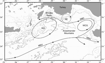
The circulation in the eastern Mediterranean is characterized by the occurrence of sub-basin and mesoscale cyclonic and anticyclonic eddies and gyres as well as permanent jets. The three major circulation features in the north-western Levantine Basin are the Rhodes gyre and two meandering currents, the Mid-Mediterranean Jet (MMJ) and the Asia Minor Current (AMC) (Figure 1). The MMJ flows through the central Levantine towards Cyprus where it bifurcates and one branch flows northward to feed the AMC (Robinson et al., Reference Robinson, Leslie, Theocharis, Lascaratos, Steele, Thorpe and Turekian2001), which is flowing westward along the Asia Minor coast. The stationary cyclonic Rhodes gyre between Rhodes and Cyprus is present throughout the year (Malanotte-Rizzoli & Bergamasco, Reference Malanotte-Rizzoli and Bergamasco1989, Reference Malanotte-Rizzoli and Bergamasco1991; Robinson et al., Reference Robinson, Golnaraghi, Leslie, Artegiani, Hecht, Lazzoni, Michelato, Sansone, Theocharis and Ünlüata1991). A persistent anticyclonic feature, the Anaximander eddy, is located between the Rhodes gyre and the Anatolian coast, where it appears to be locked on to the Anaximander Seamounts (Özsoy et al., Reference Özsoy, Hecht, Ünlüata, Brenner, Oguz, Bishop, Latif and Rozentraub1991, Reference Özsoy, Hecht, Ünlüata, Brenner, Sur, Bishop, Latif, Rozentraub and Oguz1993; Theocharis et al., Reference Theocharis, Georgopoulos, Lascaratos and Nittis1993).
Surface circulation in the northern Levantine Basin of the eastern Mediterranean: the Rhodes Basin and the Anaximander Mountains. RG, Rhodes gyre; AE, Anaximander eddy; WCG, West Cyprus gyre; MMJ, Mid-Mediterranean Jet; AMC, Asia Minor Current (figure not to scale; modified after Malanotte-Rizzoli & Bergamasco, Reference Malanotte-Rizzoli and Bergamasco1991; Özsoy et al., Reference Özsoy, Hecht, Ünlüata, Brenner, Oguz, Bishop, Latif and Rozentraub1991; Robinson et al., Reference Robinson, Golnaraghi, Leslie, Artegiani, Hecht, Lazzoni, Michelato, Sansone, Theocharis and Ünlüata1991).

The primary goal of cruise M71/1 of RV ‘Meteor’ to one peak (Anaximenes Mountain) of the Anaximander Mountains in the northern Levantine Basin of the eastern Mediterranean was to assess the ecosystem of a seamount in an oligotrophic region with a warm deep-water body, including studies of the surrounding nutrient and current regime and the impact of the seamount on the surrounding ocean. This study focuses on the question, how the seamount affects the biomass, abundance, vertical distribution, taxonomic composition and trophic structure of the zooplankton community in an oligotrophic region, as compared to the open water column of the Rhodes Basin. In this context the following main questions are addressed:
(1) Is the zooplankton biomass and abundance locally increased at the seamount? This is a phenomenon often found at seamounts and attributed to the interaction of the topography with the current regime. Based on the depth of the summit and the surrounding flow field we assume that a retention effect or enhancement of productivity at the seamount will only be weak.
(2) Does the size distribution of zooplankton above the seamount summit differ from the slope and the Rhodes Basin? Based on results from seamounts in the north-east Atlantic, the assumption is made that the zooplankton above the summit is mainly composed of smaller taxa while organisms >5 mm are rarely represented. The reasons for this are not quite clear, but predation by seamount-associated pelagic or benthopelagic fauna may play a role.
(3) Do the possible seamount effects on the plankton community lead to differences in the food web structure between seamount and reference station, and is this mirrored in the stable isotope signatures? Usually an enrichment of 15N and 13C in zooplankton organisms with increasing size and increasing depth can be observed, indicating the length of the food chain. Differences in the distribution of the stable isotope ratios would point to differing food availability at the sampling locations.
MATERIALS AND METHODS
Study regions
Zooplankton was sampled in the Rhodes Basin and at the Anaximander Mountains in the northern Levantine Basin of the eastern Mediterranean (Figure 1) during cruise M71/1 of RV ‘Meteor’ in December 2006. The sampling site in the Rhodes Basin was situated south-east off Rhodes at 35°50 N 28°75E. Water depth was about 4500 m above a flat sedimentary plain. The Anaximander Mountains are located south of Antalya ~54 noutical miles off the Turkish coast and comprise three elevations which rise more than 1000 m above the surrounding seafloor, Anaximander to the west, Anaximenes in the centre and Anaxagoras to the east. The Anaximander Mountains feature areas with steep rocky slopes as well as gently-sloping sedimentary regions. Water depth at the base is about 2000 m, and the minimum summit depth is ~800 m at the Anaximenes Mountain, which forms an elongated elevation without a wide summit plateau. In the north-eastern direction the Anaximenes is separated from the Anaxagoras Mountain by a saddle region of 1600 m water depth.
Zooplankton sampling and sample processing
ZOOPLANKTON SAMPLES
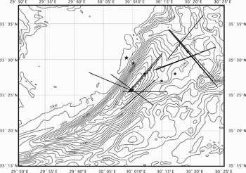
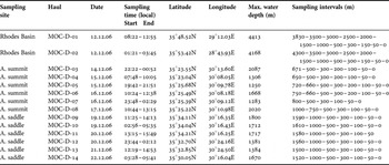
Zooplankton was caught by oblique hauls with a 1m2-Double-MOCNESS (Multiple Opening and Closing Net and Environmental Sensing System; Wiebe et al., Reference Wiebe, Morton, Bradley, Backus, Craddock, Barber, Cowles and Flierl1985). At all sampling sites, the whole water column subdivided into smaller sampling intervals, was sampled from a few metres above the bottom to the surface (Table 1). The towing speed was 2 knots. The MOCNESS was equipped with 20 nets of 333 µm mesh size as well as a bathometer, a clinometer, a flowmeter and sensors for temperature and salinity. Environmental data (temperature, salinity, conductivity and pressure) were recorded simultaneously during sampling. In the Rhodes Basin, one day and one night profile for zooplankton were sampled. In the Anaximander Mountains region, zooplankton samples were taken both above the summit of the Anaximenes and in the saddle region between Anaximenes and Anaxagoras three times at day and three times at night (Figure 2). All station and sampling data are presented in Table 1.
MOCNESS-tracks (lines) und CTD-rosette-stations (*) at the Anaximenes Mountain (bathymetry after ten Veen et al., Reference ten Veen, Woodside, Zitter, Dumont, Mascle and Volkonskaia2004).

Zooplankton sampling data.

Max., maximum; A, Anaximenes.
Upon recovery of the MOCNESS, the nets were rinsed with seawater. One half of the zooplankton samples were preserved in 4% formaldehyde–seawater solution buffered with borax for biomass determination and taxonomic identifications. The other half of the material was rinsed with freshwater and fractionated by sieving into the size-classes <0.5 mm, 0.5–5 mm and >5 mm for the analysis of stable nitrogen and carbon isotopes. The following taxa were withdrawn from the fractionated samples and processed separately: Pisces, Chaetognatha, Decapoda, Eucalanus spp., Haloptilus spp. and Lucicutia spp. All material was frozen at –20°C and later dry-frozen at –40°C and pulverized for further analyses.
In the laboratory, the zooplankton samples preserved in formaldehyde were fractionated by sieving into the size-classes <0.5 mm, 0.5–1 mm, 1–2 mm, 2–5 mm and >5 mm. The wet weight of each size fraction was measured after removal of the interstitial water with 70% alcohol according to the method of Tranter (Reference Tranter1962). Wet weights were used to allow for subsequent taxonomic identification of the sample. The fractionated zooplankton was sorted into its main groups. Carcasses, according to Wheeler (Reference Wheeler1967) and Weikert (Reference Weikert1977), were counted separately, also fragments of gelatinous organisms like Siphonophora. The Copepoda were identified at the family or genus level, abundant taxa of them at the species level. Only both catches of the Rhodes Basin and in each case two day and two night catches each of the seamount summit and of the saddle region were analysed taxonomically.
Biomass (wet weight) was standardized to milligrams per 1000 m3 (10−3 mg m−3) and abundances to individuals per 1000 m3 (10−3 ind m−3). Standing stocks in terms of biomass and abundance for the whole water column or a given depth-range were calculated as mg m−2 and ind m−2, respectively. For the statistical analysis, data were log-transformed [Y′ = ln(Y + 1)] in order to reach approximate normal distribution and homogeneity of variances. One- and two-way analyses of variance (ANOVAs) (Clarke, Reference Clarke1993; Lozán & Kausch, Reference Lozán and Kausch2004) were used to test for differences between zooplankton standing stocks of the Rhodes Basin and the Anaximenes Mountain. Differences in the vertical distribution of zooplankton size-fractions were tested at the seamount summit and saddle; the Rhodes Basin was not included in these tests because data were only available from one day and one night haul.
POM SAMPLES
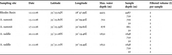
Additionally water samples for the determination of stable isotope ratios of suspended particulate organic matter (POM) were taken by a CTD (conductivity–temperature–depth)-rosette in different water depths at each zooplankton sampling location (Table 2). In the Rhodes Basin water samples from 4425 m, 750 m and 50 m depth were used for the analysis of POM. At the Anaximenes Mountain, seston samples were taken at 702 m, 678 m and 50 m above the summit and at depths of 1650 m, 750 m and 50 m in the saddle region.
Water sampling data.
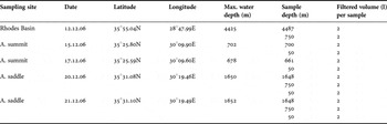
Max., maximum; A, Anaximenes.
For further analyses of stable isotope ratios of POM 3 × 2 l of each water sample were filtrated on precombusted fibre glass filters (Whatman GFC, diameter 2.5 cm, pore size 1.2 µm) and frozen at –20°C on board. The stable isotope composition of POM was determined according to the method described below.
MEASUREMENT OF δ15N AND δ13C
The analyses of nitrogen (δ15N) and carbon isotope ratios (δ13C) were done at the Humboldt-University of Berlin by the working group of Professor U. Struck, Museum of Natural History. Measurements of N- and C-isotope ratios of zooplankton and POM were made with an isotope-ratio mass-spectrometer (Thermo Finnigan Delta V) with a connected upstream of an elementar analyser (Thermo EA-1112 CHN-Analyser). The analytical error of this method is <0.2‰ (Struck et al., Reference Struck, Emeis, Voß, Krom and Rau2001). Stable isotopes values are expressed in δ notations as parts per thousand (‰):

where Rsample is the ratio of 15N/14N and 13C/12C, respectively, of the particular sample, and Rstandard is the N-isotope ratio of atmospheric nitrogen and the C-isotope ratio of the fossil Cephalopoda (Belemnitella americana), respectively.
Stable isotope ratios of POM and zooplankton were tested statistically by a one-way ANOVA for differences in each case between the three locations and between different depth layers. A model without interactions had to be chosen because some cells showed only single values. Data approximately showed normal distribution and homogeneity of variances.
RESULTS
Hydrography
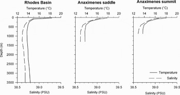
Surface water temperatures ranged between 17.8 and 18.3°C, building a warm surface layer in the upper 50 m with salinity values of 39.0–39.2 psu. At the Anaximenes Mountain temperature and salinity continuously decreased to ~13.9°C and 38.6 psu at 500 m, remaining rather constant below this depth (Figure 3). In the Rhodes Basin surface temperature and salinity showed an abrupt decrease to 15.0°C and 38.8 psu at 100 m before they continuously decreased to 13.9°C and 38.6 psu at 500 m. Down to 4000 m values remained constant.
Vertical profile of temperature and salinity in the Rhodes Basin and at Anaximenes saddle and summit.

Distribution of zooplankton biomass and abundance
ZOOPLANKTON STANDING STOCK IN THE UPPER 1000 M
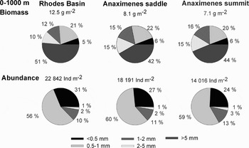
The standing stocks of zooplankton in the upper 1000 m were measured in order to compare the occurrence of zooplankton at sampling sites of different depth. Highest standing stocks of biomass were found in the Rhodes Basin (12.0–12.9 g m−2). Lowest standing stocks appeared above the seamount summit (5.32–8.18 g m−2) (Figure 4).
Mean standing stocks of zooplankton biomass (g m−2) and abundance (ind m−2) and the percentage contribution of five size-classes in the upper 1000 m in the Rhodes Basin and at Anaximenes saddle and summit (mean values of day and night catches).

The highest standing stock in term of abundance in the upper 1000 m occurred during the night in the Rhodes Basin (33,600 ind m−2). Standing stocks at the Anaximenes Mountain ranged between highest values of 20,900 ind m−2 in the saddle region and lowest values of 12,000 ind m−2 above the summit (Figure 4). At all three sampling sites, standing stocks of biomass and abundance in the upper 1000 m were higher at night than at daytime, but not significantly as an ANOVA showed.
The size composition of zooplankton was similar at all sampling sites (Figure 4). The smallest size fraction (<0.5 mm) contributed only 5–6% to the total zooplankton biomass, but made up 24–31% of all individuals. The size-class 0.5–1 mm was numerically most abundant, contributing 56–60% to the total zooplankton. In terms of biomass, their share was 20–22%. The size-class 1–2 mm reached 12–16% in terms of biomass and 10–13% in terms of abundance; the share of size-class 2–5 mm was 10–15% and 2–3%, respectively. Although the largest size-class (>5 mm) contributed only 1% to all individuals, in terms of biomass they made up nearly half of the total standing stock.
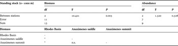
An ANOVA of pooled day and night data indicates a significantly higher biomass standing stock in the Rhodes Basin than at the Anaximenes Mountain (Table 3), but no difference between standing stocks at the seamount summit and the saddle region was detected. The standing stocks of zooplankton abundance did not differ significantly between the Rhodes Basin and the seamount region.
One-way-ANOVA of differences in biomass and abundance standing stock (0–1000 m) between Rhodes Basin, Anaximenes summit and Anaximenes saddle, and matrix of pairwise comparisons after Bonferroni comparisons.

df, degrees of freedom; F, F ratio of mean squares; P, probability of correlation; *, P < 0.05; n.s., P > 0.05.
VERTICAL DISTRIBUTION OF ZOOPLANKTON BIOMASS AND ABUNDANCE
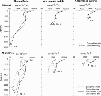
Highest concentrations of zooplankton (biomass and abundance) occurred in the epipelagic zone in the upper 100 m at all sampling sites (Figure 5). Biomass concentration at this depth ranged between 50 × 10−3g m−3 during night in the Rhodes Basin and 19 × 10−3g m−3 at daytime above the seamount summit. Abundance showed the same distribution pattern: highest numbers of 200,000 × 10−3ind m−3 were found during night in the Rhodes Basin while lowest numbers of 75,000 × 10−3ind m−3 occurred at day above the seamount summit.
Vertical distribution of living zooplankton biomass (mg 10−3m−3) and abundance (ind 10−3m−3) and of exoskeleton abundance in the whole sampled water column during day and night in the Rhodes Basin and at Anaximenes saddle and summit. N, number of hauls (mean values at seamount); horizontal lines, range between minimal and maximal values.

Below 100 m, concentrations generally decreased with depth; however, a second maximum of biomass concentration occurred at 750 m at all sampling sites, during the day as well as during the night. This pattern was less clear in the abundance estimates: in the Rhodes Basin, elevated abundances were found at 750 m in the night haul, but not during the day. In the Anaximenes saddle region neither the day hauls nor the night hauls indicated higher abundances at 750 m. Above the summit, abundances varied only slightly below 400 m, increasing weakly during night.
Only in the Rhodes Basin the water column reaches into the bathypelagic zone, where biomass concentration and numbers of individuals decreased between 1000 and 3000 m from 5.6 × 10⁻³g m−3 to 0.11 × 10⁻³g m−3 and from 3800 × 10−3ind m−3 to 23 × 10−3ind m−3 (mean values), respectively. Below 3000 m a slight increase to 0.29 × 10⁻³g m−3 and 320 × 10−3ind m−3 was observed.
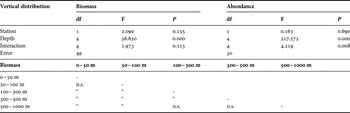
The vertical distributions of zooplankton biomass and abundance (of pooled day and night data) in the Anaximenes Mountain region were tested for differences between stations and depths. A two-way ANOVA indicates significant differences in biomass between depth layers, but not between the two locations saddle and summit (Table 4). The subsequent Bonferroni comparisons confirm the strong decrease below 100 m. The two-way ANOVA for the abundance shows a highly significant interaction term, indicating differences in the vertical distribution patterns between the two locations.
Two-way-ANOVA between factors station (Anaximenes saddle and summit) and depth for zooplankton biomass and abundance, and matrix of pairwise comparisons after Bonferroni comparisons for vertical differences of zooplankton biomass.

df, degrees of freedom; F, F ratio of mean squares; P, probability of correlation; *, P < 0.05; n.s., P > 0.05.
VERTICAL DISTRIBUTION OF EXOSKELETON ABUNDANCE
Figure 5 shows the vertical distribution of exoskeleton abundance in relation to living zooplankton. Exoskeletons were found throughout the water column at all sites. Numbers of exoskeletons were highest in the upper 100 m and decreased towards the bottom, while the relative amount of exoskeletons to living zooplankton was lowest in the upper 100 m, by trend increasing with increasing depth.
In the epipelagic zone numbers of exoskeletons ranged between 26,900 × 10−3ind m−3 in the Rhodes Basin and 4900 × 10−3ind m−3 above the seamount summit during night. Between 150 and 1000 m exoskeleton numbers remained constant in the Rhodes Basin, while they decreased generally towards the bottom in the seamount region. In the bathypelagic zone of the Rhodes Basin, a second maximum of exoskeletons occurred between 1000 and 1500 m. Towards 3000 m depth exoskeleton numbers decreased to a minimum value (34 × 10−3ind m−3) and showed again a slight increase below this depth.
The relative amount of exoskeletons to living zooplankton was 7% in the upper 100 m of the Rhodes Basin and 2–5% in the seamount region. An increase with increasing depth was observed, showing in the Rhodes Basin a first peak between 1000 and 1500 m (88%) and a second peak between 2500 and 3000 m (149%). Below 3500 m exoskeletons made up 247% relative to the living zooplankton. Above the seamount summit and in the saddle region the relative amount of exoskeletons to living zooplankton during night was highest between 300 and 500 m (13–16%), whereas during day the amount was highest below 500 m, ranging between 17% above the summit and 37–74% in the saddle region.
VERTICAL DISTRIBUTION OF ZOOPLANKTON AND ABUNDANCE OF DIFFERENT SIZE-CLASSES
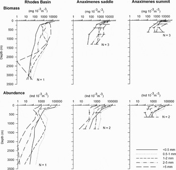
At all sites the biomass of organisms <0.5 mm decreased from the surface towards the bottom. Biomass concentrations of the size-groups >0.5 mm were also highest in the upper 100 m, but a secondary peak occurred in intermediate depths between 500 and 1500 m.
Highest numbers of individuals were counted at all depths for the size-class 0.5–1 mm, lowest numbers for the class >5 mm, in the Rhodes Basin as well as in the Anaximenes Mountain region. The abundance of zooplankton <0.5 mm decreased from the surface towards the bottom, like the biomass. Between 500 and 2500 m the abundance of organisms >1 mm proportionally increased. In the Rhodes Basin individual numbers of all size fractions showed again a slight increase below 3000 m (Figure 6).
Vertical distribution of biomass (mg 10−3m−3) and abundance (ind 10−3m−3) of different zooplankton size-classes in the whole sampled water column during night in the Rhodes Basin and at Anaximenes saddle and summit. N, number of hauls (mean values at seamount); horizontal lines, range between minimal and maximal values.

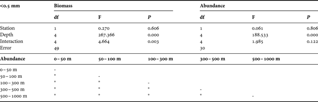
The vertical distribution of biomass and abundance of every size-class in the Anaximenes Mountain region were tested for differences between stations and depths (two-way-ANOVA; Tables 5–9). Day and night data were pooled for each size-class, because there were no significant differences detectable between day and night distributions by ANOVA.
Zooplankton size-class <0.5 mm: two-way-ANOVA between factors station (Anaximenes saddle and summit) and depth for (a) biomass and (b) abundance, and matrix of pairwise comparisons after Bonferroni comparisons for vertical differences of zooplankton abundance.
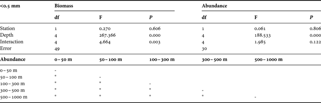
df, degrees of freedom; F, F ratio of mean squares; P, probability of correlation; *, P < 0.05; n.s., P > 0.05
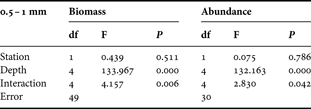
Zooplankton size-class 0.5–1 mm: two-way-ANOVA between factors station (Anaximenes saddle and summit) and depth for (a) biomass and (b) abundance.
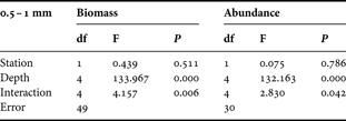
df, degrees of freedom; F, F ratio of mean squares; P, probability of correlation.
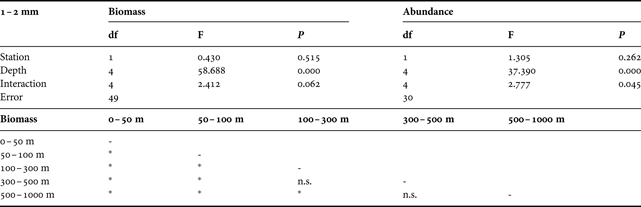
Zooplankton size-class 1–2 mm: two-way-ANOVA between factors station (Anaximenes saddle and summit) and depth for (a) biomass and (b) abundance, and matrix of airwise comparisons after Bonferroni comparisons for vertical differences of zooplankton biomass.
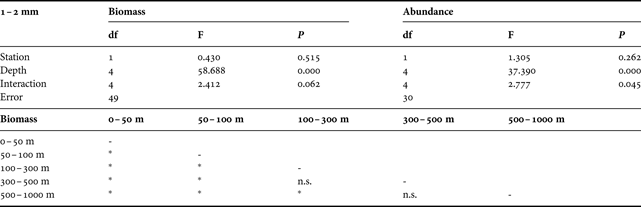
df, degrees of freedom; F, F ratio of mean squares; P, probability of correlation; *, P < 0.05; n.s., P > 0.05
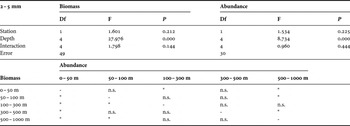
Zooplankton size-class 2–5 mm: two-way-ANOVA between factors station (Anaximenes saddle and summit) and depth for (a) biomass and (b) abundance, and matrix of pairwise comparisons after Bonferroni comparisons for vertical differences (lower half: biomass; upper half: abundance).

df, degrees of freedom; F, F ratio of mean squares; P, probability of correlation; *, P < 0.05; n.s., P > 0.05.
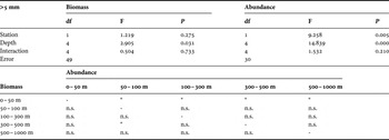
Zooplankton size-class >5 mm: two-way-ANOVA between factors station (Anaximenes saddle and summit) and depth for (a) biomass and (b) abundance, and matrix of pairwise comparisons after Bonferroni comparisons for vertical differences (lower half: biomass; upper half: abundance).

df, degrees of freedom; F, F ratio of mean squares; P, probability of correlation; *, P < 0.05; n.s., P > 0.05.
The ANOVAs for the biomasses of the size-classes <0.5 mm and 0.5–1 mm (Tables 5–6) show a highly significant interaction term in each case, indicating differences in the vertical distribution patterns between the two locations saddle and summit. The size fractions >1 mm show significant differences in biomass between depth layers, but not between the two locations (Tables 7–9). In case of the size fraction 1–2 mm, the Bonferroni comparisons verify the decrease of biomass especially in the upper 500 m. The decrease in biomass of the size fraction 2–5 mm from the surface to 300 m depth and below 500 m is also confirmed by the Bonferroni comparisons. The biomass of organisms >5 mm decreased strongly between 50 m and 500 m, as the Bonferroni test showed.
The ANOVAs for the abundance of the size-classes 0.5–1 mm and 1–2 mm (Tables 6–7) show a weakly significant interaction term in each case, pointing to differences in the vertical distribution patterns between the two locations saddle and summit. The ANOVA for the size fractions <0.5 mm and 2–5 mm (Tables 5–8) indicates significant differences in abundance between depth layers, but not between the two locations. The Bonferroni comparisons reflect the strong decrease of the abundance of organisms <0.5 mm from the surface towards the bottom as well as the decrease of the size fraction 2–5 mm within the upper 300 m and below 500 m. The two-way ANOVA for the abundance of organisms >5 mm (Table 9) indicates significant differences between the depth layers as well as between the two locations saddle and summit. In the upper 50 m individual numbers were much higher in contrast to greater depth layers, as the Bonferroni comparisons confirm. Between 100 and 300 m individual numbers were significantly higher above the summit than in the saddle region. In other depth layers significant differences were not detectable.
Zooplankton composition and distribution of the major taxonomic groups
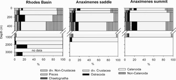
Zooplankton was sorted in the following seven major taxonomic groups: diverse Non-Crustacea, Pisces, Chaetognatha, diverse Crustacea, Ostracoda, Copepoda Calanoida and Copepoda Non-Calanoida. The group diverse Non-Crustacea includes Cnidaria, Tunicata, Mollusca, Polychaeta and diverse larvae. Diverse Crustacea include the groups Hyperiida, Gammarida, Malacostraca, Cladocera and Crustacea larvae.
Calanoida were generally the most numerous organisms in the whole water column at all sampling sites (Figure 7). Non-Calanoida ranked next with 12–33%. Depending on the depth, Calanoida made up 50–95% of the total zooplankton standing stock, reaching the highest relative portion between 500 and 1500 m. The lowest share of Calanoida (50–57%) occurred between 300 and 500 m. In this depth highest amounts of Non-Calanoida were detected. Below 500 m Non-Calanoida were less important for the taxonomic composition. Depending on the depth, Ostracoda contributed 1–20% with a maximum share between 100 and 500 m and a second peak below 2000 m. Diverse Crustacea and Non-Crustacea as well as Chaetognatha and Pisces contributed each ≤10% to the zooplankton standing stock. Chaetognatha occurred mainly in the upper 500 m while the relative abundance of Pisces was highest between 300 and 1000 m.
Relative composition of the major zooplankton groups in the whole sampled water column during night in the Rhodes Basin and at Anaximenes saddle and summit.

Stable isotope distribution
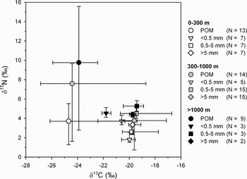
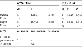
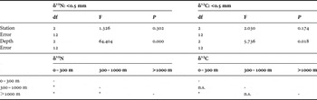
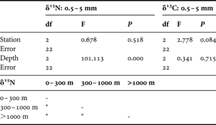
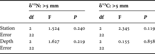
The distribution of δ15N and δ13C values of different zooplankton size-classes (<0.5 mm, 0.5–5 mm, >5 mm) and POM in the water column are represented as a plot of δ15N against δ13C values, grouped into three depth layers (0–300 m, 300–1000 m and >1000 m) (Figure 8). Values of all stations were pooled because no significant differences were detectable between the three sampling locations (ANOVA; Tables 10–13). δ15N and δ13C values of specific zooplankton taxa are also represented as a δ15N–δ13C plot (Figure 9).
δ15N–δ13C plot for different zooplankton size-classes and POM in different depth layers (night values). Error bars represent minimal and maximal values. N, number of samples; mean values of all stations.

δ15N–δ13C plot for specific zooplankton taxa (night values). Error bars represent minimal and maximal values. N, number of samples; mean values of all stations and depths.

One-way-ANOVA of δ15N and δ13C values of particulate organic matter (POM) for factors station (Rhodes Basin, Anaximenes saddle and summit) and depth, and matrix of pairwise comparisons after Bonferroni comparisons for δ15N differences between depth layers.
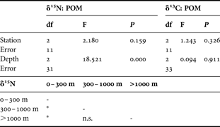
df, degrees of freedom; F, F ratio of mean squares; P, probability of correlation; *, P < 0.05; n.s., P > 0.05.
One-way-ANOVA of δ15N and δ13C values of zooplankton size-class <0.5 mm for factors station (Rhodes Basin, Anaximenes saddle and summit) and depth, and matrix of pairwise comparisons after Bonferroni comparisons of differences between depth layers.

df, degrees of freedom; F, F ratio of mean squares; P, probability of correlation; *, P < 0.05; n.s., P > 0.05.
One-way-ANOVA of δ15N and δ13C values of zooplankton size-class 0.5–5 mm for factors station (Rhodes Basin, Anaximenes saddle and summit) and depth, and matrix of pairwise comparisons after Bonferroni comparisons for δ15N differences between depth layers.
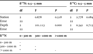
df, degrees of freedom; F, F ratio of mean squares; P, probability of correlation; *, P < 0.05; n.s., P > 0.05.
One-way-ANOVA of δ15N and δ13C values of zooplankton size-class >5 mm for factors station (Rhodes Basin, Anaximenes saddle and summit) and depth.
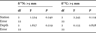
df, degrees of freedom; F, F ratio of mean squares; P, probability of correlation.
δ15N AND δ13C RATIOS OF ZOOPLANKTON SIZE-CLASSES AND POM
The plot of the stable isotope ratios shows an increase in δ15N values with depth for each zooplankton size-class and a trend of increasing δ15N with increasing organism size in each depth zone (Figure 8). In the upper 300 m highest δ15N values (2.3–4.1‰) were found in size-class >5 mm, while organisms <0.5 mm showed the lowest ones (1.5–2.5‰). In the mesopelagic zone (300–1000 m) highest δ15N values were measured for the size-class 0.5–5 mm (4.0–5.1‰); values for the other size-classes ranged from 3.3‰ to 4.3‰. Highest δ15N (4.7–5.8‰) in size-class 0.5–5 mm were also found below 1000 m, where values for zooplankton <0.5 mm and >5 mm ranged from 4.1‰ to 5.1‰. A one-way ANOVA confirmed the vertical trend with differences being significant between all depth layers (Tables 11–13).
The δ15N values of POM were generally higher than those of the zooplankton in each depth layer. A one-way ANOVA indicates significant differences between the pelagic zones for the stable nitrogen isotope ratios of POM (Table 10). The values varied strongly in each depth layer, ranging from 1.3‰ to 5.5‰ at 50 m and from 6.6–9.6‰ at 680/750 m. Below 1000 m values were concentrated in a range of 9.3–15.6‰ but there were also strongly differing values measured.
The δ13C ratios showed only small differences between the depths; only in size-class <0.5 mm the values decreased significantly from the epipelagic (−20.5‰ to −19.5‰) to the mesopelagic (−22.4‰ to −19.3‰) and the bathypelagic zones (−22.1‰ to −21.4‰). The isotope ratio of the fraction 0.5–5 mm showed a slight increase with increasing depth. In the upper 300 m values ranged between –20.5‰ and –19.7‰, between 300 and 1000 m values were measured from –20.7‰ to –16.7‰ and below 1000 m from –20.5‰ to –18.9‰. For organisms >5 mm no clear trend of the δ13C values could be observed. Values ranged from −20.6‰ to −17.1‰.
For POM δ13C ratios ranged from –26.1‰ to –20.3‰ in the upper 300 m and increased slightly below 300 m (–26.9‰ to –18.7‰). Generally, δ13C ratios were higher in zooplankton than in POM and showed a trend for slightly increasing values with increasing size of the organisms.
SPECIFIC ZOOPLANKTON TAXA
δ15N and δ13C ratios of specific taxa were measured for Pisces, Chaetognatha, Decapoda and the calanoid Copepoda Eucalanus spp., Haloptilus spp. and Lucicutia spp. The δ15N values of Pisces were concentrated in a range of 3.8–6.2‰ and those of Chaetognatha between 4.6‰ and 5.6‰ (Figure 9). For Decapoda δ15N values were measured between 3.0‰ in the upper 300 m and 5.2‰ below 1000 m. In case of Lucicutia spp. the δ15N values differed strongly between the epipelagic (1.6‰) and the bathypelagic zones in 2000–3500 m depth (10.8‰). The δ15N values of Haloptilus spp. in the upper 300 m ranged from 4.3‰ to 5.9‰, and Eucalanus spp. from the mesopelagic zone showed δ15N values between 5.4‰ and 6.8‰.
The δ13C values of Pisces ranged between –20.3‰ and –17.8‰ and the values of Chaetognatha between –19.8‰ and –19.6‰. For Decapoda δ13C values were measured in a range of –20.3‰ to –19.2‰. For Lucicutia spp. the surface value (–22.7‰) was lower than that measured in the bathypelagic zone (–20.2‰). The δ13C values of Haloptilus spp. ranged from –21.6‰ to –19.6‰ and that of Eucalanus spp. from –20.5‰ to –18.9‰.
DISCUSSION
The principal objective of this study was to investigate whether there is any difference in the vertical distribution and taxonomic composition of zooplankton and the trophic interactions in the northern Levantine Basin between the Anaximenes Mountain and the Rhodes Basin depending on current–topography interaction and surface circulation patterns.
Biomass, abundance and vertical distribution
Our results show both clear differences in zooplankton biomass and, by trend, slight differences in abundance between the Rhodes Basin and the Anaximenes Mountain region. But contrary to the common picture of enhanced zooplankton and micronekton biomass at seamounts as compared to the surrounding ocean (Genin & Boehlert, Reference Genin and Boehlert1985; Genin, Reference Genin2004), in our study zooplankton densities were lower at the seamount than at the reference location in the Rhodes Basin.
Enhanced zooplankton stocks at seamounts are often attributed to the retention effect of Taylor columns and elevated primary productivity through local upwelling. The undersea Anaximander Mountains are surrounded by the main jets in the Levantine Basin, namely the Asia Minor Current (AMC) and the Mid-Mediterranean Jet (MMJ). With a minimum depth of about 800 m the Anaximenes summit is located below the range of both jets. During the survey period the patterns of surface currents were analysed by weekly composites of dynamic topography and geostrophic currents from AVISO satellite altimetry from November 2006–January 2007 (Peine et al., Reference Peine, Turnewitsch, Mohn, Reichelt, Springer and Kaufmann2009). The results show that in the vicinity of the Anaximenes Mountain mesoscale variability was generally low in the sampling period, and enhanced levels of variability in Turkish coastal areas did not penetrate the seamount region. Below 400 m down to seamount summit depth (~750 m) ADCP recordings showed consistently low current velocities of approximately 3–4 cm s−1 and an oscillatory pattern in north-west–south-east directions dominating the flow variability (Peine et al., Reference Peine, Turnewitsch, Mohn, Reichelt, Springer and Kaufmann2009). Because of the low current velocities at the Anaximenes summit depth, the current–topography interaction might be not sufficient to create a Taylor column (see also Roden, Reference Roden1991; White & Mohn, Reference White and Mohn2005), which affects the advection and retention of particles and plankton above the summit.
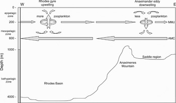
The sampling site in the Rhodes Basin was located within the sphere of the persistent Rhodes gyre. Within the Rhodes gyre, which is most intense and developed during the autumn–winter months from October until January (Malanotte-Rizzoli & Bergamasco, Reference Malanotte-Rizzoli and Bergamasco1989), a doming vertical structure is present, indicating an upwelling of relatively colder and less saline waters from deeper layers (Pancucci-Papadopoulou et al., Reference Pancucci-Papadopoulou, Siokou-Frangou, Theocharis and Georgopoulos1992; Theocharis et al., Reference Theocharis, Georgopoulos, Lascaratos and Nittis1993), enriching the surface waters with nutrients (Pancucci-Papadopoulou et al., Reference Pancucci-Papadopoulou, Siokou-Frangou, Theocharis and Georgopoulos1992; Mazzocchi et al., Reference Mazzocchi, Christou, Fragopoulu and Siokou-Frangou1997). Thus the permanent upwelling structure within the Rhodes gyre could be an explanation for the higher zooplankton biomass found during the present study at the sampling sites in the Rhodes Basin. The influence of the upwelling structure within the Rhodes gyre, increasing the zooplankton abundance in the surface layer at local stations, was also reported by Pancucci-Papadopoulou et al. (Reference Pancucci-Papadopoulou, Siokou-Frangou, Theocharis and Georgopoulos1992) and Mazzocchi et al. (Reference Mazzocchi, Christou, Fragopoulu and Siokou-Frangou1997). The same authors related lower zooplankton densities inside the Anaximander eddy to the influence of the anticyclonic downwelling within this feature. The following conceptual model presents the main currents and the possible correlations between the water mass circulation and the present zooplankton distribution in the study area. We assume that, dependent on the upwelling structure inside the Rhodes gyre, zooplankton density is enhanced in the surface waters of this region, while above the Anaximenes Mountain the lack of any local or larger scale upwelling structure or even the downwelling effect of the Anaximander anticyclonic eddy may result in a lower biomass and abundance in the upper water layers (Figure 10).
Conceptual model of water mass circulation in the Rhodes Basin and in the Anaximenes Mountain region. AMC, Asia Minor Current; MMJ = Mid-Mediterranean Jet (figure not to scale).

The vertical distribution patterns of biomass and abundance were very similar in all three areas, with the smallest size-class (<0.5 mm) decreasing strongly from the surface to depth, whereas larger zooplankton shows a less clear pattern with high variability in the upper 1500 m. Usually the maximum concentration of mesoplankton is confined to the upper 100 m layer before it sharply and often unevenly decreases down to the lower layers of the mesopelagic zone, as pointed out by Vinogradov & Tseitlin (Reference Vinogradov, Tseitlin and Rowe1983). Depending on the hydrologic regime and the seasonal cycles of the communities, layers with sharply decreasing biomass alternate with layers where biomass decreases considerably less. The change from surface to mid-water plankton between 200 and 300 m and the change from mid-water to bathypelagic plankton below 1500 m were obvious in the present study. This feature was marked by the vertical distribution of the main copepods (0.5–2 mm) of the genera Haloptilus in the epipelagic zone, Eucalanus in the mesopelagic zone and Lucicutia in the bathypelagic zone. The total quantity of plankton in the meso- and bathypelagic zone is directly dependent on the quantity of epipelagic mesoplankton (Vinogradov & Tseitlin, Reference Vinogradov, Tseitlin and Rowe1983), featuring the assumption that zooplankton <0.5 mm is continuously fed by larger organisms below 200 m. Another explanation for the strong decrease of the smallest size-class (<0.5 mm) throughout the water column might be the lack of vertical migration in this size-group, whereas larger interzonal species performing diurnal migrations from the surface to 400–800 m, feature a more heterogeneous distribution pattern. An increasing biomass proportion of larger zooplankton (>2 cm) to the total net plankton biomass with increasing depth, as found during the present study, is also known for oligotrophic tropical regions of the Pacific and the Indian Oceans and for the north-west Pacific (Vinogradov & Tseitlin, Reference Vinogradov, Tseitlin and Rowe1983) as well as for Sedlo, Seine and Ampère Seamounts in the north-east Atlantic (Martin & Christiansen, Reference Martin and Christiansen2009).
Composition
Based on previous observations at Seine and Sedlo Seamounts (Martin & Christiansen, Reference Martin and Christiansen2009; Martin & Christiansen, unpublished) and Great Meteor Seamount (Martin & Nellen, Reference Martin and Nellen2004) in the north-east Atlantic we expected the zooplankton above the Anaximenes summit to be mainly composed of smaller taxa like cyclopoid copepods and small members of Calanidae, and the occurrence of larger organisms (>5 mm) to be reduced or even lack, in comparison to the Anaximenes saddle region and the reference station. However, the taxonomic composition above the Anaximenes did not differ markedly from the saddle region or the reference station in the Rhodes Basin and the expected spatial pattern of size distribution was not found. But we cannot exclude that possible differences between the areas were not detected due to the mesh selection of the nets used, which sampled quantitatively only macrozooplankton and larger mesozooplankton.
Copepod carcasses have often been found to be more abundant above the summit plateau of seamounts than in deeper waters surrounding the slope (Haury et al., Reference Haury, Fey, Gal, Hobday and Genin1995, Reference Haury, Fey, Newland and Genin2000; Martin & Nellen, Reference Martin and Nellen2004; Martin & Christiansen, unpublished). However, above the deep Anaximenes summit accumulations of exoskeletons could not be detected. Genin et al. (Reference Genin, Haury and Greenblatt1988, Reference Genin, Greene, Haury, Wiebe, Gal, Kaartvedt, Meir, Fey and Dawson1994) and Haury et al. (Reference Haury, Fey, Newland and Genin2000) supposed that high numbers of exoskeletons above the plateau result from enhanced predation at summit depth by seamount residents, caused by accumulation of vertically migrating zooplankton above the bottom, and from the possible accumulation of sinking carcasses at these depths. Our findings show that there was no enhanced predation caused by a higher food supply above the Anaximenes summit, probably because interactions of vertically migrating zooplankton with the bottom residents in ~800 m depth were negligible, and the low retention potential due to the lack of Taylor column-like structures did not allow for the accumulation of exoskeletons.
Food web structure
No significant differences in the food web structure were detectable between seamount and reference station, and the δ15N and δ13C signatures gave no indication of differing food availability at the sampling locations. In the following, the trophic structure, based on stable isotope ratios, will be summarized for all sampling locations.
Zooplankton stable nitrogen isotope ratios in the surface waters were generally low, as compared to, e.g. zooplankton of the Atlantic Shelf of the Iberian Peninsula (Bode et al., Reference Bode, Alvarez-Ossorio, Cunha, Garrido, Peleteiro, Porteiro, Valdes and Varela2007), but similar to the values found by Koppelmann et al. (Reference Koppelmann, Weikert and Lahajnar2003, Reference Koppelmann, Böttger-Schnack, Möbius and Weikert2009) in the Ierapetra Deep in April 1999 and also in the Levantine Basin in October 2001. In the Atlantic, nitrate is the main nitrogen source for primary production, whereas in the eastern Mediterranean atmospheric nitrogen may play an important role for primary production through nitrogen fixing cyanobacteria, resulting in the low δ15N values in this regime, as supposed by several authors (Sachs & Repeta, Reference Sachs and Repeta1999; Pantoja et al., Reference Pantoja, Repeta, Sachs and Sigman2002; Koppelmann et al., Reference Koppelmann, Weikert and Lahajnar2003, Reference Koppelmann, Böttger-Schnack, Möbius and Weikert2009). Assuming a mean δ15N increase of 3.4–3.6‰ per trophic level (Minagawa & Wada, Reference Minagawa and Wada1984; Hobson & Welch, Reference Hobson and Welch1992; Post, Reference Post2002), the δ15N values of zooplankton in the surface waters of the northern Levantine Basin indicate that their main food source, such as phytoplankton, organic particles and smaller zooplankton, has δ15N values around zero, which is in the range of δ15N signatures of nitrogen fixing organisms (–2‰–1‰; Mullin et al., Reference Mullin, Rau and Eppley1984; Minagawa & Wada, Reference Minagawa and Wada1986; Carpenter et al., Reference Carpenter, Capone, Fry and Harvey1997). Consequently, it is supposed that the whole eastern Mediterranean system is based on a nitrogen source with low δ15N values.
In the present study we expected an increase of δ15N and δ13C along the food chain as well as an enrichment of 15N and 13C in zooplankton and POM with increasing depth. Differences in the δ15N and δ13C signatures between zooplankton size-classes were smaller in meso- and bathypelagic depths than in the upper layers, indicating restricted food availability below the photic zone. The most likely food source of mesozooplankton is phytoplankton and sinking and suspended POM. But our results gave no clear information about how POM as food source is used by different zooplankton size fractions. The differences in δ13C between POM and zooplankton were generally higher than the usual enrichment of 0.4–1‰ from one trophic level to the next higher (DeNiro & Epstein, Reference DeNiro and Epstein1978; Michener & Schell, Reference Michener, Schell, Lajtha and Michener1994; Post, Reference Post2002), indicating a different and unknown food source. Contrary to our expectations, higher δ15N values were found in suspended POM than in zooplankton organisms in the surface layers, while in meso-and bathypelagic depths values of both were similar. Koppelmann et al. (Reference Koppelmann, Böttger-Schnack, Möbius and Weikert2009) found lower δ15N values in suspended POM in the surface waters south-east of Crete than we did in the northern Levantine Basin in comparable depths, whereas the values in meso- and bathypelagic depths were concentrated in a similar range at both study sites. Perhaps the higher surface values in the northern Levantine Basin indicate the uplift of mid-water layers in the cyclonic Rhodes gyre, as low mid-water suspension values reflect the deepening of the upper layer in the anticyclonic Ierapetra gyre (Koppelmann et al., Reference Koppelmann, Böttger-Schnack, Möbius and Weikert2009).
The dominating zooplankton genus in the subsurface zone between 100 and 300 m was the calanoid copepod Haloptilus. Its δ15N signature was even higher than in Chaetognatha, as reported by Koppelmann et al. (Reference Koppelmann, Böttger-Schnack, Möbius and Weikert2009) for the Ierapetra Deep as well, and reflects the carnivorous feeding of this organism (Timonin, Reference Timonin1971; Beckmann, Reference Beckmann1995).
From 300 to 1000 m the zooplankton community was dominated by Eucalanus spp. Eucalanus species are known as herbivorous coarse-filter feeders (Timonin, Reference Timonin1971; Beckmann, Reference Beckmann1995), and their δ15N signature corresponded largely to the δ15N values of POM. But in terms of the δ13C signatures the difference between POM and Eucalanus spp. was much higher than the usual enrichment between trophic levels (DeNiro & Epstein, Reference DeNiro and Epstein1978; Michener & Schell, Reference Michener, Schell, Lajtha and Michener1994; Post, Reference Post2002). One explanation might be that earlier life stages of these interzonal migrators used other food sources than CV stages, which are remaining for diapause in meso- and bathypelagic depths during winter (Smith, Reference Smith1995).
The observed increase of δ15N and the trend of 13C enrichment in zooplankton organisms with increasing depth indicate a longer food chain in mid and deep-sea waters than in surface layers. Throughout the water column an enrichment of the heavier 15N and 13C isotopes in sinking POM is caused by microbial degradation and faecal pellet production, resulting in enhanced δ15N and δ13C values in detrivorous and omnivorous zooplankton, which use sinking and suspended organic material as main food source. This is evident, e.g. in species of the omnivorous copepod Lucicutia: epipelagic Lucicutia species had very low δ15N values, whereas bathypelagic Lucicutia spp. showed a high δ15N ratio, corresponding to δ15N values in POM at this depth. Similar differences have been reported by Koppelmann et al. (Reference Koppelmann, Böttger-Schnack, Möbius and Weikert2009) for the Ierapetra Deep in October 2001, and it is supposed that Lucicutia spp. probably feed on suspended particles as well as on remains of decomposed bodies and bacteria. Corresponding to the δ15N signatures, epipelagic Lucicutia species had lower δ13C values than bathypelagic species, and surface POM showed a lower 13C content than deep-sea POM. Studies in the western Mediterranean by Polunin et al. (Reference Polunin, Morales-Nin, Pawsey, Cartes, Pinnegar and Moranta2001) showed a similar tendency of higher δ13C ratios in zooplankton at greater depth, consistent with the degradation of POM leaving residual material of inorganic carbonates and chitin, which are enriched in 13C compared to other biochemical fractions (Bunn et al., Reference Bunn, Loneragan and Kempster1995). However, information about trophic interactions between organic material, bacteria and zooplankton is still scarce for the deep Levantine Basin.
The carnivorous Chaetognatha and Pisces studied had relatively low δ15N values, pointing to a trophic position about one level higher than mixed zooplankton <0.5 mm, but lower than the larger size zooplankton classes. This indicated that they fed mainly on cyclopoid Copepoda and small Calanidae, which was supported by the corresponding difference in δ13C. Pisces were mainly composed of Cyclothone spp. and species of the family Myctophidae, known for their planktivorous diet (Whitehead et al., Reference Whitehead, Bauchot, Hureau, Nielsen and Tortonese1984). In case of some planktivorous fish species diel vertical migration and associated feeding at the surface could be a reason for the relatively low δ15N values as well, although the most abundant fish in our study, Cyclothone is known as non-migrating (Whitehead et al., Reference Whitehead, Bauchot, Hureau, Nielsen and Tortonese1984). Compared with omnivorous and detrivorous zooplankton, nitrogen and carbon stable isotope ratios of planktivorous taxa changed only slightly throughout the water column.
CONCLUSIONS
The zooplankton community in the Anaximenes Mountain region in the northern Levantine Basin seemed not to be influenced by a seamount effect. Possible reasons may be the topography of this seamount combined with the hydrographic conditions. The Anaximenes Mountain forms an elongated elevation without a wide summit plateau, and current velocities at summit depth were low during the study. Because of only little interaction between the complex topography and the main currents AMC and MMJ, a Taylor column above the Anaximenes Mountain can probably not develop. Instead of these local effects larger scale processes like the cyclonic Rhodes gyre seem to dominate the area, and may drive the difference in zooplankton distribution between the seamount and the Rhodes Basin. However, no significant differences between both locations were evident in the food web. Stable isotope signatures showed, at a generally low level, enrichment in zooplankton taxa along the food chain within the different pelagic zones and from the surface to the deep-sea. But it has to be considered that only three trophic levels of the food chain without top predators were studied. The primary food source of the zooplankton community in the study areas remains unclear. Although the very low δ15N values of POM at the surface, which stress the importance of nitrogen fixing primary producers, support the assumption that herbivorous zooplankton feeds on POM, the δ13C signatures point to a different food source at an intermediary step between both compartments.
ACKNOWLEDGEMENTS
Our thanks go to the crew of RV ‘Meteor’ and our colleagues on board for their help and assistance with sampling and for making the cruise successful. U. Struck kindly analysed the stable isotopes of the zooplankton samples. The study was funded by grants of the Deutsche Forschungsgemeinschaft (DFG CH 172/5-1).