III. RESULTS AND DISCUSSION

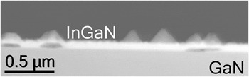
The investigated sample is one from a series of In _x Ga_1−x N thin films of different indium content. The initially flat film surfaces have been shown to roughen with increasing value of x, leading to islands with pronounced facets for x > 0.5. At the same time, dark field imaging has shown a corresponding increase in speckle contrast from the alloys. ^{Reference Wang, Chauvat, Ruterana and Walther18} This is exactly the compositional range for which phase separation has previously been identified as likely from x-ray diffraction. ^{Reference Bartel, Specht, Ho and Kisielowski21} While such high indium content is not typical for present InGaN quantum wells used for commercial LEDs, it may become relevant in the future if lower bandgaps will be approached to circumvent the use of yellow phosphors in combination with blue LEDs to produce green, or orange, light emission more directly. ^{Reference Orsal, El Gmili, Fressengeas, Streque, Djerboub, Moudakir, Sundaram, Ougazzaden and Salvestrini22} Moreover, carrier confinement in thin quantum wells and small quantum dots can complicate the interpretation of emission and bandgap properties, so our thin film sample can serve as an easier to understand model system. A typical overview image of our sample with x _nom = 0.62 is depicted in Fig. 1 where several facetted islands can be clearly seen. Some of these seem to preferentially nucleate above apparent holes in the underlying film; however, these holes are partially filled by carbonaceous species and it is not yet clear whether they are an artifact from preferential argon ion thinning and subsequent filling by sputtered glue. We have used integral measurements by energy-dispersive x-ray spectroscopy (EDXS) at 197 kV to verify the average In content of each sample, using a recently improved quantification method based on thickness-dependent, self-consistent k-factors ^{Reference Walther23,Reference Walther and Wang24} which eliminates discrepancies between absorption corrections for areas of different thicknesses ^{Reference Amari, Ross, Wang and Walther25} and has given excellent linearity with the observed shift of the plasmon peak energy in EELS. ^{Reference Wang, Chauvat, Ruterana and Walther18} None of the regions investigated at higher magnifications in subsequent figures can be marked in the overview of Fig. 1 because, being much thinner, they are outside its field of view, as we tried to avoid irradiating these regions at 200 kV prior to chemical analysis at 60–100 kV, which could have implied beam electron beam damage as explained above.

FIG. 1.

ADF STEM image of cross-sectioned In_0.62Ga_0.38N thin film at low magnification. JEOL 2010F, 197 kV, 9.5 mrad convergence semi-angle, 55–170 mrad collection angle, 2.5 μm field of view.

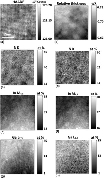
In Fig. 2 we show results from an investigation of a very small area at high magnification by mapping high-energy core losses in EELS at 100 kV without monochromation.

FIG. 2.

(a) HA-ADF-STEM image of cross-sectioned In_0.62Ga_0.38N film at high magnification, about 10 nm above the GaN substrate, showing (0002) lattice fringes. Growth direction points upwards. (b) Relative thickness map (t/λ) in multiples of the inelastic mean free path, λ. (c–h) Results from spectrum imaging: elemental maps of (c, d) nitrogen from N K edge, (e, f) indium from In M_4,5 edge, (g, h) gallium from Ga L_2,3 edge, recorded at 100 kV and calculated using (c, e) integration after inverse power law subtraction, (g) integration after exponential background extrapolation or (d, f, g) from model based multiple linear-least squares fitting of the edge intensities, all normalized to a sum of unity for all three elements. NION UltraSTEM, 100 kV, 30 mrad convergence semi-angle, 90 mrad inner collection angle (HA-ADF), 45 mrad collection angle (EELS), 50 ms dwell time per pixel, 128 × 128 pixel, 0.5 eV/channel, 7 nm field of view.

Figure 2(a) displays a high-angle annular dark-field (HA-ADF) image of a section ∼7 nm wide near the bottom of the InGaN thin film, close to a $\left\langle {{1 {\bar100}}} \right\rangle$ zone axis orientation. The growth direction points upwards, and clear (0002) lattice fringes (d ₀₀₀₂ = 0.26 nm) running along the horizontal and in some areas weak $\left( {{{11\bar 20}}} \right)$ lattice fringes $\left( {{d_{11\bar 20}} = 0.16\,{\rm{nm}}} \right)$ along the vertical are visible. The apparent waviness of the lattice planes is due to slight thermal drift using the acquisition. We did not use any drift correction as this would have necessitated additional reference image collection and thus would have slowed down acquisition and increased the total dose. All images and maps shown were acquired rotated through almost 90°, and the fine vertical stripes visible in parts of Fig. 2(a) are due to emission fluctuations typical of the cold field emitter. Figure 2(b) is a relative thickness map of the area calculated from the intensity ratio of the zero loss peak to the total intensity, and when we use a value of λ = 55 ± 9 nm for the inelastic mean free path extrapolated from tabulated semiconductor values recorded at 100 kV for different acquisition angles (Table 5.2 on page 304 of Ref. Reference Egerton26) the value of t/λ = 0.69 ± 0.03 measured for this sample region would indicate the specimen area investigated here is slightly less than 40 nm thin. The above inelastic mean free path is smaller than typical values for most semiconductors at 100 or 200 kV because of the large entrance aperture used (45 mrad reduces λ to 3/4 of the value for 10 mrad listed in Ref. Reference Egerton26), and the heavy indium atoms in In_0.6G_0.4N reduce it even further. 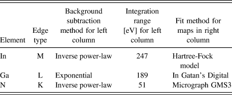Figures 2(c)–2(h) are elemental maps of the distribution of the three elements nitrogen, indium, and gallium calculated using two different methods for fitting the data, using either a pixel-wise automated edge detection routine ^{Reference Angadi, Abhayaratne and Walther27} with inverse power-law or exponential background fit and subtraction in the pre-edge regions, net integration over certain ranges and quantification using tabulated Hartree-Slater cross-sections or a recursive multiple linear-least squares fitting to Hartree-Slater models of edges tabulated in Gatan Digital Micrograph GMS3 Software. ^{Reference Thomas and Twesten28} Details are reported in Table I. The speckle contrast in these maps is a superposition of shot noise (which should depend only on the acquired data and therefore be the same in left and right columns) but also to some degree due to the different background subtraction and fit procedures (where the two algorithms used differ). The relative quantification has been normalised to a sum of unity taking into account only these three elements. There was a very faint oxygen signal from the surface which has been neglected. Both methods agree, within noise levels, for the quantification of the gallium content from the Ga L edge (g: 15.2 ± 5.9 at.%, h: 14.6 ± 4.5 at.%), which would imply an average x value for In _x Ga_1−x N of x = 0.7 ± 0.1. The Ga L-edge starts at very high energy (1115 eV) so its intensity is weak and the maps will be mainly limited by shot noise, while background subtraction is relative straight forward and implies small systematic errors. For the quantification of the N K-edge and the In M-edge the situation is reversed: these edges lie at lower energies and so have plenty of intensity but they partially overlap (the N K-edge starts at 400 eV, the In M-edge at 443 eV) so they are more difficult to separate. Correspondingly, the indium maps in (e) and (f) show the same features but on different contrast levels (e: 48.9 ± 5.4 at.% indium; f: 25.5 ± 4.2 at.% indium). The quantification with the higher apparent indium signal predicts less nitrogen, and vice versa. The nitrogen content as calculated from the N K-edge by the two algorithms lies either below the stoichiometric 50 at.% value (c: 35.9 ± 1.5 at.%) or above (d: 60.9 ± 2.1 at.%), indicating systematic errors of about the same magnitude but in opposite directions where our algorithm ^{Reference Angadi, Abhayaratne and Walther27} systematically underestimates the N content by about as much as the commercial algorithm ^{Reference Thomas and Twesten28} overestimates it. Deconvolution of the spectra could change the relative quantification further but has not yet been attempted here, as it would have been difficult to record low- and high-loss spectra without the dual-EELS option ^{Reference Scott, Thomas, MacKenzie, McFadzean, Wilbrink, Craven and Nicholson29} and we could use integration ranges sufficiently wide for the N and Ga edges to include plasmon replicas so (multiple) plasmon scattering would cancel out in the ratio approach taken. However, it should be stated that the relative quantification of InGaN is a real challenge, firstly, as it implies evaluating three ionization edges of different types (K, L, and M) and, secondly, because two edges of these overlap significantly. The standard deviations of the N maps in (c) and (d) are very small, as would be expected for a constant group-V sub-lattice consisting of N only. The maps for In and Ga show much larger scatter, with 2–3 times higher standard deviations. The lateral scale of the indium-rich regions visible in (e) and (f) extends to only 0.5–3 nm, which would be in agreement with Jinschek et al. ^{Reference Jinschek, Erni, Gardner, Kim and Kisielowski30} Given the projection through the ∼40 nm thick specimen such In-rich clusters, should they exist and not be an artifact from electron irradiation, must consist of almost pure InN. Extremely short-range fluctuations of the chemical composition (on a lateral scale <1 nm) have been speculated about previously while medium range order on the scale >2 nm was shown to not influence the optical properties of InGaN quantum wells, ^{Reference Albrecht, Grillo, Borysiuk, Remmele, Strunk, Walther, Mader, Prystawko, Leszczynski, Grzegory and Porowski31} which agrees with our findings shown later in Fig. 10.

TABLE I.

Processing details for elemental maps displayed in Fig. 2.

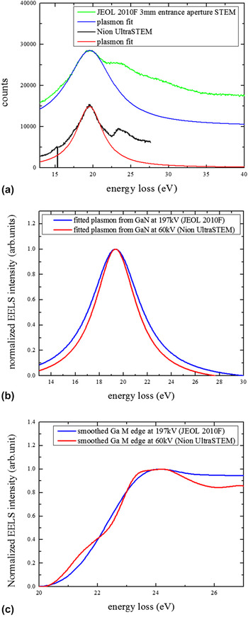
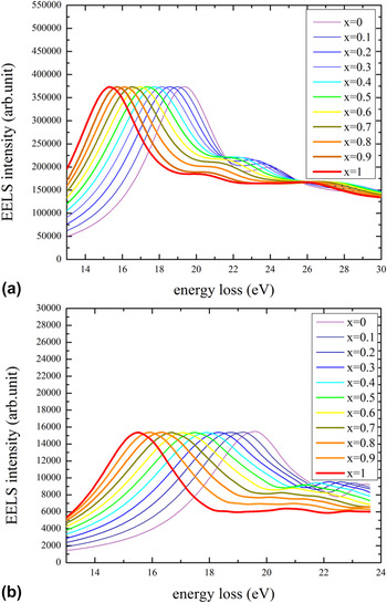
To suppress the beam damage issue already mentioned we have also performed EELS at a reduced acceleration voltage of 60 kV where potential knock-on damage should be completely negligible, even at higher dose. A comparison of monochromatic EELS at 60 kV in the Nion UltraSTEM with cold field-emitter to EELS at 197 kV in a standard JEOL 2010F with Schottky-field emitter has been performed for pure GaN. Figure 3 shows (a) raw spectra with Lorentz fits of the plasmons for both microscopes (from 13 to 40 eV for the 197 keV spectrum and 13–27 eV for the 60 kV spectrum), and best fits for (b) the plasmon loss component and (c) the Ga M core loss component only where the latter was extracted as the remainder after fitting the plasmon peak by a Lorentz function as shown and then subtracting it off from a smoothed version of the low-loss spectrum. The zero loss peak was subtracted prior to the fits and thus not included. The differences are subtle, with a slightly reduced plasmon peak width and a slight undulation of the Ga core loss signal at the lower acceleration voltage which we tentatively attribute to the individual onsets of M₅, M₄, and M₃ partial edges that become visible when the acceleration voltage is reduced, the energy resolution improved and the collection angle increased. In other words, the plasmon has not really become narrower at lower acceleration voltage but the fitting routine transferred some of the broadening of the core losses at 197 kV due to the higher aberrations of the older spectrometer to the plasmon loss region. This directly meant that the database of InGaN reference spectra previously acquired for 197 kV in the JEOL microscope [see Fig. 4(a)] had to be compiled afresh, now for monochromated measurements at 60 kV. Our approach was to extract high quality spectra from the GaN buffer region and the InGaN layer, and to subtract the Ga core losses from Fig. 3(c) from the latter to obtain references for pure InN, then interpolating InGaN data in a way analogous to the one described in Ref. Reference Wang, Chauvat, Ruterana and Walther17. This resulted in the new set of compiled InGaN reference spectra shown in Fig. 4(b).

FIG. 3.

Comparison of (a) low-loss EELS from GaN recorded at 197 kV in the JEOL 2010F (green, with blue fit to plasmon) and at 60 kV in the NION UltraSTEM (black, with red fit to plasmon). Comparison of fits for (b) plasmon loss and (c) Ga M-edge core loss components.

FIG. 4.

Comparison of GaN reference spectra for x = 0 to x = 1 at (a) 197 kV ^{Reference Wang, Chauvat, Ruterana and Walther17} and (b) 60 kV. Note the different scale chosen to correlate with the experimental dispersions of (a) 0.05 eV/channel (1024 channels) and (b) 0.015 eV/channel (2048 channels).

Figure 4 compares reference EELS spectra for InGaN alloys of different indium content, x, generated from experimental spectra recorded for GaN, InN and some InGaN alloy thin films whose average x values were previously determined by EDXS. These spectra are used as database for multiple linear least-squares fitting. In this work, we used the data shown in Fig. 4(b) for monochromated EELS at 60 kV.

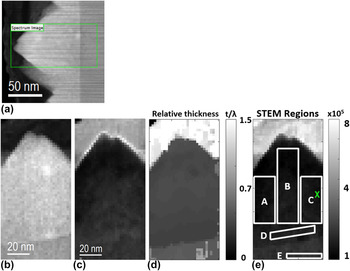
A region of the InGaN layer with a facetted island of almost uniform thickness in projection, as shown in Fig. 5, has been used for further investigation by EELS of the low-loss region up to 24 eV. The speckle contrast in Fig. 5(b) stems from a superposition of carbon contamination and chemical inhomogeneities in this region both of which are unlikely to be due to beam damage as they are already visible in the fast scan acquired prior to the spectrum imaging, as shown in Fig. 5(a). Extrapolating the inelastic mean free path of 55 nm at 100 kV to 61 nm at 60 kV, the above value of t/λ = 0.43 ± 0.02 would imply an absolute specimen thickness around 26 nm, with an error of ±4 nm, but constant over the field of view to within ±1 nm. This shows the area investigated in detail in the following is suitably thin and flat.

FIG. 5.

(a) ADF overview image of InGaN islands, grown from right to left, with scan lines visible due to fast acquisition (32 μs dwell time per pixel, 500 × 500 pixel, as acquired), (b) rotated ADF image of the area investigated with 2.1 nm sampling where the apparent slight tilt from vertical growth is due to drift during the acquisition of (c) the spectrum image (0.5 s dwell time per pixel, 30 × 60 pixel, 0.015 eV/channel). (d) Relative thickness map for spectrum imaging at 60 kV, with mean values of t/λ = 1.52 ± 0.14 in the top carbon region, 0.43 ± 0.02 in the InGaN layer (which is, hence, almost uniformly thin) and 0.59 ± 0.13 in the GaN buffer. (e) Definition of regions A–D in the InGaN and region E in the GaN buffer used later in Table II. The cross marks the position of the spectrum and its fit shown in Fig. 6(i). Nion UltraSTEM, 30 mrad convergence, 90 mrad inner collection angle for HA-ADF, 45 mrad collection angle for EELS.

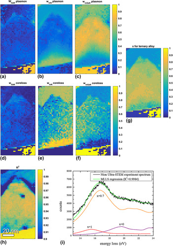
Fitting each spectrum within the 2D spectrum image has been performed on a linear least-squares method, decomposing each spectrum into a GaN, an InN and a ternary In _x Ga_1−x N component where the four fitting parameters are the three relative weight components, w _GaN, w _InN, w _InGaN and the indium component x _alloy for the ternary alloy component only. These fit parameters are plotted in Figs. 6(a)–6(g) for plasmon and core losses. Figure 6(h) shows a plot of the R ² parameter of the fit, indicating good fit quality, with R ² > 0.9 in all cases and R ² > 0.98 in most regions. Two spots within the InGaN with pronounced lower R ² values probably indicate carbon contamination spots rather than the onset of beam damage, as they are not visible in any of the maps in Figs. 6(a)–6(g). All weight parameters lie between 0 and 1 without applying any further constraints and are hence physically meaningful. The weights from plasmon and core loss fitting agree extremely well, indicating the lower part of the InGaN is almost pure InN (with some GaN and little In_0.5Ga_0.5N) while the upper part of the island is mostly ternary In _x Ga_1−x N with x decreasing from x ∼0.8 to ∼0.5 near the surface. The GaN is either fitted as binary GaN (near the bottom right of the maps) or ternary In_0.05Ga_0.95N (near the bottom left), and this is presumably due to the selection of Δx = 0.05 increments for the fitting of the ternary alloy composition (checking for all possible discrete values of the ternary allow component would have slowed down the pointwise fitting procedure enormously).

FIG. 6.

Results from fitting each spectrum from the spectrum image in Fig. 5(b) by a linear superposition of three reference spectra, one for GaN, one for InGaN and one for InN film. Shown are the weight parameters attributed to (a, d) GaN, (b, e) InN and (c, f) In _x Ga_1−x N where x was varied from 0.05 to 0.95 in steps of 0.05. Top row: fit for plasmons, middle row: fit for core losses. (g) plots the best fitting x value of the ternary component only. (h) shows the R ² parameter of the fit for each spectral data point. (i) shows the fit (green) for the experimental EELS (black) at one particular pixel marked in region C of Fig. 5(e) based on a weighted superposition of reference spectra from GaN (red), InN (purple) and In_0.7Ga_0.3N (orange).

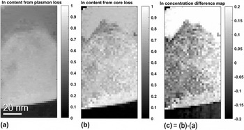
Figure 7 compares quantitative maps of the indium content, x, obtained from the relative weights of the plasmon and the low core-loss fits from the previous figure, where x = w _InN + x _alloy w _InGaN. Generally, the map from the core losses (7b) has somewhat higher contrast but also higher noise levels. The map from the plasmons (7a) appears smoother but lower in overall contrast, and in the GaN the x value predicted lies significantly above zero level. Both methods indicate indium enrichment within the first 15 nm of InGaN grown on the GaN buffer, where the core loss fitting would indicate almost pure InN (x ∼0.9) whereas the plasmon loss fitting would suggest a maximum of around x ∼0.8. Given the precision of the individual fits, increments of ∆x = 0.05 were tested for the ternary component, error bars of this order may well be expected and the difference between Figs. 7(a) and 7(b) is typically within this range for most of the InGaN.

FIG. 7.

Maps of indium content, x, calculated for data from Fig. 6 from weights of fitting (a) plasmon losses, (b) low core-losses, (c) difference map (b)–(a).

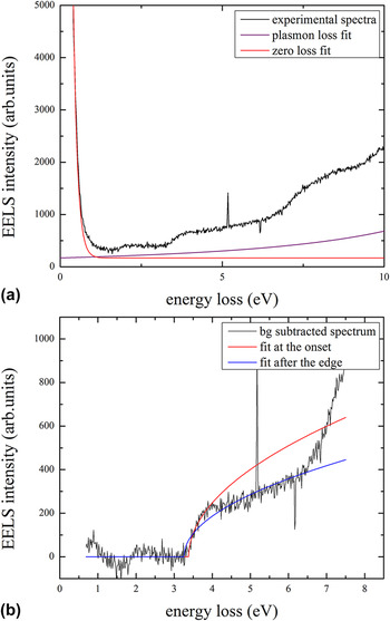
A monochromator with a slit in the energy-dispersive plane not only has the advantage of narrowing down the zero-loss peak but it also eliminates asymmetries due to the tails of the Fowler–Nordheim distribution for field emission and the Maxwell–Boltzmann distribution for heated filaments, ^{Reference Erni and Browning32} and the intensity retained is proportional to the slit width and hence easily predictable. ^{Reference Walther and Stegmann33} When we attempt to fit the VEELS, the net intensity after background subtraction does not follow an ideal behavior ∝√(E − E _g), as would be expected from the density of states (DOS) for a bulk semiconductor with direct bandgap, E _g. The observed intensity increases steeper initially (close to linearly), then flattens before it again rises drastically. Fitting a square-root function near the DOS onset [red line in Fig. 8(b); fit window 3.35–3.98 eV] gives a maximal R ² = 0.8933 and E _g = 3.38 eV, which is a reasonable value for GaN. Fitting after the DOS onset [blue line in Fig. 8(b), fit window 2.85–6.41 eV] only gives R ² = 0.7861 and a lower apparent value of E _g = 3.26 eV. This shows some of the problems encountered when attempting to fit a square-root type DOS to high-quality EELS data: good fits do not necessarily produce the correct edge-onset, and if the fit windows are moved (or even constant offsets taken into account to model ZLP tails and/or a background possibly due to Cherenkov radiation) then the number of fitting parameters becomes large and several combinations can fit a spectrum reasonably well, however, which edge onset is most reliable is difficult to judge. This is a fundamental issue for determining bandgaps from VEELS, and for GaN, explored more fully in Fig. 9, the random-mean-square (rms) uncertainty in absolute bandgap determination remains of the order of ±0.1 eV even for a monochromated instrument with an energy resolution far better than this (while fitting an analytical function over several channels could in theory produce sub-channel accuracy).

FIG. 8.

Valence EELS of GaN from region E with (a) extrapolations of zero loss and plasmon loss peaks, (b) square-root fits to onset of spectrum intensity after zero loss and plasmon loss subtraction.

FIG. 9.

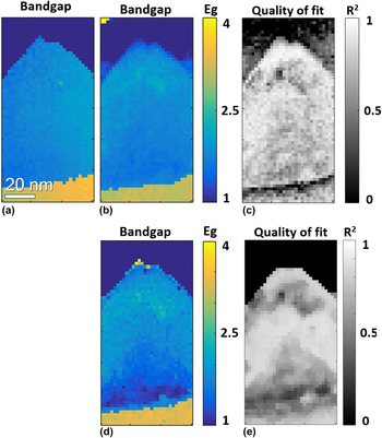
Maps of (a, b, d) extracted direct bandgap E _g (in eV) and (c, e) R ² for fits in (b, d), respectively, calculated for each point of spectrum image shown in Fig. 5. (a) has been calculated by extracting the VEELS from 0.7 eV to 4 eV, smoothing it, fitting a spline function, differentiating it and finding the maximum in the first derivate map. This is quick and easy to process but provides no R ² values as it is not a fit procedure. (b) has been calculated by subtracting a constant offset to account for zero loss and plasmon loss tails before fitting a function of form 300×√(E − E _g) over a 1 eV window in the range from 0.7 to 5 eV and maximizing R ². (d) has been calculated by modeling and subtracting exponential tails for the ZLP and Lorentzian tails for the plasmon; the rest has been done as for (b).

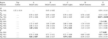
The low-loss region directly after the zero loss peak (but overlapping with its tails) is due to interband transitions and thus reflects the density of states (DOS) near the conduction band. A simple differentiation after smoothing [Fig. 9(a)] or calculation of the net signal by subtracting a constant offset to account for zero loss and plasmon loss tails [Fig. 9(b)], a rather common procedure, before fitting a square-root function of form 300×√(E − E _g) over a 1 eV window in the range from 0.7 to 5 eV and maximizing the R ², yield qualitatively similar maps. Method (b) seems to work well in most areas except in the direct vicinity of the InGaN/GaN interface where the corresponding R ² map in (c) decreases sharply. (d) has been calculated by subtracting exponential tails for the ZLP and Lorentzian tails for the plasmon; the rest has been done as for (b). This yields a slightly better curve fitting over-all and in particular near the InGaN/GaN interface region, but it yields comparably poor fits in the lower part of the InGaN. A complete numerical evaluation is included in Table II, demonstrating that even with superb energy resolution bandgap determination from VEELS is not as unambiguous as sometimes thought, and a precision better than the energy resolution of the spectrometer is probably not achievable due to ambiguities in removing zero loss peak and plasmon peaks. Our observation seems to be in good agreement with previous attempts of GaN bandgap measurements by VEELS, all of which reported error bars in the 0.1–0.2 eV range ^{Reference Brockt and Lakner34–Reference Manual, Koch, Özdöl, Sigle, van Aken, Garcia and Morales36} and, together with the additional problem of Cherenkov losses in most semiconductors, ^{Reference Stöger-Pollach and Schattschneider37} might explain why VEELS seems to generally work well for wide-bandgap materials ^{Reference Müllejans and French38} or semiconductors where the bandgap is known a priori but can fail to correctly predict the bandgap of unknown semiconductor structures. ^{Reference Specht, Ho, Xu, Armitage, Weber, Erni and Kisielowski39,Reference Erni and Browning40}

TABLE II.

Numerical results for regions of the maps and spectra analyzed. Values in italics are considered unreliable (low R ²) while those in bold are considered more reliable (high R ²).

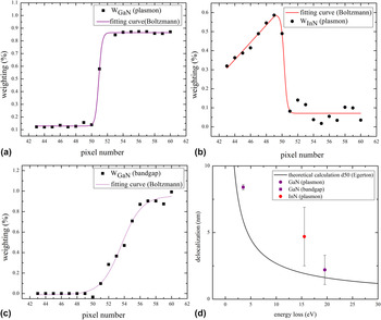
It can be clearly seen from Fig. 10 that the plasmon transitions across the InGaN/GaN interface (the top row in the figure) are much sharper than the change in bandgap in Fig. 10(c) (bottom left), from the same spectrum image data, and the delocalization observed is in reasonable agreement with that expected from a simple model that evaluates the spatial resolution as the diameter d ₅₀ that contains 50% of the intensity from a Fourier transform of the finite energy and thus also finite momentum transfer based on mean scattering angles and finite collection aperture. This directly demonstrates plasmon losses may be regarded as local within the sampling limit of a few nanometres (here: 1–2 pixels, i.e., 2–4 nm), while the bandgap is delocalized on a much wider scale. Physically, there would be no point in the definition of the bandgap for a crystal region smaller than that needed to hold a sufficiently large number of atoms forming the corresponding solid. What is worrying in Table II at the present is that for an indium content of x ≥ 0.8 for region D we would expect a bandgap of the order of only ∼1.0 eV ^{Reference Orsal, El Gmili, Fressengeas, Streque, Djerboub, Moudakir, Sundaram, Ougazzaden and Salvestrini22,Reference Pelá, Caetano, Marques, Ferreira, Furthmüller and Teles41} while we actually measure 1.2–1.7 eV. This may be tentatively explained by an apparent superposition of bandgaps from GaN and In_0.8Ga_0.2N in EELS from the vicinity of the InGaN/GaN interface if the bandgaps of both materials (and in particular the lower bandgap) are noticeably delocalized, as Fig. 10 seems to imply. In fact, a close inspection of Fig. 8 reveals a weak kink in the EELS of GaN near ∼1.5 eV, which could be due to the persistence of information from the InGaN bandgap in the near-by GaN buffer: even though region E in the GaN is ∼15 nm from the InGaN/GaN interface, Fig. 10(d) indicates that the delocalisation increases inversely proportional to the bandgap energy; hence, information from GaN (E _g = 3.4 eV) leaks ∼7 nm into the InGaN, however, information from the InGaN (with E _g ∼1.7 eV) leaks twice as wide into the GaN. This complicates the interpretation of bandgaps near interfaces enormously. Any algorithm fitting just one bandgap by a square-root function then would have to fail at an interface between two materials where both bandgaps overlap to differing degrees. The additional intensity ∼0.5 eV below the nominal bandgap reported in VEELS from an In_0.14Ga_0.86N quantum well, ^{Reference Jinschek, Erni, Gardner, Kim and Kisielowski30} on the other hand, cannot be attributed to a delocalisation effect because the bandgap from the surrounding GaN barrier would have been higher instead of lower than the bandgap of InGaN; it may be the result of a too large bandgap assumed for InN and a resulting offset in the relationship between composition and actual bandgap for InGaN alloys.

FIG. 10.

Plots of the weight parameters from the least-squares fitting for (a) the GaN plasmon, (b) the InN plasmon and (c) the GaN band edge across the GaN/InGaN interface, as function of the pixel number in the growth direction. (d) compares the estimated 20% → 80% transition widths of the three signals with a simple model calculation for the delocalization of the inelastic scattering event due to finite momentum transfer. ^{Reference Egerton26}