It has now become a widely accepted premise that political career incentives play a pivotal role in developing the economies of authoritarian regimes. China provides an exemplar of just how a one-party authoritarian state could engineer growth by carefully exploiting such incentives—specifically promotion incentives (Cai and Treisman Reference Cai and Treisman2006; Jia Reference Jia2013; Li and Zhou Reference Li and Zhou2005; Landry Reference Landry2008; Xu Reference Xu2011). Political career incentives can be a double-edged sword, however. In the absence of political checks and balances on the dictator, the same career incentives could be misused, as was demonstrably the case in China during the Great Leap Forward of 1958–61, which resulted in the worst man-made famine in history (Kung and Chen Reference Kung and Chen2011).
A primary reason why China's Great Leap backfired and ended in a very expensive disaster is attributable to the extraordinarily powerful incentives of some provincial leaders to procure as much grain as possible to serve industrialization.Footnote 1 One explanation, championed by Kung and Chen (Reference Kung and Chen2011), is that excessive grain procurementFootnote 2—a proxy for political radicalism—is correlated with the differences in membership status of the provincial leaders.Footnote 3 These differences are decisive because there are vast differences in political power, status and other privileges between full members (FMs) and the lower-status alternate members (AMs) in the Central Committee of the Chinese Communist Party (CC-CCP)—China's highest congressional body. These differences radicalized the AMs’ behavior.
The primary goal of this article is to test the “political career incentives” hypothesis using a more rigorous research methodology—the regression discontinuity design (RD). To see why RD is an appropriate choice, one must understand a particular feature of China's nomenklatura system. Membership status in the CC-CCP was exogenously determined by a predetermined cutoff value (e.g., 97) that effectively separated the CC members into two discrete membership classes based on their ranking, which in turn was premised on the number of votes they obtained at the 8th National Congress.Footnote 4 Future movements across membership categories during the remaining Congress period were on autopilot—depending on the “natural attrition” of the FMs.Footnote 5 An RD design enables me to exploit the discontinuity in the assignment of membership status (AM versus FM in the CC-CCP) to identify its causal effect on political radicalism.Footnote 6 In the RD setup, it was thus the lowest-ranked FMs (that is, those who were ranked just above 97) who lacked incentives to act out of character, as these provincial leaders were a long way from attaining an office in the Politburo—China's most exclusive body of political elites. Conversely, the highest-ranked AMs—those close to the threshold of the AM/FM boundary—were very unlikely to require any persuasion to act radically.
Though not a primary goal of the article, the RD analysis helps unveil an important conundrum of Chinese politics of the Great Leap; namely, why did Mao still actively engage in mobilizing the provincial leaders who he may have suspected to be the least incentivized? The autopilot feature of the promotion system, together with the differential incentives between the AMs and FMs, helps explain why Mao exceptionally promoted a few well-known zealous radicals—in one extreme case a very low-ranked FM—to the Politburo just months before the launch of the Great Leap. Doing so was possibly Mao's way of creating a powerful demonstration effect that served to stimulate into action other lowly ranked FMs whose incentives to fuel the Leap may otherwise be weak.
The result of our RD analysis powerfully reaffirms the “political career incentives” hypothesis. Whereas the fixed-effects estimate of political radicalism is 2.826, the RD design yields an estimate of 8.734—a magnitude more than three times the benchmark. This finding implies that the difference in political radicalism between FMs and AMs who rank near the discontinuity threshold is three times that between the entire FM group and the entire AM group on average, which supports the hypothesis that political radicalism increases discontinuously as the ballot ranking crosses the cutoff point of 97 and membership turns from full to alternate.
The remainder of this article proceeds as follows. In the next section I define the variables to be employed in the analyses and introduce their sources. Then I replicate the fixed-effects estimations to serve as a benchmark against which to compare the RD results. While many of the variables (and specifications) are the same as those employed by Kung and Chen (Reference Kung and Chen2011), some have been modified (for example, party membership density). I next provide the historical and institutional details to justify the RD design and then discuss the empirical results. To save space, I leave the robustness checks and validity testing to the Appendix. Before concluding, I explore the possible reason behind Mao's action by observing a series of promotions of some of the key actors. The final section concludes.
Data Sources and Definition of Variables
Dependent Variable
Following Kung and Chen (Reference Kung and Chen2011), I use excessive grain procurement—which they define as the difference between normal levels of procurement during 1955–57 and actual procurement levels during 1958–65—as a proxy for political radicalism.Footnote 7 Grain procurement is chosen to proxy for political radicalism because, in a context in which Mao intended to industrialize China rapidly by moving as much agricultural surplus to the urban sector as possible, it unambiguously signaled commitment to the Great Leap, and because its variations across provinces significantly affected death tolls. Because I want to exploit the variation in the ballot outcome of the 8th National Congress (which first took place in September 1956) to examine the effect of membership status on political radicalism using the RD design,Footnote 8 I extend the study period for actual procurement levels to include the year 1957. Doing so requires me to correspondingly extend the study period for normal levels of procurement by one year to 1954–56. To also control for the period after the Great Leap, I choose the year 1965 as the final year of analysis (instead of 1966, as Kung and Chen (Reference Kung and Chen2011) do). I drop 1966 from analysis on the grounds that the Cultural Revolution, which broke out in May 1966, may contaminate our analysis. I plot the procurement ratio, average procurement ratio and excessive procurement ratio in Figure 1, which shows that grain procurement during the 1959–61 period was indeed excessive compared to the post-famine years.
Grain procurement ratios, by year

Key Independent Variables
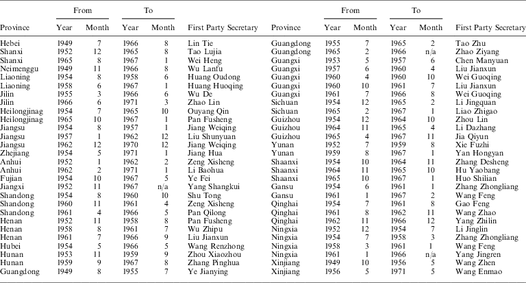
My main goal is to test whether AMs were more radical politically than FMs. The key independent variable of interest is therefore membership status, which is defined according to whether a provincial first party secretary was an FM, an AM or a nonmember (NM), using FMs as the reference group in the analysis.Footnote 9 As complications may arise if two party secretaries were found to serve in the same province in a given year, I employ the criterion adopted by Li and Zhou (Reference Li and Zhou2005) and select the party secretary who served on 30 June of that year as the representative leader of that province, and use her membership status accordingly. For instance, in Liaoning Province, Huang Oudong ended his tenure as the province's first party secretary in June of 1958, with Huang Huoqing replacing him immediately in the same month. While the precise date of this turnover is not specified, what is clear is that Huang Huoqing was in charge of Liaoning Province on June 30. Going by our rule, I choose Huang Huoqing (rather than his predecessor) to be the first party secretary of Liaoning Province for the year 1958.Footnote 10
Individual Characteristics of the First Party Secretary
Here I control for the age, years of party membership and “revolutionary credentials” (experience of the Long March is the pertinent proxy) of the provincial first party secretaries.Footnote 11 In the extension using the RD design, I also control for their education (as a measure of competence) and add a new variable, Anti-Japanese Military and Political University (AJMPU, or “Resistance University”), to check the robustness of their Long March credentials.Footnote 12 Since the AJMPU was the training ground for both military and political cadres of the CCP, I consider a province's first party secretary who was affiliated with the AJMPU—in the capacity of an administrator or instructor (or even a student)—as having significantly greater (revolutionary) credentials than those without such affiliations, and I construct a dummy variable to reflect that difference.Footnote 13 In addition to being a corroborating proxy, this broader categorization of the AJMPU should also permit a more encompassing definition of revolutionary credentials than the Long March.Footnote 14
Provincial Socio-economic Variables
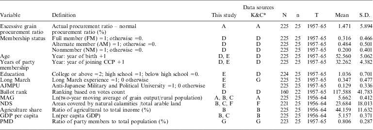
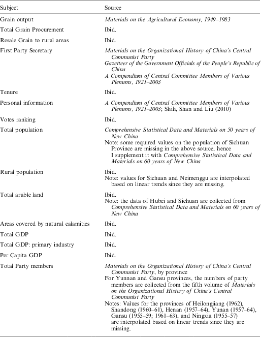
Going beyond the individual level, I control for the possible effects of food availability, natural calamities, share of agriculture and GDP per capita. While I define these variables in basically the same way as Kung and Chen (Reference Kung and Chen2011) do, to avoid reverse causality I lag these economic variables by one year, as excessive procurement in a given year may affect these socio-economic variables in the subsequent year. As for Party Membership Density (a proxy for local variations), instead of defining it as the ratio of the number of party members to the total number of cadres in a province (Kung and Chen Reference Kung and Chen2011), I change the denominator to a province's population, as there are simply too many missing observations based on the previous definition. Table 1 defines all the variables and data sources (see Appendix Table A1 for details of data construction).
Variables Definition and Data Sources
(1) N: observations; n: number of provinces; (2) Sources. A: Materials on the Agricultural Economy, 1949–83; B: Comprehensive statistical data and materials on 50 years of new China; C: Comprehensive statistical data and materials on 60 years of new China; D: A Compendium of Central Committee Members of Various Plenums, 1921–2003; E: Shih, Shan and Liu (2010); F: Report on China's Natural Disasters; G: Materials on the Organizational History of China's Central Communist Party. *Kung and Chen (Reference Kung and Chen2011).
Results of Fixed-Effects Estimates
Although I am using essentially the same variables and data as Kung and Chen (Reference Kung and Chen2011) to conduct the RD analysis, I replicate their results in part because of the slight modifications made to the period under analysis (now 1957–65) and the definition of variables (for example, Party Membership Density), and in part to correct for some data entry errors in the dependent variable Excessive Grain Procurement in their work. Doing so also allows me to establish a benchmark against which to compare the RD estimates. Following their empirical strategy, I employ a two-way fixed-effects model to test the relationship between membership status and political radicalism. The latter is measured by Excessive Grain Procurement, which is specified as:
 $$EP{{R}_{it}}\, = \,{{\beta }_1} \cdot A{{M}_{it}}\, + \,{{\beta }_{\rm{2}}} \cdot N{{M}_{it}}\, + \,{{X}_{it}}\gamma \, + \,{{Z}_{it}}\rho \, + \,{{\alpha }_i}\, + \,{{\lambda }_t}\, + \,{{\upsilon }_{it}},$$
where EPRit represents the excessive procurement ratio, AMit (or NMit) is a dummy variable indicating whether a provincial first party secretary is an AM (or NM), and FMs are the reference group in the analysis. Xit represents the individual characteristics of the provincial leaders, including age and years of party membership. Zit is a set of control variables, which include per capita food availability, level of natural calamities, GDP per capita, proportion of agricultural income and party member density. αi is the time-invariant and province-specific effect for province i, λt is the province-invariant and time-specific effect for year t and υit is the residual error term. My analysis covers the period 1957–65. I drop the municipalities of Shanghai, Beijing and Tianjin from the analysis, given their special administrative status, whereas Tibet is excluded due to the lack of systematic information on this autonomous region.Footnote 15 My analysis thus covers a total of 25 provinces, with a panel length of nine years for each province. The provincial party secretaries and their corresponding tenure details (with information on the exact months and years of their appointments) are shown in Appendix Table A2.
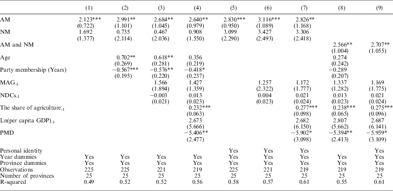
Based on the specification of Equation 1, I run two sets of regressions—the first without controlling for the “personality” fixed effects and the second with this important control. The other control variables are added to the regressions gradually. In Model 1, for instance, I include only the key variable of Membership Status, and in Model 2 the two control variables of the individual characteristics of the party secretaries are added. In Model 3, two more variables are added to further control for the provincial differences in grain output (Food Availability and Natural Disasters), whereas Model 4 takes into account the possible influence of both the differences in levels of economic development (GDP per capita, the proportion of agricultural income) and “local variations” (using Party Member Density as the pertinent proxy) across the provinces.
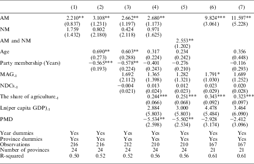
The first set of regression results is reported in the left panel of Table 2 (Columns 1–4). The results confirm the hypothesis that the AMs are significantly more radical than the FMs when it comes to grain procurement. Compared with the variable FM, the variable AM is highly significant (at the 1 percent level of significance in the baseline result, Column 1). Although the level of significance decreases somewhat (from 1 to 5 percent) as more control variables are added to the estimations (Columns 2–4), overall the results lend firm support to the hypothesis that membership status significantly affects the behavior of the provincial party secretaries. Moreover, the magnitude becomes larger in the full model (the pertinent coefficient increases from 2.123 in Column 1 to 2.640 in Column 4). In Column 4, the full model, age becomes insignificant, and the effect of party membership—which is negatively correlated with political radicalism—becomes only marginally significant, suggesting that these two individual characteristics are not good predictors of political behavior.
Fixed Effects Estimation of Membership Status and Personal Identities
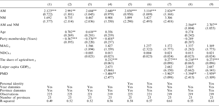
Note: robust standard errors in parentheses. *significant at 10%; **significant at 5%; ***significant at 1%. Constant terms are included but not reported.
The right panel of Table 2 (Columns 5–7) reports the regression results after controlling for the personal identities of provincial leaders serving as first party secretaries (each dummy variable indicates the exact identity of the first party secretary of a given province for the period under analysis). The results show that the variable AM remains significant at the conventional levels of significance ranging from 1 to 5 percent, with larger magnitudes than the previous estimates. For instance, a comparison of the two full models reveals that the coefficient of AM increases from 2.640 (Column 4) to 2.826 (Column 7). These results robustly reaffirm Kung and Chen's (2011) key hypothesis that political radicalism varied systematically according to the status of CC membership even after controlling for the effect of “personality.”
To see if this hypothesis still holds in the event that the NMs were just as radical as the AMs (for they too may arguably be anxious to get promoted to AM and would therefore act radically), I combine NMs and AMs into the same category and compare them as a group against the FMs. Reported in Columns 8 and 9, the results show that there are still significant differences in the degree of radicalism between these different political categories.Footnote 16
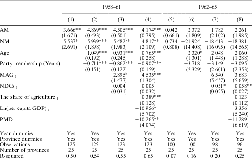
An important question, however, remains. The radical phase of the Great Leap Forward was before 1958–61, but our analysis covers also the period 1962–65. Would the analytical results change if we shorten our period of analysis? To find out, I subdivide the sample into the two shorter periods, before 1962 and after 1962, and repeat the same exercises. The results reported in Appendix Table A4 robustly show that AMs are still significantly more radical than FMs before 1962 and the magnitude is even larger (for example, 4.174, Column 4) than the baseline estimate of 2.640 (Column 4 in Table 2). By contrast, the difference is not significant in the post-Great Leap Famine period.
Determinants of CC Membership Ranking and Mao's Influence: Bases For The RD Design
There are two primary reasons for employing the RD design to analyze the role of political career incentives in possibly causing excessive political radicalism during China's Great Leap Forward. First, instead of analyzing the average effect of membership status (of the AMs as a group vis-à-vis the FMs as a group) on political radicalism, our specific hypothesis entails the analysis of the marginal effects—those that capture the difference in the degree of radicalism between AMs and FMs who rank near the discontinuous threshold. Clearly this entails an analysis of an RD design (see section below).
The other justification for employing an RD design is premised on the well-documented evidence of Mao's conscious efforts to fuel provincial leaders’ incentives to comply with the Leap's goals, as these stimuli may have changed the “personal idiosyncrasies” of these leaders either shortly before or during the Leap.Footnote 17 The RD design, which relies on exploiting the variation in the ballot-determined ranking of the CC members, should help address the concern of this possible omitted variable bias.
A Congressional Ballot Outcome and CC Membership Ranking
Just as Thistlethwaite and Campbell (Reference Thistlethwaite and Campbell1960) analyze the impact of merit awards on future academic outcomes, here I study the possible effect of CC membership status on radical political behavior—specifically excessive grain procurement. Following their central idea—that individuals who ranked just below a certain cutoff point for an award (that is, those who just missed out on an award) serve as good comparisons for those who ranked just above the cutoff value (that is, those who just exceeded the threshold for an award)—I assume that the AMs who ranked near the cutoff point for full CC membership status were good comparisons to the FMs who also ranked near that cutoff point. To prove that this context satisfies the RD requirement that the individuals concerned were unable to precisely sort themselves around the discontinuity threshold (that is, to assign a particular membership status to themselves, say FM), I first provide a descriptive analysis of the pertinent institutional context, specifically the mechanisms for generating membership rankings. I then explain the paradox of why, in spite of this rigid institutional feature, the AMs were more radicalized by their desperate desire for promotion than the FMs, who could not hope to advance much further.
Although beginning in around the late 1950s Mao was increasingly behaving like a dictator,Footnote 18 the CCP had already developed formal political institutions governing membership, protocol, etc., as well as a set of formal rules and procedures designed to “both facilitate the exchange of information among the ruling elites and provide for an easy assessment of compliance with those rules” (Svolik Reference Svolik2012, 7; see also MacFarquhar Reference MacFarquhar1997). Given the political importance of the CC-CCP, there was an elaborate procedure for: (1) governing membership eligibility; (2) determining, by voting, the relative rankings of those who are eligible; and (3) specifying a precise cutoff point that effectively divides the CC members into two classes—FMs and AMs. These procedures made it virtually infeasible for the eligible nominees to manipulate the voting to the extent of influencing the final ranking, which determined membership status.
In a nutshell, a total of 1,026 delegates competed for one of 170 seats on the CC.Footnote 19 The 170 finalists were chosen only after three rounds of voting. After the first round of voting, a revised list was presented to the delegates, who were then asked to conduct another round of voting. Those voted on in the second round were then presented to the delegates again for a final secret ballot, in which each of the 1,026 delegates was given a form that contained the names of the 170 nominees who made it through the first two rounds. The pertinent instruction, for these delegates, was to strike out the names of those they did not support for a place in the CC. Unless a nominee was rejected by all 1,026 delegates, his place on the CC was now assured and his ranking determined based on the outcome of this third and final round.Footnote 20
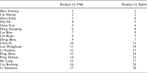
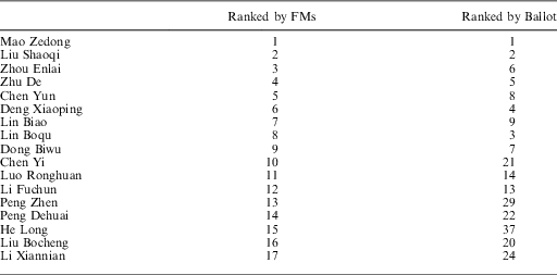
As each eligible nominee could be voted on more than once, and although the 170 finalists would most certainly have lobbied the Congress delegates to vote for them, it is unlikely that they were able to precisely influence the number of votes they each received to the extent of affecting their eventual CC ranking (and accordingly, their membership status). In fact, with the sole exception of Mao, even the top leadership would have found it a formidable task to control the number of votes to the extent of tallying the ballot outcome with that of their own preference.Footnote 21 At least that appeared to be the case for the Politburo. For example, with the exception of Mao Zedong and Liu Shaoqi, the “internal” rankings of the other 15 Politburo members all differed from the ballot outcome (Appendix Table A5). This particular mechanism of determining CC membership ranking (and, accordingly, the assignment of members to either FM or AM status) thus prevents individual CC members from precisely sorting themselves around the discontinuity threshold; this feature importantly qualifies the analysis for an RD design.Footnote 22
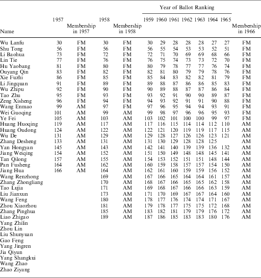
Another distinctive feature of the mechanism of determining membership ranking is that, once the members’ rankings were determined by the final ballot outcome, future changes in ranking became automatic: one would automatically move up the rank upon the death of a more senior member, and would be promoted to full membership after crossing the threshold that separates FMs from AMs. A CC member would thus become an FM upon coming 97th (or higher) in the rankings. This was the case, for example, of Wang Enmao, the first party secretary of Xinjiang Province. Ranked 99th on 30 June 1957, Wang moved up two notches to rank 97th a year later and was promoted to FM, thanks to the deaths of two FMs.Footnote 23 Similarly, Ye Fe, the first party secretary of Fujian Province (who ranked 103rd in 1958) advanced six notches by 1966 to rank 97th upon the demise of six FMs during this period and was thus promoted to full membership that year.Footnote 24 The ballot results for all CC members who held the first party secretary position between 1956 and 1966 are summarized in Appendix Table A6 (and presented visually in Figure 2), which shows that a CC member indeed qualified for full membership upon coming 97th in the rankings. In short, this automatic feature of membership movement prevents individuals from rigging the votes and affecting the ranking accordingly.
The relationship between ballot ranking and membership status
Figure 2 previews the discontinuity in membership status by plotting the bivariate relationship between Membership for the 1957–66 period and Ballot Ranking—our assignment variable. The fitted values, which are obtained from nonparametric regressions using Cleveland's (Reference Cleveland1979) tricube weighting function and a bandwidth of 0.5, are estimated separately for observations on either side of the cutoff value. The fitted values may thus be considered to represent the moving average of membership status across the entire range of ballot rankings; the scattered data points (hollow squares and circles) represent the membership of individual CC members. Figure 2 clearly shows that there is a discontinuity in membership status at the thresholds.
If advancement through the ranks was mechanically determined by what was essentially the natural attrition of the FMs, does it not contradict our central thesis regarding the differential incentives between AMs and FMs whose rank was close to the discontinuity threshold? The answer is no. The differential incentives between the two membership statuses stem from the fundamental fact that the probability that an AM will acquire the higher status of FM at the next congressional meeting is smaller than the probability that an FM will retain the same status. This difference thus provided sharp enough incentives for the AMs to exert greater efforts during the Leap in the hope of gaining more votes at the next congressional ballot. Moreover, the fact that nobody knew just when the next congressional session would take place helped create the expectation (illusion) that promotion could come sooner than the “constitutional” rule dictated.Footnote 25
Mao's Influences and Possible Omitted Variable Bias
While Kung and Chen (Reference Kung and Chen2011) controlled for the omitted variable of personal identities in their fixed-effects estimations, the “personalities” or political dispositions of provincial leaders may change over time in response to Mao's persuasions. As Mao became increasingly impatient with the slow pace of economic development (for which he blamed the cautiously “expert” approach of the planners),Footnote 26 he took a number of carefully orchestrated steps to persuade the provincial leaders—the actors Mao relied upon the most to spur the Leap—to increase production targets. For instance, at a number of ad hoc conferences that Mao set up and enlisted the unprecedented participation of the provincial leaders,Footnote 27 he attended only those sessions presided by the local leaders (Teiwes and Sun Reference Teiwes and Sun1999). Moreover, of the dozen or so provincial party secretaries who accompanied Mao during his campaign tours in 1958, half were FMs; as many as four of them ranked just above 97 in the CC and one was exceptionally inducted into the Politburo in the same year (see below).Footnote 28
As long as some provincial leaders responded to this deliberate act of Mao in the way he intended, the fixed-effects estimation would fail to account for the effect of this possible influence—one that potentially affects both career incentives and political radicalism simultaneously. By exploiting the variation in CC membership ranking determined by congressional ballot—which is uncorrelated with personality but which can affect membership status, the RD design serves to identify the latter's causal effect on political radicalism, thereby correcting for the possible omitted variable bias (of “personality change”) arising from the provincial leaders’ interactions with, and their differential responses to, Mao in the fixed-effects model.
A Regression Discontinuity Design
Model Specifications
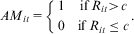
Given that membership status (AMit) is automatically determined (discontinuously) by a member's ranking (Rit), I employ the sharp RD design to exploit its effect on political radicalism, conditional upon ranking (Rit). Specifically, given that the discontinuous jump in the status of CC membership occurs at the cutoff point c of 97, we have
 $$A{{M}_{it}}\, = \,\left\{ \matrix { {\rm{1}} & {{\rm{if}}\,{{R}_{it}} \gt c} \cr{\rm{0}} & {{\rm{if}}\,{{R}_{it}}\leq c} \\\end{}} \right..$$
To allow for an easier interpretation of the empirical results, I normalize ranking as a function of  $$$ {{r}_{it}}\, = \,\frac{{{{R}_{it}}\,{\rm{ - }}\,c}}{c} $$$
, which allows the function of membership status to be written as:
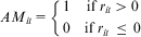 $$A{{M}_{it}}\, = \,\left\{ \matrix {{\rm{1}} & {{\rm{if}}\,{{r}_{it}}\, \gt \,{\rm{0}}} \cr{\rm{0}} & {{\rm{if}}\,{{r}_{it}}\,\leq \,0} \\\end{}} \right.$$
and the RD estimates to be constructed as:
 $$\matrix {{EP{{R}_{it}}} \hfill & {\, = \,A{{M}_{it}}EP{{R}_{it}}(1)\, + \,(1\,{\rm{ - }}\,A{{M}_{it}})EP{{R}_{it}}(0)} \hfill \cr\ {} \hfill & {\, = \,\left\{ \matrix {{EP{{R}_{it}}(1)} \cr{EP{{R}_{it}}(0)} \\\end{}} \right. = \left\{ \matrix{{\beta \cdot 1\, + \,{{f}_{\rm{1}}}({{r}_{it}})\, + \,{{X}_{it}}\gamma \, + \,{{Z}_{it}}\rho \, + \,{{\alpha }_i}\, + \,{{\lambda }_t}\, + \,{{\upsilon }_{it}}} & {{\rm{if}}\;{{r}_i}\, \gt \,{\rm{0}}} \cr{\beta \cdot 0\, + \,{{f}_{\rm{0}}}({{r}_{it}})\, + \,{{X}_{it}}\gamma \, + \,{{Z}_{it}}\rho \, + \,{{\alpha }_i}\, + \,{{\lambda }_t}\, + \,{{\upsilon }_{it}}} & {{\rm{if}}\;{{r}_i}\,\leq \,{\rm{0}}} \\\end{}} \right} \hfill \\\end{}}.$$
Assuming that f 0 (rit) and f 1 (rit) are continuous in the neighborhood of zero (a standard assumption of the RD design), we can also rewrite Equation 3 as:
 $$EP{{R}_{it}}\, = \,\beta \cdot A{{M}_{it}}\, + \,{{f}_1}({{r}_{it}})\, + \,[{{f}_1}({{r}_{it}})\,{\rm{ - }}\,{{f}_0}({{r}_{it}})] \cdot A{{M}_{it}}\, + \,{{X}_{it}}\gamma \, + \,{{Z}_{it}}\rho \, + \,{{\alpha }_i}\, + \,{{\lambda }_t}\, + \,{{\upsilon }_{it}}.$$
Figure 3 visually previews the RD results by plotting the bivariate relationship between the degree of radicalism for the period 1957–65 and ballot ranking. As explained earlier, the fitted values are obtained from nonparametric regressions using Cleveland's (Reference Cleveland1979) tricube weighting function and a bandwidth of 0.5 estimated separately for observations on either side of the cutoff value.Footnote 29 The fitted values thus represent the moving average of excessive grain procurement across the entire range of ballot rankings; the scattered data points represent the various levels of political radicalism of individual CC members. Figure 3 presents clear evidence that the AMs tended to procure more grain.Footnote 30 An especially convincing feature of the graph is that it provides clear evidence of a discontinuous increase in grain procurement at the juncture ri=0. This jump is meaningful, as it seems improbable for other determinants of grain procurement to change as suddenly at the cutoff point as membership status.Footnote 31
The relationship between ballot ranking and excessive grain procurement ratio
Now turning to the estimations, although nonparametric techniques are advantageous in that they do not rely on the assumption of functional forms, the small size of our sample obligates us to employ parametric estimations instead. As Lee and Lemieux (Reference Lee and Lemieux2010) suggest, a simple way of relaxing the linearity assumption in parametric estimations when the true functional form is unknown is to “include polynomial functions of X in the regression model” (316). We thus model f 0 (rit) and f 1 (rit) as functions with varying degrees of polynomials, and rewrite Equation 3 as:
 $$\matrix {{E(EP{{R}_{it}}|A{{M}_{it}}\, = \,0)} \hfill & {\, = \,{{\psi }_{01}}{{r}_i}\, + \,{{\psi }_{02}}r_{i}^{2} \, + \, \cdots \, + \,{{\psi }_{0p}}r_{i}^{p} \, + \,{{X}_{it}}\gamma \, + \,{{Z}_{it}}\rho \, + \,{{\alpha }_i}\, + \,{{\lambda }_t}\, + \,{{\upsilon }_{it}}} \hfill \cr{E(EP{{R}_{it}}|A{{M}_{it}}\, = \,1)} \hfill & {\, = \,{{\psi }_{11}}{{r}_i}\, + \,{{\psi }_{12}}r_{i}^{2} \, + \, \cdots \, + \,{{\psi }_{1p}}r_{i}^{p} \, + \,{{X}_{it}}\gamma \, + \,{{Z}_{it}}\rho \, + \,{{\alpha }_i}\, + \,{{\lambda }_t}\, + \,{{\upsilon }_{it}}} \hfill \\\end{}$$
and the regression model as:
 $$EP{{R}_{it}} = \beta \cdot A{{M}_{it}}\, + \,\mathop{\sum}\limits_{j\, = \,{\rm{1}}}^P ({{\kappa }_{0j}}r_{{it}}^{j} \, + \,\kappa _{j}^{\ast} r_{{it}}^{j} A{{M}_{it}})\, + \,{{X}_{it}}\gamma \, + \,{{Z}_{it}}\rho \, + \,{{\alpha }_i}\, + \,{{\lambda }_t}\, + \,{{\upsilon }_{it}},$$
where  $$${{\kappa }_{0j}} = {{\psi }_{0j}}$$$
and
 $$$\kappa _{j}^{\ast} \, = \,{{\psi }_{1j}}\,{\rm{ - }}\,{{\psi }_{0j}}$$$
. In the case of polynomial regressions, the key question concerns the choice of the order of the polynomial regressions, which can be decided using the Akaike information criterion (AIC) of model selection. In the RD context, AIC is given by
 $$$nln({{\mathop{\sigma }\limits^{\frown}}^2} ) + 2(P + 1)$$$
, where
 $$$\mathop{\sigma }\limits^{\frown}$$$
is the mean squared error of the regression and P is the number of parameters in the regression model (order of the polynomial) (Lee and Lemieux Reference Lee and Lemieux2010). The AIC can be minimized by choosing P.
Empirical Results
Baseline results
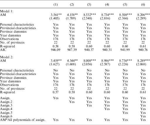
Model 1 of Table 3 (the upper panel) examines the robustness of the polynomial rit by means of six specifications. Columns 1–6 report the results that include AMit, the first through to the sixth-order polynomials of rit, and the interactions between AMit and the polynomials of various orders—linear (P=1), quadratic (P=2), cubic (P=3) and so on. We also report the AIC statistics for all the specifications. The optimal order of polynomial, which can be decided by minimizing the AIC, is four, implying that it is necessary to control for the quartic polynomial and its interactions with AMit. That the fourth-order polynomial is optimal can easily be seen from the fact that the AIC that controls for the cubic polynomials and their interactions with AMit (Column 3) is only trivially larger (by implication of the AIC) than the one controlling for a higher-order polynomial (Column 4), and that the estimated effects of AMit are strikingly similar between these two specifications. Conversely, the models with lower-order polynomials are suboptimal because they result in significantly smaller estimates and larger AICs (Columns 1 and 2). Overall, the robustness of our estimations is borne out by the fact that AMit continues to exhibit a highly significant and positive effect on the excessive grain procurement ratio even in estimations that include higher-order polynomials and their interactions with AMit (Columns 5–6), suggesting that our results are not sensitive to the order of the polynomial. In terms of magnitude, the RD estimate yields a coefficient of 8.734 (Column 4, Table 3)—more than three times the estimate of the fixed-effects model (2.826, Column 7, Table 2). To verify that these results are not confounded by the individual characteristics of the provincial leaders, I dropped all the personal characteristics in Model 2 (Table 3), and found that the results changed only trivially (compare, for example, the coefficient of 8.986 with 8.734 in Column 4 of the two models)—the former is larger by a mere 0.25.
Regression Discontinuity Estimations of Alternate Members’ Political Radicalism
Note: robust standard errors in parentheses. *significant at 10%; **significant at 5%; ***significant at 1%. Constant terms are included but not reported. Control variables include all control variables in Column 4 of Table 2.
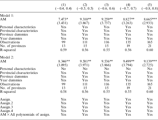
Given that the RD results may be sensitive to the choice of bandwidth, I replicate our estimations using different bandwidths to ensure that our baseline results are robust.Footnote 32 I do so by using the alternative bandwidths of (−0.4,0.4), (−0.5,0.5), (−0.6,0.6), (−0.7,0.7) and (−0.8,0.8), based on the specification in Column 4 of Table 3 (Model 1). These checks show that the estimates do not change systematically with the change in bandwidth. In particular, compared with the estimates based on the whole sample (8.734 in Column 4 of Table 3), the magnitudes of the coefficient (of AM) fall within a remarkably close range of that using the original bandwidth (see Appendix Table A7 for details).
Robustness check
A concern arises, however, if the probability of receiving the treatment does not change from 0 to 1 at the threshold, in which case we need a design that allows for a smaller jump in the probability at the threshold (Imbens and Lemieux Reference Imbens and Lemieux2007). Table A6 indeed shows that “compliance” with the institutional rules and mechanisms is less than perfect—that is, while some AMs were already ranked 97th before 1966 (for example, Wei Guoqing in 1961 and Ye Fei in 1965), they did not officially become FMs until August 1966 (the 9th National Congress). This time lag before an individual was granted full membership implies that the treatment in question is less than 1 (ri ≤ 0), which suggests that it is necessary to check the robustness of our previous estimates using the fuzzy RD design.Footnote 33 We thus assume in this context that the probability of being an AM is smaller than 1, as specified in Equation 6:
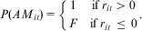 $$P(A{{M}_{it}})\, = \,\left\{ \matrix {{\rm{1}} & {{\rm{if}}\,{{r}_{it}}\, \gt \,0} \cr F & {{\rm{if}}\,{{r}_{it}}\,\leq \,0} \\\end{}} \right..$$
We also assume that alternate membership can be written as:
 $$E(A{{M}_{it}})\, = \,\phi \cdot {{D}_{it}}\, + \,\mathop{\sum}\limits_{j\, = \,{\rm{1}}}^P ({{\varphi }_{0j}}r_{{it}}^{j} \, + \,\varphi _{j}^{\ast} r_{{it}}^{j} {{D}_{it}})\, + \,{{X}_{it}}\rOmega \, + \,{{Z}_{it}}\theta \, + \,{{\alpha }_i}\, + \,{{\lambda }_t},$$
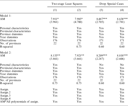
where Dit is a dummy variable indicating a ranking lower than the cutoff value, namely ri > 0. The most straightforward method of estimating Equation 7 is to regress AMit on Dit and a set of control variables first, followed by regressing the excessive procurement ratio on the predicted values of AMit and the same set of control variables. The results are reported in Table 4. Specifically, AMit remains significant after controlling for the cubic and quartic polynomials and their interactions with AMit (Columns 1 and 2). Their magnitudes, which are bound between 7.911 and 7.985, are only slightly smaller than the baseline results of 8.532 and 8.734 (Columns 3 and 4 in Table 3). As Ye Fei and Wei Guoqing were not promoted until several years after they reached the threshold (see Table A6), to ensure that our results are not driven by these two special cases I dropped them from the analysis. Columns 3 and 4 of Table 4, which reports these alternative results, show that the effect of AMit now becomes 8.638, which is strikingly similar to the pertinent coefficient of 8.734 in Table 3 (Column 4). The result of the fuzzy RD estimation thus confidently reaffirms the baseline results.
Regression Discontinuity Estimations: Robustness Checks
Note: robust standard errors in parentheses. *significant at 10%; **significant at 5%; ***significant at 1%. Constant terms are included but not reported. Control variables include all control variables in Column 4 of Table 2.
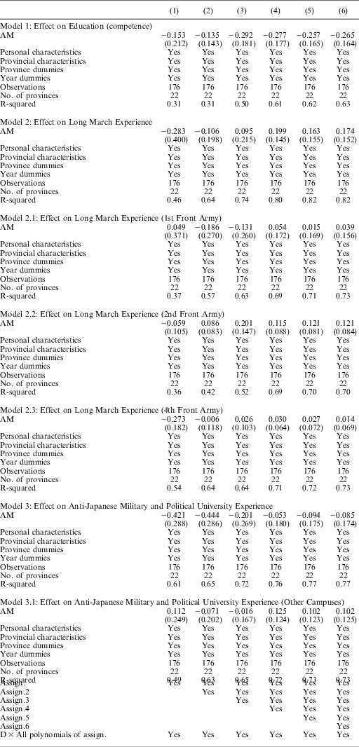
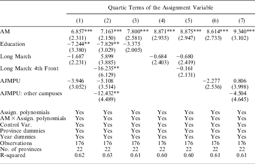
The RD approach requires the identifying assumption that, except for the assignment variable, all outcomes must vary smoothly at the cutoff point (that is, they have to be continuous). Suppose W 1 and W 0 represent the potential outcomes in the two groups with AMit=1 and AMit=0, respectively. Then E (W 1 | x,Z) and E (W 0 | x,Z) must be continuous at the cutoff point. I evaluate this assumption in the Appendix, and find that AMit is uncorrelated with any of the control variables including Age, Years of Party Membership, Education (a proxy for competence), and Long March Experience and AJMPU (proxies for revolutionary credentials) (see Table A8). Moreover, even with the inclusion of Education, Long March Experience and AJMPU, the effect of AMit remains highly significant (see Appendix Table A9).Footnote 34
Placebo test
Although the above robustness check confirms that membership status has no significant effect on Wi (comprising age, years of party membership, and education and revolutionary credentials), and that it remains significant even after controlling for these variables, there may still be other unobserved changes around the cutoff value. To rule out this possibility, I perform a placebo test by changing the discontinuity threshold.Footnote 35 If doing so does not alter our previous results, we can be more confident of our RD estimates. We assume, for instance, that the discontinuous jump in the status of CC membership occurs at points other than 97. We then have
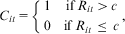 $${{C}_{it}}\, = \,\left\{ \matrix {{\rm{1}} & {{\rm{if}}\,{{R}_{it}}\, \gt \,c} \cr{\rm{0}} & {{\rm{if}}\,{{R}_{it}}\,\leq \,c} \\\end{}} \right.,$$
in which I assume that c=90,93,…96 and 98,99, …104. Similarly, I normalize ranking as a function of  $$${{r}_{it}}\, = \,\frac{{{{R}_{it}}\,{\rm{ - }}\,c}}{c}$$$
, which allows the function of membership status to be written as
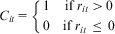 $${{C}_{it}}\, = \,\left\{ \matrix {{\rm{1}} & {{\rm{if}}\,{{r}_{it}}\, \gt \,{\rm{0}}} \cr{\rm{0}} & {{\rm{if}}\,{{r}_{it}}\,\leq \,{\rm{0}}} \\\end{}} \right.$$
and the RD estimates to be constructed as
 $$EP{{R}_{it}}\, = \,\beta \cdot {{C}_{it}}\, + \,\mathop{\sum}\limits_{j\, = \,1}^P ({{\kappa }_{0j}}r_{{it}}^{j} \, + \,\kappa _{j}^{\ast} r_{{it}}^{j} {{C}_{it}})\, + \,{{X}_{it}}\gamma \, + \,{{Z}_{it}}\rho \, + \,{{\alpha }_i}\, + \,{{\lambda }_t}\, + \,{{\upsilon }_{it}}.$$
I plot the estimates of β in Figure 4 along the x-axis according to different thresholds. The results show that the effect of other cutoff values is not significant: only discontinuity at the cutoff point of 97 has a significant effect on grain procurement, which suggests that the RD approach does capture the effect of the membership assignment rule instead of other unobserved changes. To check the robustness of this result, I further assume that c takes on other, more extreme, values—specifically 60, 75, 119 and 134. The results show that the effects of these arbitrary cutoff values are not significant. Moreover, for cutoff values that are substantially smaller than 97 (for example, 60), the standard deviation becomes considerably larger due to the drastically reduced number of observations around this cutoff value.
Placebo test: effect of changing the discontinuity threshold
Effects of Career Incentives on Those Ranking Near The Threshold
The Discontinuous Jump in Political Radicalism between AMs and FMs
A unique feature of the RD design is that, instead of measuring the average effect of the explanatory variable on the dependent variable, it measures the marginal effects, because RD is concerned with the effects of only those values lying around the discontinuous threshold. This can be illustrated by Equation 9, which is rewritten from Equation 5:
 $$\matrix { {EP{{R}_{it}}} \hfill & {\, = \,\overline{\beta } \cdot A{{M}_{it}}\, + \,\mathop{\sum}\limits_{j\, = \,1}^P {{\kappa }_{0j}}r_{{it}}^{j} \, + \,{{X}_{it}}\gamma \, + \,{{Z}_{it}}\rho \, + \,{{\alpha }_i}\, + \,{{\lambda }_t}\, + \,{{\upsilon }_{it}}} \hfill \cr{} \hfill & {\, = \,\left( {\beta \, + \,\mathop{\sum}\limits_{j\, = \,1}^P \kappa _{j}^{\ast} r_{{it}}^{j} } \right)A{{M}_{it}}\, + \,\mathop{\sum}\limits_{j\, = \,1}^P {{\kappa }_{0j}}r_{{it}}^{j} \, + \,{{X}_{it}}\gamma \, + \,{{Z}_{it}}\rho \, + \,{{\alpha }_i}\, + \,{{\lambda }_t}\, + \,{{\upsilon }_{it}}} \hfill \\\end{}}.$$
While the fixed-effects model (first line in Equation 9) estimates  $$$\bar{\beta }$$$
without controlling for any polynomials of the assignment variable,Footnote 36 the RD measures, in this instance, the effect of membership status (allocated on the basis of ballot ranking) around the threshold that separates the AMs from the FMs, β, on excessive grain procurement (second line in Equation 9). This explains why the magnitude of AMit, according to the RD estimate (8.734, Column 4, Table 3), is so much larger than the fixed-effects estimate (2.826, Column 7, Table 2).
To illustrate this unique property of the RD design in our context of interest, I plot the coefficients of the term  $$$\bigg(\big(\beta \, + \,\mathop{\sum}\nolimits_{j\, = \,1}^P \rho \kappa _{j}^{\ast} r_{{it}}^{j} \big)A{{M}_{it}} + \mathop{\sum}\nolimits_{j\, = \,1}^P \kappa _{{0j}}^{\ast} r_{{it}}^{j} \bigg)$$$
in Figure 5 based on the results in Table 3 (Column 4). The x-axis measures the ballot ranking of the CC members using the normalized term
 $$$\frac{{{{R}_{it}}\,{\rm{ - }}\,c}}{c}$$$
, whereas the y-axis measures the degree of radicalism. The solid, vertical line in the middle represents the cutoff point that separates AMs and FMs; specifically, it represents the degree of radicalism of the AMs to the right and the degree of radicalism of the FMs to the left. A striking feature of Figure 5 is that political radicalism experiences a discontinuous jump as the ballot ranking turns from positive (to the right of the vertical line) to negative (to the left)—a feature that confirms that the difference in the degree of political radicalism between FMs and AMs is driven by the difference in membership status.Footnote 37
Degree of political radicalism, by ballot ranking
Specifically, Figure 5 reveals that, in the case of AMs, those who came closest to the cutoff point (of 97) are indeed the most radical. Being on the verge of promotion, these CC members hardly needed any persuasion from Mao to toe his line. But radicalism declines in tandem with the decrease in ranking (reflected in the increase in ballot ranking), suggesting that those with significantly lower rankings saw little hope of promotion. In sharp contrast to the highest-ranked AMs, FMs who only just made it are the least radical, for they must have anticipated only a small likelihood of promotion to the Politburo and so had distinctly weaker incentives to procure more grain. Consistent with the logic discussed earlier, however, radicalism rises in tandem with ranking. These patterns of relationship are highly robust: the shapes of the curves are strikingly similar regardless of the order of the polynomials (cubic and quartic) used.
Countering Political Complacency: Mao Strikes Back
Our findings so far are seemingly inconsistent with the fact that the best-known Leap radicals (the so-called four radical kings: Li Jingquan (ranked 89 in 1958) of Sichuan Province, Ke Qingshi (35, an exception to being a lowly ranked FM) of Shanghai, Wu Zhipu (90) of Henan Province and Zeng Xisheng (94) of Anhui Province—were all FMs.Footnote 38 Moreover, while these “radical kings” were indeed ranked just above the cutoff point in 1958, they were anything but passive watchers of the Leap. Yet it takes more than half a dozen zealous provincial leaders to fire all the cylinders of the Leap. Realizing that many of these leaders, if left to themselves, would likely have rested on their laurels, Mao exercised his exceptional authority and bent the rules of the promotion system in order to more effectively influence and manage the political incentives of China's provincial leaders.Footnote 39
Take Li Jingquan of Sichuan Province, for instance. Although Li managed to climb up the rankings from 91st in 1956 to 89th two years later (by dint of the autopilot mechanism), he was nowhere near the rankings normally needed to be considered for promotion to the Politburo. Li was promoted in May 1958 in part to reward his past efforts and loyalty, but perhaps more importantly because Mao, who had the power to exceptionally promote zealous officials regardless of their ranking, wanted to motivate other lowly ranked FMs to pull their acts together. More importantly, Li's promotion was not done in isolation, but arranged jointly with two other radicals—Ke Qingshi (ranked 35th) and Tan Zhenlin (ranked 69th)—which would have sent a loud and clear message to the less-motivated FMs that loyalty to Mao would be duly rewarded. The importance of promoting Li was also noted outside of Sichuan Province, because, in addition to being the first party secretary of Sichuan, he was also in charge of the Southwest bureau apparatus (Xinan Ju), which included the provinces of Yunnan and Guizhou. Li's extraordinarily radical behavior in spearheading the Leap had likely put enormous pressure on the leaders of the other two provinces to keep up.Footnote 40
Wu Zhipu of Henan Province is another case in point. Although Wu, who ranked 90th in 1958 (just behind Li), was not as lucky as his Sichuan counterpart, he was still “promoted” from second (i.e., governor) to first party secretary, similarly shortly before the launching of the Great Leap. His otherwise trivial political ascendancy takes on unusual importance in the Leap's context, because Mao had designated Henan Province the “national model” province against which all other Chinese provinces should compare themselves.Footnote 41
Conclusion
A distinguishing hallmark of China's Great Leap Famine, the worst man-made famine in history, is that excess death rates were highly correlated with the political attitudes of the provincial leaders, which varied enormously across the country. Recent work suggests that, instead of attributing such variations to personal idiosyncrasies, a more fruitful approach is to make sense of the observed variations in political radicalism by examining the varying strengths of career incentives embedded in the structure of China's nomenklatura system (Kung and Chen Reference Kung and Chen2011). By exploiting the discontinuity in the assignment of AM vs. FM membership status to identify its causal effect on political radicalism using an RD design, I showed that the fixed-effects model grossly underestimated the effect of membership status by more than three times. This enormous difference can be attributed to the fact that the RD estimator measures only the differences in political radicalism between those AMs and FMs who ranked close to the discontinuous threshold, and thus captures the marginal rather than average effects between the two discrete groups. The RD results do show that there is a sudden jump in political radicalism as the ballot ranking crosses the cutoff value, or as membership changes from AM to FM.
Although my finding that the lowest-ranked FMs were the least radical may contradict the fact that the best-known radicals belonged to just such a category, I pointed out the lesser-known fact that at least one of the four best-known radicals had been exceptionally promoted to the Politburo in spite of his low ranking. A reasonable conjecture of this important decision is that Mao may have used these unusual promotions to counteract the rigid autopilot mechanism of the promotion system so that FMs who otherwise had little expectation of promotion (and, accordingly, weak incentives to fuel the Leap) could be stimulated into action. Moreover, given that the variation in the ballot ranking of the CC members is uncorrelated with “personality” (while clearly correlated with membership status), the RD design also helps to correct for the omitted variable bias resulting from the dictator's intended influence on the political dispositions of some local leaders.
In a context in which the Leap's success crucially depended on the efforts of the provincial leaders, and where the most powerful tool at the dictator's disposal to spur the leaders on was promotion and other high-powered incentives, it is difficult to imagine how political career incentives were not an important cause of the extraordinary political radicalism witnessed during this politically tumultuous episode of an authoritarian China (just as they were a primary determinant of the extraordinary economic performance during the last 30 years).
Appendix
Construction of Dataset
The First Party Secretaries of the Sample Provinces
Robustness Check (Excluding Xinjiang Province)
Robustness Check: Subdividing the Sample between 1958–61 and 1962–65
Rankings of Politburo Members, Internally Ranked Versus Ballot Ranked
Rankings (Based on Ballot) of the Provincial Leaders in the Central Committee of the Chinese Communist Party, 1956–66
Robustness Check: Regression Discontinuity Estimations Using Different Bandwidths
Testing RD Validity
Controlling for Competence and Revolutionary Credentials
Comparing Nonparametric and Parametric Estimations
The sharply larger coefficient obtained from the parametric estimations raises the concern that this result may be driven by functional form assumptions, even though I have already controlled for varying degrees of polynomials. One plausible reason for the large difference is that the province- and time-specific effects have not been controlled for in the nonparametric estimations. To see whether that is indeed the case, I replace the excessive procurement ratio with the predicted error term based on Equation 1 (that is, without the inclusion of AM) and regress it on the membership status of AM, the quartic and cubic polynomials (which have the smallest AIC), and their interactions as in the following equation:
 $$Erro{{r}_{it}}\, = \,\beta \cdot A{{M}_{it}}\, + \,\mathop{\sum}\limits_{j\, = \,1}^P ({{\kappa }_{0j}}r_{{it}}^{j} \, + \,\kappa _{j}^{\ast} r_{{it}}^{j} A{{M}_{it}})\, + \,{{\upsilon }_{it}}.$$
The effect of AM is 2.461 in the case of the quartic polynomials and 2.065 in the case of the cubic polynomials, which is much smaller than the results in which province- and time-specific effects are controlled for (Columns 3 and 4 in Table 2). The pertinent coefficient becomes sharply lower with such controls, because some provinces are likely more important than others, and in these provinces the first party secretaries tended to be FMs. Hence including the fixed effects drastically alters the size of AM's coefficient. To prove that there is no major difference between the nonparametric and parametric estimation results, I plot the predicted Errorit term (the grey dotted line) over the nonparametric results (the solid black line in Figure 3) in Figure A1.
Nonparametric Versus parametric estimations of the relationship between ballot ranking and excessive grain procurement ratio
Bandwidth Selection
Reported in Columns 1 to 5 of Table A7, the robustness checks begin with a relatively narrow bandwidth to one that covers nearly the entire range. While estimates based on very wide bandwidths (0.7 or 0.8) are larger than those that rely on the narrowest bandwidth (0.4), they are smaller than the ones that use bandwidths in the middle (0.5 or 0.6), suggesting that the estimates do not change systematically with the change in bandwidth. More importantly, compared with the estimates based on the whole sample (8.734 in Column 4 of Table 3), the magnitude of the coefficient (of AM) does not change significantly (ranging from 7.473 to 9.310) across the various bandwidths. As I have shown in Table 3, I am able to confirm that the results remain stable even when I omit the personal characteristics (Model 2)—they are strikingly similar to those of Model 1. Together, these robustness checks show that the baseline results are not sensitive to bandwidth selection.
Testing the Validity of the RD Design
Suppose W 1 and W 0 represent the potential outcomes in the two groups with AMit = 1 and AMit = 0, respectively, then E (W 1 | x, Z) and E (W 0 | x, Z) must be continuous at the cutoff point. To evaluate this assumption, I examine a number of variables that may affect promotion based on the following equation:
 $$ {{W}_{it}} = \beta \cdot A{{M}_{it}} + \mathop{\sum}\limits_{j = 1}^P ({{\varphi }_{0j}}r_{{it}}^{j} + \varphi _{j}^{\ast} r_{{it}}^{j} A{{M}_{it}}) + {{X}_{it}}\gamma + {{Z}_{it}}\rho + {{\alpha }_i} + {{\lambda }_t} + {{\upsilon }_{it}}, $$
where Wi includes Age, Years of Party Membership, Education (a proxy for competence), and Long March Experience and AJMPU (proxies for revolutionary credentials). Reported in Table A8, the results show that AMit is insignificant in all the specifications, suggesting that it is indeed uncorrelated with any of the controlled variables.
Perhaps a more intuitive check of the robustness of our estimations is to include these competence and credentials variables on the right-hand side of the RD regressions to see if they have any effect on AMit. Reported in Table A9, the results show that the effect of AMit remains highly significant in all the specifications, even with the inclusion of these three additional variables. Moreover, it deserves mentioning that both the competence and revolutionary credentials variables are significant in some of the specifications, suggesting that the more educated provincial leaders (those with a college education) and those with greater revolutionary credentials tended to be distinctly less radical in procuring grain.