2.1. Estimator, Conditional Density

The maximum likelihood estimator (MLE) for α is easily seen to be

. The MLE for β is therefore

, which is both the LIML and TSLS estimator in this simplified setup. Note that

is the ordinary least squares (OLS) estimator for γ in the first-stage regression (2).

Remark 2. Just as β = α₁ /α₂ is one possible measure of the direction of α, so

is one possible measure of the direction of

. As we shall see, its distribution properties reflect that fact.

Remark 3. It is clear that the results and discussion that follow apply to any statistic that can be written as the ratio of correlated, not necessarily zero-mean, normal variates. Thus, what follows can be viewed as revisiting Marsaglia (1965).

The first step in the derivation is to note that the conditional distribution of b given

is, for any value

,

where we have put s_ZZ = z′z. Marginally, of course,

. The following result is clear at once.

PROPOSITION 1. For each value

of the first-stage regression estimator for γ, the conditional distribution of b given

is unimodal (normal), with conditional mean

and conditional variance

.

This conditional distribution is of interest in its own right (for discussion, Forchini and Hillier, 2003), and the reader may easily confirm that the conditional mean squared error

depends on the observed value of the first-stage regression estimator

. This is not surprising, because it is precisely

that carries the sample information about the identifiability of β, and in Forchini and Hillier (2003) we argue (in a more general setting) that it is the conditional distribution that provides the proper measure of the precision of b: it makes no sense to average over sample outcomes for

that have not occurred.

However, it is the unconditional properties of b that are our interest here. What is clear already is that the possible bimodality of the marginal density—one of its notable features—arises entirely from the process of averaging the conditional density with respect to the density of

. To simplify this averaging we first standardize

to have unit variance by setting

, so that g ∼ N(γ,1). Then define the scaled estimation error in b by

so that, from (5), e|g ∼ N(η(1 − γ/g),1/g²), where

, is a measure of the degree of endogeneity in the model. Thus, setting w = e − η, w|g ∼ N(−ηγ/g,1/g²). Recall that, for the OLS estimator b₀ = (x′x)⁻¹x′y, e₀ →_p η when γ = 0.

Because scaling and recentering have no impact on the bimodality of the density, and these densities depend only upon γ and η, we can state the following proposition.

PROPOSITION 2. The bimodality or otherwise of the unconditional density of w is determined entirely by the values of

.

2.2. Marginal Density

It is a simple matter to derive the marginal density of w from the facts that w|g ∼ N(−ηγ/g,1/g²) and g ∼ N(γ,1) because the joint density of (w,g) is

Integrating out g, the marginal density of w is

But, the integral in (8) is

and it is easy to see that

, so that the integral becomes

on transforming from g to q = g² and integrating over q > 0.

Hence, from (8) and (9):

where

Remark 4. Equation (10) evidently reduces to the Cauchy distribution when λ = 0, as is well known (Phillips, 1983; Hillier, 1990). When λ = 0 the density does not depend on T, which is enough to show that standard asymptotics fails when λ = 0—as is also now well understood. When λ ≠ 0 the density (10) depends on the sample size T only through the term s_ZZ. Much more general versions of equation (10) appear in Sargan (1976, App. B), Phillips (1980, eqn. (14)), and Hillier (1985, eqn. (20)).

Remark 5. The key parameter λ can be expressed as

, where

is the Fisher information on the scaled parameter

. Thus, λ increases with both

. Phillips (2006) and Forchini (2006) discuss limiting forms of the density under different assumptions on the joint behavior of

.

2.3. The Density of e

Because w = e − η, with e the scaled estimation error in b, we hope to find the density of w centered on, and concentrated near, the point w = η. However, it is easy to see that the moments of w (hence also of e and b) do not exist, so the factors that determine the location and concentration of the density are not immediately apparent. Obviously, the terms γ, s_ZZ, and σ_v² influence the density only through λ, and (10) shows that the density of w depends only upon (λ,η). We seek to discover the roles played by these two parameters in determining the properties of the density.

The function ₁F₁(1,½; x) is monotonic on x > 0, so the properties of the hypergeometric function in (10) are inherited from those of the term

If η = 0 (i.e., ρ = 0, so x_t in (2) is weakly exogenous), this has a single mode at w = 0 (the correct point) and is well behaved. But if η ≠ 0 it has two turning points, a maximum at w = −η (as hoped for) and a minimum at w = η⁻¹. The hypergeometric function with argument ½λc(w)² retains these characteristics, but damped or amplified depending on λ. We may state the following result.

PROPOSITION 3. The locations of the turning points of the confluent hypergeometric function in (10) are determined entirely by the degree of endogeneity, as measured by

. The parameter λ, which we will see subsequently is the concentration parameter, depends on the properties of the instrument (through s_ZZ), the parameters of the first-stage regression (through γ²/σ_v²), and the degree of endogeneity (through η).

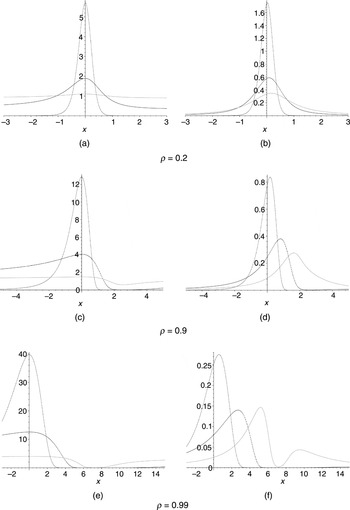
The other term in the density (10)—(1 + w²)⁻¹—is of course symmetric around zero, not −η, so its effect is to shift the mode of the density away from the correct point. In Figure 1 we display both the hypergeometric component of the density (10), that is, the term exp{−½λ}₁F₁(1,½;½λc(w)²) (on the left), and the density itself (on the right), for several values of ρ (ρ = 0.2, 0.9, and 0.99) and, for each of these, for several values of the information quantity

. Thus, when ρ = 0.2, λ = 0.208, 1.05, and 22.2 (Figure 1a), and these values are simply multiplied by 10 and 100, respectively, in Figures 1b and 1c. The functions are displayed as functions of the estimation error e, so the density should ideally be centered at, and concentrated near, zero.

Hypergeometric component and density of e for various values of ρ and the information parameter .

As Figure 1 illustrates, the parameter

determines which of the two turning points dominates the behavior of the hypergeometric component and hence the degree to which the density is concentrated near zero. For small values of

the hypergeometric component of the density is quite flat, and in this case the position and shape of the density are determined almost entirely by those of the function (1 + w²)⁻¹, whose mode (as a function of e) is at e = η (not zero). As

increases the hypergeometric component has more impact, pulling the mode toward the correct point (zero) and increasing the concentration near the mode. As the figures show, for small to moderate values of

, and values of ρ near 1, the density can certainly be bimodal.

2.4. The Direction Estimator

As noted in the Introduction, in two dimensions to declare interest in the ratio of the coordinates of an unknown point (α) is to declare interest in the direction of that point from the origin: the coordinate ratio is constant along lines through the origin. Thus, in the model (1) and (2), interest in β is equivalent to interest in the direction of the vector α in (3). But there are a variety of ways to parameterize direction: by the ratio of coordinates, by points on the circumference of the unit circle (or an ellipse), by the angle the line makes with one axis (i.e., its polar coordinate), and so on. These parameterizations are equivalent, so (at least locally) there are 1–1 functions relating the parameters that define them, and the MLEs for those parameters are automatically related to each other by those same functions.

Thus, for maximum likelihood, it is irrelevant which parameterization is used, but that is not necessarily so for other estimation methods. I argued in Hillier (1990) that the properties of the TSLS estimator (for instance) are distorted by the fact that it is not normalization invariant. In the present (highly simplified) setting the two methods are identical, so that problem does not arise. Nevertheless, the other point made in Hillier (1990)—that the exact properties of estimators are easier to interpret with one parameterization than another—certainly does apply. Indeed, this is no accident: the differential-geometric representation of the density of a statistic explained in Hillier and Armstrong (1999) makes it clear that the density of a given function of some random variables depends crucially on the geometric properties of the manifold (statistic = constant) but not on how that manifold is parameterized. That is, the induced properties of the statistic (its density) will reflect its intrinsic geometric structure but not the manner in which that structure is realized.

So, we can expect to see the “direction” quality of the estimator for β manifest in the distribution of b or, less directly, of w. And indeed it is: the term c(w)² in equation (12) is in fact cos²(ψ), where ψ is the angle between the vectors

which are both points on the unit circle (h′h = φ′φ = 1), so cos(ψ) = h′φ. (Strictly, both h and φ lie on the unit semicircle with positive first coordinate—which is all that is needed to determine β—but it is convenient to think of h as being distributed on the whole circumference of the unit circle by defining pdf (−h) = pdf (h), at the same time identifying −φ with φ.) The random vector h is the “estimator” for φ induced by w, and we may transform w → h as explained in Phillips (1985) and Hillier (1990, Sec. 3). The term (1 + w²)⁻¹ in pdf (w)—the term that in a sense distorts the properties of b—is the Jacobian of the inverse transformation h → w; it arises entirely because of the particular parameterization chosen for the circle.

With this change of attitude (10) becomes the much nicer result

where the density is evaluated with respect to the invariant measure on the unit circle (for details, see Muirhead, 1982, Ch. 2). The properties of h as an estimator of φ are nice: provided λ ≠ 0, pdf (h) is symmetric about the true points ±φ, with modes at ±φ. The concentration of the density of h about these modes—however that is measured—depends only on λ. Thus we have the following result.

PROPOSITION 4. For the direction estimator h, η is a pure location parameter, in the sense that the modes of the density occur at the correct points ±φ, which are determined entirely by η, and λ is a pure concentration parameter.

Remark 6. Equation (14) is easily derived directly from the density of

. First set

, with L as defined in equation (23), which follows, and note that

. Then transform

, with

(the Jacobian is ½), taking account of the sign convention discussed previously. Integration over q > 0 then yields equation (14). The points h indicate the direction of

by projecting onto the unit circle or equivalently that of

by projecting onto the ellipse

.

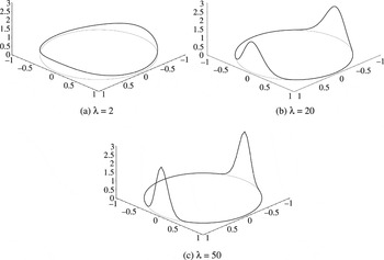
In the totally unidentified case when λ = 0, h is uniformly distributed on the circle, reflecting the fact that h contains no information about φ, as is clearly correct (for more discussion of this, see Hillier, 1990). Figure 2 displays the density of h—supported on the unit circle—for several values of λ. For very small values of λ the density is almost uniform, whereas for large values of λ it is very sharply peaked at its modes ±φ.

Densities of the direction estimator.

Remark 7. In the model (3) parameterized by (α,Ω), the Fisher information matrix is block diagonal with (α,α) block s_ZZΩ⁻¹. When the model is parameterized by (β,γ,Σ), as suggested by (1) and (2), the (partial) information on β is i_ββ = s_ZZγ²/σ_u². When parameterized by first transforming α to α = L′α and then expressing α in polar coordinates (δ,θ) (α′ = (δ sin(θ)),δ cos(θ)), with θ the angle between α and the horizontal axis, the partial information on θ is i_θθ = s_ZZα′Ω⁻¹α = λ. It is clear from (14) that, however the points on the circle are parameterized (i.e., whatever statistic is used to indicate the direction of h), the induced density of the corresponding statistic will depend fundamentally on the information about the direction of α, λ = i_θθ.

3.1. TSLS

Defining e, w, and η as before, the conditional density of e given g ≠ 0 is

and g ∼ N(γ,I_k), where γ = (Z′Z)^1/2γ/σ_v. Hence,

and so

These are the exact analogues of the previous results for the case k = 1. As before, the conditional density of w given g is unimodal. When γ = 0 it is clear from (20) that pdf (w) ∝ (1 + w²)^−(k+1)/2 and is therefore concentrated near the origin (the wrong point), the more so the larger is k.

When γ ≠ 0, integrating out g in (20) is slightly more complicated, but there is a device that simplifies the problem greatly and that, because it does not seem to be widely known, is worth discussing—variations of it are often extremely useful.

The key observation is that the integral in (20), regarded as a function of γ, is invariant under two types of transformation on γ. First, it is invariant under γ → −γ (because, on making this change, we can replace g by −g, leaving the integral unchanged). This means that the term exp{g′γ(1 − ηw)} can be replaced by its average over the two possible signs for γ:

(exactly as in the case k = 1). The final two terms in the integral (20) can therefore be replaced by the double series

But now, by a more general version of the same argument, the resulting integral is also invariant under the transformations γ → Hγ, with H ∈ O(k), the group of k × k orthogonal matrices. This is because, on replacing γ by Hγ, we can then transform g → H′g (a transformation with unit Jacobian), leaving the integral exactly as it was. One implication of this is that the integral (and hence the density) depends on γ only through γ′γ, a maximal invariant under this group of transformations. But it also implies that we can replace γ by Hγ, regard H as a random matrix uniformly distributed on O(k), and integrate over O(k) before integrating out g, and this makes the evaluation of the integral much easier.

The integral over O(k) in this process is of the form ∫_O(k)(g′Hγ)^2r(dH), where (dH) denotes the uniform distribution on O(k). This is the coefficient of t^2r/(2r)! in the expansion of the generating function

(This is a well-known integral—a much more general version of it is given as Theorem 7.4.1 in Muirhead, 1982.) Thus,

These two steps therefore reduce the integrand in equation (20) to a function that depends on g only through q = g′g, and the integral can now be completed by elementary methods (it is essentially a standard Laplace transform), yielding the known (cf. Phillips, 1983, eqn. (3.45)) formula:

where

Note that this can again be expressed in the form

. We may therefore state the following proposition.

PROPOSITION 5. In the overidentified case, the leading term (1 + w²)^−(k+1)/2 in the density of the TSLS estimator is no longer simply the Jacobian of the transformation h → w. The hypergeometric component,

although more complicated, is, as before, a monotonic function of c(w)², and, as before, the location of its turning points is determined entirely by η. Otherwise, the parameters (λ,η) play the same roles as before. The sample size affects the density of the TSLS estimator only through the matrix Z′Z that appears in the definition of λ.

Remark 8.

(i) For the OLS estimator b₀ = (x′x)⁻¹x′y, it is easy to see from (4) that the conditional distribution of the standardized estimator

, given x, has exactly the form (18) with g replaced by the T × 1 vector

, which is N(Zγ/σ_v,I_T) (so that γ is replaced by Zγ/σ_v). Because γ′γ = γ′Z′Zγ/σ_v², it follows that the density of w₀ = e₀ − η has exactly the form (22) with k replaced by the sample size T. This result is well known (cf. Phillips, 1983), but its implications are perhaps not as widely appreciated as they might be. However, for a recent discussion see Kiviet and Niemczyk (2005).

(ii) It is clear again that the density of the TSLS estimator depends on the sample size only through Z′Z. And, from point (i), it follows that the properties of the TSLS estimator as k → ∞ will mimic those of the OLS estimator as T → ∞ if λ remains bounded as T → ∞, as it does under so-called weak-instrument asymptotics. This agrees with recent work on “many weak-instrument asymptotics” by Chao and Swanson (2005, 2006), who show that the TSLS bias converges to that of the OLS estimator as T and k go to infinity (while k/T remains bounded) under weak-instrument asymptotics. See also Phillips (2006) and Newey (2004).

The presence of the term (1 + w²)^−(k+1)/2—which becomes much more concentrated near the origin (the wrong point) as k increases—severely distorts the properties of the TSLS estimator when k is large. We shall see shortly that this effect is not present for the LIML estimator, which helps to explain its apparent superiority over TSLS. Notice too that, if λ = 0, only this term remains, so the density of e becomes concentrated near η, the probability limit of the scaled OLS estimation error when λ = 0. These observations again accord with related work on many-instrument asymptotics for the TSLS and LIML estimators (e.g., Morimune, 1983; Chao and Swanson, 2005, 2006; Newey, 2004), which shows that the LIML estimator is much better centered than the TSLS estimator, and also with important recent results of Chamberlain (2005), which provide a decision-theoretic analysis of this model.

3.2. LIML

The LIML estimator for β maximizes the familiar ratio

Let

so that L′ΩL = I₂. Then define

, a 2 × 2 central Wishart matrix with m = T − k degrees of freedom and covariance matrix

. Finally, put R = (a,g)′(a,g). The supremum of r(β) is the largest root of the equation det[S − fR] = 0, and the LIML estimator for β is defined in terms of the corresponding characteristic vector.

Exact distribution theory for the LIML estimator is, even in the present simplified setup, much more complex than that for the IV (TSLS) estimator. Phillips (1984, 1985) pioneered the theory, but for present purposes it is more convenient to work from Hillier (1987, eqn. (29)), where I obtained the conditional density of (w,f) given R, where w is now the LIML estimator standardized as before and f is the largest root of det[S − fR] = 0. In our present notation, that result yields, after transforming to h, the conditional result

where c_m = [2^m+1Γ((m + 3)/2)Γ(m/2)Γ(½)]⁻¹.

Remark 9. The matrix (a,g) here is a standardized version of the OLS estimator for the complete reduced form coefficient matrix (π,γ) in (16), unconstrained by the requirement that π = γβ. The matrix R (a maximal invariant under the group of transformations (a,g) → H(a,g), H ∈ O(k)) is a natural candidate for testing the general identification condition rank(π,γ) = 1. The conditioning in (24) is thus a generalized version of the conditioning pdf (w|g) used earlier.

Notice that pdf (h|R) depends directly on the sample size (through m) but is parameter free. Thus, the parameters enter the unconditional distribution only through the density of R, and this depends only on k and λ (see equation (A.3) in the Appendix). The marginal density of h is evidently

By some elementary manipulations this expression may be reduced to a form (equation (A.4) in the Appendix) from which the following proposition readily follows.

PROPOSITION 6. For the LIML estimator all of the properties of direction estimator h given in Proposition 4 for the case k = 1 continue to hold in the overidentified case. Transforming to w introduces only the Jacobian term (1 + w²)⁻¹. The density depends on the sample size both directly through m = T − k and indirectly through λ.

Although the formula for the density is considerably more complicated, qualitatively the properties of the LIML estimator in the overidentified case are very similar to those discussed earlier for the case k = 1.