1 Introduction
The study of a localized release of a buoyant fluid within a body of ambient fluid confined vertically (Jirka & Harleman Reference Jirka and Harleman1979) and laterally (Barnett Reference Barnett1993) is of major interest in industrial and environmental flows (Hunt Reference Hunt1991). We investigate the dynamics of a release of buoyant fluid discharged within a tunnel (Barnett Reference Barnett1993) and subjected to a forced mechanical ventilation that drives a bulk horizontal flow, whose velocity is denoted
 $V$
. The tunnel considered is straight and horizontal, and the release is from a source at ground level. A peculiar aspect of these flows (figure 1) is the appearance of a back-layer of buoyant fluid (Salizzoni et al.
Reference Salizzoni, Creyssels, Jiang, Mos, Mehaddi and Vauquelin2018), which forms after impingement of the release with the confining surface (in this application, the tunnel ceiling), and whose front, driven by a horizontal pressure gradient, can propagate against the opposing ventilation depending on its magnitude. Our focus is on the control of the propagation of this buoyant front by means of the forced tunnel ventilation. This issue is directly linked to industrial and transportation safety problems related to the dispersion of harmful gases in confined spaces. Examples include back-layering due to the leakage of high pressure natural gas from pipelines, the accidental releases of hydrogen or hydrogen sulphide, and the propagation of smoke from fires in confined underground spaces (Hunt Reference Hunt1991) and in road and rail tunnels (Grant, Jagger & Lea Reference Grant, Jagger and Lea1998). A solution to this problem is necessary in order to assess the safety of twin-bore road tunnels, where the minimum ventilation velocity
 $V_{c}$
which blows all the smoke downstream, allowing the users to evacuate by the entrance, is usually referred to as the ‘critical velocity’ (Grant et al.
Reference Grant, Jagger and Lea1998).
These practical implications for safety are therefore related to a fundamental problem, namely that of determining the magnitude of the critical velocity of ventilation depending upon the tunnel setting and the geometrical and dynamical conditions at the emission source. Although there is a considerable scatter in the experimental data reported in the ‘tunnel fires’ literature (Jiang et al.
Reference Jiang, Creyssels, Mos and Salizzoni2018), it is usually stated that the critical velocity grows with the cube root of the heat release rate (Thomas Reference Thomas1968). For increasing heat release rate, the dependence of the critical velocity is progressively weakened until reaching, what is regarded as, an asymptotic regime in which the critical velocity appears to be independent of the heat release rate (Oka & Atkinson Reference Oka and Atkinson1995; Grant et al.
Reference Grant, Jagger and Lea1998; Wu & Bakar Reference Wu and Bakar2000; Vauquelin Reference Vauquelin2008). The reason for this behaviour can be attributed to different dynamical aspects whose relative influence on
 $V_{c}$
are not fully understood (Le Clanche et al.
Reference Le Clanche, Salizzoni, Creyssels, Mehaddi, Candelier and Vauquelin2014). To bridge this gap in understanding we develop new theoretical considerations (§ 2) combining them with complementary experimental tests (§ 3). The comparison between the resulting predictions and experimental data finally allows us to identify the role of the key control parameters in the different flow regimes that have been identified herein, regimes that depend on the conditions imposed at the source and on the tunnel geometry.
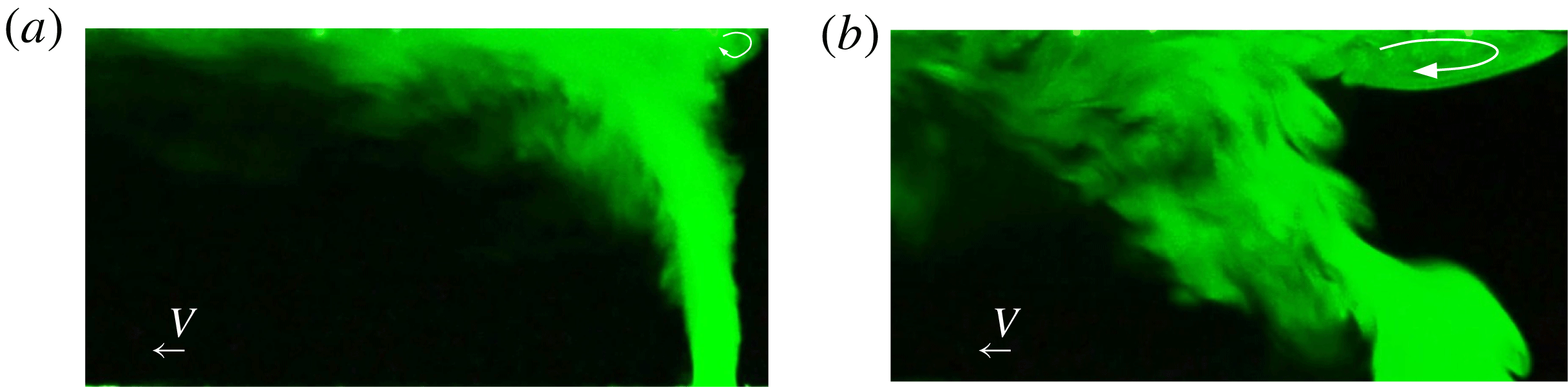
Visualisations of the flow induced by a buoyant emission at ground level subjected to a longitudinal critical ventilation velocity (from right to left): (a) forced release
 $\unicode[STIX]{x1D6E4}_{i}<1$
(with
 $(V_{c}/w_{i})=0.07$
), (b) lazy release
 $\unicode[STIX]{x1D6E4}_{i}>1$
(with
 $(V_{c}/w_{i})=0.30$
).

2 Theory
To begin we consider a horizontal, infinitely long tunnel of height
 $H$
and width
 $W$
(
 ${\sim}H$
) within which a point source of ‘pure’ buoyancy (Morton, Taylor & Turner Reference Morton, Taylor and Turner1956), that gives rise to a turbulent plume, is located centrally on the tunnel floor. Assuming negligible diffusive effects, and in the limit of the Boussinesq approximation, the scaling law for the critical velocity
 $V_{c}$
as a function of the governing parameters, i.e. the buoyancy flux of the source
 $B_{i}$
and a characteristic length, can be derived from dimensional arguments as
 $$\begin{eqnarray}V_{c}=\,f(B_{i},H)\rightarrow V_{c}\propto \left(\frac{B_{i}}{H}\right)^{1/3}.\end{eqnarray}$$
This scaling is suitable for sources whose physical dimensions are much smaller than the tunnel dimensions (
 $H$
and
 $W$
) and for density differences between the buoyant emission and the ambient fluid that are small relative to the ambient. Should these conditions not hold, dimensional considerations have to take into account the characteristic length scale of the source
 $b_{i}$
, the velocity
 $w_{i}$
and density
 $\unicode[STIX]{x1D70C}_{i}$
of the emission, as well as the density of the ambient fluid
 $\unicode[STIX]{x1D70C}_{0}$
and the tunnel dimensions. Retaining the assumption of negligible diffusive effects, the critical velocity can then be expressed as a function of seven dimensional quantities, namely
 $$\begin{eqnarray}V_{c}=f(w_{i},\unicode[STIX]{x1D70C}_{i},\unicode[STIX]{x1D70C}_{0},g,b_{i},W,H),\end{eqnarray}$$
where
 $g$
is the gravitational acceleration. The dimensionless critical velocity is now a function of four dimensionless groups
 $$\begin{eqnarray}\frac{V_{c}}{w_{i}}=f\left(\frac{\unicode[STIX]{x1D702}_{i}gb_{i}}{w_{i}^{2}},\frac{\unicode[STIX]{x1D70C}_{i}}{\unicode[STIX]{x1D70C}_{0}},\frac{b_{i}}{H},\frac{W}{H}\right),\end{eqnarray}$$
with
 $\unicode[STIX]{x1D702}_{i}=(\unicode[STIX]{x1D70C}_{0}-\unicode[STIX]{x1D70C}_{i}/\unicode[STIX]{x1D70C}_{0})$
. The first dimensionless group in (2.3) is usually rescaled as
 $\unicode[STIX]{x1D6E4}_{i}=(5/8\unicode[STIX]{x1D6FC}_{p})(\unicode[STIX]{x1D702}_{i}gb_{i}/w_{i}^{2})$
and referred to as a source Richardson number for the plume where
 $\unicode[STIX]{x1D6FC}_{p}=0.12$
is a reference value (Carazzo, Kaminski & Tait Reference Carazzo, Kaminski and Tait2006) for the ‘top-hat’ entrainment coefficient for a pure plume (Morton et al.
Reference Morton, Taylor and Turner1956). This Richardson number allows for a classification of buoyant releases depending on its value relative to unity: in momentum-dominated forced plumes
 $\unicode[STIX]{x1D6E4}_{i}<1$
; in buoyancy-momentum balanced pure plumes
 $\unicode[STIX]{x1D6E4}_{i}=1$
; and for buoyancy-dominated lazy plumes
 $\unicode[STIX]{x1D6E4}_{i}>1$
(Hunt & Kaye Reference Hunt and Kaye2005).
2.1 Theoretical model
To develop a model that allows us to assess the explicit dependence of the dimensionless critical velocity on the control parameters, equation (2.3), we first appeal to flow visualisations showing the morphology of releases that issue from a circular source placed in the centre of the tunnel (details on experimental set-up and techniques are provided in the next section). The flow visualisations show, in figure 1, the behaviour of a bent-over plume rising to the ceiling. As the plume rises and mixes with the ambient fluid, it is progressively displaced downstream with increasing tunnel ventilation velocity
 $V$
.
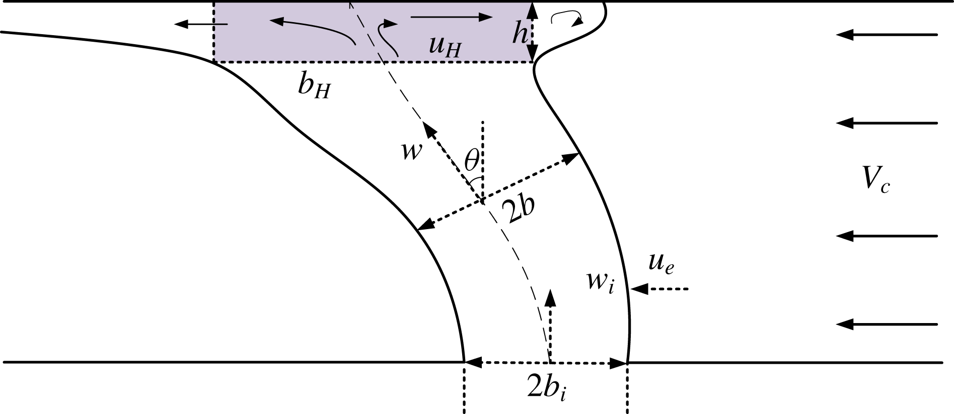
Sketch of a bent-over plume formed from a ground-level circular source in a ventilated tunnel and of the impingement region (in grey) at the tunnel ceiling.

Based on these preliminary observations, the situation considered is illustrated in figure 2, which shows, in schematic form, the evolution of the plume as deflected by the ventilation flow. We represent the buoyant fluid release from the circular source as a ‘top-hat’ plume, following the well-established approach of Morton et al. (Reference Morton, Taylor and Turner1956) and modified by Hoult, Fay & Forney (Reference Hoult, Fay and Forney1969) for plumes in a cross-flow. A mathematical description of the trajectory of the plume can be given in a plume-centred coordinate system (
 $\unicode[STIX]{x1D709}$
denotes the curvilinear abscissa along the plume centre line and
 $\unicode[STIX]{x1D703}$
the inclination of the plume centre line to the vertical axis
 $y$
). The conservation equations for mass, momentum and density deficit can be written as (Hoult et al.
Reference Hoult, Fay and Forney1969; Hewett, Fay & Hoult Reference Hewett, Fay and Hoult1971)
 $$\begin{eqnarray}\displaystyle & \displaystyle \frac{\text{d}}{\text{d}\unicode[STIX]{x1D709}}(\unicode[STIX]{x1D70C}wb^{2})=2\unicode[STIX]{x1D70C}_{0}u_{e}b, & \displaystyle\end{eqnarray}$$
 $$\begin{eqnarray}\displaystyle & \displaystyle \frac{\text{d}}{\text{d}\unicode[STIX]{x1D709}}(\unicode[STIX]{x1D70C}w^{2}b^{2})=(\unicode[STIX]{x1D70C}_{0}-\unicode[STIX]{x1D70C})gb^{2}\cos \unicode[STIX]{x1D703}+2\unicode[STIX]{x1D70C}_{0}Vu_{e}b\sin \unicode[STIX]{x1D703}, & \displaystyle\end{eqnarray}$$
 $$\begin{eqnarray}\displaystyle & \displaystyle \unicode[STIX]{x1D70C}w^{2}b^{2}\frac{\text{d}\unicode[STIX]{x1D703}}{\text{d}\unicode[STIX]{x1D709}}=-(\unicode[STIX]{x1D70C}_{0}-\unicode[STIX]{x1D70C})gb^{2}\sin \unicode[STIX]{x1D703}+2\unicode[STIX]{x1D70C}_{0}Vu_{e}b\cos \unicode[STIX]{x1D703}+{\mathcal{C}}_{D}\unicode[STIX]{x1D70C}_{0}V^{2}b(\cos \unicode[STIX]{x1D703})^{2}, & \displaystyle\end{eqnarray}$$
 $$\begin{eqnarray}\displaystyle & \displaystyle \frac{\text{d}}{\text{d}\unicode[STIX]{x1D709}}[(\unicode[STIX]{x1D70C}_{0}-\unicode[STIX]{x1D70C})wb^{2}]=0, & \displaystyle\end{eqnarray}$$
 $\unicode[STIX]{x1D70C}$
,
 $u$
and
 $w$
are the (time averaged) density, longitudinal velocity and vertical velocity of the plume, respectively,
 $u_{e}$
is the entrainment velocity at the perimeter of the plume and
 ${\mathcal{C}}_{D}$
is a drag coefficient for the force exerted by the plume on the longitudinal ventilation flow. For releases in a cross-wind environment, the entrainment velocity is usually modelled (Hewett et al.
Reference Hewett, Fay and Hoult1971; Devenish et al.
Reference Devenish, Rooney, Webster and Thomson2010; Marro et al.
Reference Marro, Salizzoni, Cierco, Korsakissok, Danzi and Soulhac2014; Woodhouse et al.
Reference Woodhouse, Hogg, Phillips and Sparks2013) as the sum of two contributions, related to the differences of the velocity components tangential and perpendicular to the plume axis
 $$\begin{eqnarray}u_{e}=\unicode[STIX]{x1D6FC}|u-V\sin \unicode[STIX]{x1D703}|+\unicode[STIX]{x1D6FD}|V\cos \unicode[STIX]{x1D703}|.\end{eqnarray}$$
The quantities
 $\unicode[STIX]{x1D6FC}$
,
 $\unicode[STIX]{x1D6FD}$
and
 ${\mathcal{C}}_{D}$
are quantities that have to be determined experimentally and that, in principle, depend on the form of the release and its dynamical conditions, i.e. on
 $\unicode[STIX]{x1D6E4}_{i}$
and the density ratio
 $\unicode[STIX]{x1D70C}/\unicode[STIX]{x1D70C}_{0}$
(Aubry et al.
Reference Aubry, Jelline, Carazzo, Gallo, Hatcher and Dunning2017). In the literature, their values vary considerably: Hoult et al. (Reference Hoult, Fay and Forney1969) used
 $\unicode[STIX]{x1D6FC}=0.15$
,
 $\unicode[STIX]{x1D6FD}=0.9$
and
 ${\mathcal{C}}_{D}=0$
; Suzuki & Koyaguchi (Reference Suzuki and Koyaguchi2015) estimated
 $\unicode[STIX]{x1D6FC}$
in the range 0.05–0.06,
 $\unicode[STIX]{x1D6FD}$
in the range 0.1–0.3 with
 ${\mathcal{C}}_{D}=0$
; and Robins et al. (Reference Robins, Apsley, Carruthers, McHugh and Dyster2009) adopted
 $\unicode[STIX]{x1D6FC}=0.06$
,
 $\unicode[STIX]{x1D6FD}=0.5$
and
 $C_{D}=0.21$
. An overview of the literature reveals, however, that the range of values for the entrainment coefficient
 $\unicode[STIX]{x1D6FC}$
is significantly narrower than that for the values for
 $\unicode[STIX]{x1D6FD}$
and
 ${\mathcal{C}}_{D}$
.
The model (2.4a
)
 $-$
(2.4d
) does not take into account pressure gradients and turbulent fluxes, whose roles are not necessarily negligible when considering the flow developing within a few source radii (Craske & van Reeuwijk Reference Craske and van Reeuwijk2015; Ezzamel, Salizzoni & Hunt Reference Ezzamel, Salizzoni and Hunt2015), i.e. we implicitly assume
 $b_{i}\ll H$
. Furthermore, the model as conceived is clearly unable to simulate any effect of the flow induced by the presence of side walls and, therefore, the influence of the aspect ratio
 $H/W$
. Numerical solution of (2.4a
)
 $-$
(2.4d
), subject to appropriate boundary conditions at the source, would allow us to compute the plume trajectory, its impingement point and determine the plume conditions (radius, velocity and density) at impingement under the aforementioned assumptions.
In order to achieve approximate analytical solutions, revealing a general dependence of the dimensionless critical velocity on the control parameters, we can however further simplify the formulation of the model based on the following considerations. In the tunnel safety literature (Grant et al.
Reference Grant, Jagger and Lea1998) the critical velocity is generally defined as that preventing the back-layer flow from moving upstream of the source or, alternatively, as the minimum ventilation velocity
 $V_{c}$
that prevents the formation of the back-layer flow (figure 1). By adopting here the latter definition, the critical velocity condition does not depend on the impingement point of the plume at the ceiling. Its evaluation therefore, to a first approximation, does not require one to evaluate the trajectory of the plume centre line. If we further assume that the plume bends only slightly from the vertical direction (i.e.
 $\unicode[STIX]{x1D703}\rightarrow 0$
), which implies that the ventilation velocity is smaller than the plume vertical velocity (i.e.
 $V\ll w$
) we can: (i) avoid taking into account the role of the horizontal momentum balance (2.4c
) and (ii) simplify the entrainment relation (2.5) to
 $u_{e}=\unicode[STIX]{x1D6FC}w$
. Accordingly, equations (2.4a
), (2.4b
) and (2.4d
) reduce to
 $$\begin{eqnarray}\displaystyle & \displaystyle \frac{\text{d}}{\text{d}y}(\unicode[STIX]{x1D70C}wb^{2})=2\unicode[STIX]{x1D70C}_{0}\unicode[STIX]{x1D6FC}wb, & \displaystyle\end{eqnarray}$$
 $$\begin{eqnarray}\displaystyle & \displaystyle \frac{\text{d}}{\text{d}y}(\unicode[STIX]{x1D70C}w^{2}b^{2})=(\unicode[STIX]{x1D70C}_{0}-\unicode[STIX]{x1D70C})gb^{2}, & \displaystyle\end{eqnarray}$$
 $$\begin{eqnarray}\displaystyle & \displaystyle \frac{\text{d}}{\text{d}y}[(\unicode[STIX]{x1D70C}_{0}-\unicode[STIX]{x1D70C})wb^{2}]=0, & \displaystyle\end{eqnarray}$$
 $b(0)=b_{i}$
,
 $w(0)=w_{i}$
,
 $\unicode[STIX]{x1D70C}(0)=\unicode[STIX]{x1D70C}_{i}$
. Broadly speaking, we expect these simplifying assumptions to hold in the case of forced releases, i.e. those that are momentum dominated, issuing from sources of small diameter (relative to the tunnel width and height) and that bend only slightly when exposed to the critical ventilation velocity (see figure 2). By contrast, the reliability of these assumptions is questionable for lazy releases, i.e. those of larger diameters and with lower velocities at the source.
2.2 Critical velocity condition
In order to prevent the formation of the back-layer flow, the ventilation has to impose a force which balances that of the opposing lateral flow, or current, induced by the impingement of the buoyant release at the tunnel ceiling (figure 2). A simplified model describing the impingement process is provided by Kaye & Hunt (Reference Kaye and Hunt2007), based on the conservation equations for mass and momentum for the turning region
 $$\begin{eqnarray}\left.\begin{array}{@{}c@{}}{b_{H}}^{2}\unicode[STIX]{x1D70C}_{H}w_{H}=(2b_{H})h\unicode[STIX]{x1D70C}_{H}U,\\ {b_{H}}^{2}\unicode[STIX]{x1D70C}_{H}{w_{H}}^{2}=\unicode[STIX]{x1D6FE}(2b_{H})h\unicode[STIX]{x1D70C}_{H}U^{2},\end{array}\right\}\end{eqnarray}$$
where throughout the subscript
 $(\cdot )_{H}$
signifies quantities evaluated at the ceiling and
 $\unicode[STIX]{x1D6FE}$
(
 ${\leqslant}1$
) is a head-loss coefficient (Kaye & Hunt Reference Kaye and Hunt2007), that, in principle, is a function of the dynamical condition of the buoyant plume at impingement, i.e.
 $\unicode[STIX]{x1D6FE}=\unicode[STIX]{x1D6FE}(H,\unicode[STIX]{x1D6E4}_{i},b_{i})$
. In (2.7),
 $h$
denotes the depth of the current at the critical condition and
 $U\equiv |u_{H}|$
is the plume’s lateral velocity after impingement (figure 2). Since the layer formed by the buoyant fluid discharging from the plume is not expected to be vanishingly thin (Manins Reference Manins1979), it could be argued that the flow variables in (2.7) should be evaluated at a height lower than
 $H$
. Adopting this procedure would however introduce further complexity to the model without adding any considerable further insight to our investigation, whose primary aim is the identification of the main tendencies of the dimensionless critical velocity on the control parameters (2.3).
The critical ventilation condition can be modelled by assuming that, immediately after impingement, the momentum flux imposed by the ventilation flow balances the longitudinal momentum flux and the pressure force of the buoyant flow at the ceiling
 $$\begin{eqnarray}\unicode[STIX]{x1D70C}_{0}{V_{c}}^{2}=\unicode[STIX]{x1D711}[\unicode[STIX]{x1D70C}_{H}U^{2}+{\textstyle \frac{1}{2}}(\unicode[STIX]{x1D70C}_{0}-\unicode[STIX]{x1D70C}_{H})gh],\end{eqnarray}$$
where the dimensionless quantity
 $\unicode[STIX]{x1D711}$
is a constant that we expect to be of order one and that has to be determined experimentally. It is worth noting that the system (2.7) actually refers to an impinging plume in the absence of ventilation. The resulting model (2.8) has therefore to be considered as an approximation of the critical ventilation condition, resulting from a considerable simplification of the flow conditions occurring in the tunnel.
By means of the coupled equations (2.7), one can express the flow variables as
 $U=w_{H}/\unicode[STIX]{x1D6FE}$
and
 $h=\unicode[STIX]{x1D6FE}b_{H}/2$
, so that (2.8) can be rewritten as
 $$\begin{eqnarray}\unicode[STIX]{x1D70C}_{0}{V_{c}}^{2}=\frac{\unicode[STIX]{x1D711}}{\unicode[STIX]{x1D6FE}^{2}}\unicode[STIX]{x1D70C}_{H}{w_{H}}^{2}\left[1+\left(\frac{4}{5}\right)\frac{\unicode[STIX]{x1D6FC}_{p}\unicode[STIX]{x1D6FE}^{3}}{2}\frac{\unicode[STIX]{x1D70C}_{0}}{\unicode[STIX]{x1D70C}_{H}}\unicode[STIX]{x1D6E4}_{H}\right],\end{eqnarray}$$
where
 $\unicode[STIX]{x1D6E4}_{H}=(5/8\unicode[STIX]{x1D6FC}_{p})(\unicode[STIX]{x1D702}_{H}gb_{H}/w_{H}^{2})$
is the plume Richardson number at impingement (i.e. evaluated at
 $y=H$
). Experimental estimates of the head losses in impinging plumes and jets indicate that
 $\unicode[STIX]{x1D6FE}\sim 1$
(Ezzamel Reference Ezzamel2011). We therefore obtain an estimate of the term
 $(\unicode[STIX]{x1D6FC}_{p}\unicode[STIX]{x1D6FE}^{3}/2)\simeq 0.06$
, which implies that the pressure term is negligible compared to the momentum term in the right-hand side of (2.9), both for pure and lazy plumes, for which we expect
 $\unicode[STIX]{x1D6E4}_{H}=1$
and
 $\unicode[STIX]{x1D6E4}_{H}\sim 1$
, respectively (see also discussion in § 2.4), and for forced plumes
 $\unicode[STIX]{x1D6E4}_{H}<1$
. Accordingly (2.9) can be approximated as
 $$\begin{eqnarray}\frac{V_{c}}{w_{i}}=C\left(\frac{\unicode[STIX]{x1D70C}_{H}}{\unicode[STIX]{x1D70C}_{0}}\right)^{1/2}\frac{w_{H}}{w_{i}},\end{eqnarray}$$
where
 $C=\sqrt{\unicode[STIX]{x1D711}/\unicode[STIX]{x1D6FE}^{2}}$
depends on
 $\unicode[STIX]{x1D6E4}_{H}$
, since
 $\unicode[STIX]{x1D6FE}=\unicode[STIX]{x1D6FE}(\unicode[STIX]{x1D6E4}_{H})$
.
The system of equations (2.6a )–(2.6c ) and (2.7) represents a simplified model of the dynamics of the buoyant fluid release, of its interaction with the ventilation flow and of its impingement point at the tunnel ceiling.
Implicit in the model development is that the ventilation velocity is much lower than the plume velocity at impingement, i.e.
 $V\ll w_{H}$
, and that the plume diameter at the ceiling is less than the tunnel width, i.e.
 $$\begin{eqnarray}2\left(b_{i}+\int _{0}^{H}\frac{\text{d}b}{\text{d}y}\,\text{d}y\right)<W.\end{eqnarray}$$
If we consider a general overestimate of the plume radius at the ceiling by assuming a pure-plume growth rate for all
 $y$
, i.e. substituting
 $\text{d}b/\text{d}y=6\unicode[STIX]{x1D6FC}_{p}/5$
, then (2.11) imposes the following restriction on the physical scale of the source
 $$\begin{eqnarray}\frac{b_{i}}{W}<\frac{1}{2}\left(1-\frac{12\unicode[STIX]{x1D6FC}_{p}}{5}\frac{H}{W}\right).\end{eqnarray}$$
Regarding these assumptions and their resulting constraints (to which we will return in § 4), it is worth remembering that adopting such a model is motivated by the aim of capturing the main bulk phenomena governing the dynamics of the flow, rather than providing a detailed description of the flow.
2.3 Analytical solutions
Adopting an entrainment coefficient of the form
 $\unicode[STIX]{x1D6FC}=\unicode[STIX]{x1D6FC}_{p}(\unicode[STIX]{x1D70C}/\unicode[STIX]{x1D70C}_{0})^{1/2}$
(Rooney & Linden Reference Rooney and Linden1996; Woods Reference Woods1997; van den Bremer & Hunt Reference van den Bremer and Hunt2010), an analytical solution of the system (2.6a
)
 $-$
(2.6c
) can be obtained, based on the solution of a freely propagating area source plume in an unstratified atmosphere (Hunt & Kaye Reference Hunt and Kaye2005; Michaux & Vauquelin Reference Michaux and Vauquelin2008; van den Bremer & Hunt Reference van den Bremer and Hunt2010). To that end, we rewrite (2.6a
)
 $-$
(2.6c
) introducing a modified plume radius
 $\widetilde{b}=(\unicode[STIX]{x1D70C}/\unicode[STIX]{x1D70C}_{0})^{1/2}b$
and a modified dimensionless density deficit
 $\widetilde{\unicode[STIX]{x1D702}}=(\unicode[STIX]{x1D70C}_{0}-\unicode[STIX]{x1D70C})/\unicode[STIX]{x1D70C}$
 $$\begin{eqnarray}\displaystyle & \displaystyle \frac{\text{d}}{\text{d}y}(w\widetilde{b}^{2})=2\unicode[STIX]{x1D6FC}_{p}w\widetilde{b}, & \displaystyle\end{eqnarray}$$
 $$\begin{eqnarray}\displaystyle & \displaystyle \frac{\text{d}}{\text{d}y}(w^{2}\widetilde{b}^{2})=\widetilde{\unicode[STIX]{x1D702}}g\widetilde{b}^{2}, & \displaystyle\end{eqnarray}$$
 $$\begin{eqnarray}\displaystyle & \displaystyle \frac{\text{d}}{\text{d}y}(\widetilde{\unicode[STIX]{x1D702}}w\widetilde{b}^{2})=0. & \displaystyle\end{eqnarray}$$
 $-$
(2.13c
) subject to (
 $w=w_{i}$
,
 $\widetilde{b}=\widetilde{b}_{i}$
,
 $\widetilde{\unicode[STIX]{x1D702}}=\widetilde{\unicode[STIX]{x1D702}}_{i}$
) on
 $y=0$
shows that the dimensionless plume velocity, modified radius and density deficit can be expressed as a function of the plume Richardson number only
 $$\begin{eqnarray}\left.\begin{array}{@{}c@{}}\displaystyle \frac{w}{w_{i}}=\left(\frac{\widetilde{\unicode[STIX]{x1D6E4}}_{i}}{\widetilde{\unicode[STIX]{x1D6E4}}}\right)^{1/2}\left(\frac{1-\widetilde{\unicode[STIX]{x1D6E4}}}{1-\widetilde{\unicode[STIX]{x1D6E4}}_{i}}\right)^{1/10},\\ \displaystyle \frac{\widetilde{b}}{\widetilde{b}_{i}}=\left(\frac{\widetilde{\unicode[STIX]{x1D6E4}}}{\widetilde{\unicode[STIX]{x1D6E4}}_{i}}\right)^{1/2}\left(\frac{1-\widetilde{\unicode[STIX]{x1D6E4}}_{i}}{1-\widetilde{\unicode[STIX]{x1D6E4}}}\right)^{3/10},\\ \displaystyle \frac{\widetilde{\unicode[STIX]{x1D702}}}{\widetilde{\unicode[STIX]{x1D702}}_{i}}=\left(\frac{\widetilde{\unicode[STIX]{x1D6E4}}_{i}}{\widetilde{\unicode[STIX]{x1D6E4}}}\right)^{1/2}\left(\frac{1-\widetilde{\unicode[STIX]{x1D6E4}}}{1-\widetilde{\unicode[STIX]{x1D6E4}}_{i}}\right)^{1/2},\end{array}\right\}\end{eqnarray}$$
where
 $\widetilde{\unicode[STIX]{x1D6E4}}=(5g/8\unicode[STIX]{x1D6FC}_{p})(\widetilde{\unicode[STIX]{x1D702}}\,\widetilde{b}/w^{2})$
is a modified local plume Richardson number which varies with height according to
 $$\begin{eqnarray}{\mathcal{G}}(\widetilde{\unicode[STIX]{x1D6E4}})={\mathcal{G}}(\widetilde{\unicode[STIX]{x1D6E4}}_{i})+\frac{y}{\unicode[STIX]{x1D6EC}_{i}},\end{eqnarray}$$
with
 $\unicode[STIX]{x1D6EC}_{i}=(\widetilde{b}_{i}/4\unicode[STIX]{x1D6FC}_{p})(|\widetilde{\unicode[STIX]{x1D6E4}}_{i}-1|^{3/10}/\widetilde{\unicode[STIX]{x1D6E4}}_{i}^{1/2})$
a length (characteristic of that needed to attain a pure plume balance) imposed by the conditions at the source, and the function
 ${\mathcal{G}}$
defined as
 $$\begin{eqnarray}\displaystyle {\mathcal{G}}(X)=\int _{0}^{X}x^{-1/2}(1-x)^{-13/10}\,\text{d}x\quad \text{for}~X<1, & & \displaystyle\end{eqnarray}$$
 $$\begin{eqnarray}\displaystyle {\mathcal{G}}(X)=\int _{X}^{\infty }x^{-1/2}(x-1)^{-13/10}\,\text{d}x\quad \text{for}~X>1. & & \displaystyle\end{eqnarray}$$
 $w_{H}$
and
 $\unicode[STIX]{x1D70C}_{H}$
, given by (2.14) with
 $\widetilde{\unicode[STIX]{x1D6E4}}=\widetilde{\unicode[STIX]{x1D6E4}}_{H}$
, into (2.10)
 $$\begin{eqnarray}\frac{V_{c}}{w_{i}}=C\left(\frac{\widetilde{\unicode[STIX]{x1D6E4}}_{i}}{\widetilde{\unicode[STIX]{x1D6E4}}_{H}}\right)^{1/2}\left(\frac{1-\widetilde{\unicode[STIX]{x1D6E4}}_{H}}{1-\widetilde{\unicode[STIX]{x1D6E4}}_{i}}\right)^{1/10}\left[1+\widetilde{\unicode[STIX]{x1D702}}_{i}\left(\frac{1-\widetilde{\unicode[STIX]{x1D6E4}}_{H}}{1-\widetilde{\unicode[STIX]{x1D6E4}}_{i}}\right)^{1/2}\left(\frac{\widetilde{\unicode[STIX]{x1D6E4}}_{i}}{\widetilde{\unicode[STIX]{x1D6E4}}_{H}}\right)^{1/2}\right]^{-1/2},\end{eqnarray}$$
with
 $C=C(\widetilde{\unicode[STIX]{x1D6E4}}_{H})$
.
2.4 Asymptotic behaviours
It is instructive to investigate the solutions of (2.17) in the limits of highly forced (
 $\unicode[STIX]{x1D6E4}_{i}\rightarrow 0$
) and highly lazy (
 $\unicode[STIX]{x1D6E4}_{i}\rightarrow \infty$
) releases. In doing so we refer to the main findings of plume theory (Hunt & Kaye Reference Hunt and Kaye2005; van den Bremer & Hunt Reference van den Bremer and Hunt2010), indicating that the lower the value of
 $\unicode[STIX]{x1D6E4}_{i}$
(or
 $\widetilde{\unicode[STIX]{x1D6E4}}_{i}$
), the larger the distance (in units of the modified source length scale) needed to approach the pure plume condition,
 $\unicode[STIX]{x1D6E4}=1$
.
2.4.1 Forced releases
Given the relatively short distance between source and ceiling (relative to the height expected in practice for a tunnel release to change asymptotically to the pure plume balance), we assume here that highly forced emissions, i.e.
 $\widetilde{\unicode[STIX]{x1D6E4}}_{i}\rightarrow 0$
, impinge the ceiling with an identical balance of fluxes, i.e.
 $\widetilde{\unicode[STIX]{x1D6E4}}(y=H)\rightarrow \widetilde{\unicode[STIX]{x1D6E4}}_{i}$
. With this assumption, equation (2.16a
) becomes
 ${\mathcal{G}}(\widetilde{\unicode[STIX]{x1D6E4}})=2\widetilde{\unicode[STIX]{x1D6E4}}^{1/2}$
and, making use of (2.15), we obtain
 $\widetilde{\unicode[STIX]{x1D6E4}}_{H}=(1+2\unicode[STIX]{x1D6FC}_{p}H/\widetilde{b}_{i})^{2}\widetilde{\unicode[STIX]{x1D6E4}}_{i}$
. Thus, for forced plumes, equation (2.17) can be approximated as
 $$\begin{eqnarray}\frac{V_{c}}{w_{i}}=\frac{C_{F}}{1+2\unicode[STIX]{x1D6FC}_{p}H/\widetilde{b}_{i}}\left(1+{\displaystyle \frac{{\displaystyle \frac{\unicode[STIX]{x1D70C}_{0}}{\unicode[STIX]{x1D70C}_{i}}}-1}{1+2\unicode[STIX]{x1D6FC}_{p}H/\widetilde{b}_{i}}}\right)^{-1/2},\end{eqnarray}$$
with
 $C_{F}=C(\widetilde{\unicode[STIX]{x1D6E4}}_{H}\rightarrow 0)$
, a relation that does not imply a dependence on the source Richardson number.
2.4.2 Lazy releases
In comparison to forced plumes (van den Bremer & Hunt Reference van den Bremer and Hunt2010), lazy emissions rapidly approach the condition of a pure plume (
 $\widetilde{\unicode[STIX]{x1D6E4}}\rightarrow 1^{+}$
) as
 $\widetilde{\unicode[STIX]{x1D6E4}}$
decreases quickly with distance from the source. We therefore assume that for
 $\widetilde{\unicode[STIX]{x1D6E4}_{i}}>1$
, the release impinges the ceiling with the condition
 $\widetilde{\unicode[STIX]{x1D6E4}}(y=H)\rightarrow 1$
. With this assumption, equation (2.16b
) becomes
 ${\mathcal{G}}(\widetilde{\unicode[STIX]{x1D6E4}}_{H})=10/3(\widetilde{\unicode[STIX]{x1D6E4}}_{H}-1)^{-3/10}$
whereas
 ${\mathcal{G}}(\widetilde{\unicode[STIX]{x1D6E4}}_{i})=5/4(\widetilde{\unicode[STIX]{x1D6E4}}_{i})^{-4/5}$
when
 $\widetilde{\unicode[STIX]{x1D6E4}}_{i}\gg 1$
. Then, equation (2.15) implies that
 $$\begin{eqnarray}\left(\frac{\widetilde{\unicode[STIX]{x1D6E4}}_{H}-1}{\widetilde{\unicode[STIX]{x1D6E4}}_{i}-1}\right)^{-3/10}=\frac{6\unicode[STIX]{x1D6FC}_{p}}{5}\frac{H}{\widetilde{b}_{i}}\widetilde{\unicode[STIX]{x1D6E4}}_{i}^{1/2}.\end{eqnarray}$$
Noting that
 $\widetilde{b}\widetilde{\unicode[STIX]{x1D6E4}}=b\unicode[STIX]{x1D6E4}$
, equation (2.17) can be used to approximate the critical velocity as
 $$\begin{eqnarray}\frac{V_{c}}{w_{i}}=C_{L}\left(\frac{5}{6\unicode[STIX]{x1D6FC}_{p}}\frac{b_{i}}{H}\unicode[STIX]{x1D6E4}_{i}\right)^{1/3},\end{eqnarray}$$
with
 $C_{L}=C(\unicode[STIX]{x1D6E4}_{H}\rightarrow 1)$
. Finally, expressing
 $\unicode[STIX]{x1D6E4}_{i}$
as a function of the buoyancy flux
 $$\begin{eqnarray}B_{i}=\unicode[STIX]{x03C0}b_{i}^{2}w_{i}g\unicode[STIX]{x1D702}_{i},\end{eqnarray}$$
both
 $w_{i}$
and
 $b_{i}$
vanish in (2.20) leading to
 $$\begin{eqnarray}V_{c}=\widehat{\text{Fr}}_{c}\,\left(\frac{B_{i}}{H}\right)^{1/3}\quad \text{as }\unicode[STIX]{x1D6E4}_{i}\rightarrow \infty .\end{eqnarray}$$
The constant
 $\widehat{\text{Fr}}_{c}=(25/48\unicode[STIX]{x03C0}\unicode[STIX]{x1D6FC}_{p}^{2})^{1/3}C_{L}$
is a critical Froude number (or equivalently, a rescaled dimensionless critical velocity) and is independent both of the tunnel and source geometries. Equation (2.22) expresses that, for highly lazy plumes, the dynamical similarity conditions of the flow are reduced to a single dimensionless parameter. In other words, the governing parameters in (2.2) (for a fixed tunnel geometry) are identical to those of a point source of pure buoyancy as in (2.1), and are fully represented by the source buoyancy flux
 $B_{i}$
(without any need to provide information about radius
 $b_{i}$
and density
 $\unicode[STIX]{x1D70C}_{i}$
). This is a direct consequence of the assumption that, for lazy releases,
 $\widetilde{\unicode[STIX]{x1D6E4}}(y=H)\rightarrow 1$
.
In the following we explore experimentally the dynamics of these buoyant releases by investigating the functional dependence expressed by (2.3), and discuss reasons for the agreement with and discrepancies between the experimental data and our theoretical predictions. Our aim is to extend and complete the analysis presented by Le Clanche et al. (Reference Le Clanche, Salizzoni, Creyssels, Mehaddi, Candelier and Vauquelin2014), that mainly focused on buoyancy-dominated releases, and investigate (2.3) for a wide range of dynamical conditions at the source, spanning from almost pure jets (
 $\unicode[STIX]{x1D6E4}_{i}\ll 1$
) to highly lazy plumes (
 $\unicode[STIX]{x1D6E4}_{i}\gg 1$
). Our focus is mainly on the roles of
 $\unicode[STIX]{x1D6E4}_{i}$
and the density ratio
 $\unicode[STIX]{x1D70C}_{i}/\unicode[STIX]{x1D70C}_{0}$
, the latter being the key dimensionless parameter used to evaluate dynamical effects referred to as ‘non-Boussinesq’ (Ricou & Spalding Reference Ricou and Spalding1961; Rooney & Linden Reference Rooney and Linden1996) whose influence, in the current context, has still not been fully elucidated. The comparison between the experimental data and our theoretical predictions, i.e. solution of (2.17)–(2.22), are then used to assess the reliability of the assumptions on which the model is based and thereby provide further insight regarding the influence of the parameters governing the dynamics of tunnel ventilation flow.
3 Experiments
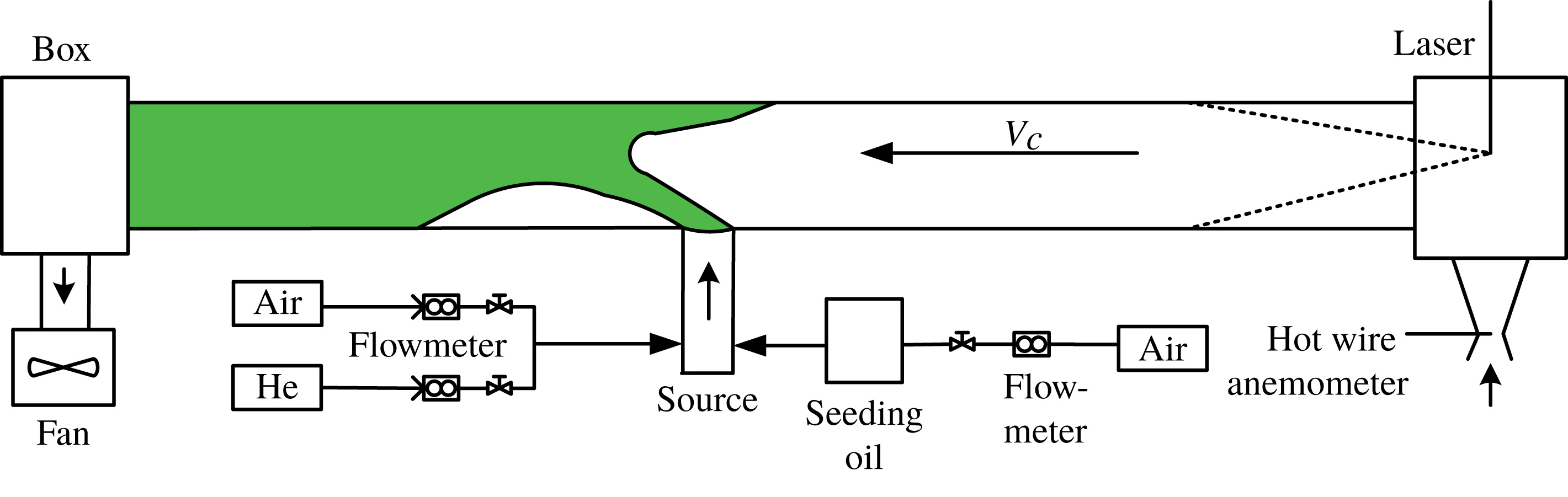
Experiments were performed in a reduced-scale model tunnel (figure 3) of length
 $L=8.9~\text{m}$
, width
 $W=0.36~\text{m}$
, and variable height,
 $H=0.18~\text{m}$
and
 $H=0.36~\text{m}$
. The transparent side walls were made of toughened glass so as to permit visualisation of the flow. The releases of buoyant fluid were mixtures of air and helium (He), whose flow rates were controlled independently and measured by two flowmeters. Experiments were performed with circular sources positioned at the centre of the tunnel. To visualise the flow, the buoyant mixture was seeded with nebulised oil and lit with a laser sheet emitted through a lens installed at the inlet of the tunnel. The mass of oil added to seed the buoyant release was a tiny fraction of the total mass injected at the source (inducing variations of the density of the mixture of order
 $10^{-5}~\text{kg}~\text{m}^{-3}$
). The longitudinal ventilation was imposed by a fan at the downstream end of the tunnel. The flow rate within the tunnel was estimated by means of a hot-wire anemometer placed within a Venturi tube at the inlet, providing a spatially averaged velocity over the tunnel section in the range
 $0.11\leqslant V\leqslant 1.15~\text{m}~\text{s}^{-1}$
.
Schematic of the experimental set-up.

The velocity at the source of the release could be varied within the range
 $0.17\leqslant w_{i}\leqslant 11~\text{m}~\text{s}^{-1}$
, producing a buoyancy flux in the range
 $1\times 10^{-3}\leqslant B_{i}\leqslant 6.3\times 10^{-2}~\text{m}^{4}~\text{s}^{-3}$
as evaluated from (2.21). Experimental results were obtained by varying the values of the three control parameters, i.e.
 $\unicode[STIX]{x1D6E4}_{i}$
,
 $b_{i}/H$
and
 $\unicode[STIX]{x1D70C}_{i}/\unicode[STIX]{x1D70C}_{0}$
.
The parameters spanned the ranges
 $0.004<\unicode[STIX]{x1D6E4}_{i}<24$
,
 $0.25<\unicode[STIX]{x1D70C}_{i}/\unicode[STIX]{x1D70C}_{0}<0.92$
and
 $0.034\leqslant b_{i}/H\leqslant 0.270$
(source diameters measured as
 $2b_{i}=$
0.100, 0.075, 0.050, 0.035, 0.025 m). These releases were characterised by values of the non-Boussinesq length
 $z_{b}=5/3(B_{i}^{2}/20\unicode[STIX]{x1D6FC}_{p}^{4}g^{3})^{1/5}$
(Woods Reference Woods1997), over which density ratio variations are expected to affect the flow dynamics, in the range
 $0.6H<z_{b}<1.6H$
. For the tunnel aspect ratios considered,
 $H/W=1.0$
and
 $0.5$
, equation (2.12) indicates that, to enable meaningful comparison between data and the theory,
 $b_{i}/W$
should not exceed
 $0.38$
and
 $0.44$
, respectively. Across all of the experiments
 $b_{i}/W\leqslant 0.135$
such that (2.12) is satisfied. Moreover, an underlying assumption upon which the model is based is that the plume is long and slender, in particular
 $b_{i}\ll H$
. Whilst this is achieved for some experiments (e.g. with
 $b_{i}/H=0.034$
) it is not achieved for all (e.g. with
 $b_{i}/H=0.270$
).
Results could be produced only for limited combinations of the control parameters within the ranges given. Experimental conditions were constrained by the power of the fan used to produce the longitudinal ventilation, the measurement range of the flowmeters, the availability of helium and by the source Reynolds number. The latter, defined as
 $Re_{i}=2w_{i}b_{i}/\unicode[STIX]{x1D708}$
(
 $\unicode[STIX]{x1D708}$
denoting the kinematic viscosity of the released fluid), had to be kept sufficiently high to avoid viscous effects. To ensure a turbulent release, larger radii had to be adopted for larger
 $\unicode[STIX]{x1D6E4}_{i}$
.
These limitations did not allow us to produce
 $\unicode[STIX]{x1D6E4}_{i}>2$
releases with ‘small’ radii (i.e. for
 $b_{i}/H<0.15$
) or highly-forced (
 $\unicode[STIX]{x1D6E4}_{i}\ll 1$
) non-Boussinesq (
 $\unicode[STIX]{x1D70C}_{i}/\unicode[STIX]{x1D70C}_{0}<0.15$
) releases with ‘large’ radii (i.e. for
 $b_{i}/H>0.3$
). The Reynolds number varied in the range
 $700<Re_{i}<11\,100$
. Note that
 $Re_{i}$
generally decreased with increasing
 $\unicode[STIX]{x1D6E4}_{i}$
, with
 $2500<Re_{i}<11\,000$
for
 $\unicode[STIX]{x1D6E4}_{i}<0.5$
,
 $1000<Re_{i}<6000$
for
 $0.5<\unicode[STIX]{x1D6E4}_{i}<1$
and
 $700<Re_{i}<2000$
for
 $\unicode[STIX]{x1D6E4}_{i}>1$
. All releases exceeded the critical value
 $Re_{i}=Re_{cr}=600$
, indicated by Arya & Lape (Reference Arya and Lape1990) as a threshold ensuring negligible viscous effects on buoyant releases in a cross-flow. Achieving
 $Re_{i}>600$
significantly limited an exploration of the effect of a varying radius at large
 $\unicode[STIX]{x1D6E4}_{i}$
, whereas the constraint on achieving low
 $\unicode[STIX]{x1D6E4}_{i}$
releases was limited primarily by the power of the fan producing the tunnel ventilation.
The experimental evaluation of the critical velocity by means of flow visualisation is straightforward, since it solely requires, once the source conditions of the emission are fixed, an adjustment of the fan power to stop the propagation of the back-layering front immediately after its formation. This flow configuration is characterised by the occurrence of a vortex of buoyant flow at the ceiling, immediately after the impingement point (figure 1). This protocol inevitably involves a number of experimental uncertainties in determining the position of the front, which actually oscillates around its time-averaged position owing to turbulent fluctuations. To estimate these uncertainties we performed 20 independent iterations of the same experiment, for a reduced number of experimental conditions. For each of these conditions, the uncertainty was then quantified as half of the difference between the minimum and maximum value of
 $V_{c}$
. This never exceeded
 $\pm 10\,\%$
, which was thereafter taken to be the reference value of the experimental uncertainty.
To analyse the dependence of
 $V_{c}/w_{i}$
on each of the key dimensionless groups given in (2.3) we performed a different series of experiments. In each series, we conveniently changed the values of the control parameters at the source, i.e.
 $w_{i}$
,
 $b_{i}$
and
 $\unicode[STIX]{x1D70C}_{i}$
, in order to vary one of the three groups (
 $\unicode[STIX]{x1D6E4}_{i}$
,
 $b_{i}/H$
,
 $\unicode[STIX]{x1D70C}_{i}/\unicode[STIX]{x1D70C}_{0}$
), whilst keeping the other two fixed.
4 Results
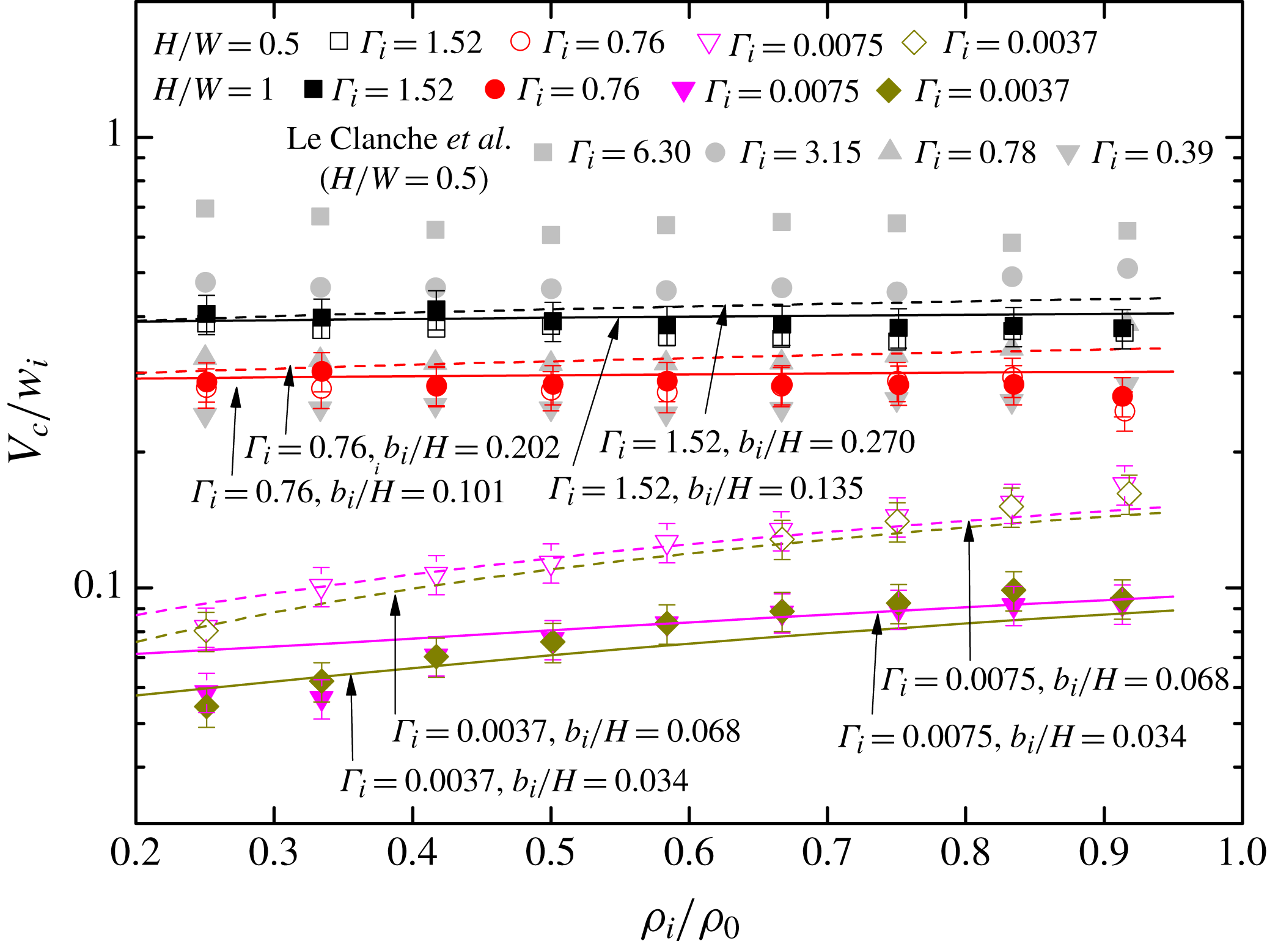
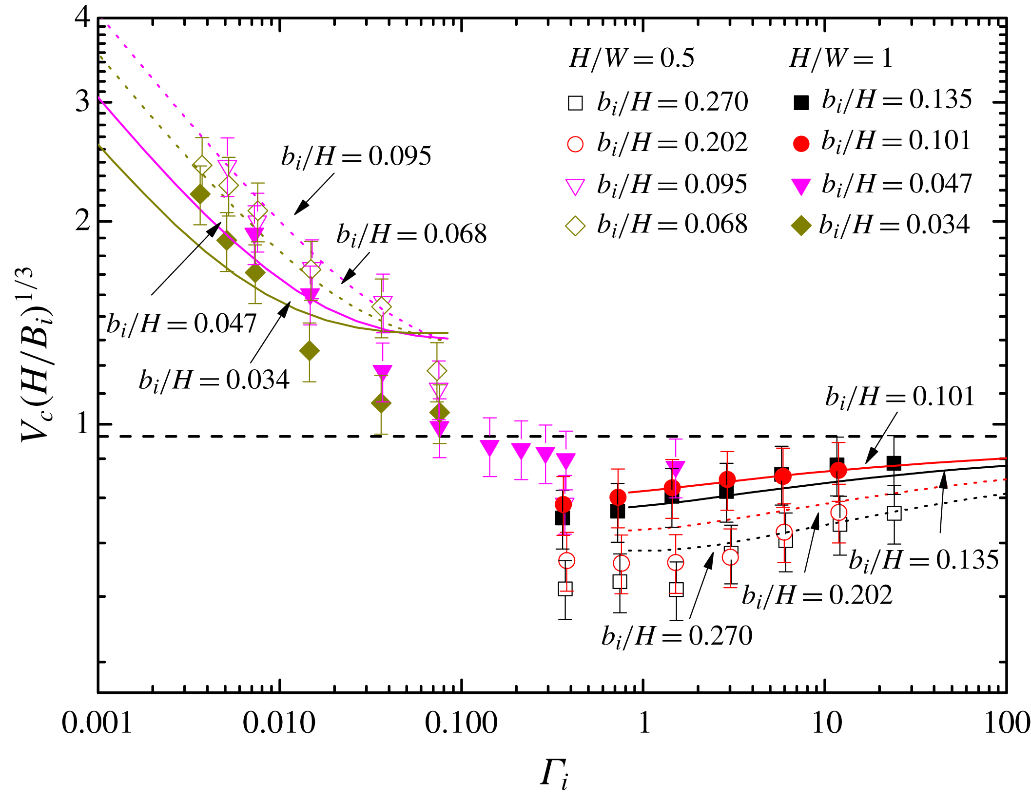
Our experimental results are shown in figures 4 and 5. For comparison, these figures also show the data obtained by Le Clanche et al. (Reference Le Clanche, Salizzoni, Creyssels, Mehaddi, Candelier and Vauquelin2014) in a reduced-scale physical model with aspect ratio
 $H/W=0.5$
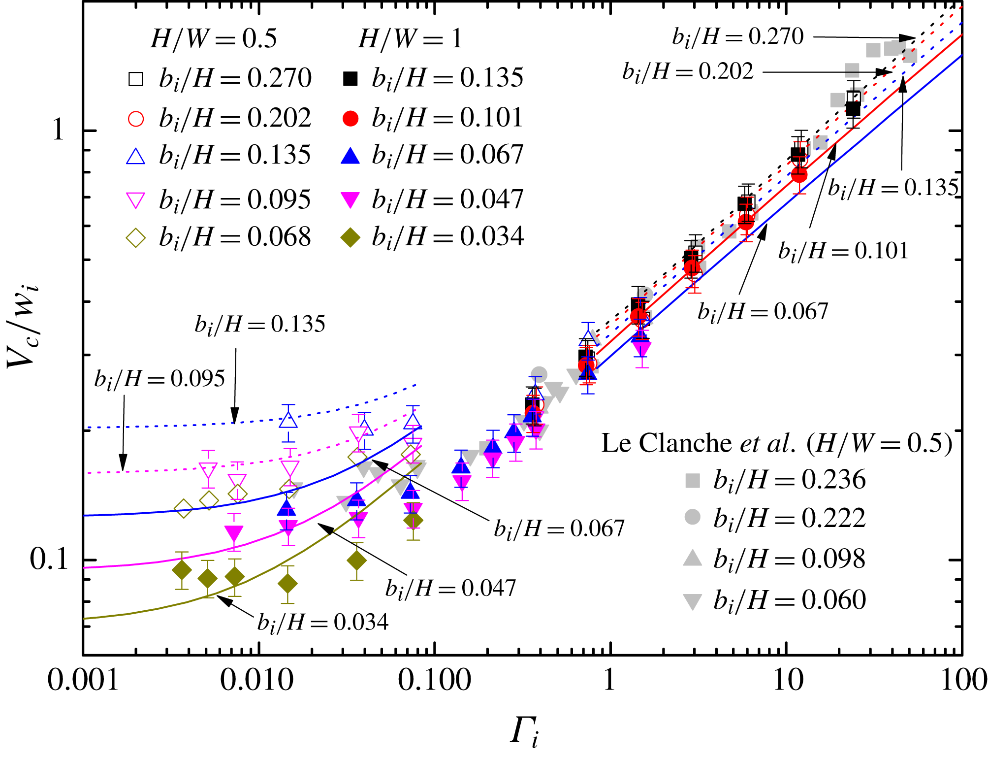
, slightly different from the model used here, and equipped with different instrumentation. Figure 4 shows the dependence of the dimensionless critical velocity on the source Richardson number, for varying source width
 $b_{i}/H$
and a fixed density ratio of
 $\unicode[STIX]{x1D70C}_{i}/\unicode[STIX]{x1D70C}_{0}=0.7$
. Figure 5 shows the influence of the density ratio on a series of releases with fixed
 $\unicode[STIX]{x1D6E4}_{i}$
, each of which has the same width
 $b_{i}/H$
.
Experimental results for
 $\unicode[STIX]{x1D6E4}_{i}>0.1$
, i.e. spanning marginally forced, through to lazy releases agree well with the data obtained by Le Clanche et al. (Reference Le Clanche, Salizzoni, Creyssels, Mehaddi, Candelier and Vauquelin2014) and confirm their main findings, namely that the dimensionless critical velocity: (i) does not show a clear dependence on the density ratio
 $\unicode[STIX]{x1D70C}_{i}/\unicode[STIX]{x1D70C}_{0}$
, whereas (ii) it clearly exhibits a dependence on the plume Richardson number. In other words, as the release becomes increasingly less forced so the critical velocity increases.
Dimensionless critical velocity as a function of plume source Richardson number
 $\unicode[STIX]{x1D6E4}_{i}$
for a fixed density ratio of
 $\unicode[STIX]{x1D70C}_{i}/\unicode[STIX]{x1D70C}_{0}=0.7$
. Comparison between experimental data (symbols) obtained for different aspect ratios
 $b_{i}/H$
and analytical solution (2.17) (lines).

Dimensionless critical velocity as a function of plume density ratio
 $\unicode[STIX]{x1D70C}_{i}/\unicode[STIX]{x1D70C}_{0}$
for different
 $\unicode[STIX]{x1D6E4}_{i}$
. Comparison between experimental data (symbols) obtained for different aspect ratios and analytical solution (2.17) (lines).

Extending the investigation to
 $\unicode[STIX]{x1D6E4}_{i}<0.1$
reveals further interesting features. Firstly we observe a weakening of the dependence of the dimensionless critical velocity on
 $\unicode[STIX]{x1D6E4}_{i}$
. This weakening is in accordance with the scaling given by the simple dimensional argument, which indicates
 $V_{c}/w_{i}\sim \text{const.}$
as
 $\unicode[STIX]{x1D6E4}_{i}\rightarrow 0$
(for any fixed pair
 $b_{i}/H$
and
 $\unicode[STIX]{x1D70C}_{i}/\unicode[STIX]{x1D70C}_{0}$
). The dimensionless critical velocity exhibits a clear systematic variation with
 $b_{i}/H$
as
 $\unicode[STIX]{x1D6E4}_{i}\rightarrow 0$
(figure 4), in which the critical velocity increases with increasing
 $b_{i}/H$
. Evidently the influence of
 $b_{i}/H$
diminishes for
 $\unicode[STIX]{x1D6E4}_{i}>0.1$
. As already noted, the investigation on the role of
 $b_{i}/H$
for large
 $\unicode[STIX]{x1D6E4}_{i}$
was limited by the constraints imposed by the experimental set-up. Data on highly forced releases also reveals a clear dependence of the dimensionless critical velocity on the density ratio (figure 5) – as the plume becomes increasingly non-Boussinesq at source (
 $\unicode[STIX]{x1D70C}_{i}/\unicode[STIX]{x1D70C}_{0}$
decreasing) so
 $V_{c}/w_{i}$
decreases. This effect, which is not evident in the data set of Le Clanche et al. (Reference Le Clanche, Salizzoni, Creyssels, Mehaddi, Candelier and Vauquelin2014), is observed only for momentum-dominated releases and becomes undetectable as
 $\unicode[STIX]{x1D6E4}_{i}>0.1$
. This suggests that, somehow counter-intuitively, as far as the critical velocity is concerned, non-Boussinesq effects have a significant dynamical effect only in the case of suitably highly forced, i.e. momentum-dominated, releases and become negligible as buoyancy begins to dominate the plume dynamics at source. In effect then, increasingly buoyancy-dominated releases lose information about the source conditions, notably concerning density. This can be physically interpreted as the effect of the plume necking and the enhanced mixing in the very near field of the source, owing to the laziness of the plume (Hunt & Kaye Reference Hunt and Kaye2005; Carlotti & Hunt Reference Carlotti and Hunt2017; Marjanovic, Taub & Balachandar Reference Marjanovic, Taub and Balachandar2017).
Further insight into the functional dependence (2.3) is provided by the comparison between the experimental results and the analytical solution (2.17). It is worth noting that plotting the theoretical predictions across the whole range of
 $\unicode[STIX]{x1D6E4}_{i}$
that was investigated, (figure 4) would require one to specify both the dependence
 $C=C(\unicode[STIX]{x1D6E4}_{i})$
and, in order to achieve reliable solutions of the plume equations (2.13), a dependence of the entrainment coefficient on the local plume Richardson number in (2.13) (Ezzamel et al.
Reference Ezzamel, Salizzoni and Hunt2015; van Reeuwijk et al.
Reference van Reeuwijk, Salizzoni, Hunt and Craske2016; Carlotti & Hunt Reference Carlotti and Hunt2017; Craske, Salizzoni & van Reeuwijk Reference Craske, Salizzoni and van Reeuwijk2017). Taking into account these dependencies would have, however, precluded our obtaining an analytical expression for the dimensionless critical velocity
 $V_{c}/w_{i}$
and the insights those simplified solutions offer. Plotting the analytical solution (2.17) requires values for
 $C_{F}$
and
 $C_{L}$
, which were obtained by fitting the data in the momentum-driven regime, i.e. for
 $\unicode[STIX]{x1D6E4}_{i}<0.1$
, and in the buoyancy-driven regime, i.e. for
 $\unicode[STIX]{x1D6E4}_{i}>1$
, respectively. This gave a value of
 $C_{F}=0.70$
for forced releases and
 $C_{L}=0.44$
for lazy releases.
In a general way, the difference between the values of
 $C_{F}$
and
 $C_{L}$
is consistent with the idea that
 $\unicode[STIX]{x1D711}$
and
 $\unicode[STIX]{x1D6FE}$
are order one quantities, exhibiting a limited variation on the plume conditions at impingement, i.e. on
 $\unicode[STIX]{x1D6E4}_{H}$
. It is however of note that the variation of the values of
 $C_{F}$
and
 $C_{L}$
are likely to incorporate the effect of the dependence
 $\unicode[STIX]{x1D6FC}=\unicode[STIX]{x1D6FC}(\unicode[STIX]{x1D6E4})$
that we have neglected in our computations. This feature was actually verified on computing the dimensionless critical velocity based on
 $\unicode[STIX]{x1D6FC}_{p}$
taking a notional minimal value (
 $\unicode[STIX]{x1D6FC}_{p}=0.6$
as a characteristic value for non-buoyant jets) and a notional maximal value (
 $\unicode[STIX]{x1D6FC}_{p}=0.12$
as the chosen reference value for plumes). The results show indeed that the effect of a varying value of
 $\unicode[STIX]{x1D6FC}_{p}$
can be fully compensated by slight variations of the values of
 $C_{F}$
and
 $C_{L}$
.
Assuming that
 $\unicode[STIX]{x1D711}$
is less sensitive than
 $\unicode[STIX]{x1D6FE}$
to
 $\unicode[STIX]{x1D6E4}_{H}$
, the difference between
 $C_{F}$
and
 $C_{L}$
implicitly implies a smaller head-loss coefficient
 $\unicode[STIX]{x1D6FE}$
for strongly jet-like impingements than for pure plume-like impingements. This latter feature is consistent with the idea that, for plume-like impingements, the volume of fluid in the impingement region (cf. shaded region in figure 2) can induce a generation of momentum owing to its buoyancy, which would result in reduced momentum losses, and therefore in an increase in the head-loss coefficient
 $\unicode[STIX]{x1D6FE}$
.
For the momentum-dominated releases, the experimental conditions generally meet the assumptions adopted in the formulation of our model, namely a small source diameter (compared to tunnel width and height) and a velocity that significantly exceeds the ventilating flow. Focusing on the results for these releases, we note a generally good agreement between the analytical solution (2.17) and the experimental data: (i) the model captures well both the dependence on the source radius
 $b_{i}/H$
(figure 4) and density ratio
 $\unicode[STIX]{x1D70C}_{i}/\unicode[STIX]{x1D70C}_{0}$
(figure 5) and, (ii) when evaluated across the data sets we collected (i.e. considering results for a fixed
 $\unicode[STIX]{x1D6E4}_{i}$
or a fixed density ratio), the average differences between model and experiments vary between 4 % and 10 %. These therefore do not exceed the experimental uncertainties.
 $V_{c}(H/B_{i})^{1/3}$
as a function of
 $\unicode[STIX]{x1D6E4}_{i}$
. The dashed horizontal line plots the large-
 $\unicode[STIX]{x1D6E4}_{i}$
solution
 $V_{c}(H/B_{i})^{1/3}=\widehat{\text{Fr}}_{c}$
, equation (2.22), for the asymptotic critical Froude number
 $\widehat{\text{Fr}}_{c}=(25/48\unicode[STIX]{x03C0}\unicode[STIX]{x1D6FC}_{p}^{2})^{1/3}C_{L}=0.95$
.

For buoyancy-dominated releases, the values of the control parameters in the experiments are instead clearly beyond the range of validity of the model, both for the source radius (
 $b_{i}/H$
) and velocity, since
 $w_{i}\simeq V_{c}$
. Despite this, the model captures well (the differences are again in the range of 4 % to 10 %) the general dependency of the dimensionless critical velocity on
 $\unicode[STIX]{x1D6E4}_{i}$
(figure 4) and the negligible role of the density ratio (figure 5). Concerning the effect of the source radius, the comparison between predictions and experimental data (figure 4) is less instructive. To discover the role of the source radius
 $b_{i}$
for highly lazy releases a different scaling needs to be adopted. We refer to the scaling suggested by the asymptotic solution (2.22), valid as
 $\unicode[STIX]{x1D6E4}_{i}\rightarrow \infty$
, a scaling that would be expected for releases that approximate to point sources of ‘pure’ buoyancy. The rescaled data is presented in figure 6 where we also plot the value of
 $\widehat{\text{Fr}}_{c}$
predicted theoretically (dotted line); taking
 $\unicode[STIX]{x1D6FC}_{p}=0.12$
and
 $C_{L}=0.44$
gives
 $\widehat{\text{Fr}}_{c}=0.95$
. The normalisation of
 $V_{c}$
by
 $(B_{i}/H)^{1/3}$
is clearly not expected to be appropriate for momentum-dominated releases, which explains the considerable scatter of the data for low
 $\unicode[STIX]{x1D6E4}_{i}$
. The normalised critical velocity for pure and lazy plumes is shown to be significantly lower than the asymptotic value of the critical Froude number
 $\widehat{\text{Fr}}_{c}$
. Data for
 $H/W=0.5$
lies systematically below the data obtained for
 $H/W=1.0$
, clarifying the influence of source width
 $b_{i}/H$
. Notably, the variation with
 $b_{i}/H$
is captured well by the theory even for values of
 $b_{i}/H$
for which
 $b_{i}\not \ll W$
(e.g.
 $b_{i}/H=0.270,0.202,0.135$
). Both sets of data (
 $H/W=0.5$
and
 $H/W=1$
) gradually approach the asymptotic value and the predictions agree well with both sets of data. Since the model represents the buoyant release as a plume in a laterally unbounded cross-flow, the predictions do not include any influence of a varying tunnel aspect ratio. This good agreement with the experimental data therefore suggests that, in the range of source widths investigated, the confinement of the ventilation flow by the lateral tunnel walls has little influence on the critical velocity. We anticipate that confinement may play a role in the interaction between the ventilation flow and the releases with increasing source width. This is likely to result in a modification of the entrainment of ambient air into the plume and in an increase in the drag coefficient. For a given ventilation velocity, this would, in turn, increase the inclination of the trajectory of the rising buoyant fluid. Note, however, that an enhanced bending of the plume will have no effect on the critical velocity, according to the definition adopted here, which does not take into account the location of the impingement point (with respect to the source) of the buoyant release on the ceiling. Concerning the effect on the entrainment process, as quantified by the entrainment coefficient, it is of note that its variation acts through a negative two-thirds power (see (2.22)), and this coefficient is therefore not expected to play a major role in affecting the critical velocity (a 50 % modification of the entrainment coefficient would imply a 25 % modification of the critical velocity).
5 Conclusions
We have investigated the dynamics of a release of buoyant fluid steadily discharged from a circular source located at the centre of a longitudinally ventilated tunnel that gives rise to a turbulent jet-like or plume-like flow. In particular, we focused on the dependence of the so-called ‘critical ventilation velocity’
 $V_{c}$
, that confines the buoyant fluid downwind of the release point, on conditions at the source, exploring the role of the injection velocity
 $w_{i}$
, density of the release fluid
 $\unicode[STIX]{x1D70C}_{i}$
relative to the ambient
 $\unicode[STIX]{x1D70C}_{0}$
, and source radius
 $b_{i}$
. By assuming negligible diffusive effects, the dimensionless critical velocity
 $V_{c}/w_{i}$
has been shown to depend on four dimensionless groups: the plume source Richardson number
 $\unicode[STIX]{x1D6E4}_{i}$
, the dimensionless source radius
 $b_{i}/H$
, the tunnel aspect ratio
 $H/W$
and the density ratio
 $\unicode[STIX]{x1D70C}_{i}/\unicode[STIX]{x1D70C}_{0}$
. The latter ratio is particularly relevant in regard to dynamical effects, known as non-Boussinesq, in which there are large density differences between the buoyant emission and ambient fluid.
To investigate these dependencies, we performed experiments in a reduced-scale tunnel, where buoyant releases were produced with a mixture of helium and air. Experiments have shown the following main features:
(i) the dependence of
 $V_{c}/w_{i}$
on
$\unicode[STIX]{x1D6E4}_{i}$
reveals the existence of two flow regimes, one for
$\unicode[STIX]{x1D6E4}_{i}\ll 1$
and one for
$\unicode[STIX]{x1D6E4}_{i}\gg 1$
;
(ii) the transition between the two regimes occurs in the range
$10^{-2}<\unicode[STIX]{x1D6E4}_{i}<1$
;(iii)
$V_{c}/w_{i}$
does not show a dependence on the density ratio for
$\unicode[STIX]{x1D6E4}_{i}>0.1$
, whereas for lower
$\unicode[STIX]{x1D6E4}_{i}$
the dependence is of the form
$(\unicode[STIX]{x1D70C}_{i}/\unicode[STIX]{x1D70C}_{0})^{1/2}$
; and(iv) in the range of source radii investigated,
$V_{c}/w_{i}$
is more sensitive to
$b_{i}/H$
for forced releases (
$\unicode[STIX]{x1D6E4}_{i}<1$
) than for lazy releases (
$\unicode[STIX]{x1D6E4}_{i}>1$
).


To obtain further insight into the flow dynamics we interpreted the experiments by comparing their results to an analytical solution of a simplified model of a top-hat plume in a cross-flow, which was formulated following the well established approach of Morton et al. (Reference Morton, Taylor and Turner1956). Despite its simplicity and the constraining assumptions on which it is based (assumptions which do not hold in every experiment, especially for buoyancy dominated releases at source) the model is able to capture the main trends identified by the experiments, namely the existence of two flow regimes, and the onset of non-Boussinesq effects for sufficiently highly forced releases only,
 $\unicode[STIX]{x1D6E4}_{i}<0.1$
. In the case of the momentum-dominated releases, the model aids in the elucidation of the role of the source radius
 $b_{i}/H$
and of the density ratio
 $\unicode[STIX]{x1D70C}_{i}/\unicode[STIX]{x1D70C}_{0}$
on the flow dynamics. Notably, these dependencies are highlighted by the asymptotic solution obtained in the limit
 $\unicode[STIX]{x1D6E4}_{i}\rightarrow 0$
. According to the asymptotic solution,
 $V_{c}/w_{i}$
is shown to depend on
 $(\unicode[STIX]{x1D70C}_{i}/\unicode[STIX]{x1D70C}_{0})^{1/2}$
, although it does not fully rescale on it. Note that the model also captures well the trend of the results for lazy releases, even though these latter are characterised by experimental conditions that do not generally meet the assumptions adopted in the model, namely that of a ‘small’ source (i.e.
 $b_{i}\ll H$
) and of an emission in a weak ventilation flow, i.e.
 $V_{c}\ll w_{i}$
. This good agreement between model and experimental data for lazy releases (which are emitted by the larger sources in the experiments), and collected for two different aspect ratios of the tunnel section, further suggests that, for the range of source radii investigated here (i.e.
 $b_{i}\leqslant 0.54W$
), the lateral walls have a limited influence on the critical ventilation condition.
An overall conclusion that we may draw is that for buoyancy-dominated releases the critical velocity does not exhibit a dependence on the ratio of the source to ambient density. This feature, which was not at all clear at the outset, supports the use of simplified mathematical models for the first-order prediction of buoyant flows in ventilated spaces.
Acknowledgement
L.J. gratefully acknowledges the support of the China Scholarship Council.