II. Literature Review

We draw upon the hedonic price literature for wine and the two-tier stochastic frontier literature. As far as we know, we are the first to investigate a two-tier stochastic frontier price equation for wine, although Storchmann, Mitterling, and Lee (Reference Schnabel and Storchmann2012) use a two-step procedure and regress residuals on winery characteristics. We begin with an overview of wine pricing and then turn to reviews of the academic literature on hedonics and some previous uses of the two-tier stochastic frontier model.

Bidmead (Reference Bidmead, Özer and Phillips2012) explains the intricacies of wine pricing in the United States. Although the empirical academic work ignores many of the practical details, it is useful to understand the institutional framework that challenges wine producers in the field. Wine pricing is a complex art, much less straightforward than pricing for typical agricultural commodities. The retail price of a 750 ml bottle of wine can range from a few dollars to more than a thousand dollars per bottle. Bidmead (Reference Bidmead, Özer and Phillips2012) discusses the many factors entering the pricing decision such as production techniques, packaging, vineyard location, scarcity of specific grape varieties, consumer dynamics, channel dynamics, and competition. Wine production involves growing the grapes under particular meteorological conditions combined with the expertise of the winemaker intertwined with reputation effects. Wine is a heterogeneous experience good. These considerations complicate the estimation of a hedonic price equation.

At the most general level, the cost of the grapes determines the price of a bottle of wine. The rule of thumb is that the price of a bottle of wine is 1% of the cost per ton of the grapes. Grapes that sell for $200 per ton translate into a $2 bottle of wine; grapes that sell for $6,000 per ton translate into a $60 bottle of wine (Bidmead, Reference Bidmead, Özer and Phillips2012). However, this is just the beginning. There are additional considerations: (1) Consumers perceive price to be a signal of quality so consumers will pay more for a more expensive bottle of wine because it has a higher price, ceteris paribus. (2) Location is a signal of quality—in the United States, there are designated geographies such as Napa, Russian River, or the Stag's Leap District. (3) Wine magazines (e.g., Wine Spectator) and wine critics (e.g., Robert Parker) rate wines and these ratings influence the price. (4) Red wines tend to have a higher price than white wines. (5) Wine prices tend to be relative to a benchmark that consists of other wines from the same geographic region with similar characteristics. This is analogous to pricing houses based upon comparable houses. For further details, see Bidmead (Reference Bidmead, Özer and Phillips2012). He concludes that wine pricing is a strategy and an art. Empiricists who embrace the challenge of estimating a hedonic price equation with quantitative proxies for soft concepts (taste, reputation) should expect challenge and controversy. We move forward with the added challenge of introducing the two-tiered stochastic frontier technique to the mix.

Estimating a relationship between price and the characteristics of a good goes back to Waugh (Reference Waugh1928), who considers vegetables and quality. Lancaster (Reference Lancaster1966) revisits demand theory in terms of characteristics and provides a theoretical justification for hedonic analysis. However, Rosen (Reference Rosen1974) points out that observed prices reflect supply and demand influences, corresponding to the intersection of consumer bid functions and supplier offer functions. Extrinsic and intrinsic factors influence consumers and producers. In wines, extrinsic factors are grape variety, reputation, marketing, and the quality of wine production. Intrinsic factors include subjective sensory factors such as the bouquet, taste, color, balance, and complexity.

Consumer bid functions and supplier offer functions for sensory factors increase at a decreasing rate. Consumers are willing to pay a higher price only for a greater sensory experience; suppliers are willing to produce a greater sensory experience only for a higher price. At equilibrium, bid and offer functions for the sensory experience are tangent, given extrinsic factors. The market data captures these points of equilibrium where producer and consumer valuations are reconciled (Oczkowski and Doucouliagos, Reference Oczkowski and Doucouliagos2014).

A further complication in estimating hedonic price equations for wine is the interplay between price and sensory measures. Consider some of these complicating factors: (1) Wine critics rate wines after the producer releases the wine with a recommended retail price. The price and the rating might be inconsistent, resulting in wines that are overpriced and underpriced. (2) Consumers may use the price as well as the extrinsic and intrinsic factors as a measure of quality. (3) Consumers are less sophisticated judges of wine quality than wine critics, and might buy based upon ratings. (4) Wine critics might disagree and even a given critic might be inconsistent over time. (5) It is possible that the critics are evaluating quality based upon a set of metrics that do not correspond to the preferences of less sophisticated consumers.

Research on the determinants of wine prices finds conflicting evidence on the importance of extrinsic and intrinsic (sensory) factors. For a discussion of extrinsic factors based upon information on the bottle using data for Australian wines in the British wine market, see Steiner (Reference Steiner2004). Perrouty, d'Hauteville, and Lockshin (Reference Perrouty, d'Hauteville and Lockshin2006) find that region of origin is important, particularly for more sophisticated consumers, based upon survey data for European wines. Combris, Lecocq, and Visser (Reference Combris, Lecocq and Visser1997) conclude that extrinsic factors are most important for Bordeaux wines.

There is extensive work on the contribution of the tasting score to the price of a bottle of wine. Storchmann (Reference Storchmann2012) summarizes the relationship between expert ratings and wine prices, identifies various flaws in expert rating, but none-the-less concludes that wine consumers rely on these ratings in their purchase decisions. Because wine is an experienced good, its characteristics are not known to most wine drinkers before consumption, and, thus, ratings can help fill an information void. Ashenfelter (Reference Ashenfelter2008) shows that expert opinion regarding Bordeaux vintage qualities can be seriously flawed. Yet in another article, Ashenfelter and Jones (Reference Ashenfelter and Jones2013) regress Bordeaux wine prices on ratings and separately prices on vintage, weather information, and find that both are good predictors of wine prices. When they regress wine prices on both expert ratings and weather information, however, the expert ratings became statistically insignificant. The implication is that weather information contains information that is more complete. None-the-less, ratings condense the detailed information into a single value index; this single value index is not expected to transmit the full information set of determining factors to wine quality. Landon and Smith (Reference Landon and Smith1997) do, however, find a positive relationship between the quality ratings for Bordeaux wine in Wine Spectator and Bordeaux wine prices. A similar positive relationship between ratings and prices is reported by Benjamin and Podolny (Reference Benjamin and Podolny1999) for Californian wines, and by Schamel and Anderson (Reference Schamel and Anderson2003) for Australian and New Zealand wines. Ratings might not be the sole price predictor, but they contain information and are positively correlated with prices.

Constanigro, McCluskey, and Mittelhammer (Reference Constanigro, McCluskey and Mittelhammer2007) use Wine Spectator data as we do and estimate hedonic equations for red and white wines. They conclude that the wine market is differentiated into multiple segments or wine classes. This supports our use of only U.S. Rieslings in our hedonic estimation. They also conclude that rating by specialized magazines were significant factors in determining wine prices and should be included in a hedonic model. They argue that only a small percentage of wine purchasers are connoisseurs, and ratings provide a signal to these consumers. In a further study, Chen and McCluskey (Reference Chen and McCluskey2018) also use Wine Spectator data to investigate the impact of tasting scores as well as tasting notes in a hedonic wine equation for Washington state red wines. They find that tasting score is an important determinate of wine price, but that attributes from the tasting notes, especially reference to cherry, spice, and tannin, are also important in the high-price wines. Similarly, Caudill and Mixon (Reference Caudill and Mixon2016) use a class-specific mixture hedonic model to estimate wine prices to address the issue that among the price breaks in wine, substantial product attributes might exist. They use data on California and Washington state red wines and find four classes where the impact of the explanatory variables, including the tasting score varied.

Oczkowski and Doucouliagos (Reference Oczkowski and Doucouliagos2014) summarize these and other studies in a comprehensive analysis of more than 180 articles over 20 years that estimate a hedonic price equation for wine. They conduct a meta-regression analysis with a particular focus on the relationship between wine prices and quality ratings. The partial correlation coefficient is positive 0.30. The authors interpret this result to suggest that there are “strategic buying opportunities for better-informed consumers.” We find this result to be heartening since the contribution of the two-tier stochastic frontier is to identify these underpriced and overpriced wines.

There is extensive literature on the efficiency of ratings, based largely upon Bordeaux price data (Dubois and Nauges, Reference Dubois and Nauges2010). This is understandable given the investment opportunities that exist in the Bordeaux market. However, most of the tasting and ratings occur when the wine is young and not ready to drink, which introduces errors in the assessment. We focus on Rieslings, which do not need to be aged. What you taste shortly after release reflects the evaluation unless the wine is not drunk soon enough.

Polachek and Yoon (Reference Polachek and Yoon1987) apply their two-tier model to the labor market, where their over and under estimates reflect the relative bargaining power of employers and employees in an equilibrium. Kumbhakar and Parmeter (Reference Kumbhakar and Parmeter2009) as well as Blanco (Reference Blanco2017), similarly look at the labor market and generally find employers with the bargaining power. Other applications include tourist bargaining (Zhang et al., Reference Zhang, Zhang, Yang and Zhou2018), who find that tourist traveling with companions and who obtain travel information from friends and mass media have better bargaining power over sellers. A real estate application by Xu et al. (Reference Xu, Wang, Zhou and Geng2016) finds that Chinese buyers pay a price above the hedonic expected price. None of the limited applications involves wine or any other agricultural commodity. We believe this is an overlooked opportunity.

III. Methodology Estimating Overpricing and Underpricing

The two-tier method developed by Polachek and Yoon (Reference Polachek and Yoon1987) was used to obtain estimates of the expected price of wine as well as overpricing and underpricing. This method estimates an expected price function, with estimation and decomposition of the residual into three components. The first component is a normal random error. The second and third components of the residual are additional distributions above and below the expected function in addition to the normal random error. To ensure identification separate from the normal error, these second and third components are specified as exponential distributions. Estimation is by maximum likelihood.

The equation for the i _th observation is

(1)$$y_i = \; x_i^{\prime} \delta \, + \, \varepsilon _i \comma$$

where y _i is the dependent variable, x _i is the vector of covariates, δ is the corresponding parameter vector, and ε _i = v _i – u _i + w _i, representing the composite error term and v is a symmetric normal distribution, u an exponential distribution below the regression equation, and w an exponential distribution above the regression equation. The variable u represents underpricing and the variable w represents overpricing, controlling for the variables in the expected component of the regression equation.

Polachek and Yoon (Reference Polachek and Yoon1987) and Kumbhakar and Parmeter (Reference Kumbhakar and Parmeter2009) derive the probability density function of ε _i and the resultant log likelihood function to estimate the parameter vector δ as well as the parameters of the normal and the two exponential functions as

(2)$$lnL\lpar {x;\theta} \rpar = \; -n\lpar {\sigma_u + \sigma_w} \rpar + \; \mathop \sum \limits_{i = 1}^n ln[e^{\alpha _{i\;}} \Phi \lpar {\beta_i} \rpar + e^{a_{i\;}} \Phi \lpar {b_i} \rpar ]\comma $$

where θ = (δ. σ _v, σ _u, σ _w) and

$$a_i = \displaystyle{{\sigma _v^2} \over {2\sigma _w^2}} -\varepsilon _i/\sigma _w{\rm \;} \ \ \alpha _i = \displaystyle{{\varepsilon _i} \over {\sigma _u}} + \displaystyle{{\sigma _v^2} \over {2\sigma _u^2}} {\rm \;} \ \ b_i = \displaystyle{{\varepsilon _i} \over {\sigma _v}}-\sigma _v/\sigma _{w\;} $$

$$\beta _i = -\left( {\displaystyle{{\varepsilon_i} \over {\sigma_v}} + \sigma_v/\sigma_u} \right).$$

From these estimates the conditional distributions for u _i and w _i can be derived as

(3)$$E\left( {\displaystyle{{u_i} \over {\varepsilon_i}}} \right) = \displaystyle{1 \over \lambda} + \exp \lcub {\alpha_i-a_i} \rcub \sigma _v [{\phi \lpar {-\beta_i} \rpar + \beta_i{\rm \Phi} \lpar {\beta_i} \rpar }] /\chi _{1i}$$

(4)$$E\left( {\displaystyle{{w_i} \over {\varepsilon_i}}} \right) = \displaystyle{1 \over \lambda} + \sigma _v [{\phi \lpar {-b_i} \rpar + b_i{\rm \Phi} \lpar {b_i} \rpar }] /\chi _{1i} \comma$$

where $\lambda = \displaystyle{1 \over {\sigma _u}} + \displaystyle{1 \over {\sigma _w}}\; $ and χ _1i = Φ(b _i) + exp{α _i−a _i}Φ(β _i).

Notice that because the expected values of u and w are conditional upon the total error, and because the expected component of the regression is estimated with error such that the regression can overlap both the u and w distributions, each observation has an estimate of both overpricing and underpricing.

Finally, because the dependent variable is in logarithmic form, an exact percentage of overpricing or underpricing is obtained as:

(5)$$PercentOver = 100 [{e^{E\lpar {u_i/\varepsilon_i} \rpar }-1}] $$

(6)$$PercentUnder = 100 [{e^{E\lpar {w_i/\varepsilon_i} \rpar }-1}] $$

Maximum likelihood estimates of the parameters in θ are obtained in Stata using the ado file “twotier” written by Hung-Jen Wang.Footnote ¹ Given that we specify exponential functions for the overpricing and underpricing errors, with a change in signs, and that the random error is normally distributed, the parameters of the maximum likelihood Equation (2) are identifiable (Kumbhakar and Parmeter, Reference Kumbhakar and Parmeter2009). Those parameters are used to mathematically derive estimates of the overpricing and underpricing.

However, if the data does not support the existence of concurrent overprice and underprice estimates, then no solution is attainable because the model specifies simultaneously both the existence of an overprice and an underprice. It is possible that an underprice or overprice estimate occurs separately. Either of those can be estimated using a traditional stochastic frontier specification with a one-sided term in addition to a random error.

To estimate the potential and amount of overpricing only, Equation (1) is again estimated but with the error structure specified as ε _i = v _i + w _i. For underpricing, Equation (1) is also estimated but with the error structure specified as and ε _i = v _i – u _i. These models are analogous to the Stochastic Frontier Analysis (SFA) cost efficiency model for overpricing, and the SFA production efficiency model for underpricing (Kumbhakar and Lovell, Reference Kumbhakar and Knox Lovell2000). Consistent with the two-tier model estimation, the efficiency error term is defined and estimated as an exponential functional form.

The one-sided estimate for the underpricing u _i is:

(7)$$lnL\lpar {x;\theta} \rpar = \mathop \sum \limits_{i = 1}^n \left [{-\ln \sigma_u + \displaystyle{{\sigma_v^2} \over {2\sigma_u^2}} + \ln \Phi \left( {-\; \displaystyle{{\varepsilon_i} \over {\sigma_v}}-{\displaystyle{{\sigma_v} \over {\sigma_u}}}_{}} \right) + \; \displaystyle{{\varepsilon_i} \over {\sigma_u}}\;} \right]$$

The estimate for the overpricing w _i is:

(8)$$lnL\lpar {x;\theta} \rpar = \mathop \sum \limits_{i = 1}^n \left [{-\ln \sigma_w + \displaystyle{{\sigma_v^2} \over {2\sigma_w^2}} + \ln \Phi \left( { + \displaystyle{{\varepsilon_i} \over {\sigma_v}}-{\displaystyle{{\sigma_v} \over {\sigma_w}}}_{}} \right)-\; \displaystyle{{\varepsilon_i} \over {\sigma_w}}\;} \right]$$

The extent of underpricing and overpricing is then calculated as specified by Kumbhaker and Lovell (Reference Kumbhakar and Knox Lovell2000).

IV. Data and Results

A. Data

Riesling wine data are from the Wine Spectator's website, which contains more than 372,000 wine ratings.Footnote ² Only data for U.S. Rieslings for the vintage years from the new century of 2000 through 2016 are used. Ice wines, mostly in 375 ml bottles, and wine in 1.5-liter bottles were both deleted from the data. The data consists of the complete name of the wine, vintage year, release price, viticulture area, the number of cases produced, drink by year date, and the tasting score as determined by the Wine Spectators tasting panel for Riesling wines from across the United States.Footnote ³ Some data fields, such as the number of “cases produced” and “drink by year,” are incomplete for many observations.

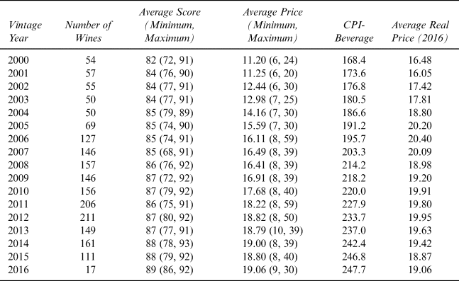
Table 1 contains a summary of the data by year. There are 1,922 observations from 792 wineries. The number of wines evaluated increases by year, with a peak number of 206 U.S. Rieslings evaluated in the year 2011. The tasting scores for these Rieslings averages 82 in 2000 and increases to 89 by 2016. Our interpretation is that U.S. Rieslings have improved over this 17-year period as reflected by an increase in the minimum score over time, rather than inflation of tasting scores by the panel. It is obvious, however, that the average price of these U.S. Rieslings have increased over time, from an average nominal price of $11.20 in 2000 to $19.06 by 2016. To adjust all prices to 2016 values, prices are deflated by the U.S. Consumer Price Index for all beverages and food, and the regression uses the logarithm values of deflated prices. Wine prices have also increased in real terms but less than 1% (0.6%) per year over this period, perhaps due to rising quality over time, which the tasting score should capture.

Table 1

Summary of 1,922 U.S. Riesling Wines from Wine Spectator Tastings

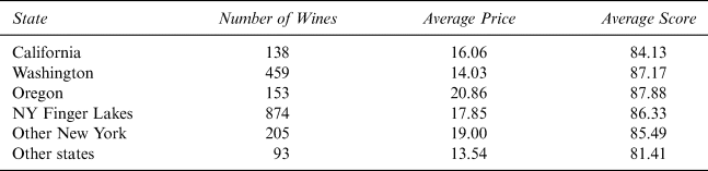
Table 2 summarizes the number of Rieslings evaluated by the major wine producing states, with New York separated into the Finger Lakes (a major Riesling producer) and the rest of New York. Of the total 1,922 Rieslings, 874 originated from the Finger Lakes Region, 205 originated from other areas of New York, 459 originated from the state of Washington, 153 originated from Oregon, and 138 originated from California. The remaining 93 Rieslings originated in other states. Rieslings from Oregon have the highest price (nondeflated), but also receive the highest-average-tasting score. Wines produced in states outside the major wine producing states receive the lowest-tasting score and are priced the lowest.

Table 2

Riesling Wine Numbers, Prices (Nominal), and Tasting Scores by State, Years 2000–2016

B. Results

Two and one-tier stochastic models are used to estimate whether wines are priced correctly. In particular, we consider the following questions: (1) Is the tasting score consistent with the release price of Riesling wines? (2) What is the influence of prestige as determined by winery regional location, on Riesling wine prices? (3) Do economies of scale influence Riesling wine prices?

(1) Is the Tasting Score Consistent with the Release Price of Riesling Wines?

The price of a bottle of wine reflects the characteristics that consumers value, tempered by supply factors. These characteristics include extrinsic factors such as reputation, region, label information, and prestige, and sensory factors such as balance, complexity, bouquet, and terroir. The sensory factors, in particular, are difficult to quantify. A tasting panel of experts scores wines and provides an overall rating. The tasting panel presumably assesses all of the taste factors that consumers value. Given the literature discussed previously, we used the tasting score and the tasting score squared as a single-value proxy for the many factors that underlie correct wine pricing. The core regression of log price against the tasting score and tasting score squared established the benchmark to identify overpricing and underpricing. If the tasting score correctly reflects all factors that underlie consumer valuation of wine, the tasting score would be a perfect predictor of expected price. However, wines could be mispriced if the tasting score fails to capture all of the attributes that consumers value and prices respond to supply considerations such as economies of scale.

There are reasons why the tasting score might misrepresent consumer valuations of the factors that are important in buying a bottle of wine. (1) The tasting panel might use a rubric that is appropriate for the sophisticated segment of the wine market, but not aligned with the preferences of ordinary wine consumers. (2) The tasting panel might be inconsistent in their evaluation of wines. (3) There are alternative tasting panels and they disagree. These considerations can produce the opportunity to purchase bargain wines and to avoid wines that have prices that are too high, particularly for discriminating consumers who “believe” the experts. However, our intent is not to arrive at a complete hedonic wine price model, but to simply determine that if a consumer is buying wine based solely on the tasting score, are some wines overpriced or underpriced, and thus bad or good bargains for that consumer?

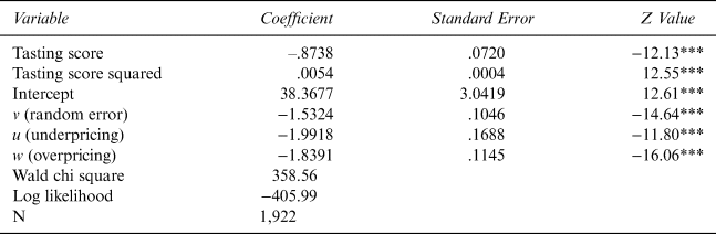
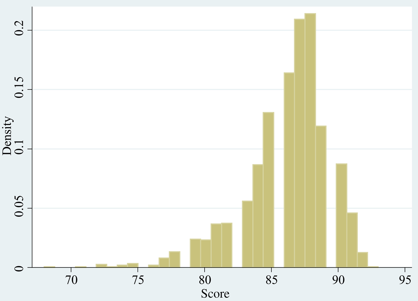
Table 3 provides the results of regressing the log of deflated bottle price against the tasting score and the tasting score squared in the two-tier stochastic model, where v is the symmetric normal error term, u is the exponential one-sided error term below the regression line (underpriced), and w is the exponential one-sided error term above the regression line (overpriced). Tasting score and tasting score squared are significant at the 1% level as are the over and under error components. However, the negative and then positive signs on the linear- and quadratic-tasting score estimated coefficients indicate a convex relationship between the price of wine and tasting score. Wine prices decrease to the tasting score of 81, with a predicted price of $20.48, and then increases to a price of $22.41 at a tasting score of 85, and $32.00 at a tasting score of 90. As shown in Figure 1 there was one wine with a low-tasting score of 68—the majority of the scores ranged over the interval of 85 through 90, with a few breaking the 90 barrier. Most wines are along the positively sloped segment of the price-tasting score relationship. Obviously, the estimates on the score variables are the result of fitting the estimated equation to the entire data and not the outliers. The result is that with an increasing predicted wine price below the score of 81, many of these low-score wines will be estimated as underpriced, when in fact they may not be underpriced. Only 4% of the wines scored lower than 81.

Table 3

Estimate of the Two-Tier U.S. Riesling Wine Pricing Model with Tasting Score and Tasting Score Squared, No Variables in Error Components

Note: *** Statistically significant at the 0.01 level.

Figure 1

Distribution of U.S. Riesling Wine Tasting Score, 2000–2016

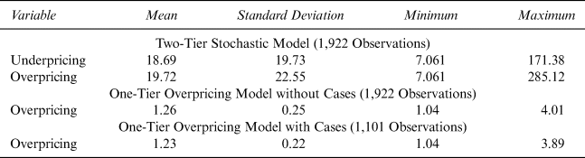
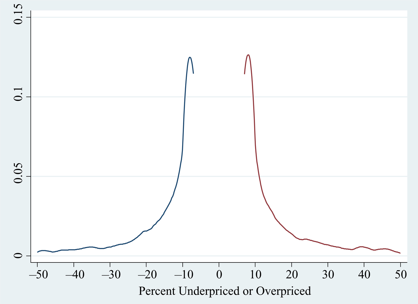
We constructed the estimates of percent overpriced and percent underpriced using Equations (5) and (6). Table 4 contains the descriptive statistics. The Riesling wines are underpriced on average by 19% and overpriced on average by 20%. One wine was underpriced by 171% and another wine was overpriced by 285%. However, given the standard deviation of 20 for the underpriced estimate and 23 for the overpriced estimate, very few wines are substantially underpriced or overpriced as illustrated by the empirical distributions of underpricing and overpricing shown in Figure 2.

Table 4

Summary Statistics of Percent of Underpricing and Overpricing of U.S. Riesling Wines, Various Specifications

Figure 2

Distribution of Riesling Wines Underpriced or Overpriced

Notes: Generated from two-tier model with tasting score and score squared only. Distributions truncated at –50 and 50% for illustration.

The tasting score is significantly correlated with wine prices, but wines are still mispriced. This might be a distortion in the wine market, or it might be attributable to the tasting score failing to correctly evaluate wine quality, missing variables that capture attributes besides tasting score that consumers value, or supply considerations.

(2) What Is the Influence of Prestige as Determined by Winery Regional Location, on Riesling Wine Prices?

U.S. Rieslings are produced in the following regions: California, Washington, Oregon, New York Finger Lakes, other New York, and rest of the United States. To the extent that region affects the taste of the wine, it should be incorporated into the tasting score. However, wine is an experience good. Drinking a bottle of wine is a multi-dimensional process that often occurs in the context of dinner with friends who enjoy the quality of the wine along with rituals surrounding the removal of the cork (or screw cap), information on the label, the sampling of the wine, and a discussion. Price may also be a component of this experience in which consumers interpret price as a measure of quality (Schnabel and Storchmann, Reference Schnabel and Storchmann2010). However, we explore the possibility that price is associated with the prestige of a region.

Wine drinkers are not typically expert tasters and use heuristics to evaluate wines. For example, dinner guests might not value a wine from North Dakota as highly as a wine from Oregon, even if both wines have the same tasting score. Since there is a prestige element to the wine drinking experience, we use region as a proxy for prestige, and test whether or not there is an impact of region on price above and beyond the influence of region on the tasting score. The assumption is that all wineries in a region capture this price premium or discount, yet some might still overprice or underprice. Individual wineries may also command a reputational price premium, but with an unbalanced data set from 792 wineries with an average of only 2.46 observations per winery, individual winery estimates would not be precise.

We added five regional dummies (omitting “rest of U.S.”) to the expected value component of the two-tier stochastic model. The model failed to solve. We also experimented with adding the regional dummies to both asymmetric error terms, since this provides more efficient estimates (Caudill and Ford, Reference Caudill and Ford1993). It is appropriate to add the dummies simultaneously to both error terms since we have no a priori reason to know in what region wineries might underprice, overprice, or both, even after capturing any regional prestige premiums or discounts. Again, the model failed to solve. The introduction of regional dummies under either specification introduced additional variables into the expected component of the function that eliminated the concavity of the maximum likelihood function required for the two-tier model to reach a solution. One could stop here, wines are mispriced for reasons discussed earlier. Consumers could overpay and underpay based upon the tasting score, and we could provide a buying guide. However, we chose to pursue the question in an attempt to explain the apparent mispricing.

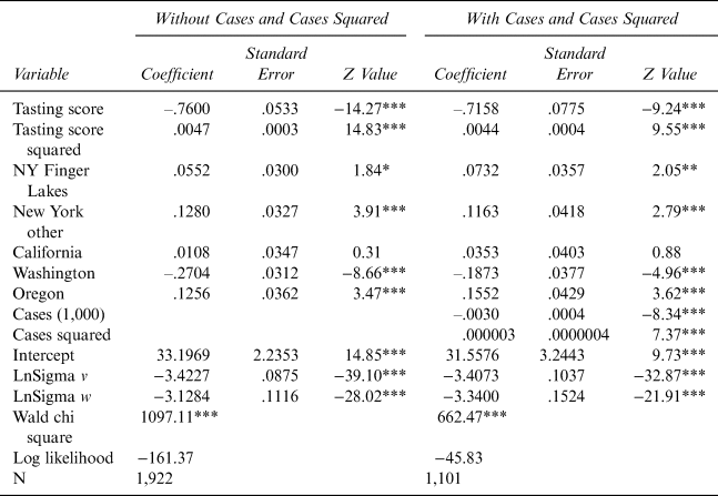
We estimated two one-tier stochastic frontiers: a stochastic cost function model analog to capture overpricing and a stochastic production function model analog to capture underpricing. Tasting score, tasting score squared, and regional dummies are included in the expected value component of the model. The one-sided error terms are exponential to maintain consistency with the two-tier model. The production function specification failed to solve, implying there is no underpricing when accounting for regional reputation. The cost function specification did reach a solution. Table 5 contains the results. We conclude that the overpricing in the two-tier model can be partially explained by the location dummies (prestige), yet additional overpricing remains. There is no evidence of underpricing in the wine market. Tasting score, tasting score squared, and all regions are statistically significant, except for California. The one-sided overpriced error is significant at the 1% level. To quantify overpricing, we constructed the variable percent overpriced, equal to predicted price minus actual price divided by actual price. Wines are overpriced on average only around 1.3% compared to 19.7% in the two-tier model without regional dummies. The regional dummies in the one-tier cost function model explain most of the previous mispricing.

Table 5

Estimate of a U.S. Riesling Wine Hedonic Pricing Model Allowing Only Overpricing (Cost Function Analog)

Notes: *, **, *** Statistically significant at the 0.10, 0.05, and 0.01 levels, respectively. No variables embedded in either of the two-error terms.

The coefficients on the regional dummies enable us to rank the prestige of the regions. New York other is the most prestigious region (12.8% premium) followed by Oregon (12.6% premium), New York Finger Lakes (5.5% premium), California (0% premium), and Washington (27% discount), all relative to the rest of the United States. If you believe the expert tasters and are not interested in impressing your guests, then the Riesling wines of Washington state are a bargain.

(3) Do Economies of Scale Influence Riesling Wine Prices?

We have data on a number of cases produced for 1,101 of the 1,922 winery observations. We added cases and cases squared to the core stochastic frontier regression with tasting score and tasting score squared and the set of regional dummies. Table 5 contains the results. All variables are statistically significant, again except for California. The coefficients on the variables in the original regression are essentially the same in the regression with cases and cases squared except for Washington, where many of the large Riesling wineries are located. The linear and quadratic coefficients imply that the wine price decreases up to a million cases and then rises. However, the median number of cases produced by the wineries is 794, and 75% of wineries produced 3,800 cases or less, so this estimate must be interpreted with caution. There is only one winery that produces over one million cases. Most wineries are arrayed around the negatively sloped portion of the function. This suggests that as wineries produce more cases, they charge a lower price. A possible explanation is that larger wineries set the release price lower given the expected tasting score and their region as a form of insurance against an inventory of unsold wine. They might also be able to set a lower price due to a lower cost of production attributable to volume.

To quantify, the extent of mispricing in the model with cases and cases squared, we calculated percentage overpriced as predicted price minus actual price divided by actual price. Table 4 contains the descriptive statistics. The percent overpriced falls from 1.26 to 1.23%. More mispricing is explained.