2.1 Code features

2.1.2 Linear stability methods – LST and LPSE

Another in-house code has been developed to perform linear stability analysis of compressible boundary layers. The code allows both a local analysis, by solving the compressible Orr–Sommerfeld equations, and a non-local one, by solving the LPSE. Once the linearized perturbation equations are derived from the Navier–Stokes equations, different assumptions can be made and the two approaches obtained.

A critical assumption in the formulation of the LST is the parallel nature of the flow, where the dependence of the basic state on the streamwise direction is neglected. Although not congruent with reality, this assumption greatly simplifies the problem. With $(\bar{u},\bar{v},\bar{w})$ respectively denoting the streamwise, wall-normal and spanwise basic flow velocities, $\bar{T}$ the basic flow temperature and $\bar{{\it\rho}}$ the basic flow density, the parallel-flow assumption allows one to write

(2.1a,b ) $$\begin{eqnarray}\bar{{\it\rho}},\bar{u},\bar{T}=f(y),\quad \bar{v}=\bar{w}=0.\end{eqnarray}$$

Once this parallel-flow assumption is applied, the compressible formulation of the linearized disturbance equations or Orr–Sommerfeld equations are obtained. These equations are linear in the disturbances and all the coefficients depend only on $y$ . Therefore, it is possible to reduce the system to a set of ordinary differential equations by operating a separation of variables and choosing a normal-mode or wave solution (perturbations are periodic in the streamwise and spanwise directions and in time)

(2.2) $$\begin{eqnarray}\boldsymbol{q}^{\prime }(x,y,z,t)=\hat{\boldsymbol{q}}(y)\exp [\text{i}({\it\alpha}x+{\it\beta}z-{\it\omega}t)],\end{eqnarray}$$

where $\boldsymbol{q}^{\prime }=[{\it\rho}^{\prime },u^{\prime },v^{\prime },w^{\prime },T^{\prime }]^{\text{T}}$ is the primitive perturbation flow quantities vector and $\hat{\boldsymbol{q}}$ its corresponding modal shapes. Streamwise and spanwise wavenumbers are ${\it\alpha}$ and ${\it\beta}$ , respectively, and ${\it\omega}$ is the frequency.

If the normal-mode solution is substituted into the linearized perturbation equations and a temporal approach is considered, a linear system is obtained and can be represented as

(2.3) $$\begin{eqnarray}\unicode[STIX]{x1D647}\,\hat{\boldsymbol{q}}={\it\omega}\unicode[STIX]{x1D646}\hat{\boldsymbol{q}},\end{eqnarray}$$

where $\unicode[STIX]{x1D646}$ is a matrix that contains all the terms multiplied by ${\it\omega}$ and $\unicode[STIX]{x1D647}$ is a matrix of terms containing only ${\it\alpha}$ and ${\it\beta}$ . By considering a spatial approach, the system described in (2.3) is solved iteratively with respect to the streamwise wavenumber to match a prescribed target frequency.

The LPSE formulation is similar to LST, with the difference that the parallel-flow assumption is removed and the variables are allowed to ‘weakly’ vary in the $x$ direction. The basic state flow is now

(2.4a,b ) $$\begin{eqnarray}\bar{{\it\rho}},\bar{u},\bar{v},\bar{T}=f(x,y),\quad \bar{w}=0.\end{eqnarray}$$

Despite the 3D character of the perturbations, the basic flow is 2D and for this reason the analysis is usually referred to as two-dimensional parabolized stability equations (2D-PSE). For a single mode and assuming periodic perturbations in the streamwise and spanwise directions and in time, the disturbances are modelled using a normal-mode wave solution described by

(2.5) $$\begin{eqnarray}\boldsymbol{q}^{\prime }(x,y,z,t)=\hat{\boldsymbol{q}}(x,y)\,{\it\chi}(x,z,t),\end{eqnarray}$$

where the phase function ${\it\chi}$ can be written as

(2.6) $$\begin{eqnarray}{\it\chi}(x,z,t)=\exp \left\{\text{i}\left[\int _{x_{o}}^{x}{\it\alpha}(\tilde{x})\,\text{d}\tilde{x}+{\it\beta}z-{\it\omega}t\right]\right\}.\end{eqnarray}$$

The LPSE system can therefore be defined as

(2.7) $$\begin{eqnarray}(\unicode[STIX]{x1D647}+\unicode[STIX]{x1D647}_{np}-{\it\omega}\unicode[STIX]{x1D646})\hat{\boldsymbol{q}}+\unicode[STIX]{x1D648}\frac{\partial \hat{\boldsymbol{q}}}{\partial x}+\frac{\text{d}{\it\alpha}}{\text{d}x}\unicode[STIX]{x1D649}\hat{\boldsymbol{q}}=0,\end{eqnarray}$$

where $\unicode[STIX]{x1D647}$ and $\unicode[STIX]{x1D646}$ are the same matrices as used in (2.3) and the operators $\unicode[STIX]{x1D647}_{np}$ , $\unicode[STIX]{x1D648}$ and $\unicode[STIX]{x1D649}$ include all the non-parallel terms. All these operators are a function of only the $y$ coordinate. Equation (2.7) represents a simplified partial differential equation system that can be solved by a marching procedure in the streamwise direction that properly takes into account of the history of the spatial evolution of the modes. The marching procedure is initialized using local LST at the inflow, and vanishing disturbance velocities and temperature boundary conditions are applied at the wall and at the outer flow.

A Chebyshev differentiation scheme is used to discretize the flow in the wall-normal direction for both local and non-local approaches. For the non-local analysis, a first-order backwards finite difference scheme is applied in the streamwise direction.

Following the work of Bertolotti et al. (Reference Bertolotti, Herbert and Spalart1992), Herbert (Reference Herbert1993) and Hein (Reference Hein2005), all the second-order derivatives with respect to the streamwise direction of base flow and disturbance quantities and all the viscous terms including first derivatives with respect to the streamwise direction are neglected. Differently from what had been done in Chang et al. (Reference Chang, Malik, Erlebacher and Hussaini1993), the closure/normalization condition proposed by Hein (Reference Hein2005) is used to take into account the contribution of all mode shapes and can be written as

(2.8) $$\begin{eqnarray}\int _{0}^{\infty }\left(\hat{{\it\rho}}^{\dagger }\frac{\partial \hat{{\it\rho}}}{\partial x}+\hat{u} ^{\dagger }\frac{\partial \hat{u} }{\partial x}+\hat{v}^{\dagger }\frac{\partial \hat{v}}{\partial x}+{\hat{w}}^{\dagger }\frac{\partial {\hat{w}}}{\partial x}+\hat{T}^{\dagger }\frac{\partial \hat{T}}{\partial x}\right)\text{d}y=0,\end{eqnarray}$$

where variables with a dagger indicate the complex conjugate. The correction growth rate is here defined following Hein (Reference Hein2005), and the resulting variation of the imaginary part of the streamwise wavenumber as a function of the $x$ coordinate is

(2.9) $$\begin{eqnarray}{\it\alpha}_{i,corr}(x)={\it\alpha}_{i}(x)-\text{Re}\!\left(\frac{\partial \ln \sqrt{E(x)}}{\partial x}\right),\end{eqnarray}$$

where $\text{Re}$ indicates the real part and $E$ is the kinetic energy integral defined as $E=\int _{0}^{\infty }\bar{{\it\rho}}(\Vert \hat{u} \Vert ^{2}+\Vert \hat{v}\Vert ^{2}+\Vert {\hat{w}}\Vert ^{2})\,\text{d}y$ .

A full documentation and extensive validation of the code against compressible and incompressible benchmark cases found in the literature for both local (Macaraeg, Streett & Hussaini Reference Macaraeg, Streett and Hussaini1988; Malik Reference Malik1990) and non-local (Herbert Reference Herbert1993) studies are available in Sansica (Reference Sansica2015).

2.2 Inflow conditions and numerical set-up

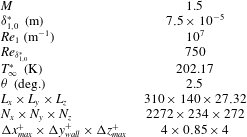
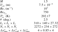
A laminar boundary layer on a flat plate at an inflow Mach number $M=1.5$ , free-stream temperature $T_{\infty }^{\ast }=202.17~\text{K}$ and unit Reynolds number $Re_{1}=10^{7}~\text{m}^{-1}$ is impinged with an oblique shock wave. The inflow conditions are the same as in the experiments carried out at the Institute of Theoretical and Applied Mechanics (ITAM) in Novosibirsk, Russia, as part of the European TFAST Project (http://www.tfast.eu). For the present DNS study, the interaction is taken to be close to the leading edge and a Reynolds number based on the displacement thickness at the computational domain inlet is selected to be $Re_{{\it\delta}_{1,0}^{\ast }}=750$ , where ${\it\delta}_{1,0}^{\ast }=7.5\times 10^{-5}~\text{m}$ . The non-dimensional integration time step is ${\rm\Delta}t=0.04$ and the wall temperature is $T_{w}^{\ast }=279.20~\text{K}$ . An oblique shock wave, generated with a wedge angle ${\it\theta}=2.5^{\circ }$ , is introduced at the upper boundary of the computational domain at $Re_{x_{sw}}=0.95\times 10^{5}$ and impinges onto the boundary layer at $Re_{x_{imp}}=1.95\times 10^{5}$ , as represented schematically in figure 1. A 2D base flow is obtained for a numerical domain that extends far enough in the streamwise direction to contain the whole separation bubble and high enough in the wall-normal direction to avoid any potential reflections of the shock wave from the top boundary impinging on the boundary layer. The 2D base flow is then extruded in the spanwise direction over a width equal to the spanwise wavelength ( ${\it\lambda}_{z}$ ) of the unstable 3D mode within the separation bubble (this will be shown in detail in the next section). The domain size, normalized with the inlet displacement thickness, is therefore selected to be $(L_{x},L_{y},L_{z})=(310,140,27.32)$ , giving a streamwise range of Reynolds number $Re_{x}=(0.80{-}3.13)\times 10^{5}$ . The grid size is chosen in order to resolve transition and turbulence at the back of the bubble. For this reason, the grid is stretched in the streamwise and wall-normal directions to have more grid points clustered downstream of the impingement location and near the wall, respectively. The number of points in the streamwise, wall-normal and spanwise directions are chosen as $(N_{x},N_{y},N_{z})=(2272,234,272)$ , corresponding to grid sizes $({\rm\Delta}x_{max}^{+},{\rm\Delta}y_{wall}^{+},{\rm\Delta}z_{max}^{+})=(4,0.85,4)$ (where wall units are denoted by superscript $+$ and defined as $x_{i}^{+}=x_{i}u_{{\it\tau}}/{\it\nu}$ ). The numerical set-up is summarized in table 1. The fully time-converged 2D-DNS base flow is obtained, and density contours (a), skin friction (b) and wall-pressure (c) distributions are plotted in figure 2. The laminar boundary-layer skin friction solution by Eckert (Reference Eckert1955) is also plotted in figure 2(b). A long steady separation bubble is formed for an adverse pressure gradient of $p_{d}/p_{\infty }=1.28$ (where $p_{d}$ indicates the pressure downstream of the reflected shock) and captured entirely within the numerical domain. Downstream of the interaction the flow does not fully recover to an equilibrium laminar boundary-layer solution within the domain.

Figure 1.

Schematic representation of the numerical set-up. The shock generator plate with wedge angle ${\it\theta}$ introduces a shock wave from the top boundary at $x_{sw}$ that impinges onto the boundary layer at $x_{imp}$ . The displacement thickness at the numerical inlet ${\it\delta}_{1,0}^{\ast }$ is used as a characteristic length. Free-stream and downstream regions are indicated with the subscripts $\infty$ and $d$ , respectively.

Table 1.

Inflow conditions and numerical set-up of the 3D SWBLI case.

Figure 2.

Two-dimensional steady base flow description: (a) density contours, (b) skin friction and (c) normalized wall-pressure distributions. The laminar boundary-layer skin friction result from Eckert (Reference Eckert1955) is also plotted (dashed line).

2.3 Transition tripping: modal forcing technique

To obtain transition to turbulence, the 3D steady base flow is forced by adding ‘modal’ disturbances, whose shape is defined by eigenfunctions corresponding to specifically selected eigenvalues. For the conservative variables vector $\boldsymbol{q}$ , the forcing at the inlet is $\boldsymbol{q}_{0}=\bar{\boldsymbol{q}}_{0}+\boldsymbol{q}_{0}^{\prime }$ , where $\bar{\boldsymbol{q}}_{0}$ is the steady base flow and $\boldsymbol{q}_{0}^{\prime }$ are the disturbances, which can be described as

(2.10) $$\begin{eqnarray}\boldsymbol{q}_{0}^{\prime }(y,z,t)=\boldsymbol{q}^{\prime }(x=0,y,z,t)=A_{o}\,\text{Re}\{\hat{\boldsymbol{q}}(y)\exp [\text{i}({\it\alpha}x\pm {\it\beta}z-{\it\omega}t)]\},\end{eqnarray}$$

where $A_{o}$ is the amplitude of the disturbances, $\hat{\boldsymbol{q}}(y)$ are the eigenfunctions calculated with local LST, ${\it\alpha}$ is the streamwise wavenumber, ${\it\beta}$ is the spanwise wavenumber and ${\it\omega}$ is the (single) frequency. The modal forcing is applied as a prescribed time-dependent inlet boundary condition. No-slip and isothermal (with the temperature equal to the laminar adiabatic wall temperature) conditions are enforced at the wall, an integrated characteristic method is applied at the top boundary and a standard characteristic boundary condition is used at the outflow. Periodic boundary conditions are applied in the spanwise direction. The instability of a boundary layer changes in the presence of a separation bubble and different modes can become unstable compared to a ZPG case. Temporal stability maps are calculated both at the inlet at $Re_{x}=0.80\times 10^{5}$ (virtually for a ZPG boundary layer) and within the separation bubble at $Re_{x}=1.78\times 10^{5}$ and respectively presented in figure 3(a,b), where the imaginary part of the frequency ${\it\omega}_{i}$ is plotted for different combinations of ${\it\alpha}$ and ${\it\beta}$ . For both cases, the unstable mode selected is a 3D wave that corresponds to ${\it\alpha}=0.240$ , ${\it\beta}=0.140$ with ${\it\omega}_{r}=0.123$ for the ZPG case and to ${\it\alpha}=0.200$ , ${\it\beta}=0.230$ and ${\it\omega}_{r}=0.101$ within the separation bubble. As expected, the separated boundary layer becomes more unstable and the imaginary part of ${\it\omega}$ increases by two orders of magnitude (from 0.00053 to 0.02546). Some differences might arise if the stability analysis was repeated using a spatial approach, especially in the presence of a separated boundary layer. Confirming the link between temporal and spatial unstable waves (Gaster Reference Gaster1962), for the ZPG boundary layer no differences are observed, while for the separated case the Gaster-transformed growth rate of the most unstable mode from spatial theory is within 15 % of that obtained from temporal theory. The scope of the present analysis is to find a combination of modes that effectively triggers transition to turbulence. Thus, the 3D unstable mode identified within the separation bubble is chosen and spatial linear stability is used to calculate the corresponding eigenfunctions at the inflow. An oblique mode breakdown has been shown to be the predominant transition scenario for low supersonic boundary layers (Fasel, Thumm & Bestek Reference Fasel, Thumm, Bestek, Kral and Zang1993; Sandham & Adams Reference Sandham and Adams1993; Sandham, Adams & Kleiser Reference Sandham, Adams and Kleiser1995; Mayer, Von Terzi & Fasel Reference Mayer, Von Terzi and Fasel2011); therefore a pair of oblique modes with $({\it\omega},{\it\beta})=(0.101,\pm 0.230)$ is selected to force the separated boundary layer. This information on the selected unstable mode is also used to set the width of the numerical domain to be equal to one wavelength of the identified 3D wave, therefore $L_{z}={\it\lambda}_{z}=2{\rm\pi}/{\it\beta}=27.32$ .

Figure 3.

Temporal stability maps for (a) a ZPG boundary layer at $Re_{x}=0.80\times 10^{5}$ and (b) within the separation bubble at $Re_{x}=1.78\times 10^{5}$ . Contours of the imaginary part of the frequency/eigenvalue ${\it\omega}_{i}$ for combinations of the streamwise ${\it\alpha}$ and spanwise ${\it\beta}$ wavenumbers.

3.1 Base flow selection

The same 2D base flow for a wedge angle ${\it\theta}=2.5^{\circ }$ presented in § 2.2 is here considered for the comparison between DNS and linear stability methods. For this case, the separation bubble is relatively large and, since the analysis is aimed to investigate different non-parallel effect intensities, a weaker shock at ${\it\theta}=1.3^{\circ }$ is also considered and a ‘marginal separation’ is obtained. The Reynolds number at the inlet is kept fixed and, in order to have the same impingement location of the shock wave on the boundary layer, the shock is introduced slightly earlier at $Re_{x_{sw}}=0.91\times 10^{5}$ for the marginal separation case. Since only a linear investigation is intended, the grid resolution is coarsened with respect to the one presented in § 2.2 and selected to be $(N_{x},N_{y})=(1000,200)$ . The 2D base flow is considered to be grid-independent when the difference in the separation bubble length $L_{SB}$ for different resolutions is less than $1\,\%$ , and a grid resolution study is presented in table 2. The 3D base flow is constructed by extruding the 2D base flow in the spanwise direction. A domain size $(L_{x},L_{y},L_{z})=(310,140,{\it\lambda}_{z})$ is selected for the large separation case and, for simplicity, also used for the marginal separation case. The domain width is fixed to be one spanwise wavelength ( ${\it\lambda}_{z}$ ) of the 3D mode selected and will be specified case by case. For small-amplitude (linear) problems $16$ grid points in the spanwise direction are sufficient as only one wave needs to be resolved. For validation and comparison purposes, a ZPG boundary layer is also analysed.

Figure 4.

Skin friction (a) and wall-pressure (b) distributions for the ZPG (dashed line), marginal separation (dash-dotted line) and large separation (solid line) cases.

Table 2.

Grid resolution study for the marginal ( ${\it\theta}=1.3^{\circ }$ ) and large ( ${\it\theta}=2.5^{\circ }$ ) separation cases.

For each case, the simulations are run long enough in time to obtain a fully converged solution. It is possible to appreciate the differences in bubble size and pressure gradient for the investigated shock strengths by analysing the skin friction and wall-pressure distributions for the ZPG (dashed line), marginal separation (dash-dotted line) and large separation (solid line) cases reported in figures 4(a) and 4(b), respectively.

To verify the applicability of the stability tools to these separated flows, it is necessary to check whether the boundary layer is convectively unstable. The reverse flow magnitude within the separation bubble can be considered as an indicator. The maximum reverse flow magnitude for each streamwise location is plotted (dashed line) in the region around the separation bubble for both marginal and large separation cases in figure 5(a,b), where separation (S) and reattachment (R) points are also indicated. The streamwise velocity profiles at different locations are also plotted to show the regions where reverse flow exists (black solid lines). The maximum reverse flow magnitude is 0.06 % for the marginal separation case and 6 % for the large separation case. Following the criterion given by Alam & Sandham (Reference Alam and Sandham2000) and Rist (Reference Rist2004), for which separated boundary layers are absolutely unstable when the maximum reverse flow magnitudes are larger than 20 %, the boundary layers under investigation can be considered almost certainly convectively unstable.

Figure 5.

Marginal (a) and large (b) separation cases: streamwise distribution of the maximum reverse flow magnitude (dashed line) and streamwise velocity profiles (black solid lines) in the region around the separation bubble. Separation and reattachment points are indicated with (S) and (R), respectively.

These DNS base flows are used for the LST and LPSE analysis and are interpolated in the wall-normal direction over $250$ grid points using the mapping Chebyshev collocation method. For the local LST analysis, the streamwise evolution of the streamwise wavenumber is obtained by repeating the analysis at different $x$ locations independently. For the non-local analysis, the streamwise derivatives of the pressure terms are retained and the method is stabilized by choosing a sufficiently large marching integration step ${\rm\Delta}x_{PSE}$ . The sensitivity of the LPSE solution to the marching integration step is analysed by using ${\rm\Delta}x_{PSE}=3{\it\delta}_{1,0}^{\ast },6{\it\delta}_{1,0}^{\ast },12{\it\delta}_{1,0}^{\ast }$ and $24{\it\delta}_{1,0}^{\ast }$ .

While the $n$ -factor from the stability analysis methods is calculated as

(3.1) $$\begin{eqnarray}n_{LST/LPSE}(x)=-\int _{x=0}^{x}{\it\alpha}_{i}\,\text{d}\tilde{x}=\ln \left(\frac{A}{A_{x=0}}\right),\end{eqnarray}$$

the DNS $n$ -factor is defined to be

(3.2) $$\begin{eqnarray}n_{DNS}(x)=\ln \left[\frac{A_{DNS}(x)}{A_{DNS}(x=0)}\right],\end{eqnarray}$$

where

(3.3) $$\begin{eqnarray}A_{DNS}=\sqrt{\int _{0}^{y_{e}}(|\hat{{\it\rho}}|^{2}+|\hat{u} |^{2}+|\hat{v}|^{2}+|{\hat{w}}|^{2}+|\hat{T}|^{2})\,\text{d}y}.\end{eqnarray}$$

The integration is evaluated between the wall and the edge of the boundary layer ( $y_{e}$ ) using fast Fourier transforms (FFTs) of time series of the primitive variable flow quantities (indicated with the hat symbol). The time series are accumulated over four periods of the forced mode.

3.2 ZPG boundary layer

Modal disturbances, as described in § 2.3, are applied at the inlet to force the ZPG boundary layer, and the temporal stability map reported in figure 3(a) is used to select the modes of interest. A 2D wave ( ${\it\alpha}=0.240$ , ${\it\beta}=0.00$ and ${\it\omega}=0.124$ ) and a 3D one ( ${\it\alpha}=0.240$ , ${\it\beta}=0.140$ and ${\it\omega}=0.123$ ) are chosen and the domain spanwise width is therefore fixed to $L_{z}={\it\lambda}_{z}=2{\rm\pi}/{\it\beta}=44.9$ .

Figure 6.

Streamwise evolution of the maximum $n$ -factor for a 2D (a) and 3D (b) mode. Comparison between DNS (circles), LST (dashed line) and LPSE (solid line with error bars).

Figure 6 shows the streamwise evolution of the maximum $n$ -factors for the 2D (a) and the 3D (b) waves calculated from DNS (circles), LST (dashed line) and LPSE (solid line with error bars showing the standard deviation of the variations due to the integration step size sensitivity). The modes selected are unstable at the inlet and initially grow, but they become stable and decay further downstream. While it is clear that the LST suffers because of the non-parallelism of the base flow, very good agreement is obtained between DNS and LPSE for both regions of the flow when the disturbances grow and decay.

3.3 Shock-induced separated boundary layer

The same 2D and 3D waves used for the validation of the LPSE tool on the ZPG non-parallel boundary layer are selected to force the marginal and large separation cases and modal forcing is applied at the inlet. With ${\it\beta}=0.14$ , the spanwise width of the numerical domain is again $L_{z}=44.9$ . Similarly to the previous case, the streamwise evolution of the $n$ -factors for the 2D and 3D waves calculated from DNS (circles) are compared with the predictions of LST (dashed line) and LPSE (solid line) and reported in figure 7(a,b) for the marginal separation case, and in figure 7(c,d) for the large separation case. The effect of the integration step size on the LPSE growth rates is represented by the error bars, which indicate the mean standard deviation. It is interesting to see that, for both 2D and 3D waves, the LPSE tool is able to accurately reproduce the disturbance growth rates when the boundary layer is marginally separated. When the shock strength increases and a large separation occurs, the LPSE tool agrees very well with the DNS for the 2D wave but is less accurate when a 3D wave is considered. In this case, the errors accumulate in the streamwise direction and lead to a disagreement in the second half of the bubble. Differently from what was observed by Hein (Reference Hein2005), the growth at the separation point is still well predicted and deviates only when the reverse flow is stronger. On the other hand, LST suffers due to the non-parallelism of the base flows; nevertheless the disturbance growth rates do not differ excessively from DNS or LPSE. For example, if we consider the large separation case, where the growth rates are high, the maximum relative error between DNS and LST is only approximately 11 %. For the marginal separation case the relative error is bigger, but only because small growth of the disturbances is observed.

Figure 7.

Streamwise evolution of the $n$ -factor for 2D (a,c) and 3D (b,d) modes for the marginal separation (a,b) and large separation (c,d) cases. Comparison between DNS (circles), LST (dashed line) and LPSE (black line with error bars).

As highlighted in § 2.3, it is important to note that the previously selected waves are unstable at the inlet and that, in the presence of separation, different modes become unstable. The comparison between DNS, LST and LPSE is therefore repeated for the large separation case by considering a 2D wave that corresponds to ${\it\alpha}=0.200$ , ${\it\beta}=0.000$ and ${\it\omega}=0.098$ and a 3D wave with ${\it\alpha}=0.200$ , ${\it\beta}=0.230$ and ${\it\omega}=0.101$ . Thus, the spanwise width of the numerical domain is now $L_{z}=27.3$ . In figure 8(a,b) the streamwise evolutions of the 2D and 3D waves in the separated boundary layer are plotted for DNS (circles), LST (dashed line) and LPSE (solid line with error bars). It is important to note that this set of unstable modes within the separation bubble reaches higher $n$ -factors with respect to the set of unstable modes at the inlet, confirming that the separation bubble acts like a spatial filter–amplifier. It appears again that the LPSE tool struggles to represent the growth of the 3D wave in the streamwise direction when strong reverse flow is present. In this case, the LPSE calculations have been performed by neglecting the $\partial p/\partial x$ terms in order to stabilize the code, and a higher sensitivity to the integration step size is found as shown by the increase in the error bars. Similarly to Pagella et al. (Reference Pagella, Babucke and Rist2004), LST still does not match DNS but is not excessively inaccurate, with a maximum relative error of 15 %.

Figure 8.

Streamwise evolution of the $n$ -factor for a 2D (a) and 3D (b) mode for the large separation bubble case and modes calculated at $Re_{x}=1.31\times 10^{5}$ . Comparison between DNS (circles), LST (dashed line) and LPSE (solid line with error bars).

Figure 9.

Time- and span-averaged (black solid line) and instantaneous span-averaged (light grey solid line) skin friction distributions of the 3D forced SWBLI configuration. Laminar (Eckert Reference Eckert1955) (black dashed line), turbulent (Young Reference Young1989) (black dash-dotted line) and 2D base flow (dark grey solid line) skin friction distributions are also plotted for reference.

4.1 Breakdown to turbulence

Transition happens in the vicinity of the reattachment point and reduces significantly the separation length as shown by the time- and span-averaged skin friction distributions in figure 9 (black solid line) with respect to the 2D base flow (dark grey solid line). The laminar (black dashed line) and turbulent (black dash-dotted line) boundary-layer solutions by Eckert (Reference Eckert1955) and Young (Reference Young1989), respectively, are also plotted. An instantaneous span-averaged skin friction distribution at the non-dimensional time $t=55\,000$ (light grey solid line) is also reported to show the strong unsteady character of the flow near the reattachment point and further downstream. Isosurfaces of the instantaneous wall-normal vorticity are plotted for the levels ${\it\omega}_{y}=+0.08$ (red) and ${\it\omega}_{y}=-0.08$ (black) and coloured with the streamwise velocity in figure 10(a) to illustrate the breakdown scenario. It is also interesting to see from figure 10(b), where contours of the streamwise vorticity ${\it\omega}_{x}$ in $z$ – $y$ planes are plotted at different streamwise locations, that the oblique-mode transition causes the appearance of strong streamwise vortices (see the $z$ – $y$ plane at $Re_{x}\approx 2.32\times 10^{5}$ ) that develop downstream and break down to turbulence. The modes selected to force the separated boundary layer affect the breakdown to turbulence and the separation bubble size. In this case, the symmetric nature of the forcing imposed at the inlet causes the breakdown also to be symmetric in the whole domain except for a small region towards the outlet. Similarly to what was obtained numerically by Nikitin (Reference Nikitin2008) and later experimentally by Borodulin, Kachanov & Roschektayev (Reference Borodulin, Kachanov and Roschektayev2011), the turbulence obtained at the back of the bubble is essentially deterministic turbulence that is reproducible over a period of the forcing frequency. An analogous phenomenon was also seen in the DNS transition study by Sandham & Kleiser (Reference Sandham and Kleiser1992) for a plane channel flow, for which the shear-layer roll-up into discrete vortices was happening while the imposed initial spanwise symmetry was still preserved, defining the process as deterministic rather than triggered by the growth of the random background numerical noise.

Figure 11.

Amplitude of the time-transformed Fourier modes of the span-averaged wall-pressure fluctuations, $|\mathscr{F}_{t}(p_{w}-\bar{p}_{w})|$ , calculated at the streamwise locations (a)  $Re_{x}=1.29\times 10^{5}$ , (b)  $Re_{x}=1.74\times 10^{5}$ , (c)  $Re_{x}=2.15\times 10^{5}$ and (d)  $Re_{x}=3.09\times 10^{5}$ .

4.2 Spectral analysis

A spectral analysis is carried out for wall-pressure time series collected over a time period long enough to ensure that the minimum frequency of the spectra is two orders of magnitude smaller than the forcing frequency ( $f=0.016$ ). The time series are recorded over the whole wall plane with $16$ samples for each period. The recorded signals are broken into three segments with 50 % overlapping (Welch Reference Welch1967; Hu, Morfey & Sandham Reference Hu, Morfey and Sandham2006). A Strouhal number, $St$ , based on the time- and span-averaged separation bubble length $L_{SB}=67.8$ (see figure 9), is used to plot the amplitude of the Fourier transform in time of the wall-pressure fluctuations, $|\mathscr{F}_{t}(p_{w}-\bar{p}_{w})|$ ; $St$ is linked to the dimensionless frequency as $St=L_{SB}\,f$ . The spectral analysis is performed for each $x$ and $z$ location on the wall. However, the spectra are found to be unaffected by the spanwise position, except for the $z$ locations corresponding to the zero node of the spanwise modulation applied to the forcing, i.e. at $z=L_{z}/4$ and $3L_{z}/4$ . Thus, the wall-pressure time series at each streamwise location can be span-averaged before the calculation of the spectra. Figure 11 shows the $|\mathscr{F}_{t}(p_{w}-\bar{p}_{w})|$ frequency distribution at different streamwise locations moving from the inlet towards the outlet, chosen as (a) upstream of the separation point and at the beginning of the interaction region at $Re_{x}=1.29\times 10^{5}$ , (b) at the separation point $Re_{x}=1.74\times 10^{5}$ , (c) at the reattachment point $Re_{x}=2.15\times 10^{5}$ and (d) in the turbulent region at $Re_{x}=3.09\times 10^{5}$ . Each location shows a narrow peak at $St=1.091$ that corresponds to the applied forcing. This causes the appearance of higher harmonics, visible as narrow peaks at multiples of the forcing Strouhal number. It is interesting to see from figure 11 that a low-frequency broadband peak appears. The low-frequency unsteadiness starts to become energetically significant at the beginning of the interaction region (figure 11 b). The deterministic components associated with the applied forcing cause the rise of the unforced/non-deterministic modes and, moving downstream towards the turbulent region (figure 11 d), the energy content at high frequencies increases, the spectrum flattens out and only the forcing frequency and its harmonics can be distinguished. The spatial extent of the low-frequency broadband peak can be more clearly seen by plotting the contours of the frequency-weighted wall-pressure Fourier modes $f\,|\mathscr{F}_{t}(p_{w}-\bar{p}_{w})|$ normalized with its maximum in frequency for each streamwise location as a function of the streamwise location and Strouhal number in figure 12. A broadband peak at frequencies around $St=0.04$ is localized just upstream of the separation point, marked by the vertical black dashed line on the figure. This low-frequency broadband peak is located at a Strouhal number that is comparable to the low-frequency unsteadiness found for the turbulent interactions (Dussauge, Dupont & Debiéve Reference Dussauge, Dupont and Debiéve2006; Touber & Sandham Reference Touber and Sandham2009), suggesting a close analogy between the laminar and turbulent cases. However, it is important to note that the mechanism producing the low-frequency unsteadiness in the laminar case yields only very low amplitude levels, whereas in the turbulent case both the background disturbances and the low-frequency response are large.

From the results shown in figures 11 and 12, it is now possible to identify the origin of the low-frequency unsteadiness in the breakdown of deterministic turbulence, which creates a broadband white noise spectrum (zero slope in figure 11 d) downstream of the reattachment. Similarly to the 2D interaction presented in Sansica et al. (Reference Sansica, Sandham and Hu2014), where the low frequency was explicitly forced with white noise, these disturbances can travel upstream in the subsonic region of the boundary layer and the low-frequency unsteadiness becomes relatively more significant just upstream of the separation point. The presence of upstream-travelling disturbances is demonstrated in figure 13, where the Strouhal number/streamwise wavenumber spectrum calculated in the streamwise range $Re_{x}=(1.00{-}2.88)\times 10^{5}$ is presented. For positive values of ${\it\alpha}$ , the amplitude of the double Fourier transform in space and time of the span-averaged wall-pressure fluctuations shows the deterministic downstream-travelling component of the forcing at $({\it\alpha},St)=(0.200,1.091)$ and its first harmonic. The upstream-travelling disturbances are visible for negative values of ${\it\alpha}$ , where a straight line with constant phase speed $c_{ph}\approx -0.6$ stretches from low to high frequencies. Considering the near-zero velocity of the flow within the separation bubble, this value is very close to the speed of an upstream-travelling acoustic wave at $M=1.5$ , suggesting the acoustic nature of the waves responsible for the appearance of the low-frequency unsteadiness.

Figure 12.

Contours of $f\,|\mathscr{F}_{t}(p_{w}-\bar{p}_{w})|$ normalized with its maximum in frequency for each streamwise location as a function of the streamwise location and Strouhal number. Contour levels are set on a logarithmic scale between $10^{-11}$ and $10^{-7}$ . The vertical black dashed line indicates the streamwise location of the separation point.

Figure 13.

Strouhal number/streamwise wavenumber spectrum. The amplitude of the double Fourier transform in space and time of the span-averaged wall-pressure fluctuations shows the deterministic downstream-travelling components and upstream-travelling waves. The black dashed line indicates zero values of ${\it\alpha}$ .

4.2.1 Low-frequency unsteadiness sensitivity

The low-frequency energy content that arises from the broadband white noise created by the breakdown of the deterministic turbulence is at very low amplitudes and might be sensitive to the numerical details of the simulation. Here, grid resolution and domain size (to study the influence of outflow and free-stream boundaries) are considered as the two major parameters that can affect the response of the separated region.

A grid resolution study is carried out on the 3D base flow configuration for a grid that was coarsened by a factor of 2 in all three directions. The time- and span-averaged skin friction distributions for the coarse and fine grid cases are in good agreement and the fine grid is therefore considered suitable for the present study (Sansica Reference Sansica2015). This base flow is used here to repeat the spectral analysis previously presented, and the amplitude of the Fourier transform in time of the wall-pressure fluctuations, $|\mathscr{F}_{t}(p_{w}-\bar{p}_{w})|$ , is reported for different $x$ locations in figure 14 (black line). Using the same resolution, an additional simulation was performed with the domain increased in height by $20{\it\delta}_{1,0}^{\ast }$ and in length by $30{\it\delta}_{1,0}^{\ast }$ further downstream. The spectral analysis relative to this enlarged numerical domain is also presented in figure 14 (light grey line).

Figure 14.

Grid resolution and domain size sensitivity. Amplitude of the Fourier transform in time of the wall-pressure fluctuations, $|\mathscr{F}_{t}(p_{w}-\bar{p}_{w})|$ , calculated from span-averaged wall-pressure time series at the streamwise locations (a)  $Re_{x}=1.29\times 10^{5}$ , (b)  $Re_{x}=1.74\times 10^{5}$ , (c)  $Re_{x}=2.15\times 10^{5}$ and (d)  $Re_{x}=3.09\times 10^{5}$ . Fine grid (dark grey line; the lowest curve in each case), coarse grid (black line) and coarse grid with enlarged domain (light grey line).

The low-frequency response of the separation bubble still exists and arises from the broadband numerical white noise. However, it is interesting to see the sensitivity of the energy content for both low-frequency and non-deterministic parts of the spectra, which increase both for the coarse grid and coarse grid enlarged domain cases with respect to the fine grid simulation (dark grey line). This is because the numerical background noise generated by the coarse grid is higher, as is visible upstream of the separation point (figure 14 a) where the non-deterministic part of the spectra at high frequencies reaches an amplitude approximately three orders of magnitude larger than the fine grid case. However, the energy of the low-frequency broadband peak only increases by one order of magnitude. This observation again links the low-frequency unsteadiness with the broadband white noise spectrum created by the breakdown to turbulence that also increases by approximately one order of magnitude (figure 14 d). This is also true for the coarse grid enlarged domain case, where, despite some small differences in the amplitude of the non-deterministic white noise component due to the influence of the outflow boundary, the energy level of the low frequency is practically unchanged. It could be argued that the low frequency could be reduced by further refining the numerical grid, but the existence of broadband white noise will always be present in real-world applications (i.e. noise generated by wind tunnel walls, free-stream turbulence, etc.) and contribute to the appearance of the unsteadiness.

This analysis shows that different types of broadband perturbations can produce the low-frequency unsteadiness, as already shown in Sansica et al. (Reference Sansica, Sandham and Hu2014). While in that case an energetically higher low-frequency response was obtained by explicitly forcing the low-frequency unsteadiness with random white noise, here the unsteadiness is indirectly created by the breakdown of the deterministic turbulence.