2.1 Governing equations

The simulations presented here are based on the compressible Navier–Stokes equations:

(2.1) $$\begin{eqnarray}\displaystyle & \displaystyle \frac{\unicode[STIX]{x2202}\unicode[STIX]{x1D70C}}{\unicode[STIX]{x2202}t}+\unicode[STIX]{x1D735}\boldsymbol{\cdot }(\unicode[STIX]{x1D70C}\boldsymbol{u})=0, & \displaystyle\end{eqnarray}$$

(2.2) $$\begin{eqnarray}\displaystyle & \displaystyle \frac{\unicode[STIX]{x2202}}{\unicode[STIX]{x2202}t}(\unicode[STIX]{x1D70C}\boldsymbol{u})+\unicode[STIX]{x1D735}\boldsymbol{\cdot }(\unicode[STIX]{x1D70C}\boldsymbol{u}\boldsymbol{u})=-\unicode[STIX]{x1D735}p+\unicode[STIX]{x1D735}\boldsymbol{\cdot }\text{}\underline{\unicode[STIX]{x1D749}}+\unicode[STIX]{x1D70C}\boldsymbol{f}+\boldsymbol{S}, & \displaystyle\end{eqnarray}$$

(2.3) $$\begin{eqnarray}\displaystyle & \displaystyle \frac{\unicode[STIX]{x2202}}{\unicode[STIX]{x2202}t}(\unicode[STIX]{x1D70C}e)+\unicode[STIX]{x1D735}\boldsymbol{\cdot }(\unicode[STIX]{x1D70C}e\boldsymbol{u})=-p\unicode[STIX]{x1D735}\boldsymbol{\cdot }\boldsymbol{u}+\unicode[STIX]{x1D735}\boldsymbol{\cdot }(\unicode[STIX]{x1D705}\unicode[STIX]{x1D735}T)+\text{}\underline{\unicode[STIX]{x1D749}}\boldsymbol{\cdot }\unicode[STIX]{x1D735}\boldsymbol{u}+S_{e}, & \displaystyle\end{eqnarray}$$

where $\unicode[STIX]{x1D70C}$ is density, $\boldsymbol{u}$ is the velocity vector, $p$ is pressure, $\text{}\underline{\unicode[STIX]{x1D749}}$ is the stress tensor for a Newtonian fluid given by $\unicode[STIX]{x1D70F}_{ij}=\unicode[STIX]{x1D707}(\unicode[STIX]{x2202}u_{i}/\unicode[STIX]{x2202}x_{j}+\unicode[STIX]{x2202}u_{j}/\unicode[STIX]{x2202}x_{i}-(2/3)\unicode[STIX]{x1D6FF}_{ij}\unicode[STIX]{x2202}u_{k}/\unicode[STIX]{x2202}x_{k})$ with zero bulk viscosity, $\boldsymbol{f}$ is the body force vector used to generate turbulence, $\boldsymbol{S}$ is a sponge vector, $e$ is internal energy, $\unicode[STIX]{x1D705}$ is thermal conductivity and $T$ is temperature. The viscosity follows a power law with temperature as $\unicode[STIX]{x1D707}=\unicode[STIX]{x1D707}_{0}(T/T_{0})^{0.75}$ ( $\unicode[STIX]{x1D707}_{0}$ and $T_{0}$ are reference values) and the Prandtl number is assumed to be constant at $Pr=0.72$ . To close the system of equations, an ideal gas is assumed which follows the equation of state $p=\unicode[STIX]{x1D70C}RT$ with $R$ being the gas constant of the fluid. The ratio of specific heats is $\unicode[STIX]{x1D6FE}=1.4$ . As in virtually all previous studies (§ 1), the flow is assumed to be a continuum which is justified at the conditions presented here (Moser Reference Moser2006). As in Donzis & Jagannathan (Reference Donzis and Jagannathan2013) and Jagannathan & Donzis (Reference Jagannathan and Donzis2016), discretization of spatial derivatives is performed with tenth-order compact schemes whose numerical and computational advantages are well known (Lele Reference Lele1992a ).

2.2 Numerical methods

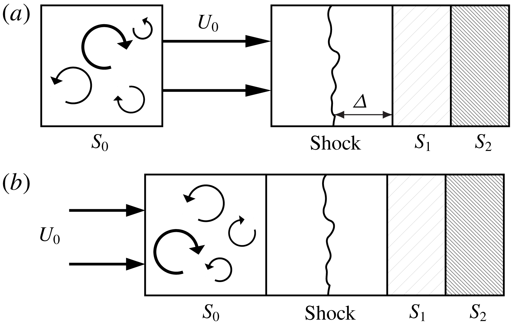
In order to assess the generality of the theoretical results presented here, two approaches are used to generate turbulence which yield isotropic and anisotropic fluctuations. The two methods used the same code and adopt the same forcing. The difference between the two approaches lies on where the forcing is applied ( $S_{0}$ ) as is seen in the schematic diagrams given in figure 1. This forcing consists of an additional body force in the momentum equation which is stochastic and applied at large scales. This force is constructed using integrated Ornstein–Uhlenbeck processes with finite-time correlation in Fourier space. In physical space, the forcing can be written as

(2.4) $$\begin{eqnarray}\boldsymbol{f}=\mathop{\sum }_{|k|<k_{F}}\hat{\boldsymbol{f}}_{\bot }(\boldsymbol{k})\text{e}^{-\text{i}\boldsymbol{k}\boldsymbol{\cdot }\boldsymbol{x}},\end{eqnarray}$$

where $\hat{\boldsymbol{f}}_{\bot }(\boldsymbol{k})=(\boldsymbol{I}-\boldsymbol{k}\boldsymbol{k}/k^{2})\boldsymbol{\cdot }\hat{\boldsymbol{f}}$ is the projection of the mode at wavenumber $\boldsymbol{k}$ onto a plane perpendicular to the wave vector itself. This guarantees that the stirring mechanism is, by construction, solenoidal. The forcing parameters are chosen to achieve a given $R_{\unicode[STIX]{x1D706}}$ and $M_{t}$ and, at the same time, yield integral length scales which are a fraction of the domain size. Further details of the forcing and statistics of the resulting turbulence fields are described in Donzis & Jagannathan (Reference Donzis and Jagannathan2013) and Jagannathan & Donzis (Reference Jagannathan and Donzis2016).

Figure 1.

A schematic of the shock interacting with (a) isotropic turbulence and (b) anisotropic turbulence in the computational domains.

The two approaches that result in isotropic and anisotropic turbulence, respectively, are now described.

Isotropic turbulence (IT). In this procedure a separate simulation of isotropic turbulence in a triply periodic domain ( $S_{0}$ ) is conducted (figure 1 a). Once in stationary state, the turbulence is convected through the inlet using Taylor hypothesis at a velocity $U_{0}$ which corresponds to a mean Mach number, $M$ . A similar procedure has been used before in the literature with forced (e.g. Ryu & Livescu Reference Ryu and Livescu2014) and decaying turbulence (e.g. Mahesh et al. Reference Mahesh, Lele and Moin1997; Larsson & Lele Reference Larsson and Lele2009) though forcing details are somewhat different.

Spatially developing turbulence (SDT). In this approach, turbulence is generated upstream of the shock in $S_{0}$ in a single simulation as it is convected at $U_{0}$ (figure 1 b). The domain is longer in the streamwise direction than that for the isotropic approach above. The interaction between the fluctuations and the mean flow in $S_{0}$ , results in unequal production rates in the streamwise and transverse components (Taylor Reference Taylor1935). The result is a slightly anisotropic flow with a streamwise component of the velocity variance larger than transverse components. Such flow is closer to grid-generated turbulence in wind tunnels where anisotropy in the turbulence has been consistently observed (Grant & Nisbet Reference Grant and Nisbet1957; Mohamed & Larue Reference Mohamed and Larue1990).

To sustain a statistically stationary shock at a prescribed location in the domain it is necessary to impose a relatively high pressure downstream of the shock which is done here using a sponge region ( $S_{1}$ in figure 1). For a shock in a uniform flow, the appropriate pressure jump is given by standard Rankine–Hugoniot relations. However, the interaction of turbulent fluctuations with the normal shock produces a well-known slow drift of the shock (Lee et al. Reference Lee, Lele and Moin1993; Larsson et al. Reference Larsson, Bermejo-Moreno and Lele2013; Ryu & Livescu Reference Ryu and Livescu2014) which is due to the changes in post-shock pressure when upstream fluctuations are present. In a typical STI simulation the back pressure is commonly adjusted in a trial-and-error fashion. Our analytical results below, instead, provide the explicit dependence of pressure jumps on characteristics of the upstream turbulence.

In addition, care has to be taken to avoid boundary reflections as the flow becomes subsonic downstream of the normal shock. Thus, we use a second sponge ( $S_{2}$ in figure 1) between $S_{1}$ and the outlet. In this region the flow is smoothly accelerated to supersonic speeds such that no characteristic travels upstream from the outlet avoiding potential effects from outflow boundary conditions. This approach has been used and tested in previous studies (Freund Reference Freund1997; Ryu & Livescu Reference Ryu and Livescu2014). In both sponge regions $S_{1}$ and $S_{2}$ we include a body force of the following form:

(2.5) $$\begin{eqnarray}S_{q}=A\langle q\rangle \frac{(x-x_{s1})^{n_{1}}(x-x_{s2})^{n_{2}}}{l_{s}^{n1+n2+1}}(q_{ref}-q),\end{eqnarray}$$

where $A$ is a constant, $\langle \cdot \rangle$ represents an average over the sponge region, $x_{s1}$ and $x_{s2}$ are the beginning and the end points of a sponge, $l_{s}$ is the length of a sponge, $n_{1}$ and $n_{2}$ are constant exponents and subscript ‘ref’ stands for the specified value that a variable inside the sponge converges to (pressure in $S_{1}$ and streamwise velocity in  $S_{2}$ ).

Figure 2.

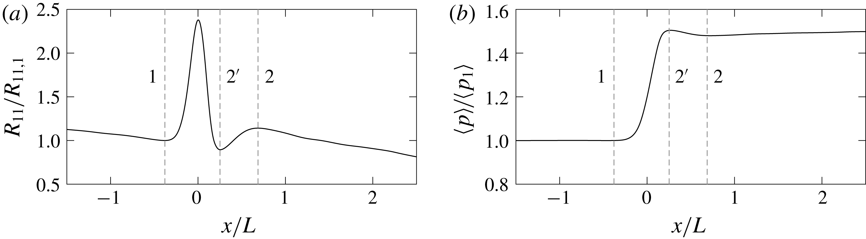
Typical streamwise distribution of (a) Reynolds stress $R_{11}$ and (b) pressure, both normalized by their upstream value at $M=1.2$ , $R_{\unicode[STIX]{x1D706}}\approx 25$ and $M_{t}=0.21$ . Vertical dashed lines at $x_{1}$ , $x_{2^{\prime }}$ and $x_{2}$ for reference.

There is some freedom in choosing the sponge parameters, $A$ , $n_{1}$ and $n_{2}$ . However, we found that some combinations were potentially unstable. From numerical experimentation we found that $(n_{1},n_{2})=(1,1)$ in $S_{1}$ and (2, 0) in $S_{2}$ provide adequate results such that the simulations are stable and both turbulence and shock statistics are insensitive to the parameters in the sponge region.

2.3 Averages and characteristic locations

It is often convenient to decompose the flow using Reynolds decomposition, that is $f=\langle f\rangle +f^{\prime }$ where $\langle f\rangle$ is a suitably defined mean and $f^{\prime }$ is the fluctuating part which satisfies $\langle f^{\prime }\rangle =0$ . In compressible flows, it is also common to use Favre averages (e.g. Gatski & Bonnet Reference Gatski and Bonnet2009) defined as $\tilde{f}=\langle \unicode[STIX]{x1D70C}f\rangle /\langle \unicode[STIX]{x1D70C}\rangle$ . The fluctuations around the Favre averages are denoted by $f^{\prime \prime }$ such that $f=\tilde{f}+f^{\prime \prime }$ and $\langle \unicode[STIX]{x1D70C}f^{\prime \prime }\rangle =0$ .

The specific space over which averaging is done depends naturally on the flow of interest. In the present simulations, since the streamwise direction ( $x$ ) is not homogeneous, averages can be taken over the other two homogeneous directions, that is over $y$ – $z$ planes. Furthermore, since the flows presented here are also statistically stationary, one can improve statistical convergence by averaging over time as well. Unless otherwise noted, angular brackets represent plane and time averages in what follows.

We make a few remarks here to identify specific characteristic locations in the flow. Figure 2(a) shows a typical well-resolved (as shown in § 2.4) distribution of the streamwise Reynolds stress, $R_{11}=\widetilde{u^{\prime \prime }u^{\prime \prime }}$ , as a function of the streamwise direction. Turbulence enters the domain from the left, and it undergoes a viscous decay. As turbulence reaches the vicinity of the shock, these Reynolds stresses, as well as other thermodynamic properties such as $p$ (figure 2 b), begin to increase. The local minimum thus formed has been defined in the literature as the upstream location of the shock and will be denoted here by a subscript 1. Assessing amplification or reduction across the shock can be then performed by normalizing a quantity of interest by its value at this upstream condition. The non-dimensional parameters that characterize the flow are naturally defined at $x_{1}$ . These are the mean Mach number of the incoming flow ( $M\equiv \langle u_{1}\rangle /\langle c\rangle$ ) which for a stationary shock is also the so-called shock Mach number, the Taylor Reynolds number ( $R_{\unicode[STIX]{x1D706}}\equiv \langle \unicode[STIX]{x1D70C}\rangle u_{1,rms}\unicode[STIX]{x1D706}/\langle \unicode[STIX]{x1D707}\rangle$ ) and the turbulent Mach number ( 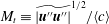$M_{t}\equiv \widetilde{|\boldsymbol{u}^{\prime \prime }\boldsymbol{u}^{\prime \prime }|}^{1/2}/\langle c\rangle$ ).

Inside the shock region, stresses reach a peak at a location where the pressure gradient is largest. Reynolds stresses then decrease and reach a downstream minimum where pressure attains a maximum. This location, identified as $2^{\prime }$ , indicates the end of the region dominated by shock compression. An expansion wave would follow behind the shock (Larsson & Lele Reference Larsson and Lele2009) where the stress reaches its downstream maximum. This process is dominated by pressure-dilatation exchanges that transfer internal energy to turbulent kinetic energy (Lee et al. Reference Lee, Lele and Moin1993). The Reynolds stresses increase but eventually viscous dissipation dominates the energy exchanges and turbulence undergoes again a classical viscous decay. The local maximum of $R_{11}$ downstream of the shock is denoted here by a subscript 2.

2.4 Resolution and DNS database

Table 1.

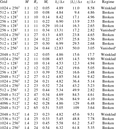
DNS database of isotropic turbulence (IT) passing through a shock: number of grid points, mean Mach number ( $M$ ), turbulent Mach ( $M_{t}$ ), Taylor Reynolds numbers ( $R_{\unicode[STIX]{x1D706}}$ ), normalized shock thicknesses and Kolmogorov length scale. The wrinkled and broken regimes correspond to the criterion in Donzis (Reference Donzis2012b ). Conditions for vanished regimes (marked with $^{\ast }$ ) are computed at the upstream minimum for pressure (§ 3.3).

Table 2.

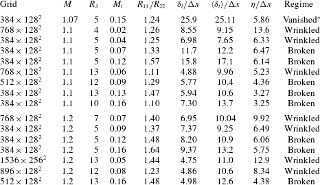
DNS database of anisotropic turbulence (SDT).

In table 1 we summarize the parameters for the simulations of STI with IT. The incoming turbulence is at turbulent Mach numbers ranging from 0.05 to 0.54 and Reynolds numbers up to 65. These parameters are obtained at location $x_{1}$ . The table also includes the ratio of Kolmogorov length scale to grid size $\unicode[STIX]{x1D702}/\unicode[STIX]{x0394}x$ , and the shock thickness to grid size, $\unicode[STIX]{x1D6FF}_{l}/\unicode[STIX]{x0394}x$ , where (Thompson Reference Thompson1984) $\unicode[STIX]{x1D6FF}_{l}=2k_{1}\langle \unicode[STIX]{x1D707}_{1}\rangle /(\langle c_{1}\rangle \langle \unicode[STIX]{x1D70C}_{1}\rangle \unicode[STIX]{x0394}M)$ with $k_{1}=(4/3+(\unicode[STIX]{x1D6FE}-1)/Pr)$ . In our simulations $k_{1}\sim O(1)$ . We have also included the classification of the regime of the interaction based on the mechanism in Donzis (Reference Donzis2012b ) where a transition from wrinkled to broken was proposed at $M_{t}/\unicode[STIX]{x0394}M\approx 0.6$ , consistent with the regimes observed in the literature (Larsson et al. Reference Larsson, Bermejo-Moreno and Lele2013; Ryu & Livescu Reference Ryu and Livescu2014).

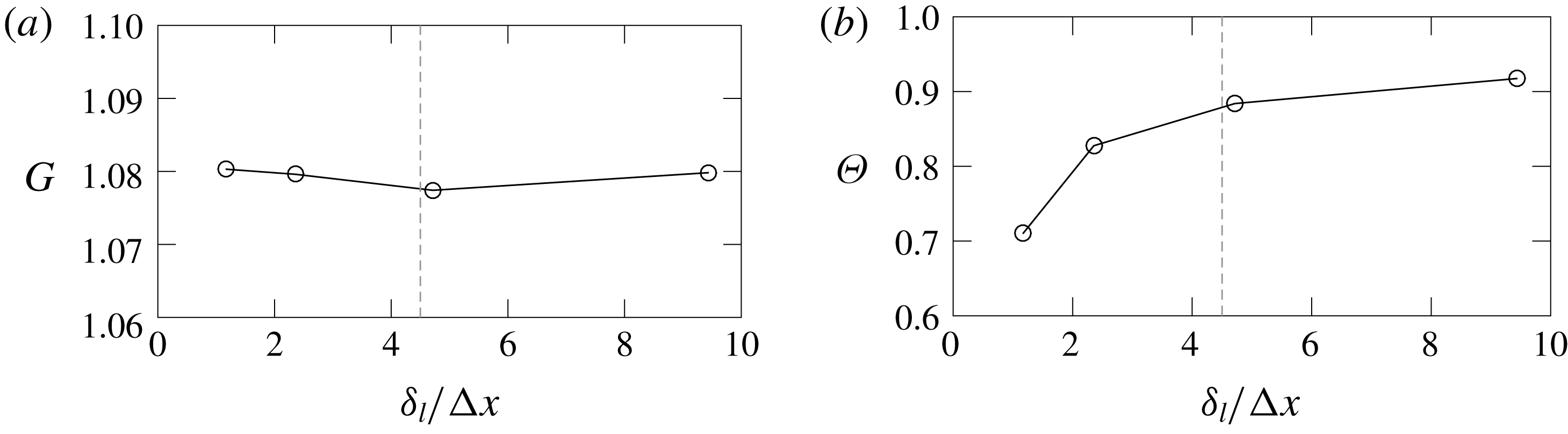
To ensure grid independence, convergence tests were conducted to assess the sensitivity of variables that characterize both large and, more critically, small scales. Two quantities that satisfy these requirements are the streamwise Reynolds stress, specifically its amplification factor, and the maximum dilatation at the shock. The latter is critically sensitive to resolution as it is computed at a location where gradients are largest (inside the viscous shock). In fact, this is a very strict resolution criterion but necessary for well-resolved shock-resolving simulations. In figure 3, we show the typical behaviour of the amplification factor of streamwise velocity, $G=R_{11,2}/R_{11,1}$ and r.m.s.-to-mean dilatation $\unicode[STIX]{x1D6E9}$ (Donzis Reference Donzis2012b ) as the ratio of shock thickness to grid spacing is increased. We see that beyond $\unicode[STIX]{x1D6FF}_{l}/\unicode[STIX]{x0394}x\approx 4.5$ , changes in these quantities are within 2 % and are thus considered grid converged. Similar results have been observed for the other conditions in our database. In addition, we have found (Jagannathan & Donzis Reference Jagannathan and Donzis2016) that a resolution of $\unicode[STIX]{x1D702}/\unicode[STIX]{x0394}x\approx 0.5$ is sufficient in isotropic turbulence to capture even fourth-order moments of velocity gradients at the conditions presented here. From tables 1 and 2 we can see that resolving the shock wave provides a stricter resolution criterion. In the table we also include $\langle \unicode[STIX]{x1D6FF}_{t}\rangle$ , the average thickness of the shock when turbulence is present (Donzis Reference Donzis2012b ) which is here computed as $(\langle u_{2}\rangle -\langle u_{1}\rangle )/(\unicode[STIX]{x2202}\langle u\rangle /\unicode[STIX]{x2202}x)_{max}$ . As expected and consistent with theoretical predictions (Donzis Reference Donzis2012b ), the difference between $\unicode[STIX]{x1D6FF}_{l}$ and $\langle \unicode[STIX]{x1D6FF}_{t}\rangle$ increases with $M_{t}$ . We do note that these definitions are estimates based on the maximum gradient at the shock and upon inspection represent only a fraction of the actual spatial extent occupied by the shock. In fact, even for the most stringent condition, at least 20 grid points are located between $x_{1}$ and $x_{2}$ (see figure 2). As mentioned above, however, this is for the most stringent cases and, as seen in the tables, most simulations have a larger number of grid points in the shock region. We have also verified grid convergence in the transverse direction since downstream of the shock, the Kolmogorov scale is reduced (Larsson & Lele Reference Larsson and Lele2009). At the most stringent conditions, we see a reduction of ${\sim}30\,\%$ in $\unicode[STIX]{x1D702}$ which when evaluated with our resolutions (tables 1 and 2) results in $\unicode[STIX]{x1D702}/\unicode[STIX]{x0394}y\approx 1.8$ which is also grid converged (Jagannathan & Donzis Reference Jagannathan and Donzis2016) for all cases here.

Figure 3.

Grid-independence test with different $\unicode[STIX]{x1D6FF}_{l}/\unicode[STIX]{x0394}x$ at $M=1.1$ , $M_{t}=0.21$ and $R_{\unicode[STIX]{x1D706}}\approx 25$ for (a) amplification factor and (b) r.m.s.-to-mean dilatation. The dashed line represents $\unicode[STIX]{x1D6FF}_{l}/\unicode[STIX]{x0394}x=4.5$ .

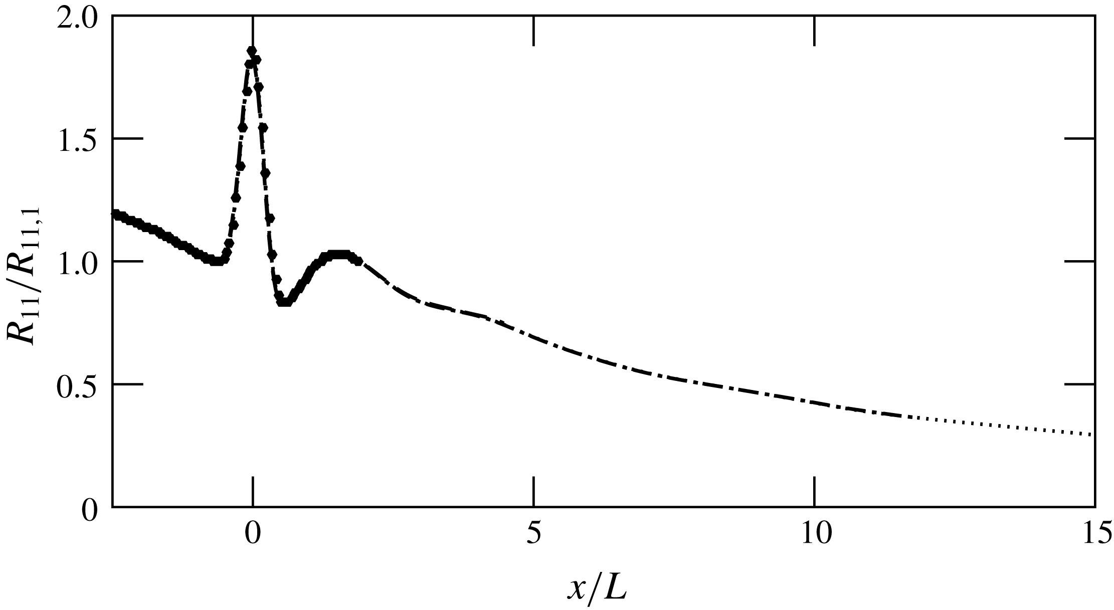
To ensure the sponges downstream of the shock have negligible effect on the interaction, we have conducted simulations with varying distance between the shock and the sponges, $\unicode[STIX]{x1D6E5}$ (see figure 1). The results are seen in figure 4 where we show the distribution of $R_{11}$ different values of $\unicode[STIX]{x1D6E5}$ . While all cases appear to collapse, some shock drifting is actually observed at $\unicode[STIX]{x1D6E5}=0.5\unicode[STIX]{x03C0}$ . 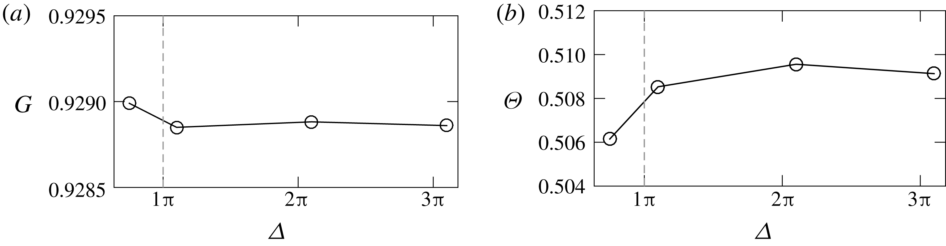This is more evident in figure 5 where we present $G$ and $\unicode[STIX]{x1D6E9}$ for different values of $\unicode[STIX]{x1D6E5}$ . Differences in this quantities for $\unicode[STIX]{x1D6E5}\gtrsim \unicode[STIX]{x03C0}$ are negligibly small. While data with $\unicode[STIX]{x1D6E5}=0.5\unicode[STIX]{x03C0}$ are also close, as a conservative measure especially at high $M_{t}$ , we have used $\unicode[STIX]{x1D6E5}=\unicode[STIX]{x03C0}$ . For reference, we mention that this distance corresponds to $\unicode[STIX]{x0394}\approx 2L$ where $L$ is the integral scale of the incoming turbulence.

Figure 4.

Distribution of $R_{11}$ at $M=1.2$ , $M_{t}=0.23$ and $R_{\unicode[STIX]{x1D706}}\approx 10$ with $\unicode[STIX]{x1D6E5}=0.5\unicode[STIX]{x03C0}$ (●), $1.1\unicode[STIX]{x03C0}$ (dashed), $2.2\unicode[STIX]{x03C0}$ (dash-dotted) and $3.3\unicode[STIX]{x03C0}$ (dotted).

Figure 5.

Test of distance between shock and sponges for (a) $G$ and (b) $\unicode[STIX]{x1D6E9}$ at $M=1.2$ , $M_{t}=0.23$ and $R_{\unicode[STIX]{x1D706}}\approx 10$ .

3.1 Theoretical background: quasi-equilibrium assumption and truncated integrals

Available results in the literature clearly show that characteristics of STI depend critically on the strength of turbulence (Andreopoulos et al. Reference Andreopoulos, Agui and Briassulis2000) which is not captured by LIA. The theoretical work of Moeckel (Reference Moeckel1952), Chisnell (Reference Chisnell1955), Whitham (Reference Whitham1958), is also unable to capture the complex behaviour of STI because of its simplified configuration and restrictive assumptions. An alternative view was more recently put forward (Donzis Reference Donzis2012b ), in which it was assumed that the shock, locally, adjusts instantaneously to local flow conditions. This was referred to as the quasi-equilibrium assumption. If conditions are such that QE is satisfied, a shock in a turbulent flow can be treated as consisting of a collection of infinitesimal shocks each obeying RH relations based on local flow conditions. For QE to be valid, the time scale associated with the relaxation of the shock to a new incoming condition should be much shorter than changes in upstream conditions produced by the turbulence. We showed (Donzis Reference Donzis2012b ) that this is justified when $K\ll 1$ which is satisfied for virtually all cases in the literature. The main advantage of QE is that it provides a framework in which well-known laminar results can be used to analytically compute mean variables in STI. In this section we use QE to provide analytical results for thermodynamic jumps across the shock. For strong turbulence, however, we first need to introduce a generalization of the analysis (Donzis Reference Donzis2012b ) which requires a redefinition of integrals to compute statistical moments across planes parallel to the shock surface.

Consider a shock in a uniform flow and a quantity $q$ that depends on the upstream Mach number, $M$ , that is $q=q(M)$ . In the presence of turbulent fluctuations, QE allows one to still write $q$ as a function of the local instantaneous Mach number, that is $q=q(M+m)$ where $m$ is the fluctuating Mach number. In general, the $n$ th-order moment of $q$ is given by the integral

(3.1) $$\begin{eqnarray}\langle q^{n}\rangle =\int _{-\infty }^{\infty }q^{n}(M+m)f_{m}(m)\,\text{d}m,\end{eqnarray}$$

where $f_{m}(m)$ is the probability density function (p.d.f.) of $m$ . Note that $M+m$ is to be taken as the relative velocity between the shock and the upstream flow. Thus, while here we consider a stationary shock, this formulation can account for moving shocks by a simple Galilean transformation.

However, the actual functional form of $q(M+m)$ may depend on whether the flow is supersonic or subsonic. For example, in locations where the flow is supersonic upstream of the mean location of the shock, the pressure will change according to the RH relations. However, if the flow is subsonic (due to strong negative $m$ fluctuations), then RH relations are invalid. This, as argued in Donzis (Reference Donzis2012b ), creates holes in the shock surface.

For the flow to be supersonic one needs $M+m>1$ or, in terms of $\unicode[STIX]{x0394}M=M-1$ , one needs $m>-\unicode[STIX]{x0394}M$ . Similarly subsonic regions correspond to fluctuations that satisfy $m<-\unicode[STIX]{x0394}M$ . Thus, we split the integral in (3.1) as

(3.2) $$\begin{eqnarray}\langle q^{n}\rangle =\int _{-\unicode[STIX]{x0394}M}^{\infty }(q^{{>}})^{n}f_{m}(m)\,\text{d}m+\int _{-\infty }^{-\unicode[STIX]{x0394}M}(q^{{<}})^{n}f_{m}(m)\,\text{d}m,\end{eqnarray}$$

where $q^{{>}}$ and $q^{{<}}$ are the functional form of $q$ in supersonic and subsonic regions, respectively. For short, the supersonic and subsonic integrals will be denoted by $\langle q^{n}\rangle ^{{>}}$ and $\langle q^{n}\rangle ^{{<}}$ , respectively, that is

(3.3) $$\begin{eqnarray}\langle q^{n}\rangle =\langle q^{n}\rangle ^{{>}}+\langle q^{n}\rangle ^{{<}}.\end{eqnarray}$$

One can, for example, compute moments of the fluctuating Mach number itself, i.e.  $q=m$ , for which supersonic and subsonic expressions are the same ( $q^{{>}}=q^{{<}}$ ). In this case we have:

(3.4a,b ) $$\begin{eqnarray}\langle m^{n}\rangle ^{{>}}=\int _{-\unicode[STIX]{x0394}M}^{\infty }m^{n}f_{m}(m)\,\text{d}m,\quad \langle m^{n}\rangle ^{{<}}=\int _{-\infty }^{-\unicode[STIX]{x0394}M}m^{n}f_{m}(m)\,\text{d}m.\end{eqnarray}$$

Obviously, $\langle m^{0}\rangle =1$ and $\langle m\rangle =0$ . Also note that by definition we can write the turbulent Mach number as:

(3.5) $$\begin{eqnarray}M_{t}=\sqrt{3}\langle m^{2}\rangle ^{1/2}=\sqrt{3}\left(\int _{-\infty }^{\infty }m^{2}f_{m}(m)\,\text{d}m\right)^{1/2}\end{eqnarray}$$

regardless of the specific velocity distribution.

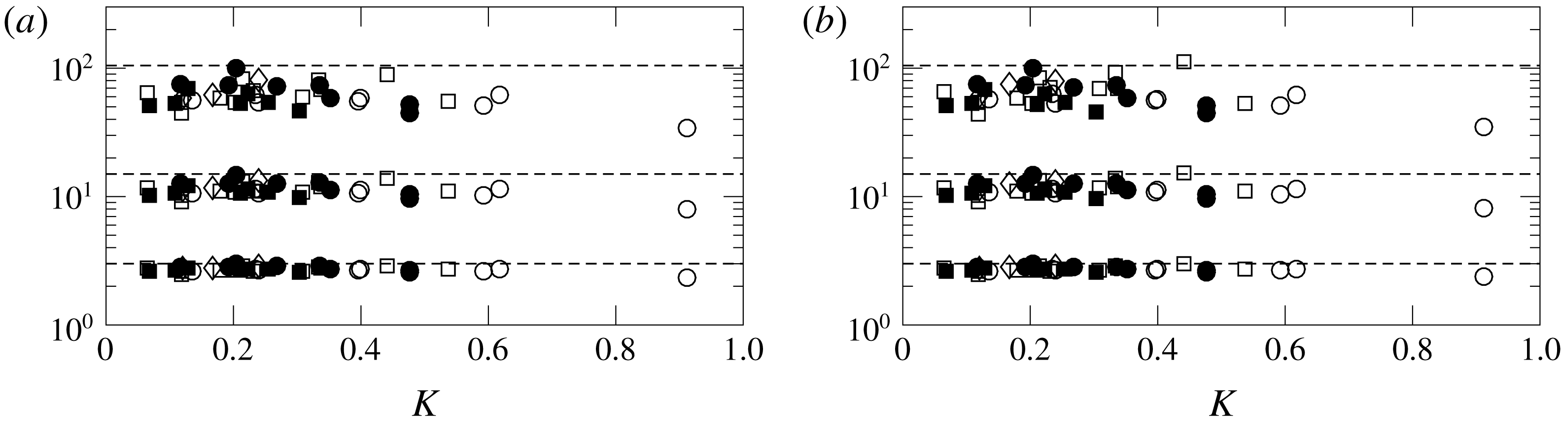
It is well known that the velocity field in isotropic turbulence is generally well represented by a Gaussian distribution (Batchelor Reference Batchelor1953; Monin & Yaglom Reference Monin and Yaglom1975). This is indeed the case for our data as seen in figure 6 where we show even moments of the streamwise velocity component and Mach number from our DNS database. Gaussian values are included as horizontal dashed lines for reference. We also see a slight sub-Gaussian behaviour for very high orders which has also been observed before (Noullez et al. Reference Noullez, Frisch, Wallace, Lempert and Miles1997; Jimenez Reference Jimenez1998). In any case, our results will rely on at most second-order statistics for which a Gaussian behaviour is an excellent approximation. For reference, the first few truncated moments of $m$ for a Gaussian distribution are shown in appendix A.

Figure 6.

Even moments of (a) velocity fluctuation $\langle u^{n}\rangle /\langle u^{2}\rangle ^{n/2}$ and (b) Mach number fluctuation $\langle m^{n}\rangle /\langle m^{2}\rangle ^{n/2}$ as functions of $K$ at location 1 for all the simulations in tables 1 and 2: $M=1.1$ (circles), $M=1.2$ (squares) and $M=1.4$ (diamonds). Open and closed symbols are for IT and SDT simulations. From bottom to top $n=4$ , 6 and 8. Dashed lines correspond to Gaussian values at 3, 15 and 105, respectively.

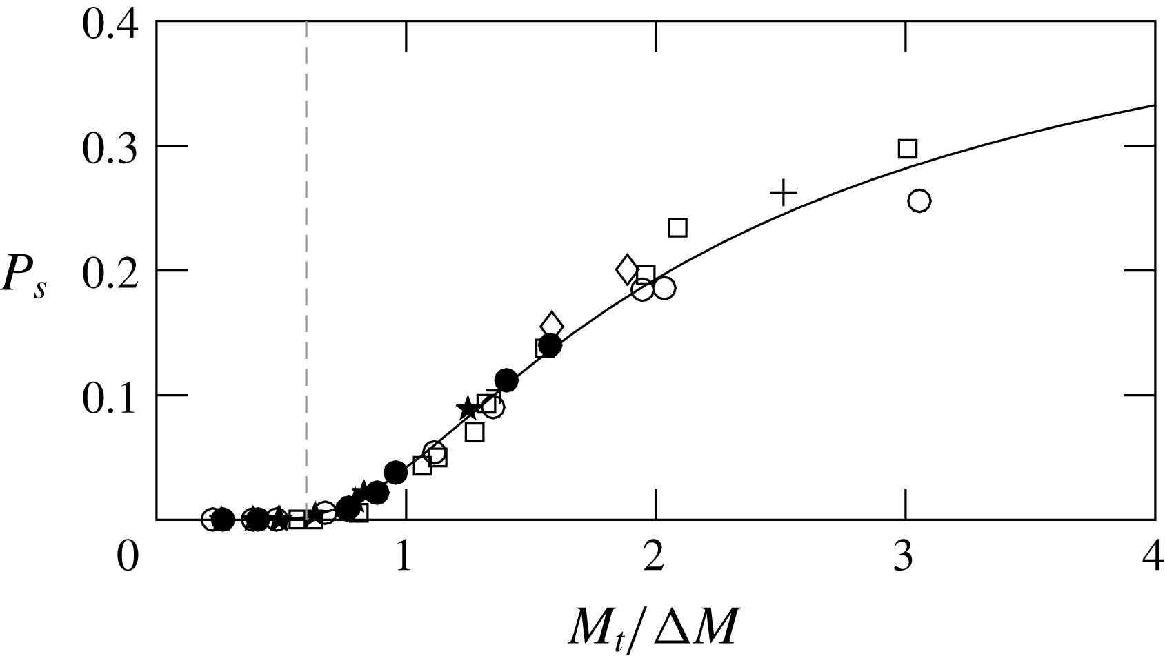
In Donzis (Reference Donzis2012b ) we argued that, consistent with QE, holes in the shocks are caused by locally subsonic conditions. Then $\langle m^{0}\rangle ^{{<}}$ would represent the fraction of the shock with subsonic regions and, thus, holes. This analytical form is shown in figure 7. One can see that the subsonic fraction upstream of the shock is negligible for $M_{t}/\unicode[STIX]{x0394}M\lesssim 0.6$ but grows quickly with $M_{t}/\unicode[STIX]{x0394}M$ beyond that. Thus, one expects to observe holes only at $M_{t}/\unicode[STIX]{x0394}M\gtrsim 0.6$ (Donzis Reference Donzis2012b ) in what is now called the broken regime. This criterion has indeed been supported by more recent DNS data (Larsson et al. Reference Larsson, Bermejo-Moreno and Lele2013). In the figure we also include results from our own DNS taken as the fraction of subsonic regions observed at $x_{1}$ . The excellent agreement supports both the Gaussian assumption for $m$ as well as the criterion $M_{t}/\unicode[STIX]{x0394}M=0.6$ to delineate the boundary between wrinkled and broken regimes. The last column in tables 1 and 2 indicates the regime based on this criterion.

Figure 7.

Probability of subsonic regions upstream of the shock. Solid line: theoretical $P_{s}=P(m<-\unicode[STIX]{x0394}M)$ with Gaussian p.d.f. for $m$ . Symbols for DNS data at $R_{\unicode[STIX]{x1D706}}\approx 5$ (stars), $R_{\unicode[STIX]{x1D706}}\approx 10$ (circles), $R_{\unicode[STIX]{x1D706}}\approx 25$ (squares), $R_{\unicode[STIX]{x1D706}}\approx 45$ (diamonds) and $R_{\unicode[STIX]{x1D706}}\approx 65$ (plus signs). Open and closed symbols are for IT and SDT simulations, respectively. Grey dashed line at $M_{t}/\unicode[STIX]{x0394}M=0.6$ for reference.

3.2 Analytical solutions of turbulent shock jumps

3.2.1 Density, pressure and temperature

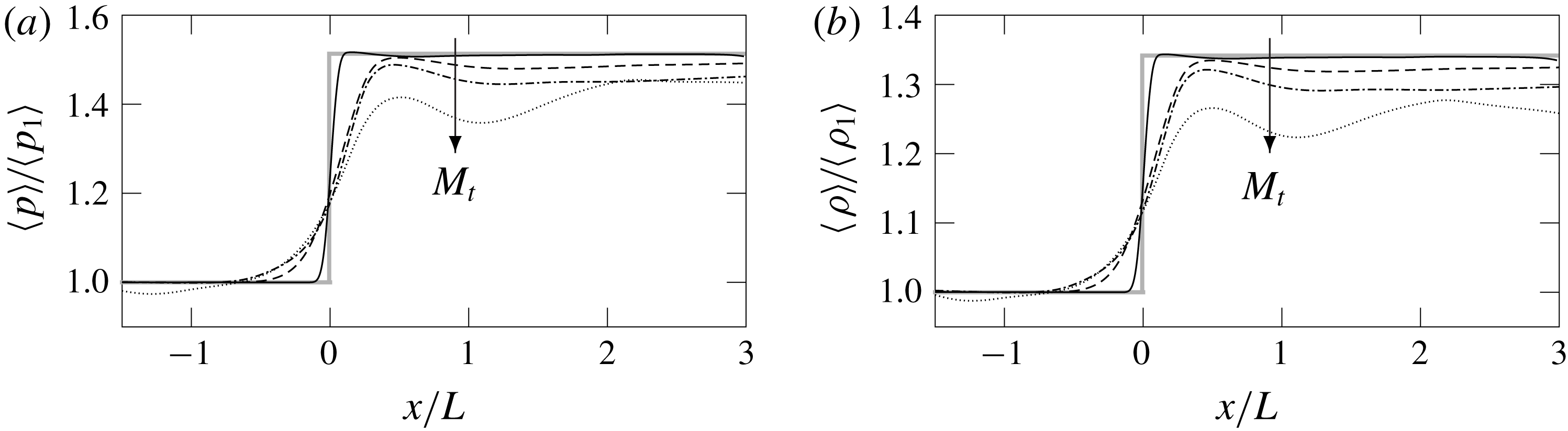
The Rankine–Hugoniot relations, which relate upstream and downstream conditions of a shock in a uniform flow, are a function of $M$ alone. In turbulent flows, however, fluctuations are found to modify these jumps, an effect that is more prominent as the strength of turbulence increases. This can be seen in figure 8 where we plot the distributions of pressure and density for different values of $M_{t}$ . As $M_{t}$ increases the jumps weaken compared to RH jumps (horizontal dotted lines) at a fixed $M$ . These results demonstrate that thermodynamic jumps depend not only on the mean flow but also on turbulent fluctuations. This effect is not captured by classical theories such as LIA whose results depend only on $M$ . Our objective here is to obtain analytical solutions for jumps of thermodynamic variables that can account for the effects of turbulence.

Figure 8.

(a) Pressure and (b) density profile of normal shocks interacting with isotropic turbulence at $M=1.2$ , $R_{\unicode[STIX]{x1D706}}\approx 25$ and $M_{t}=0.12$ (solid), 0.21 (dashed), 0.32 (dashed-dotted) and 0.44 (dotted). Grey lines correspond to the laminar inviscid limit, namely, RH jumps.

Consider first the ratio of mean density upstream and downstream of the shock, that is, $\langle \unicode[STIX]{x1D70C}_{2^{\prime }}\rangle /\langle \unicode[STIX]{x1D70C}_{1}\rangle$ . To compute this ratio we will obtain $\langle \unicode[STIX]{x1D70C}_{1}\rangle$ and $\langle \unicode[STIX]{x1D70C}_{2^{\prime }}\rangle$ in turn. We first note that in general the mean density ahead of a shock depends on the levels of fluctuations. A convenient way to account for this is to write the instantaneous density upstream of the shock in terms of stagnation conditions,

(3.6) $$\begin{eqnarray}\unicode[STIX]{x1D70C}_{1}=\left[\frac{\unicode[STIX]{x1D6FE}-1}{2}(M+m)^{2}+1\right]^{-1/(\unicode[STIX]{x1D6FE}-1)}\unicode[STIX]{x1D70C}_{01},\end{eqnarray}$$

where subscript 0 indicates a stagnation property. If fluctuations are isentropic, then $\unicode[STIX]{x1D70C}_{01}$ would be a constant across a plane parallel to the shock (over which averages are taken) independent of local Mach number fluctuations. This is in fact a very reasonable approximation for fluctuations not very far from the mean (Donzis & Jagannathan Reference Donzis and Jagannathan2013) and will, thus, be adopted here.

Expanding (3.6) in Taylor series around the mean Mach number yields:

(3.7) $$\begin{eqnarray}\unicode[STIX]{x1D70C}_{1}=\unicode[STIX]{x1D70C}_{1}|_{m=0}+\left(\frac{\unicode[STIX]{x2202}\unicode[STIX]{x1D70C}_{1}}{\unicode[STIX]{x2202}m}\right)_{m=0}m+\frac{1}{2}\left(\frac{\unicode[STIX]{x2202}^{2}\unicode[STIX]{x1D70C}_{1}}{\unicode[STIX]{x2202}m^{2}}\right)_{m=0}m^{2}+\cdots \,,\end{eqnarray}$$

whose average can then be computed by

(3.8) $$\begin{eqnarray}\langle \unicode[STIX]{x1D70C}_{1}\rangle =\int _{-\infty }^{\infty }\unicode[STIX]{x1D70C}_{1}\,f_{m}(m)\,\text{d}m.\end{eqnarray}$$

Combining (3.6)–(3.8) and a Gaussian $f_{m}(m)$ (see table 3) we can obtain the final form for the mean upstream density:

(3.9) $$\begin{eqnarray}\langle \unicode[STIX]{x1D70C}_{1}\rangle =\mathbb{M}^{-1/(\unicode[STIX]{x1D6FE}-1)}\unicode[STIX]{x1D70C}_{01}+{\textstyle \frac{1}{12}}\mathbb{M}^{(-2\unicode[STIX]{x1D6FE}+1)/(\unicode[STIX]{x1D6FE}-1)}[(\unicode[STIX]{x1D6FE}+1)M^{2}-2]\unicode[STIX]{x1D70C}_{01}M_{t}^{2},\end{eqnarray}$$

where, for simplicity in notation, we have defined $\mathbb{M}\equiv (\unicode[STIX]{x1D6FE}-1)M^{2}/2+1$ . The first term in (3.9) corresponds to the laminar contribution while the second term corresponds to turbulence effects which depend explicitly on both $M$ and $M_{t}$ . Clearly, as $M\rightarrow \infty$ or $M_{t}\rightarrow 0$ , the second term vanishes, as expected.

Under the QE assumption, the density immediately downstream of the shock (i.e. location $2^{\prime }$ ) will be given by RH expressions using the local Mach number, that is

(3.10) $$\begin{eqnarray}\unicode[STIX]{x1D70C}_{2^{\prime }}^{{>}}=\frac{(\unicode[STIX]{x1D6FE}+1)(M+m)^{2}}{(\unicode[STIX]{x1D6FE}-1)(M+m)^{2}+2}\unicode[STIX]{x1D70C}_{1}.\end{eqnarray}$$

The superscript $^{{>}}$ has been added to emphasize that shock relations are valid only for supersonic regions. Using (3.6), the expression becomes:

(3.11) $$\begin{eqnarray}\unicode[STIX]{x1D70C}_{2^{\prime }}^{{>}}=\left[\frac{(\unicode[STIX]{x1D6FE}+1)(M+m)^{2}}{(\unicode[STIX]{x1D6FE}-1)(M+m)^{2}+2}\right]\left[\frac{\unicode[STIX]{x1D6FE}-1}{2}(M+m)^{2}-1\right]^{-1/(\unicode[STIX]{x1D6FE}-1)}\unicode[STIX]{x1D70C}_{01}.\end{eqnarray}$$

In subsonic regions this expression is clearly invalid and, thus, averages need to be taken using the split form in (3.3). For subsonic regions, where shock holes appear, one can assume that variables will approximately retain their upstream value. That is, $\unicode[STIX]{x1D70C}_{2^{\prime }}^{{<}}\approx \unicode[STIX]{x1D70C}_{1}$ . This assumption is indeed supported by observations of instantaneous density profiles in the broken regime (e.g. Larsson & Lele Reference Larsson and Lele2009). Hence, the average downstream density is given by:

(3.12) $$\begin{eqnarray}\langle \unicode[STIX]{x1D70C}_{2^{\prime }}\rangle =\langle \unicode[STIX]{x1D70C}_{2^{\prime }}^{{>}}\rangle ^{{>}}+\langle \unicode[STIX]{x1D70C}_{1}\rangle ^{{<}}.\end{eqnarray}$$

Again, using Taylor series for (3.11) and substituting into (3.12) one can integrate the expressions analytically with $f_{m}(m)$ Gaussian, to obtain

(3.13) $$\begin{eqnarray}\displaystyle \langle \unicode[STIX]{x1D70C}_{2^{\prime }}\rangle & = & \displaystyle \left[\frac{(\unicode[STIX]{x1D6FE}+1)M^{2}}{(\unicode[STIX]{x1D6FE}-1)M^{2}+2}\right]\mathbb{M}^{-1/(\unicode[STIX]{x1D6FE}-1)}\unicode[STIX]{x1D70C}_{01}\langle m^{0}\rangle ^{{>}}-\frac{\unicode[STIX]{x1D6FE}+1}{2}M(M^{2}-2)\mathbb{M}^{(-2\unicode[STIX]{x1D6FE}+1)/(\unicode[STIX]{x1D6FE}-1)}\unicode[STIX]{x1D70C}_{01}\langle m\rangle ^{{>}}\nonumber\\ \displaystyle & & \displaystyle +\,\frac{\unicode[STIX]{x1D6FE}+1}{8}\mathbb{M}^{(-3\unicode[STIX]{x1D6FE}+2)/(\unicode[STIX]{x1D6FE}-1)}[(\unicode[STIX]{x1D6FE}+1)M^{4}-(6\unicode[STIX]{x1D6FE}+4)M^{2}+4]\unicode[STIX]{x1D70C}_{01}\langle m^{2}\rangle ^{{>}}\nonumber\\ \displaystyle & & \displaystyle +\,\mathbb{M}^{-1/(\unicode[STIX]{x1D6FE}-1)}\unicode[STIX]{x1D70C}_{01}\langle m^{0}\rangle ^{{<}}-M\mathbb{M}^{-\unicode[STIX]{x1D6FE}/(\unicode[STIX]{x1D6FE}-1)}\unicode[STIX]{x1D70C}_{01}\langle m\rangle ^{{<}}\nonumber\\ \displaystyle & & \displaystyle +\,\frac{1}{4}\mathbb{M}^{(-2\unicode[STIX]{x1D6FE}+1)/(\unicode[STIX]{x1D6FE}-1)}[(\unicode[STIX]{x1D6FE}+1)M^{2}-2]\unicode[STIX]{x1D70C}_{01}\langle m^{2}\rangle ^{{<}},\end{eqnarray}$$

which, though very complicated, provides an analytical closed form for the mean density downstream of a shock as a function of both $M$ and $M_{t}$ .

Thus the density jump across a shock in a turbulent flow with mean Mach number $M$ and turbulent Mach number $M_{t}$ can be written as

(3.14) $$\begin{eqnarray}\frac{\langle \unicode[STIX]{x1D70C}_{2^{\prime }}\rangle }{\langle \unicode[STIX]{x1D70C}_{1}\rangle }=g_{\unicode[STIX]{x1D70C}}(M,M_{t}),\end{eqnarray}$$

where $g_{\unicode[STIX]{x1D70C}}(M,M_{t})$ is the ratio of (3.13) and (3.6).

Figure 9.

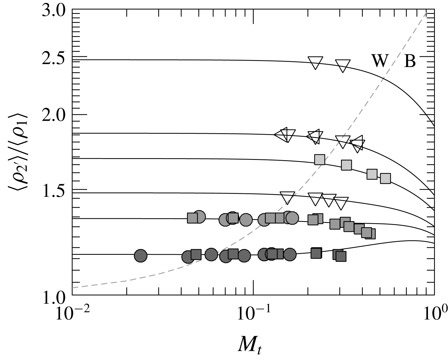
Mean density jumps from IT (squares) and SDT (circle) simulations at $M=1.1$ (dark), 1.2 (medium) and 1.4 (light). Other symbols are for Larsson & Lele (Reference Larsson and Lele2009) (▿), and Larsson et al. (Reference Larsson, Bermejo-Moreno and Lele2013) (◃). Solid lines correspond to the analytical solution (3.14) at $M=1.1$ , 1.2, 1.28, 1.4, 1.5 and 1.87 (bottom to top). Grey dashed line at $M_{t}/\unicode[STIX]{x0394}M=0.6$ separates the wrinkled (W) and broken (B) regimes.

In figure 9 we show $\langle \unicode[STIX]{x1D70C}_{2^{\prime }}\rangle /\langle \unicode[STIX]{x1D70C}_{1}\rangle$ from DNS data as a function of $M_{t}$ along with (3.14). We see very good agreement between DNS data from various sources (symbols) and the theoretical prediction (solid lines). As expected, laminar conditions are recovered as the turbulent Mach number decreases which is seen as solid lines approach their asymptotic RH value at $M_{t}\rightarrow 0$ . It is interesting to note that the effect of turbulent fluctuations depends on the mean Mach number as well. In particular, stronger turbulence effects are observed at higher $M$ . This suggests an interaction between means and fluctuations which is not accounted for in classical theories such as LIA. For relatively high $M$ , an increase in turbulence intensity measured by $M_{t}$ , results in weakened jumps relative to the laminar situation consistent with previous observations (Larsson et al. Reference Larsson, Bermejo-Moreno and Lele2013). It is worth mentioning here, that mean jumps are unaffected by turbulence within LIA and can thus not capture this behaviour. Predictions using RDT, in turn, were also found (Larsson et al. Reference Larsson, Bermejo-Moreno and Lele2013) to remain only qualitatively consistent with the data. The quantitative agreement between (3.14) and data observed in figure 9, thus, provides support to the adequacy of the QE coupled with the isentropic assumption of upstream fluctuations to capture this two-way coupling.

We also see a qualitative change in the effect of turbulence as $M$ decreases. For relatively weak shocks (low $M$ ) the theory predicts stronger shock jumps as turbulence intensity increases. Our DNS data do indeed show a consistent, though small, increase with $M_{t}$ . This low- $M$ conditions may be important in situations around transients crossing sonic conditions such as bodies, vanes or blades accelerating to supersonic speeds or decelerating to subsonic speeds. At $M\approx 1.2$ , jumps appear to be only weakly affected by turbulence with jumps remaining fairly constant with $M_{t}$ . This transition $M$ , however, is not general and depends on the value of $\unicode[STIX]{x1D6FE}$ .

In figure 9 we also show a (dashed) line at constant $M_{t}/\unicode[STIX]{x0394}M=0.6$ which separates the wrinkled (denoted W in the figure) and broken (denoted B) regimes (Donzis Reference Donzis2012b ). Conditions to the left of the WB line correspond to wrinkled interactions where the planar shock retains its structure and is only mildly distorted by the relatively weak incoming turbulent fluctuations. To the right of that line, the interaction is in the broken regime where holes appear across the shock. As $M_{t}$ is increased further, which implies also high $K$ , the fundamental assumptions behind QE will become progressively less applicable. These include the inability of the shock to adjust instantaneously to changing conditions due to turbulence fluctuations (Donzis Reference Donzis2012b ) as well as strong three-dimensional effects. This can explain the discrepancy seen between theory and DNS data for high- $M_{t}$ low- $M$ interactions in figure 9.

Following the same procedure described above, one can obtain expressions for $\langle p_{1}\rangle$ , $\langle p_{2^{\prime }}\rangle$ , $\langle T_{1}\rangle$ and $\langle T_{2^{\prime }}\rangle$ . The final result is

(3.15) $$\begin{eqnarray}\displaystyle & \displaystyle \frac{\langle p_{2^{\prime }}\rangle }{\langle p_{1}\rangle }=g_{p}(M,M_{t}), & \displaystyle\end{eqnarray}$$

(3.16) $$\begin{eqnarray}\displaystyle & \displaystyle \frac{\langle T_{2^{\prime }}\rangle }{\langle T_{1}\rangle }=g_{T}(M,M_{t}). & \displaystyle\end{eqnarray}$$

The details of the derivation and final expressions can be found in appendix A.

Figure 10.

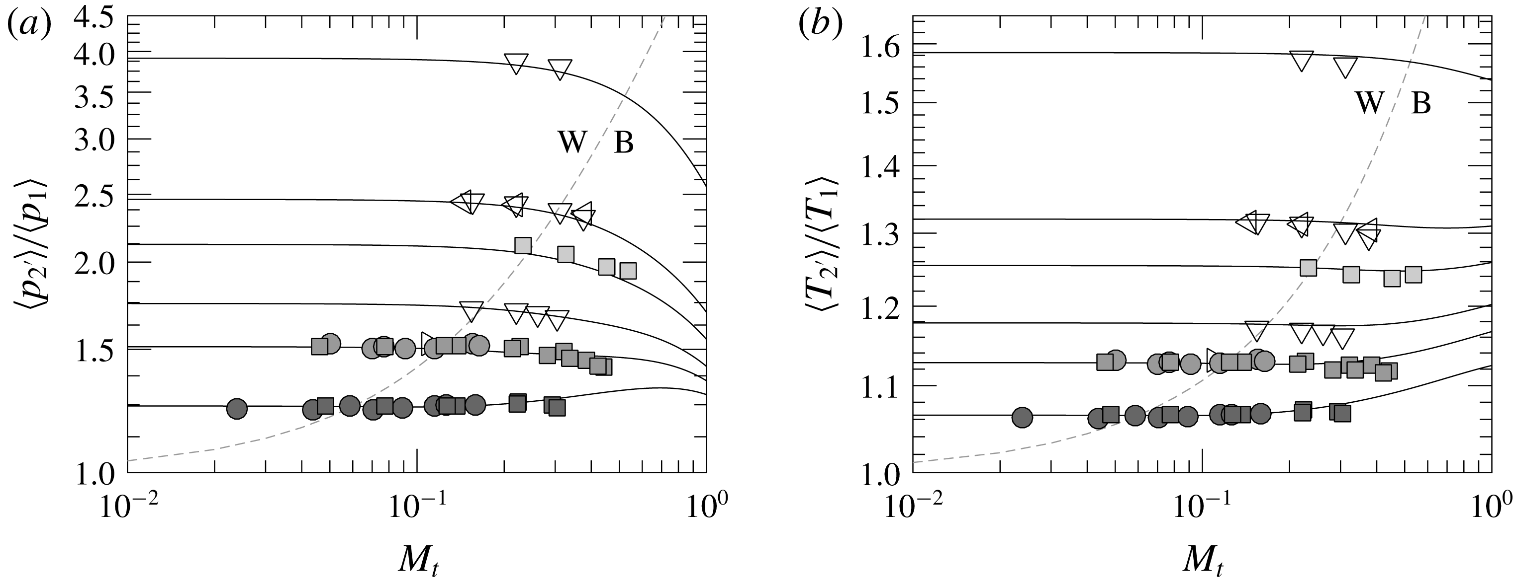
Mean pressure and temperature jumps from IT (squares) and SDT (circles) simulations, Lee et al. (Reference Lee, Lele and Moin1993) (▹), Larsson & Lele (Reference Larsson and Lele2009) (▿) and Larsson et al. (Reference Larsson, Bermejo-Moreno and Lele2013) (◃). Solid lines correspond to the analytical solution (A 5) at $M=1.1$ , 1.2, 1.28, 1.4, 1.5 and 1.87 (bottom to top). Grey dashed line at $M_{t}/\unicode[STIX]{x0394}M=0.6$ separates the wrinkled (W) and broken (B) regimes.

The comparison between DNS data and (3.15) and (3.16) is shown in figure 10. Again, good agreement is observed at a range of $M_{t}$ . While the behaviour of pressure is very similar to that of density we see that that of temperature is not. In fact, trends appear inverted: at low $M$ effects are stronger and jumps become larger as $M_{t}$ increases. At high $M$ , effects are weaker and there is a slight decrease in jumps as $M_{t}$ increases.

3.2.2 Comparison to Rankine–Hugoniot relations

While it has been argued in the literature that stronger turbulence leads to weakened shock jumps (Larsson & Lele Reference Larsson and Lele2009), the data presented here suggest a more complex interaction. In particular, whether turbulence weakens or strengthens shock jumps depends on the specific combination of $M_{t}$ and $M$ . The theoretical results here can, in fact, provide the necessary guidance to understand this observation. Consider the relative change of the density jump $\langle \unicode[STIX]{x1D70C}_{2^{\prime }}\rangle /\langle \unicode[STIX]{x1D70C}_{1}\rangle =g_{\unicode[STIX]{x1D70C}}(M,M_{t})$ with respect to the RH jump, $g_{\unicode[STIX]{x1D70C}}^{RH}(M)$ :

(3.17) $$\begin{eqnarray}R_{\unicode[STIX]{x1D70C}}(M,M_{t})=\frac{g_{\unicode[STIX]{x1D70C}}(M,M_{t})-g_{\unicode[STIX]{x1D70C}}^{RH}(M)}{g_{\unicode[STIX]{x1D70C}}^{RH}(M)}.\end{eqnarray}$$

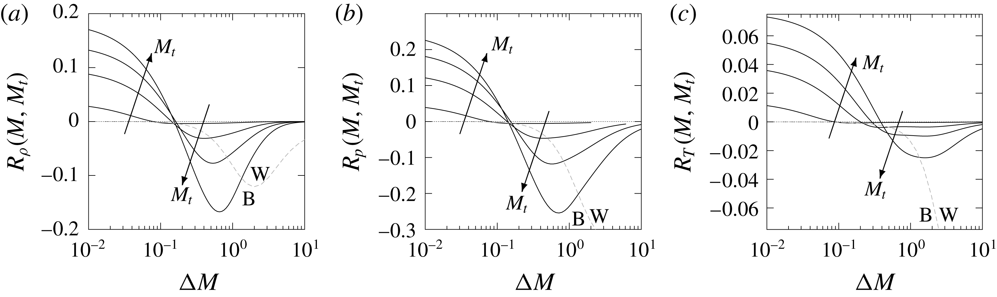
This function, which with (3.14) is known analytically, provides direct information of the effect of turbulence on the jumps of mean thermodynamic quantities. This is shown in figure 11(a) where we can now clearly see that turbulence effects on jumps depend on both $M$ and $M_{t}$ . In general for low $M$ , an increase of turbulence intensity ( $M_{t}$ ) leads to stronger shocks ( $R_{\unicode[STIX]{x1D70C}}(M,M_{t})>0$ ) relative to RH, or equivalently a shock in a uniform laminar flow at the same $M$ . However, as $M$ increases $R_{\unicode[STIX]{x1D70C}}(M,M_{t})$ changes sign and jumps become weaker. At higher $M$ , $R_{\unicode[STIX]{x1D70C}}(M,M_{t})$ decrease monotonically towards zero from below indicating a vanishing turbulence effect as $M\rightarrow \infty$ . A similar general behaviour is observed for the similarly defined $R_{p}(M,M_{t})$ and $R_{T}(M,M_{t})$ shown in figure 11.

Figure 11.

Relative departures from RH jumps for (a) density $R_{\unicode[STIX]{x1D70C}}(M,M_{t})$ , (b) pressure $R_{p}(M,M_{t})$ and (c) temperature $R_{T}(M,M_{t})$ at $M_{t}=0.1$ , 0.3, 0.5 and 0.8. Grey dashed line at $M_{t}/\unicode[STIX]{x0394}M=0.6$ separates the wrinkled (W) and broken (B) regimes.

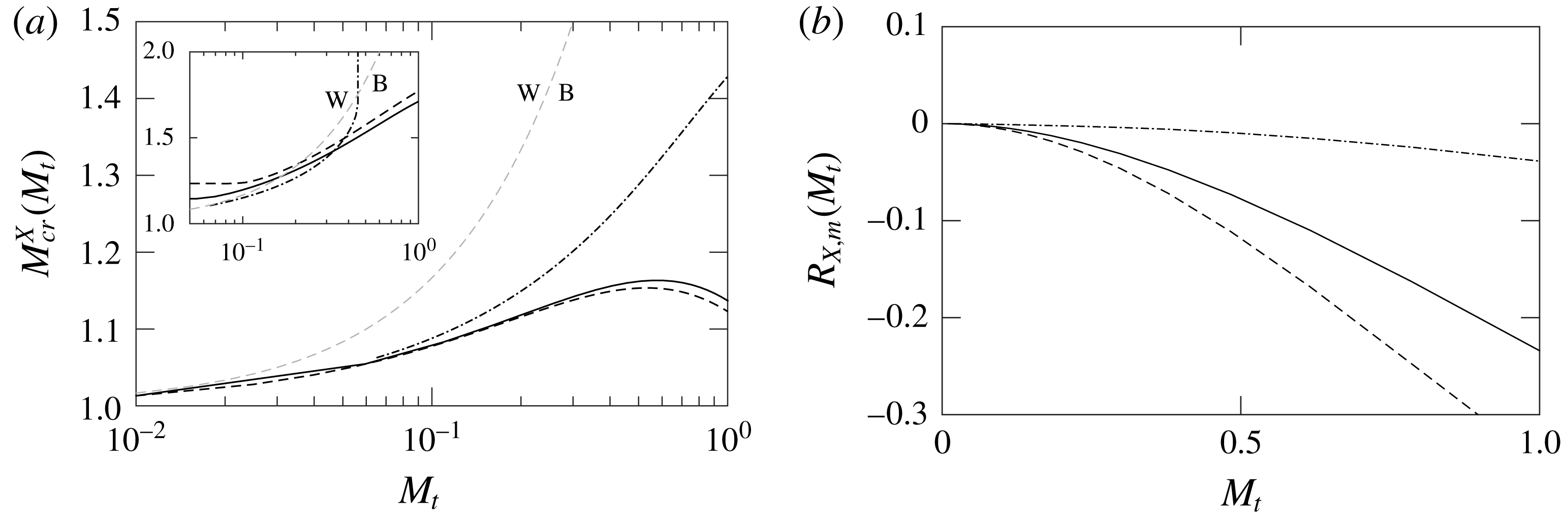
Two characteristic Mach numbers can now be identified for $R_{\unicode[STIX]{x1D70C}}(M,M_{t})$ . First, $M_{cr}^{\unicode[STIX]{x1D70C}}(M_{t})$ is the critical Mach number at which $R_{\unicode[STIX]{x1D70C}}(M,M_{t})$ changes sign. This can be readily found by solving $R_{\unicode[STIX]{x1D70C}}(M,M_{t})=0$ numerically for fixed $M_{t}$ . The result is shown in figure 12(a) along with the critical Mach numbers for pressure and temperature. We see that, while qualitatively similar, the critical Mach number is numerically different for $\unicode[STIX]{x1D70C}$ , $p$ and $T$ . Conditions below and above the corresponding $M_{cr}(M_{t})$ lines represent stronger and weaker shock jumps respectively for the different thermodynamic variables. We can also see that the critical Mach number appears mainly in the broken regime.

Figure 12.

(a) Critical Mach numbers ( $M_{cr}^{X}(M_{t})$ ) for density ( $X=\unicode[STIX]{x1D70C}$ , solid), pressure ( $X=p$ , dashed) and temperature ( $X=T$ , dash-dotted). Grey dashed line at $M_{t}/\unicode[STIX]{x0394}M=0.6$ separates the wrinkled (W) and broken (B) regimes. (b) Maximum weakening of shock jumps due to turbulence measured as the maximum relative departure from RH relations for density ( $X=\unicode[STIX]{x1D70C}$ , solid), pressure ( $X=p$ , dashed) and temperature ( $X=T$ , dash-dotted) for a given $M_{t}$ .

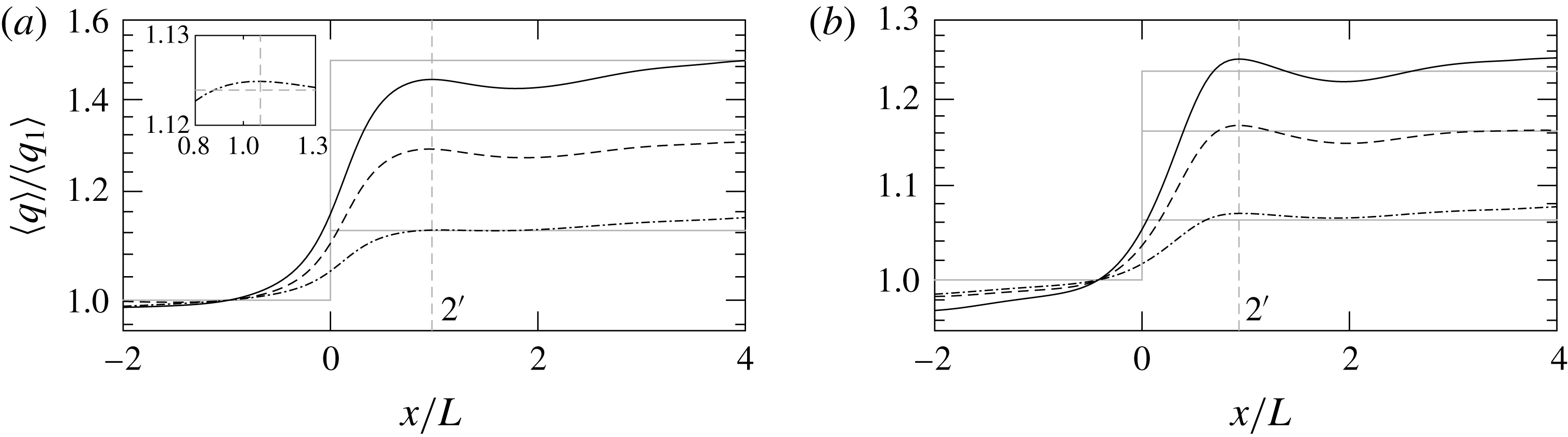
An interesting prediction by the theory is the existence of conditions at which pressure and density jumps are weakened by turbulence ( $M>M_{cr}^{\unicode[STIX]{x1D70C}}$ and $M>M_{cr}^{p}$ ) while temperature jumps are strengthened ( $M<M_{cr}^{T}$ ). This is indeed supported by our DNS data at $M_{t}=0.39$ and $M=1.2$ where temperature experiences an increase stronger than RH while pressure and density experience a weaker-than-RH increase across the shock. This is seen in figure 13(a) where we plot DNS data for this case along with corresponding RH jumps. In figure 13(b) we show a condition where all thermodynamic variables experience a stronger-than-RH jump due to turbulence.

Figure 13.

Variation of normalized pressure (solid, $q=p$ ), density (dashed, $q=\unicode[STIX]{x1D70C}$ ) and temperature (dash-dotted, $q=T$ ) across the shock. (a) $(M,M_{t},R_{\unicode[STIX]{x1D706}})\approx (1.2,0.39,13)$ which corresponds to $M<M_{cr}^{T}$ and $M>M_{cr}^{p},M_{cr}^{\unicode[STIX]{x1D70C}}$ Inset: detailed view of temperature around $x_{2^{\prime }}$ . (b) $(M,M_{t},R_{\unicode[STIX]{x1D706}})\approx (1.1,0.29,10)$ which corresponds to $M<M_{cr}^{T},M_{cr}^{p},M_{cr}^{\unicode[STIX]{x1D70C}}$ . Grey solid lines represent the laminar inviscid limits. Vertical grey dashed lines indicate the location of  $x_{2^{\prime }}$ .

A second characteristic Mach number is the location of the minimum observed for given $M_{t}$ in figure 11. This corresponds to the condition at which the largest turbulent effects are observed, and are denoted by $M_{m}^{\unicode[STIX]{x1D70C}}(M_{t})$ , $M_{m}^{p}(M_{t})$ and $M_{m}^{T}(M_{t})$ for density, pressure and temperature, respectively. These can be obtained by solving $\unicode[STIX]{x2202}R_{\unicode[STIX]{x1D70C}}(M,M_{t})/\unicode[STIX]{x2202}M=0$ and similar equations for density and pressure. The result is shown in the inset of figure 12(a). $M_{m}(M_{t})$ also is mainly in the broken regime though the three thermodynamic quantities lie close to each other and to the WB line. However, for higher $M_{t}$ we see $M_{m}^{T}(M_{t})$ grows substantially indicating that the strongest turbulence effect on temperature moves to higher values of  $M$ .

The analysis here also suggests that, for a fixed $M_{t}$ , there is a bound on how much a shock can be weakened by turbulence. This is given by the minimum value of $R_{\unicode[STIX]{x1D70C}}(M,M_{t})$ ( $R_{\unicode[STIX]{x1D70C},m}$ for short), which occurs at the second characteristic Mach number, that is $R_{\unicode[STIX]{x1D70C},m}\equiv R_{\unicode[STIX]{x1D70C}}(M_{m}^{\unicode[STIX]{x1D70C}}(M_{t}),M_{t})$ . This quantity is shown in figure 12(b) where we see that pressure jumps can be of the order of 30 % weaker at high $M_{t}$ . Weakening of temperature jumps however, are much smaller, staying below ${\sim}5$  % for the Mach numbers studied here. The Mach number at which this maximum effect is realized can be obtained from figure 11 or the full analytical expressions.

3.2.3 Entropy

Finally we turn to entropy which is also expected to contain both laminar and turbulent contributions. As before, one use QE to obtain the mean entropy jump across a shock as:

(3.18) $$\begin{eqnarray}\langle \unicode[STIX]{x0394}s\rangle =\langle \unicode[STIX]{x0394}s^{{<}}\rangle ^{{<}}+\langle \unicode[STIX]{x0394}s^{{>}}\rangle ^{{>}}.\end{eqnarray}$$

For supersonic regions, the standard entropy jump is $C_{p}\ln (T_{2^{\prime }}/T_{1})-R\ln (p_{2^{\prime }}/p_{1})$ which can also be written as

(3.19) $$\begin{eqnarray}\unicode[STIX]{x0394}s^{{>}}=C_{p}(\ln T_{2^{\prime }}-\ln T_{1})-R(\ln p_{2^{\prime }}-\ln p_{1}).\end{eqnarray}$$

The different terms can be computed as before. For example, the logarithm of the instantaneous temperature in terms of $M$ and $m$ is

(3.20) $$\begin{eqnarray}\ln T_{1}=\ln \left(\left[\frac{\unicode[STIX]{x1D6FE}-1}{2}(M+m)^{2}+1\right]^{-1}T_{01}\right),\end{eqnarray}$$

which upon expanding in Taylor series and averaging leads to:

(3.21) $$\begin{eqnarray}\displaystyle \langle \ln T_{1}\rangle ^{{>}} & = & \displaystyle \ln (\mathbb{M}^{-1})\langle m^{0}\rangle ^{{>}}-\frac{2(\unicode[STIX]{x1D6FE}-1)M}{(\unicode[STIX]{x1D6FE}-1)M^{2}+2}\langle m\rangle ^{{>}}\nonumber\\ \displaystyle & & \displaystyle +\,\frac{(\unicode[STIX]{x1D6FE}-1)[(\unicode[STIX]{x1D6FE}-1)M^{2}-2]}{[(\unicode[STIX]{x1D6FE}-1)M^{2}+2]^{2}}\langle m^{2}\rangle ^{{>}}+\ln T_{01}\langle m^{0}\rangle ^{{>}}.\end{eqnarray}$$

We can similarly obtain $\langle \ln T_{2^{\prime }}\rangle ^{{>}}$ , $\langle \ln p_{1}\rangle ^{{>}}$ and $\langle \ln p_{2^{\prime }}\rangle ^{{>}}$ .

For subsonic regions where there is no shock, the entropy increase will be solely due to the dissipative nature of turbulence. Obukhov (Reference Obukhov1949) showed that entropy generation due to turbulent fluctuations in temperature is proportional to the temperature variance. Specifically he showed that when the flow decays from a state characterized by a temperature variance $\langle T^{\prime 2}\rangle$ , the total entropy increase is $\langle \unicode[STIX]{x0394}s\rangle \approx C_{p}\langle {T^{\prime }}^{2}\rangle /\langle T\rangle ^{2}$ . In the present case, turbulence will not be completely dissipated as it crosses the shock region and reaches $x_{2^{\prime }}$ . However, it is still expected that the entropy increase will be proportional to the variance of temperature of the incoming flow. Furthermore, this variance can be written in terms of the turbulent Mach number as $\langle T^{\prime 2}\rangle /\langle T\rangle ^{2}\approx (A^{2}/9)(\unicode[STIX]{x1D6FE}-1)^{2}M_{t}^{4}$ (Donzis & Jagannathan Reference Donzis and Jagannathan2013). Thus, for holes one can expect

(3.22) $$\begin{eqnarray}\unicode[STIX]{x0394}s^{{<}}=\unicode[STIX]{x1D6FC}_{s}C_{p}(\unicode[STIX]{x1D6FE}-1)^{2}M_{t}^{4},\end{eqnarray}$$

where all prefactors are absorbed in the constant $\unicode[STIX]{x1D6FC}_{s}$ .

Finally, with (3.19) and (3.22) we take the conditional averages for the two regions as in (3.18) to obtain

(3.23) $$\begin{eqnarray}\frac{\langle \unicode[STIX]{x0394}s\rangle }{C_{p}}=g_{s}(M,M_{t}).\end{eqnarray}$$

The final expressions that comprise the function $g_{s}(M,M_{t})$ are explicitly shown in appendix A.

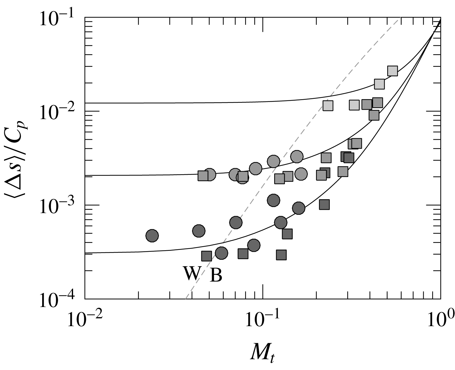
The DNS data of entropy jump across the shock along with the theoretical prediction (3.23) are shown in figure 14. The comparison shows good agreement though there is some scatter in the data. At very low $M_{t}$ , the change of entropy is due entirely to the well-known laminar jumps (Thompson Reference Thompson1984). As $M_{t}$ increases, we see a substantial increase in entropy production in both DNS data and the theoretical prediction (3.23).

Figure 14.

Mean entropy increase from IT (▪) and SDT (●) simulations. Solid lines correspond to the analytical solution (3.23) at $M=1.1$ , 1.2, and 1.4 (bottom to top) with $\unicode[STIX]{x1D6FC}_{s}=1.176$ . Grey dashed line at $M_{t}/\unicode[STIX]{x0394}M=0.6$ separates the wrinkled (W) and broken (B) regimes.

The theoretical result approaches an asymptotic $M_{t}^{4}$ at high $M_{t}$ indicating that turbulence entropy generation becomes the dominant contribution. Note that the supersonic regions also contains ‘turbulence effects’: this is seen, for example, from the second term in (3.21) which vanishes as the incoming flow fluctuations weakens ( $M_{t}\rightarrow 0$ ). However, the asymptotic behaviour of these terms is a weaker power law than $M_{t}^{4}$ . Furthermore, the entropy increase through shock holes is independent of the mean Mach number as it only reflects entropy production due to turbulent dissipation. Thus, the observed decreasing gap between curves at different $M$ as $M_{t}$ increases is also supportive of an increasingly dominant contribution from turbulent decay.

3.3 Shock structure

The effects of turbulence on shock characteristics have been studied theoretically in the literature (Ribner Reference Ribner1954a ,Reference Ribner b ; Williams & Howe Reference Williams and Howe1973; Zank et al. Reference Zank, Zhou, Matthaeus and Rice2002; Wouchuk, de Lira & Velikovich Reference Wouchuk, de Lira and Velikovich2009) and observed experimentally (Hesselink & Sturtevant Reference Hesselink and Sturtevant1988) and numerically (Lee et al. Reference Lee, Lele and Moin1993; Larsson & Lele Reference Larsson and Lele2009). These investigations helped identified two regimes – wrinkled and broken – which result from different levels of turbulence intensity. The former corresponds to an interaction in which the shock retains its structure as a sharp gradient over a weakly modified uniform shock plane. The latter corresponds to a strongly modified shock plane with ‘holes’ through which properties may change smoothly or have multiple peaks (Hesselink & Sturtevant Reference Hesselink and Sturtevant1988; Lee et al. Reference Lee, Lele and Moin1993).

A quantitative metric that has been used to characterize inhomogeneities in the structure of the shock is the r.m.s.-to-mean dilatation at the shock (Lee et al. Reference Lee, Lele and Moin1993; Larsson & Lele Reference Larsson and Lele2009)

(3.24) $$\begin{eqnarray}\unicode[STIX]{x1D6E9}=\left(\frac{\langle \unicode[STIX]{x1D703}_{s}^{2}\rangle _{s}}{\langle \unicode[STIX]{x1D703}_{s}\rangle _{s}^{2}}-1\right)^{1/2},\end{eqnarray}$$

where $\unicode[STIX]{x1D703}_{s}$ is the dilatation at the shock location which is identified as the largest negative value of dilation along the streamwise direction $x$ for a given location $(y,z)$ . That is, $\unicode[STIX]{x1D703}_{s}(y,z)=min_{x}\unicode[STIX]{x1D703}(x,y,z)$ . Note that since the location where $\unicode[STIX]{x1D703}$ attains its minimum is, in general, different for different locations $(y,z)$ , the averages in (3.24) are not over planes at fixed $x$ , but instead over all $\unicode[STIX]{x1D703}_{s}(y,z)$ – we use the additional subscript $s$ in $\langle \cdot \rangle _{s}$ , to differentiate it from plane averages $\langle \cdot \rangle$ . DNS data presented below are also time averaged.

Following Donzis (Reference Donzis2012b ), one can write the maximum negative dilatation at the shock as $\unicode[STIX]{x1D703}_{s}\approx \unicode[STIX]{x27E6}u\unicode[STIX]{x27E7}/\unicode[STIX]{x1D6FF}_{t}$ where $\unicode[STIX]{x27E6}u\unicode[STIX]{x27E7}$ is the velocity change across the shock and $\unicode[STIX]{x1D6FF}_{t}$ the shock thickness which, to leading order, can be written as $(\unicode[STIX]{x1D70C}c/\unicode[STIX]{x1D707})\unicode[STIX]{x27E6}u\unicode[STIX]{x27E7}(\unicode[STIX]{x0394}M+m)$ . Using unconditional averages over the entire surface and assuming $\unicode[STIX]{x27E6}u\unicode[STIX]{x27E7}$ is, to leading order, not affected by fluctuations, QE leads to $\langle \unicode[STIX]{x1D703}_{s}\rangle _{s}\sim (\langle \unicode[STIX]{x1D70C}_{1}\rangle \langle c_{1}\rangle /\langle \unicode[STIX]{x1D707}_{1}\rangle )\unicode[STIX]{x27E6}u\unicode[STIX]{x27E7}\unicode[STIX]{x0394}M$ and $\langle \unicode[STIX]{x1D703}_{s}^{2}\rangle _{s}\sim (\langle \unicode[STIX]{x1D70C}_{1}\rangle \langle c_{1}\rangle /\langle \unicode[STIX]{x1D707}_{1}\rangle )^{2}\unicode[STIX]{x27E6}u\unicode[STIX]{x27E7}^{2}(\unicode[STIX]{x0394}M^{2}+M_{t}^{2}/3)$ which, when used in (3.24), leads to:

(3.25) $$\begin{eqnarray}\unicode[STIX]{x1D6E9}\approx \frac{1}{\sqrt{3}}\frac{M_{t}}{\unicode[STIX]{x0394}M}.\end{eqnarray}$$

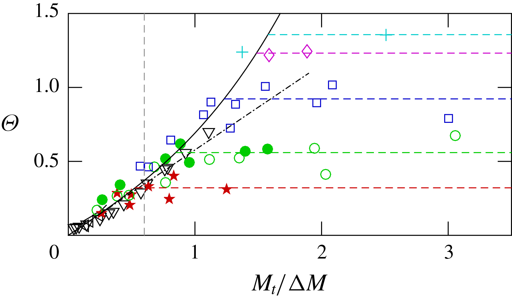
This has been shown to provide good collapse of the existing data (Donzis Reference Donzis2012b ; Boukharfane, Bouali & Mura Reference Boukharfane, Bouali and Mura2018). However, equation (3.25) is expected to be accurate only when turbulence is relatively weak. This is indeed the case as seen in figure 15, where we show $\unicode[STIX]{x1D6E9}$ for the present data (in colour) along with other existing data. The dash-dotted line is (3.25) while the solid line contains the next-order term in the expansion (Donzis Reference Donzis2012b ), that is $\unicode[STIX]{x1D6E9}\approx e_{1}M_{t}/\unicode[STIX]{x0394}M+e_{2}(M_{t}/\unicode[STIX]{x0394}M)^{3}$ where $e_{1}$ and $e_{2}$ are fitting constants. There is good agreement between the data and the theory in the wrinkled regime ( $M_{t}/\unicode[STIX]{x0394}M\lesssim 0.6$ ) consistent with previous studies (Donzis Reference Donzis2012b ; Boukharfane et al. Reference Boukharfane, Bouali and Mura2018).

As $M_{t}/\unicode[STIX]{x0394}M$ increases, however, departures are apparent with two interesting features. First we see that, in spite of significant scatter, $\unicode[STIX]{x1D6E9}$ seems to approach an asymptotic value ( $\unicode[STIX]{x1D6E9}_{\infty }$ ) at high $M_{t}/\unicode[STIX]{x0394}M$ with a value dependent on the Reynolds number. Second, DNS data depart from the QE prediction at higher $M_{t}/\unicode[STIX]{x0394}M$ when $R_{\unicode[STIX]{x1D706}}$ is high. This effect does not appear to be due to the increase of holes in the shock since figure 7 shows that the fraction of subsonic regions does not depend on $R_{\unicode[STIX]{x1D706}}$ . A potential explanation for this effect is that at low $R_{\unicode[STIX]{x1D706}}$ , stronger viscous effects enhance transverse diffusion of momentum which would make the one-dimensional local behaviour assumption in QE less applicable. However, a thorough verification of this explanation requires more data at a wide range of parameters.

Figure 15.

R.m.s.-to-mean dilatation at the shock for $R_{\unicode[STIX]{x1D706}}\approx 5$ (red stars), $R_{\unicode[STIX]{x1D706}}\approx 10$ (green circles), $R_{\unicode[STIX]{x1D706}}\approx 25$ (blue squares), $R_{\unicode[STIX]{x1D706}}\approx 45$ (magenta diamonds), $R_{\unicode[STIX]{x1D706}}\approx 65$ (cyan pluses). Open and closed symbols are for IT and SDT simulations, respectively. Vertical grey dashed line at $M_{t}/\unicode[STIX]{x0394}M=0.6$ for reference. Horizontal dashed lines: average of DNS data at high $M_{t}/\unicode[STIX]{x0394}M$ for $R_{\unicode[STIX]{x1D706}}\approx 5$ , 10, 25, 45 and 65 from bottom to top. Other symbols: Jamme et al. (Reference Jamme, Cazalbou, Torres and Chassaing2002) ( $\times$ ), Larsson & Lele (Reference Larsson and Lele2009) (▿) and Boukharfane et al. (Reference Boukharfane, Bouali and Mura2018) (◃).

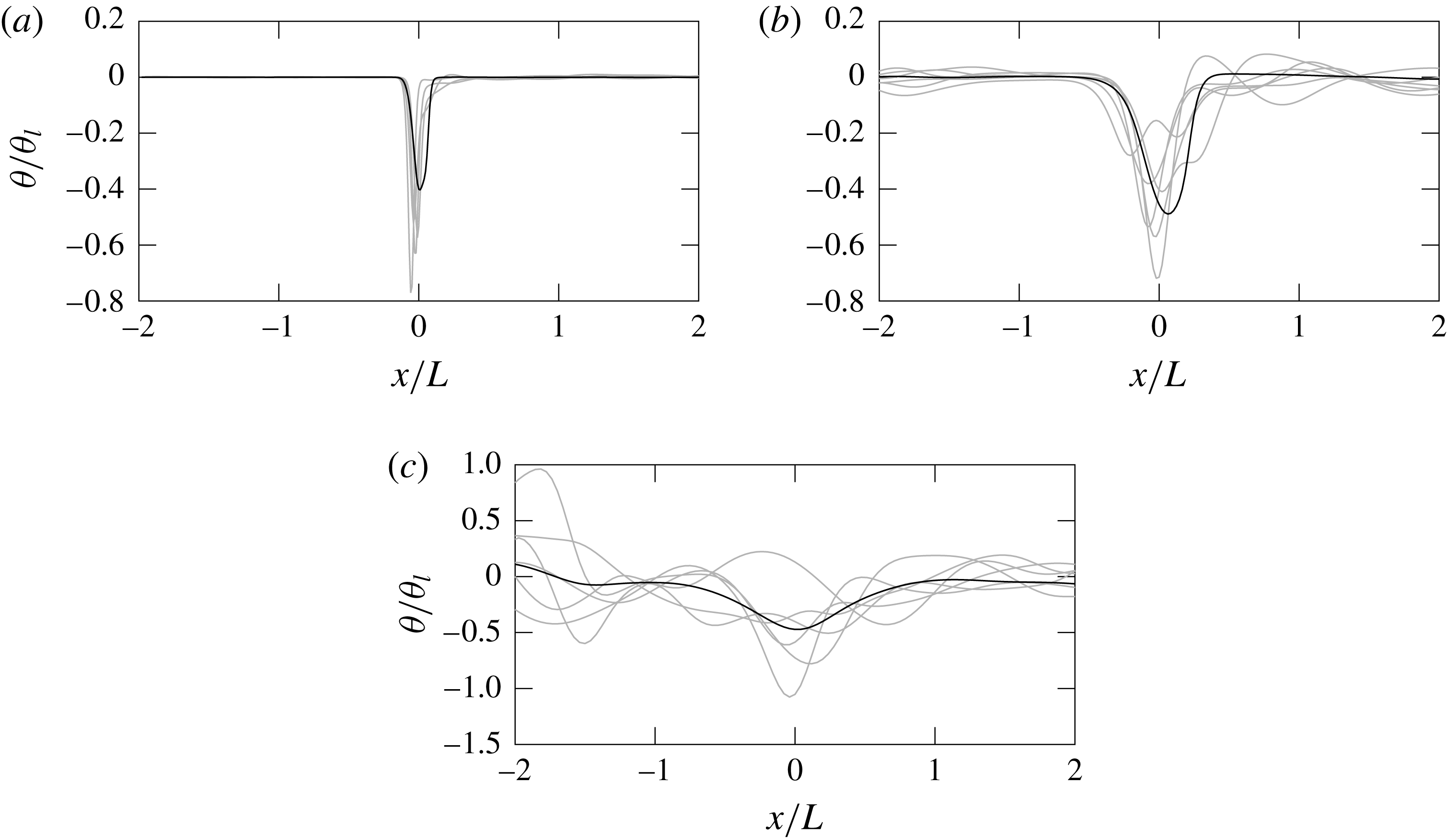
Before we discuss the asymptotic value $\unicode[STIX]{x1D6E9}_{\infty }$ , it is instructive to see the structure of the flow as it crosses the shock. In figure 16 we show, for three different cases, plane-averaged dilatation along the streamwise direction (dark line) with a set of instantaneous dilatation profiles at some arbitrary locations (light grey lines). In (a) we show a wrinkled case (though close to broken limit) with a very strong mean dilatation comprised of similar instantaneous profiles. At higher $M_{t}/\unicode[STIX]{x0394}M$ in the broken regime (b) we also see a strong peak though spatially broader, consistent with theoretical predictions (Donzis Reference Donzis2012b ). Individual dilatation profiles, however, display a wider range of behaviours: some have the same qualitative peak while others present multiple peaks or a very broad smooth variation (Lee et al. Reference Lee, Lele and Moin1993; Larsson & Lele Reference Larsson and Lele2009). At even higher values of $M_{t}/\unicode[STIX]{x0394}M$ (c) individual profiles show very large fluctuations upstream and downstream of the shock comparable to the mean (dark line). It is interesting to note that while fluctuations in this case are of the same order as the mean, the latter still shows the same peak as, although much broader than, in the wrinkled regime.

Figure 16.

Instantaneous dilatation normalized by laminar condition ( $\unicode[STIX]{x1D703}_{l}$ ) along the streamwise direction at different transverse locations (grey) and their mean (black) at $M=1.1$ , $R_{\unicode[STIX]{x1D706}}\approx 10$ and (a) $M_{t}=0.05$ (wrinkled), (b) $M_{t}=0.14$ (broken) and (c) $M_{t}=0.34$ (vanished).

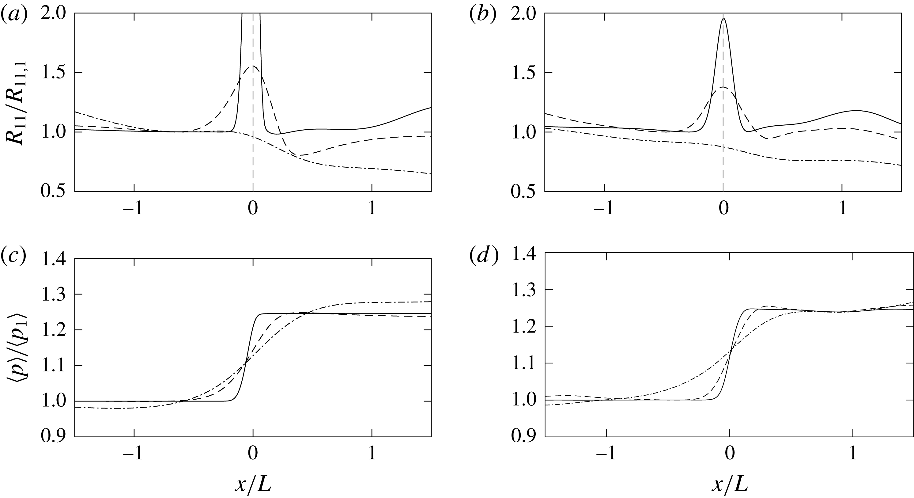
Typical distributions of Reynolds stresses and mean pressure are shown in figure 17 at similar conditions. In (a) and (b) we see that, consistent with observations in the literature, the downstream peak of $R_{11}$ at $x_{2}$ decreases with $M_{t}$ . As $M_{t}$ increases further, we observe both the peaks upstream and downstream of the shock ( $x_{1}$ and $x_{2}$ , respectively) vanish. We term this, then, the ‘vanished’ regime. Clearly in this regime, it is not possible to compute amplification factors since no upstream and downstream locations can be identified unambiguously as Reynolds stresses undergo a classical turbulent decay. It is interesting that other mean quantities such as mean pressure (c,d) or mean velocity retain the typical qualitative behaviour of a shock. While these mean gradients may lead to production by mean shear in the Reynolds stress budget, because of the short residence time within the shock region, they cannot, on average, counteract the viscous decay.

Furthermore, since in the vanished regime no $x_{1}$ location can be identified, it is also not possible to determine $R_{\unicode[STIX]{x1D706}}$ , $M_{t}$ or $\unicode[STIX]{x0394}M$ upstream of the shock. Alternatively, one can estimate them by assessing the limit at which local extrema vanish for $R_{11}$ . For example, for $R_{\unicode[STIX]{x1D706}}\approx 5$ , 10 and 25, we find that the vanished regime appears at $M_{t}/\unicode[STIX]{x0394}M\approx 2.14$ , 3.4 and 4.4, respectively. In these three cases, $K$ is found to be very close to 1.0. This is, in fact, not unexpected. As we show below, the amplification factor for $R_{11}$ shows a universal behaviour with $K$ for relatively high $K$ . In particular, it decreases with $K$ and reaches values around 0.8 at $K\approx 1$ . Beyond this value of $K$ no local extrema are observed and amplification factors cannot be obtained.

Figure 17.

Distributions of $R_{11}$ at $M=1.1$ , (a) $R_{\unicode[STIX]{x1D706}}\approx 10$ and $M_{t}=0.05$ (solid), $M_{t}=0.14$ (dashed) and $M_{t}=0.34$ (dash-dotted) and (b) $R_{\unicode[STIX]{x1D706}}\approx 25$ and $M_{t}=0.22$ (solid), $M_{t}=0.3$ (dashed) and $M_{t}=0.44$ (dash-dotted). Distribution of $p$ at (c) $R_{\unicode[STIX]{x1D706}}\approx 10$ and $M_{t}=0.05$ (solid), $M_{t}=0.14$ (dashed) and $M_{t}=0.34$ (dash-dotted) and (d) $R_{\unicode[STIX]{x1D706}}\approx 25$ and $M_{t}=0.22$ (solid), $M_{t}=0.3$ (dashed) and $M_{t}=0.44$ (dash-dotted).

We now get back to the asymptotic value $\unicode[STIX]{x1D6E9}_{\infty }$ . As $M_{t}/\unicode[STIX]{x0394}M$ increases, increasingly large areas of the shock are subsonic and present holes. However, it is unclear what the value of $\unicode[STIX]{x1D703}_{s}$ is across holes. Furthermore, as turbulence becomes more intense, the flow will experience stronger locally three-dimensional effects which will favour strong mixing in all directions and thus weaken the applicability of QE. According to the definition of $\unicode[STIX]{x1D6E9}$ one searches for the largest negative dilatation around the location of the shock along $x$ for a given $(y,z)$ location. When turbulence is strong (see instantaneous profiles in figure 16 c), one would expect $\unicode[STIX]{x1D6E9}$ to be essentially dominated by turbulence statistics and we can then use known scaling laws for velocity gradients. However, $\unicode[STIX]{x1D6E9}$ is based on the average of the minimum dilatation close to the average location of the shock. While the mean dilatation in isotropic turbulence is zero, the average of minimum dilatation across an arbitrary plane is not. Thus, we make the additional assumption that these values are, to first approximation, proportional to the average magnitude of those gradients. Moments of velocity gradients are known to scale as power laws with the Reynolds number (Monin & Yaglom Reference Monin and Yaglom1975): $\langle |\unicode[STIX]{x2202}u/\unicode[STIX]{x2202}x|^{n}\rangle =C_{n}(u_{1,rms}/L)^{n}R_{\unicode[STIX]{x1D706}}^{2d_{n}}$ where $C_{n}$ are flow-dependent constants and $d_{n}$ are the so-called scaling exponents. While these power laws have been historically believed to hold only for high Reynolds numbers, recent work suggests that their applicability extends to rather low Reynolds numbers (Schumacher, Sreenivasan & Yakhot Reference Schumacher, Sreenivasan and Yakhot2007; Schumacher et al. Reference Schumacher, Scheel, Krasnov, Donzis, Yakhot and Sreenivasan2014; Yakhot & Donzis Reference Yakhot and Donzis2017). We then estimate $\unicode[STIX]{x1D6E9}_{\infty }$ , when turbulence dominates, as

(3.26) $$\begin{eqnarray}\unicode[STIX]{x1D6E9}_{\infty }\approx \left(\frac{\langle |\unicode[STIX]{x2202}u/\unicode[STIX]{x2202}x|^{2}\rangle }{\langle |\unicode[STIX]{x2202}u/\unicode[STIX]{x2202}x|\rangle ^{2}}-1\right)^{1/2}\approx c_{1}(c_{2}R_{\unicode[STIX]{x1D706}}^{2(d_{2}-2d_{1})}-1)^{1/2},\end{eqnarray}$$

where all order-unity prefactors have been absorbed in the constants $c_{1}$ and $c_{2}$ . The exponents have been studied extensively and are relatively well known (e.g. Schumacher et al. Reference Schumacher, Sreenivasan and Yakhot2007; Yakhot & Donzis Reference Yakhot and Donzis2018) with values $d_{2}=1$ and $d_{1}=0.46$ .

In figure 18 we show $\unicode[STIX]{x1D6E9}_{\infty }$ from DNS along with (3.26) with $c_{1}=1.756$ and $c_{2}=0.8217$ obtained as best-fit coefficients indeed of order unity. The good agreement between theory and DNS supports the idea of $\unicode[STIX]{x1D6E9}$ being dominated by turbulence rather than the shock at those conditions. At the same time from figure 7 we see that even for $M_{t}/\unicode[STIX]{x0394}M\approx 3$ the subsonic regions are only approximately 30 % of the shock area. Thus, the dominance of turbulence appears to stem from strong turbulent mixing across and after the weak shock.

Figure 18.

Asymptotic value of $\unicode[STIX]{x1D6E9}$ as a function of $R_{\unicode[STIX]{x1D706}}$ . Different symbols represent the average of DNS data at a fixed $R_{\unicode[STIX]{x1D706}}$ in the asymptotic state (see text). Symbols as in figure 15. Solid line is (3.26) with $c_{1}=1.756$ and $c_{2}=0.8217$ .