1. Introduction
Among the six dominant greenhouse gases (GHG) mentioned by the UNFCCC, carbon dioxide emissions (CO2) are the main contributor to the bulk of accumulated GHG emissions, representing more than 62 per cent of total GHG in the 2000s and showing the highest growth rates over time. In 2009 total global CO2 emissions amounted to 31.3 billion tonnes, an increase of almost 40 per cent since 1990, the base year of the Kyoto Protocol. The large regional variation in emission trends resulted in a 53 per cent share for developing countries versus 44 per cent for industrialized countries in 2009 (Olivier et al., Reference Olivier, Peters and Janssens-Maenhout2012). Industrialized countries under Annex B of the Kyoto protocol are expected to cut emissions by, on average, 5.2 per cent below their 1990 levels by the year 2012, which would amount to 22.5 billion tonnes.Footnote 1 Although these countries had reduced CO2 emissions by about 7 per cent in 2009, a substantial part of the decrease was due to a drop in economic activity in response to the economic crisis. Surely, technical progress also could have played a role. Indeed, emissions could increase toward pre-recession levels as developed countries do recover to their normal levels of economic activity.
Given the current policy debate and the importance of evaluating the effectiveness of the already established climate agreements, the main aim of this paper is to analyze to what extent emission commitments from the Kyoto Protocol affected CO2 emissions. In other words, how much more CO2 would the countries have emitted had they never ratified the Kyoto Protocol? This question is important to evaluate present international climate negotiations and to encourage future climate negotiations, which could introduce binding emission reduction commitments for all countries without jeopardizing the growth of developing countries.
From a theoretical point of view, we base our analysis on a more elaborated version of the model proposed by Grossman and Krueger (Reference Grossman and Krueger1991, Reference Grossman and Krueger1995). The model assumes that economic growth, measured by GDP, brings an initial phase of rising emissions followed by a subsequent phase of declining emissions. By adding a policy variable, namely commitments to the Kyoto Protocol, we introduce a crucial factor to this model.
Although a small amount of related empirical research does exist, there is, to our knowledge, no previous work that uses our identification strategy to assess the impact of the Kyoto protocol on CO2 emissions. While Mazzanti and Musolesi (Reference Mazzanti and Musolesi2009) as well Iwata and Okada (Reference Iwata and Okada2010) use panel data to control for unobserved heterogeneity, they do not consider the problem of endogeneity of the Kyoto variable. Only Aichele and Felbermayr (Reference Aichele and Felbermayr2012) address the endogeneity of the policy variable by using an instrumental variable estimator, but rely on an arguably weak identification strategy (see below). The main contribution of the paper is two-fold. First, we use matching combined with difference-in-differences techniques to properly identify the Kyoto effect. Secondly, to place our results in the existent literature we also use instrumental variable techniques for panel data to control for the endogeneity of the policy variable and propose a number of variables as instruments for Kyoto commitments. Regarding the first approach, a difference-in-differences estimator with matching is used to create a suitable counterfactual in order to estimate how a country's emission path would have developed if it had not ratified the protocol. For a robustness check, we estimate an instrumental variable panel data model and use three different variables as external instruments for the Kyoto variable, namely the number of financed projects from the Clean Development Mechanism (CDM), World Trade Organization (WTO) membership and International Criminal Court (ICC) membership. The CDM, as one of the flexible mechanisms of the Kyoto Protocol, is correlated with the emission reduction commitments of the investing country, but not with its current CO2 emissions. Whereas the ICC variable is used by Aichele and Felbermayr (Reference Aichele and Felbermayr2012), we additionally propose the number of CDM projects as an instrument. By using several instruments, we are able to interpret our estimates as causal effects and test for the validity of the instruments. The main results indicate that ratifying the Kyoto Protocol has a significant effect on CO2 emissions. Countries that face emission commitments emit on average about 7 per cent less than those without.
The rest of the paper is structured as follows. Section 2 reviews the related literature. Section 3 presents the empirical strategy and discusses the estimation results. After that Section 4 applies several robustness checks and lastly section 5 presents the conclusions of the paper.
2. Literature review
The Kyoto Protocol was prepared by the annual meetings of the UNFCCC and adopted for use at the 1997 meeting in Kyoto. It finally came into force in 2005 following Russia's ratification, which fulfilled the established prerequisite that a minimum of 55 countries emitting at least 55 per cent of global GHG emissions had ratified the treaty. The long delay between the adoption of the protocol and when it was put into practice was due to discrepancies over which countries should have binding emission reduction commitments and what those commitments could potentially cost (Sunstein, Reference Sunstein2007).
Although a lot has been said in the political arena about the reasons why countries committed themselves – or not – to the Kyoto Protocol, only two studies have empirically investigated the determinants of the Kyoto ratification decision. York (Reference York2005) and Zahran et al. (Reference Zahran, Kim, Chen and Lubell2007) analyze the key determinants that led to the ratification of the Kyoto Protocol with or without commitments. According to both studies, population growth, education levels, energy consumption and emissions growth are the main factors affecting the decision to ratify the protocol. We will follow these studies and use the variables they propose as the main factors to construct the counterfactual in our empirical application.
Another issue concerning the design of the protocol was how to incorporate developing countries such as China, which in 1997 did not account for a large share of global emissions but currently does. In order to integrate developing countries, the Kyoto Protocol seeks to enhance sustainable development via the CDM. The CDM makes it possible to fulfil a country's GHG emission reduction commitments with Certified Emission Reduction Units (CERs) from any developing country that is a member of the UNFCCC.
Among the vast empirical literature that studies the determinants of CO2 emissions, to our knowledge there are only three studies that have specifically investigated the effect of the Kyoto Protocol on countries' CO2 emissions. In the first study, Mazzanti and Musolesi (Reference Mazzanti and Musolesi2009) evaluate the impact of time-related policy events on carbon emissions in European countries. They find that the income–emissions relationship is affected by policy events such as the signing of the UNFCCC in 1992 and the Kyoto Protocol in 1997. Their findings indicate a decline in CO2 emissions for northern European countries after 1997, which they attribute to the Kyoto Protocol. The main shortcoming of this study is that it focuses exclusively on European countries and fails to address the endogeneity bias of the policy events, including Kyoto. Instead, we will use a larger sample of countries and propose different ways of addressing the potential endogeneity bias of the target variable. The endogeneity bias is related to the fact that countries may self-select into Kyoto if their past emission levels were low.
Secondly, Iwata and Okada (Reference Iwata and Okada2010) analyze the effect of ratifying the Kyoto Protocol on major GHGs using data collected from 1990 to 2005 to estimate a dynamic panel data model with fixed effects. When estimating CO2 emissions as the dependent variable, they find that the Kyoto ratification has a significant CO2-reducing effect of about 11 per cent. This study has two main weaknesses. First, it does not control for the above-mentioned self-selection problem. Secondly, it justifies using data only from 1990–2005 by arguing that after 2005 countries had started to invest in CDM projects and since then emissions have been reduced abroad rather than domestically. We argue instead that the CDM projects started in 2003 and the amount of emissions that was reduced abroad is very low. Most countries ratified the Kyoto Protocol after 2005, which is why we extend the sample to cover more recent years in our empirical application.
The third study by Aichele and Felbermayr (Reference Aichele and Felbermayr2012) analyzes the impact of ratifying the Kyoto Protocol on countries' CO2 emissions between 1997 and 2007. In order to overcome the problem of self-selection into the protocol, the authors instrument the Kyoto variable with a country's membership of the ICC and its spatial lag. The authors restrict the data to a sample of 40 countries. Out of them, only 12 countries do not face obligations from Kyoto and not all of the countries that face obligations are represented in the data set. The time frame is divided into pre- and post-ratification, yielding two four-year averaged time periods. Their findings indicate that countries with Kyoto commitments emit on average about 8 per cent less CO2 than countries without.
In this study we believe that the sample composition and the time period matter; therefore we do not restrict the sample and we use data from more countries over a more recent time period without averaging. Furthermore, we propose an alternative estimation method that is also able to address the self-selection issue, namely a matching differences-in-differences estimator. In order to identify the channel of how the Kyoto commitments lead to reduced emissions, we specify an alternative model and find that countries did cut emissions by lowering emission intensity. For a robustness check we compare the results with those obtained by using an instrumental variables approach and employ alternative instruments besides the above-mentioned ICC.
3. Empirical strategy
3.1. Model specification
The empirical model proposes estimating the effects of the Kyoto Protocol on CO2 emissions by including income and population variables as the main drivers of emissions. We follow the approach of Harbaugh et al. (Reference Harbaugh, Levinson and Wilson2002) to identify the right empirical specification for GDP per capita.Footnote 2 The quadratic specification is selected as it yields more robust results than the cubic specification of GDP per capita.Footnote 3 Technological change is not added as an explanatory variable because our policy variable accounts for technological innovations, which are policy induced. The remaining effect of technological change is modelled in the error term. Our model takes the following form:
 $$\eqalign{\ln CO_{2it} = & \alpha_{i} +\lambda_{t}+\beta_{1} Kyoto_{it} +\beta_{2} \ln POP_{it} +\beta_{3} \ln GDPH_{it} \cr & +\beta_{4} \ln GDPH_{it}^{2} + \varepsilon_{it}\comma \; } $$
where lnCO 2it is the natural logarithm of CO2 emissions emitted by country i in year t measured in tonnes; α i and λ t are country- and year-specific effects that control for unobservable country heterogeneity and common time-varying effects that could affect emissions. Kyoto it measures the impact of the Kyoto Protocol on CO2 emissions. It takes a value of one when country i has ratified the Kyoto Protocol and faces commitments from the treaty at time t, and a value of zero otherwise. The population variable, POP it , is measured by the number of inhabitants. GDPH it and GDPH it denote GDP per capita and GDP per capita squared, respectively. The squared term accounts for non-linearities of the pollution–income relationship2. Finally, ε it is the error term that is assumed to be independent and identically distributed.
Most of the countries with emission commitments ratified the protocol between 2002 and 2005. It is worth noting that a number of high-income countries, namely the USA, South Korea and Singapore, did not ratify the Protocol or, as in the case of Canada, withdrew from its obligations. As a result, the Kyoto dummy is not too highly correlated (0.34) with the level of per capita income, which permits the identification of separate effects. As the Protocol did not come into force until 2005, when sufficient countries had ratified it, the dummy could be defined as taking a value of one from 2005 onwards for all countries. However, there are several reasons to construct the dummy variable using the year of ratification rather than the year of implementation. First, implementation of the protocol does not have immediate consequences and, secondly, politicians, the media and voters are involved in the ratification process and the relevant domestic policy measures were established immediately after ratification of the Protocol.
We have already mentioned in the previous section the problem of self-selection in the Protocol. Countries could self-select into the ratification process and this would bias the estimates of the Kyoto effect. In particular, high emission levels during the time of protocol ratification might have lowered the incentives for countries to ratify and thus they chose to ‘select out’ of the Protocol. In the case of the USA, political pressure not to ratify the already signed protocol was high.
We create a counterfactual or control group to overcome the problem of self-selection. We compare the effect of having Kyoto emission reduction commitments with not having commitments. The effect of facing emission commitments is the conditional average treatment effect on being treated (ATT):
 $$ATT = {\open E}[ Y_{i}\lpar 1\rpar - Y_{i}\lpar 0\rpar \vert Kyoto_{i}=1]$$
where
 ${\open E}$
is the expectation operator. In this framework, the countries in the control group have to be as similar as possible to the treated group, except for the fact that they do not face any commitments. According to York (Reference York2005) and Zahran et al. (Reference Zahran, Kim, Chen and Lubell2007), the decision to ratify or not is mostly determined by current GDP, population and emission growth. Thus, we use those variables and their higher order to estimate propensity scores for ratifying the Kyoto protocol with reduction commitments. We use a probit estimator to estimate the propensity score to ratify the Kyoto Protocol with emission commitments. The model specification is given by
 $$\eqalign{Treat_{i} = & \beta_{1}GDPgrowth_{i}+\beta_{2}Pop\, \, growth_{i}+\beta_{3} CO_{2}\, \, growth_{i}+\beta_{4}GDP\, \, growth_{i}^{2} \cr & +\beta_{5}Pop\, \, growth_{i}^{2}+\beta_{6}CO_{2}\, \, growth_{i}^{2}+\varepsilon_{i}\comma \; } $$
where Treat i takes the value one if a country has ratified the Kyoto Protocol with commitments at some point in time and zero otherwise. GDP, population and CO2 growth are measured as percentages and ε i represents the error term. We use the nearest neighbour to match countries with Kyoto commitments to comparable countries without commitments.Footnote 4 We match the countries for each year separately in order to keep the multi-t panel structure of the data and to not have to average pre- and post-Kyoto periods.
Next we apply a difference-in-differences estimator to the matched sample using the following specification:
 $$\widehat{ATT_{PSM}^{DD}} = \displaystyle{{1} \over {N_T}} \sum_{i \in T\, =\, 1} \left[Y_{i2}^T - Y_{i1}^T - \sum_{i \in C}w_{ij} \lpar Y_{i2}^C-Y_{i1}^C\rpar \right]$$
where N T is the number of treated countries (T); w ij are the weights assigned to country j matched to country i (Khandker et al., Reference Khandker, Koolwal and Samad2009). Y i2 T and Y i1 T denote the outcomes that correspond to country i in the treated group in periods 2 and 1, respectively. Y i2 C and Y i1 C are the corresponding outcomes when country i is in the control group (C). The efficiency of the ATT estimates can be improved by using the inverse propensity score (1/PS) as a sampling weight (Hirano et al., Reference Hirano, Imbens and Ridder2003).
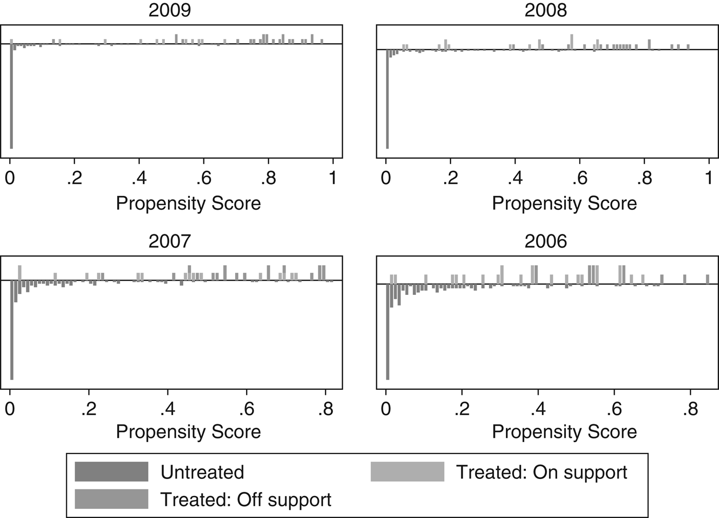
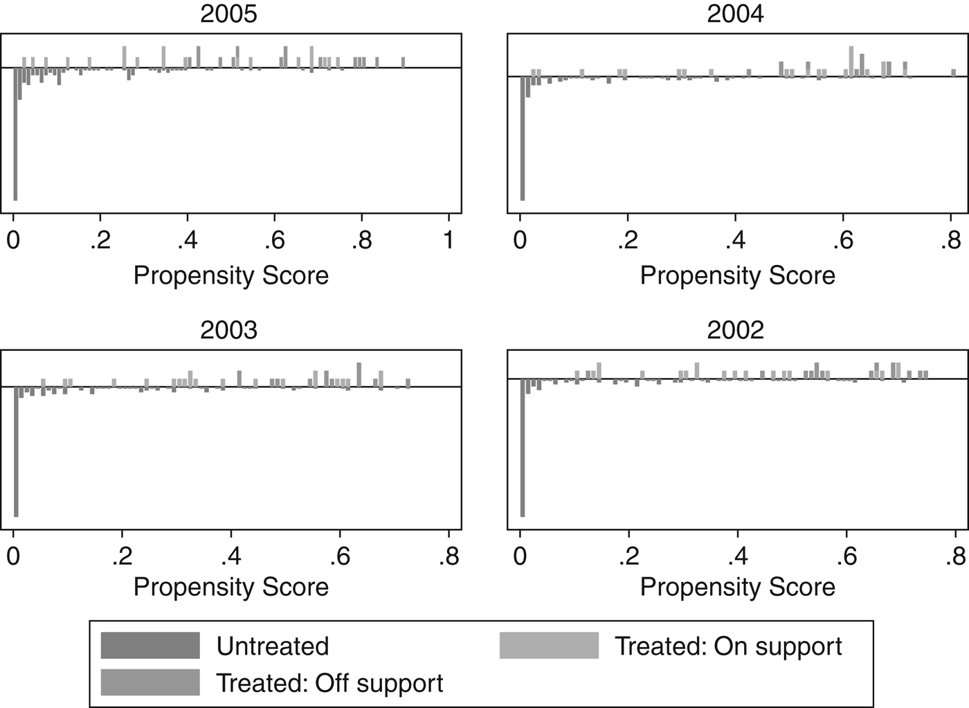
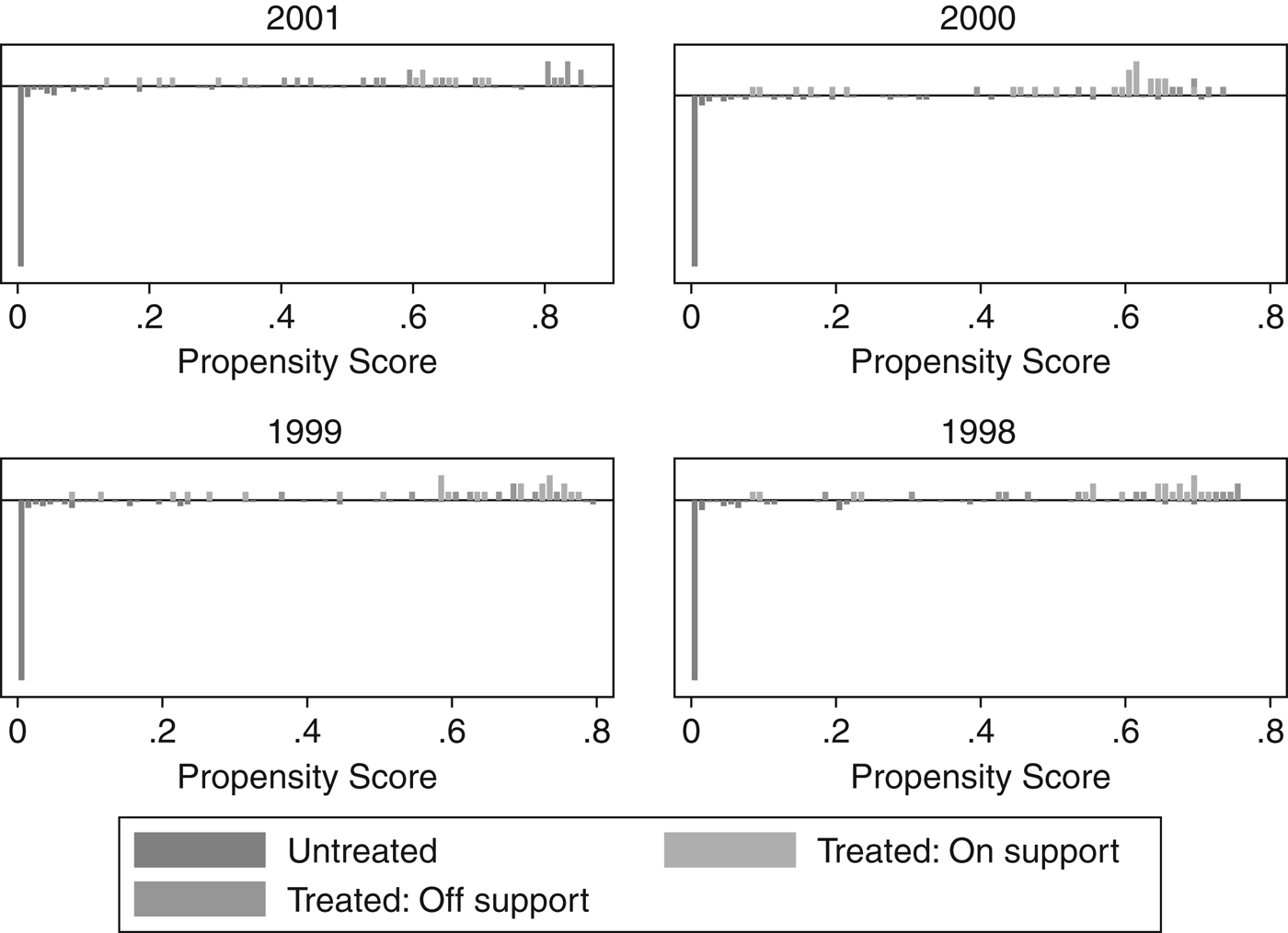
The validity of the ATT is conditioned by the fulfilment of two assumptions. The first assumption, conditional independence, assumes that the selection into treatment is solely based on observable characteristics. We are aware that there could be unobserved variables, which could be correlated with the decision to ratify Kyoto and different from the ones we control for. The second assumption is the common support condition. The common support region includes all the observations where the balancing score has a positive density for both treated and untreated countries. There has to be an overlap between treated and untreated countries in order to match them (Khandker et al., Reference Khandker, Koolwal and Samad2009). We present the results on the density distribution of the propensity scores and the common support region in figures A1–A5 in the appendix.
In order to analyze through which channel the Kyoto commitments have led to declining emissions, we modify the model specification in equation (1) and use the emission intensity, namely the amount of CO2 emissions per unit of GDP, as the dependent variable:
 $$\ln \left(\displaystyle{{CO_{2it}}\over{GDP_{it}}}\right)=\alpha_i\, +\, \lambda_t+ \beta_1 Kyoto_{it} + \beta_2 \ln POP_{it} + \beta_3 \ln GDPH_{it}+\varepsilon_{it}. $$
In this way we analyze how having Kyoto commitments influences countries' emission intensities. Technological change, which is in most cases policy induced, does not cut emissions directly but does have an effect on the emission intensity of each unit of GDP. Our model relegates the factors of economic structure, technology progress and energy mixture to the error term since our focus is on the effect of policies induced by the Kyoto Protocol. Ang (Reference Ang2005) as well as Yang and Chen (Reference Yang and Chen2011) analyze the direct effect of the economic structure, technology and energy mix on emissions.
3.2. Data
CO2 emission data are from the Carbon Dioxide Information Analysis Center (CDIAC, 2012) and include emissions from solid, liquid and gas fuel consumption as well as emissions from cement production and gas flaring. The panel is unbalanced because the data on CO2 emissions for economies in transition are only available from 1992 onwards. Therefore, we restrict our data set to 170 countries over the period 1992–2009 in order to have CO2 emission data for each country and each year.
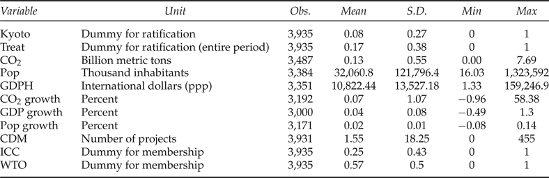
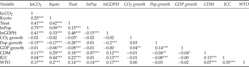
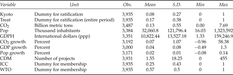
Figure 1 shows that CO2 emissions have steadily increased over the whole period and in all countries. High-income countries emit on average more than 10 times the amount of CO2 over low-income countries. The lower-middle income countries display a more volatile trend and surpass high-income countries in 2008, mainly due to the upturn in emissions from China and India. The data on Kyoto Protocol ratification and CO2 emission reduction commitments are from the UNFCCC (2010) and the data on the number of financed CDM projects per country are from the UNEP Risoe Centre (UNEP, 2012). The data on GDP per capita and population are taken from the Penn World Tables (Heston et al., Reference Heston, Summers and Aten2011). Summary statistics and cross-correlations for the variables used in the analysis are presented in tables A2 and A3 in the appendix.
Average CO2 emissions of high-, middle- and low-income countries

3.3. Main results and policy recommendations
In the first part of this section we present the results obtained using the difference-in-differences estimator with matching and in the second part we discuss how the Kyoto Protocol could have affected emissions.
Table 1 presents the results from the probit regression used to estimate the propensity scores for ratifying Kyoto with emissions commitments. As in equation (3), the dependent variable Treat takes a value of one for the treated units. Out of the three key variables which influence the decision to ratify Kyoto with commitments, only growth in GDP and CO2 emissions are statistically significant.
Results from estimating the propensity scores for ratifying Kyoto with commitments

Notes: The dependent variable is Treat. Robust standard errors are in brackets, ***p < 0.01; **p < 0.05; *p < 0.1.
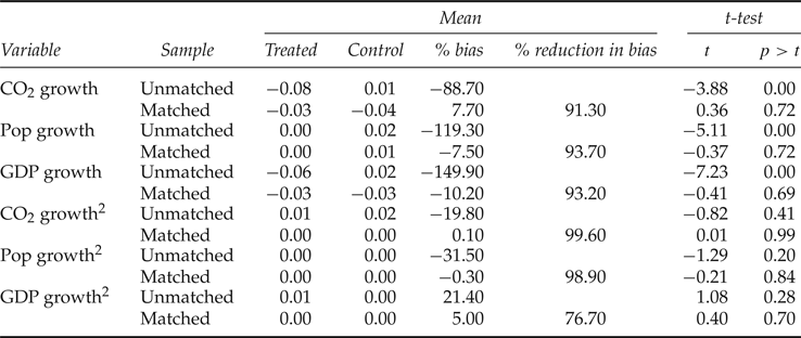
We choose nearest neighbour matching to create the control group by matching countries with commitments (the treated group) to those without commitments and with a similar likelihood of being in the treated group. The quality of the match relies on the balancing property and the test of the difference in means of the independent variables after the match is made. We show that the balancing property is met and the difference in the mean propensity score between the treated and control group is 0.28 points. Table A4 in the appendix shows that there is no significant difference between the treated group and the control group in terms of the means of the explanatory variables, namely GDP per capita and population growth, after matching.
Next we apply a difference-in-differences estimator to calculate the average treatment effect so that we can control for the unobservable country heterogeneity and common time effects that may also affect emissions. Table 2 shows the main results. Column 1 of table 2 presents the results for the whole sample as a benchmark. The estimated coefficient for the Kyoto variable (−0.19) is negative and statistically significant, but its magnitude is considerably high.
Results using the difference-in-differences estimator, 1992–2009
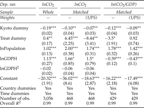
Notes: Robust standard errors are in brackets, ***p < 0.01; **p < 0.05; *p < 0.1. PS, propensity score.
Column 2 presents the same specification estimated using the matched sample instead of the whole sample. An ATT of −0.1 is obtained, indicating that countries that face emission commitments emit on average 10 per cent less CO2 compared to the control group of countries, which have similar characteristics in terms of GDP and population growth, but do not have to cut emissions. It is worth noting that restricting the sample to the matched countries as a way of controlling for the endogeneity of our policy variable indicates that the coefficient is −0.10 (column 2), which points to an upward bias of the coefficient in column 1 (−0.19). In order to refine our estimate and prove its validity, column 3 of table 2 shows the results obtained by using the inverse of the propensity score (PS) as sampling weights. This refinement gives a Kyoto coefficient of −0.07, which is the most conservative estimate and the one we take as most reliable.
Similar to other studies estimating the Kyoto effect, we also conclude that ratifying Kyoto has a negative and significant effect on emissions. In particular, our results show that a country with emission commitments emits on average 7 per cent less CO2 than a country without reduction commitments. This is a lower effect in comparison with the results obtained by Aichele and Felbermayr (Reference Aichele and Felbermayr2012), −8 per cent (estimate from a fixed effects IV regression) and Iwata and Okada (Reference Iwata and Okada2010), who find an effect of about −11 per cent for CO2 emissions (estimate from a fixed effects estimator). Mazzanti and Musolesi (Reference Mazzanti and Musolesi2009) also find the Kyoto Protocol has a negative effect on CO2 emissions for the northern EU country group.
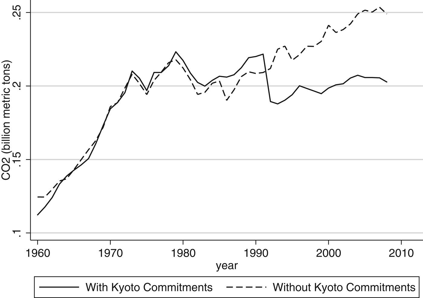
Interestingly, figure 2 indicates that the average emissions of these two country groups mainly diverge from the early 1990s onwards, whereas before that date outcomes moved in tandem, with almost parallel trends. Hence, the existence of similar emissions trends for ‘similar’ countries between the treatment and comparison groups before the policy change validates the use of matching techniques as the preferred model to estimate the Kyoto effect.
Average CO2 emissions of high-income countries only

When turning to columns 4 and 5 in table 2 we find that the estimated Kyoto effect when using emission intensity as the dependent variable yields a slightly larger result. Countries with Kyoto commitments show on average a 9 per cent lower emission intensity per unit of GDP than their comparison group without commitments. This difference in emission intensity could be the channel through which the Kyoto commitments affect countries' emissions. It could be argued that policies such as the Kyoto Protocol induce technological change, which in turn affects emission intensity.
Summarizing, we find that Kyoto countries emit less CO2 than comparable non-Kyoto countries, but the effect is lower than previous studies had estimated. Yet despite the reduced effect, we have been able to find strong indications that the Kyoto Protocol has not failed and that until now it has been the only functioning mechanism to prevent the participating countries from increasing CO2 emissions.
The main policy recommendation derived from this study is that policy makers should actively work towards finding a way of extending the Kyoto Protocol to a wider range of countries, including the so-called new industrialized nations, which indeed should be renamed ‘already’ industrialized countries. Unfortunately, as of 5 December 2014, only 21 countries have ratified the Doha Amendment, which would prolong and renew the commitments from the Kyoto Protocol. The Amendment will only enter into force once three-quarters of the (38) parties to the Kyoto Protocol have deposited their instruments of acceptance.
4. Robustness check
4.1. Pre-Kyoto differences
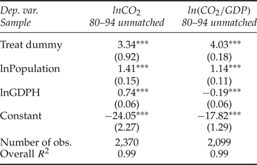
As a robustness check, we run a placebo experiment to test whether the emission-reducing effect from Kyoto is really due to the ratification of the Protocol and not to differences in the initial emission levels between countries. Table 3 shows the results obtained from estimating the same model using the whole sample of countries over the pre-ratification period, more specifically from 1980 to 1994. The Treat dummy takes a value of one for the countries that ratified with commitments at some point in time and zero otherwise. As the coefficient for facing future commitments from Kyoto is statistically significant but positive, we conclude that the Kyoto effect found above is not due to pre-ratification differences in emissions.
Pre-Kyoto estimations

Notes: Robust standard errors are in brackets, ***p < 0.01; *ast; p < 0.05; *p < 0.1.
4.2. IV estimates
Another option to control for endogeneity is to instrument the variable Kyoto with a number of selected instruments. The first proposed instrumental variable is the number of CDM projects financed by public or private entities from the Annex B countries. The CDM, as one of the flexible mechanisms of the Kyoto Protocol, is correlated with the emission reduction commitments of the investing country, but not with its current CO2 emissions. This is because the amount of emissions reduced by the CDM is very small and, even if it did affect a country's emissions, this effect would be on future emissions instead of current ones. Even though it is necessary to ratify the protocol in order to invest in CDM projects, we only exploit the correlation between the two variables.Footnote 5 We also use two additional instruments, namely membership of the WTO and, as in Aichele and Felbermayr (Reference Aichele and Felbermayr2012), membership of the ICC. The instruments must fulfil two conditions. They have to be correlated with the instrumented variable and they must not be correlated with the error term. The first stage of the IV approach is:
 $$\eqalign{Kyoto_{it} = & \alpha_i+ \lambda_t+\beta_1 \ln POP_{it} + \beta_2 \ln GDPH_{it} + \beta_3 \ln GDPH_{it}^{2} \cr & + \beta_4\, CDM_{it} + \beta_5\, WTO_{it} + \beta_6\, ICC_{it} + \upsilon_{it}}\comma \; $$
where Kyoto it takes a value one when a country i has ratified the Kyoto Protocol and faces commitments from the treaty at time t, and zero otherwise. α i and λ t are country- and year-specific effects that control for unobservable country heterogeneity and common time-varying effects that could affect the decision to ratify Kyoto. The instruments are CDM it , WTO it and ICC it . In particular, CDM it accounts for the number of CDM projects in which a country invested in year t. WTO it takes a value of one if a country is a member of the WTO in the specific year and zero otherwise. Similarly, ICC it indicates whether or not a country is a member of the ICC. Finally, υ it is the error term. The second stage of the IV approach is:
 $$\eqalign{\ln CO_{2it} = & \alpha_i + \lambda_t + \beta_1 Kyoto_{it} + \beta_2 \ln POP_{it} + \beta_3 \ln GDPH_{it} \cr & +\beta_4 \ln GDPH_{it}^2+\mu_{it}}\comma \;$$
where lnCO 2it is the natural log of CO2 emissions emitted by country i in year t measured in tonnes. The variable Kyoto it is instrumented with the variables from equation (6) and a maximum of three instruments. μ it is the error term.
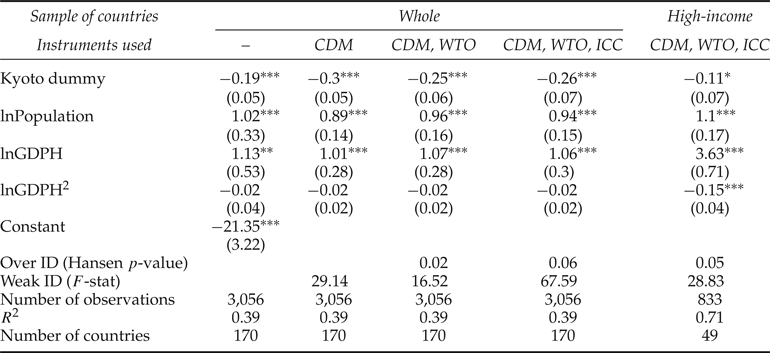
Column 1 in table 4 presents the benchmark regression without instrumenting the Kyoto variable. Column 2 presents the instrumental variable estimation results (−0.3) using the number of CDM projects a country has invested in as the instrument. The Kyoto effect is negative and the magnitude of the effect is even greater than in column 1 but inaccurately estimated. When we add WTO membership as an additional instrument in column 3, the effect declines slightly to −0.25. Nevertheless, the Hansen test rejects the validity of our instruments (p-value = 0.02).
Results from the instrumental variables estimator, 1992–2009

Notes: The dependent variable is lnCO2. Robust standard errors are in brackets, ***p < 0.01; **p <0.05; *p < 0.1. Year dummies are included as regressors.
Similar to Aichele and Felbermayr (Reference Aichele and Felbermayr2012), we add ICC membership as a third instrument. The result hardly changes (−0.26), but the Hansen test still rejects the validity of the instruments. In order to make the sample more homogenous, we reduce the sample to high-income countries in column 5 (table 4). We find that high-income countries with Kyoto commitments emit on average 11 per cent less CO2 than those without commitments. This effect is higher than the result obtained by Aichele and Felbermayr (Reference Aichele and Felbermayr2012), but they use a smaller sample of 40 countries. Apparently, the results are sensitive to small modifications in the sample of countries considered. Indeed, by restricting the sample to ‘similar’ countries, we obtain a more similar Kyoto estimate to the result obtained for the matched sample, but still biased and much larger (0.11 vs. 0.07).
5. Conclusions
This paper tests for an effect of the Kyoto Protocol on CO2 emissions. Our estimates indicate that countries with emission commitments from the Kyoto Protocol emit on average about 7 per cent less CO2 than similar countries that did not ratify the Protocol. We conclude that there is a potential effect from the Kyoto policy on emissions in those countries. The channel of this effect could be the difference in emission intensities between countries with Kyoto commitments and those without. Once a country ratifies the Protocol with emission reduction obligations, it is more likely to pass green growth policies, which do not immediately cut emissions but reduce the emission intensity of GDP. We contribute to the existing literature by using a new identification strategy of the causal effect, namely using matching and difference-in-differences techniques to obtain an accurate estimation of the Kyoto effect.
One matter of concern is whether we can indeed attribute the whole estimated effect to the Kyoto Protocol, as the number of countries that ratified the Protocol and face emission commitments (32) is rather small compared to the number of countries that do not face any emission commitments under the Kyoto Protocol (138). It could be argued that Annex B countries could have put the same effort into reducing their CO2 emissions, even in the absence of the Protocol. Certainly, it is often claimed that regulatory stringency is a positive function of per capita income and in the last decade many developed countries have been taking action to reduce emissions, irrespective of the modest commitments required by the Protocol. In this light, we leave the inclusion of better proxies for regulatory stringency in the model for further research, which will help to support our findings.
In order to stabilize global warming at 2°C, much more serious measures will have to be taken. Although emissions from the developed countries with reduction commitments have declined and some countries like France, the UK and Germany have achieved their targets, the decline in emissions is unlikely to be enough to stabilize levels of GHG in the atmosphere. Emissions from emerging countries, namely China and India, are expected to increase substantially in the near future. Even if the involved developed countries achieve their Kyoto target, it can only be considered a partially successful agreement that is not going to be sufficient to solve the global warming problem. Possible solutions could be to integrate more countries into the treaty, including developing countries, or to establish an international carbon tax on GHG emissions.
As the first commitment round of the Kyoto Protocol has closed in 2012 and as large emission reductions due to the Protocol were observed, it would be desirable for the Doha Amendment, which sets the second commitment round until 2020, to come into practice as soon as possible. Finally, we would like to close the discussion by pointing out that according to our findings even a treaty often seen as a ‘failure’ may in fact be producing some non-negligible effects.
Appendix
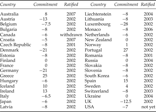
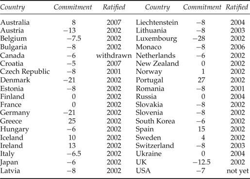
List of Annex B countries with commitments in %
Summary statistics
Cross correlations

Bias reduction after the matching 2009

Region of common support, 2009–2006

Region of common support, 2005–2002

Region of common support, 2001–1998

Region of common support, 1997–1994

Region of common support, 1993–1992