Reservoir Effects

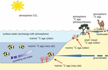
So-called reservoir effects are observed when the reservoir from which an organism derives its carbon differs from the atmosphere ¹⁴C content, necessitating an age-offset correction (see Figure 1). Studies of ¹⁴C activity in the world’s oceans (e.g., Broecker et al. Reference Broecker, Gerard, Ewing and Heezen1960; Bien et al. Reference Bien, Rakestraw and Suess1963) revealed that ocean waters are depleted in ¹⁴C relative to the atmosphere due to slow mixing at the ocean-atmosphere interface, and between surface waters and the deep ocean. For most non-polar regions, the apparent age (“reservoir age”) of the surface layer of the ocean was initially determined to be approximately 400 years, while the reservoir age of the deepest water was in excess of 1000 years (Broecker et al. Reference Broecker, Gerard, Ewing and Heezen1960; Stuiver et al. Reference Stuiver, Pearson and Braziunas1986). Consequently, marine biogenic carbonate samples yield ¹⁴C ages that are older than contemporaneous terrestrial samples (Stuiver and Polach Reference Stuiver and Polach1977; Stuiver et al. Reference Stuiver, Pearson and Braziunas1986). In the late 1960s and early 1970s, two approaches to correcting fossil marine carbonate dates were favored: (1) subtracting the “apparent age” (reservoir age) from the ¹⁴C age measured on the sample, or (2) using modern shells from the same area as the primary standard (Mangerud Reference Mangerud1972). The former method proved more useful because the latter presupposed a series of different geographically specific standards, thereby limiting the comparability of results. Later, ¹⁴C reporting conventions were ratified that standardized the definition of “conventional radiocarbon age.” These specified the reporting of ¹⁴C ages and reporting reservoir age corrections separately from the conventional ¹⁴C age (Stuiver and Polach Reference Stuiver and Polach1977).

Figure 1

Schematic explanation of differences in apparent ages of marine organisms, here on the example of shells, therefore different reservoir ages and reservoir effects respectively. Figure taken from Lindauer (Reference Lindauer2019) dealing with reservoir effects in the Arabian Sea.

Terminology related to ¹⁴C reservoir effects was standardized in the 1980s but can still be a source of confusion. The reservoir age, R(t), is defined as the difference between conventional ¹⁴C ages of samples grown contemporaneously in the atmosphere and the surface ocean (Stuiver et al. Reference Stuiver, Pearson and Braziunas1986). A related parameter is the local reservoir offset, ΔR, which is defined as the local deviation from the global-ocean average reservoir age as represented by the marine ¹⁴C calibration curve. Stuiver and colleagues (Reference Stuiver and Reimer1986) developed the first marine ¹⁴C calibration curve based on a 1-D model of the global ocean. Subsequent refinements to the marine calibration curve have improved accuracy and precision and extended the calibration record deeper in time (Stuiver and Braziunas Reference Stuiver and Braziunas1993; Stuiver et al. Reference Stuiver, Reimer and Braziunas1998; Hughen et al. Reference Hughen, Baillie, Bard, Beck, Bertrand, Blackwell, Buck, Burr, Cutler, Damon and Edwards2004; Reimer et al. Reference Reimer, Baillie, Bard, Bayliss, Beck, Blackwell, Ramsey, Buck, Burr, Edwards, Friedrich, Grootes, Guilderson, Hajdas, Heaton, Hogg, Hughen, Kaiser, Kromer, McCormac, Manning, Reimer, Richards, Southon, Talamo, Turney, van der Plicht and Weyhenmeyer2009, Reference Reimer, Bard, Bayliss, Beck, Blackwell, Bronk Ramsey, Buck, Cheng, Edwards, Friedrich, Grootes, Guilderson, Haflidason, Hajdas, Hatté, Heaton, Hoffman, Hogg, Hughen, Kaiser, Kromer, Manning, Niu, Reimer, Richards, Scott, Southon, Staff, Turney and van der Plicht2013; Heaton et al. Reference Heaton, Köhler, Butzin, Bard, Reimer, Austin, Bronk Ramsey, Grootes, Hughen, Kromer, Reimer, Adkins, Burke, Cook, Olsen and Skinner2020). Prior to the Marine13 curve (Reimer et al. Reference Reimer, Bard, Bayliss, Beck, Blackwell, Bronk Ramsey, Buck, Cheng, Edwards, Friedrich, Grootes, Guilderson, Haflidason, Hajdas, Hatté, Heaton, Hoffman, Hogg, Hughen, Kaiser, Kromer, Manning, Niu, Reimer, Richards, Scott, Southon, Staff, Turney and van der Plicht2013), temporal variations of the global reservoir age were only considered for the period after 13.9 cal kBP. For the period between 13.9 and 10.5 cal kBP the curve was based on foraminifera and coral data, while for the Holocene, an ocean-atmospheric box model (Stuiver and Braziunas Reference Stuiver and Braziunas1993) was used based on the atmospheric curve. For the period between 50 and 13.9 cal kBP R(t) was treated as constant with the value of 405 ± 20 ¹⁴C years.

Differences in coastal geomorphology, ocean circulation, upwelling, and freshwater inputs produce localized deviations from the global-average ocean reservoir age. Corrections for such localized offsets, ΔR, can be estimated by measuring known-age, live-collected marine materials (e.g., museum specimens, samples independently absolutely dated), or for fossil mollusks by using contemporaneous terrestrial and marine sample pairs. Calculating ΔR from the difference in the known calendar age of the marine material and its apparent ¹⁴C age is straightforward arithmetic. To facilitate access to published ΔR values, Reimer and Reimer (Reference Reimer and Reimer2001) developed an online database of published ΔR data derived from known-age, mostly pre-bomb (i.e., pre-1950 AD) shell specimens, accessible via mapping software. Fossil biogenic carbonates that were not live-collected with reservoir effects determined from marine–terrestrial pairs are not included in this database and need to be taken from publications dealing with the respective or nearby locations.

As a first approximation, ΔR was assumed to be a constant for a given region (Stuiver et al. Reference Stuiver, Pearson and Braziunas1986). However, researchers have demonstrated considerable variability over short- and long-term timescales (Austin et al. Reference Austin, Bard, Hunt, Kroon and Peacock1995; Deo et al. Reference Deo, Stone and Stein2004; Culleton et al. Reference Culleton, Kennett, Ingram, Erlandson and Southon2006; Hadden and Schwadron Reference Hadden and Schwadron2019). In the Arabian Sea, for example, ΔR declined by over 400 ¹⁴C yr over the period ca. 6100–3400 ¹⁴C yr BP (Lindauer et al. Reference Lindauer, Santos, Steinhof, Yousif, Phillips, Jasim and Hinderer2017).

To derive temporally specific ΔR values for a particular region, the typical way to estimate ΔR for fossil specimens (e.g., archaeological shells) is to measure the ¹⁴C content of contemporaneous terrestrial and marine samples, for example archaeological shells found in close association with terrestrial material such as wood, charcoal, well-preserved terrestrial animal bone, or, in some cases, suitable terrestrial mollusk shells (Carvalho et al. Reference Carvalho, Macario, Oliveira de, Oliveira, Chanca, Alves, Souza, Aguilera and Douka2015; Macario et al. Reference Macario, Alves, Chanca, Oliveira, Carvalho, Souza, Aguilera, Tenório, Rapagna, Douka and Silva2016). Calculating ΔR involves the calibration of the terrestrial samples, differencing the measured ¹⁴C_marine age from that predicted by the marine model for that calibrated age, and calculating an appropriate estimate of uncertainty. Reimer and Reimer (Reference Reimer and Reimer2017) explain how to obtain ΔR estimates in different scenarios and provide an online tool that facilitates the calculation of such estimates. Ideally, more than one sample pair is available from the same archaeological context (Cook et al. Reference Cook, Ascough, Bonsall, Hamilton, Russell, Sayle, Scott and Bownes2015; Russell et al. Reference Russell, Cook, Ascough, Scott and Dugmore2016). If there is no reason to associate one specific marine sample with one specific terrestrial sample, a multiple-pair approach can be used to provide a more robust ΔR estimate (Russell et al. Reference Russell, Cook, Ascough, Scott and Dugmore2016). This approach considers in pair-wise fashion each marine sample as being associated with each terrestrial sample, giving individual ΔR values for all possible combinations of values. Alves et al. (Reference Alves, Macario, Ascough and Bronk Ramsey2018) estimated local ΔR values for locations and time ranges where no empirical data are available, based on the model developed by Butzin (Reference Butzin, Heaton, Köhler and Lohmann2020) for estimating R(t) over time. Notably, ΔR estimates are calibration curve product specific (Butzin et al. Reference Butzin, Heaton, Köhler and Lohmann2020; Heaton et al. Reference Heaton, Köhler, Butzin, Bard, Reimer, Austin, Bronk Ramsey, Grootes, Hughen, Kromer, Reimer, Adkins, Burke, Cook, Olsen and Skinner2020; Reimer et al. Reference Reimer, Austin, Bard, Bayliss, Blackwell, Bronk Ramsey, Butzin, Cheng, Edwards, Friedrich, Grootes, Guilderson, Hajdas, Heaton, Hogg, Hughen, Kromer, Manning, Muscheler, Palmer, Pearson, van der Plicht, Reimer, Scott, Southon, Turney, Wacker, Adolphi, Büntgen, Capano, Fahrni, Fogtmann-Schulz, Friedrich, Köhler, Kudsk, Miyake, Olsen, Reining, Sakamoto, Sookdeo and Talamo2020). For consistency, literature-based estimates of ΔR need to be updated prior to use.

The methods described above assume ΔR values follow a Gaussian distribution, which can be described in terms of mean and sigma. However, calibrated ages are best represented as probability distributions, rather than point estimates, and these are often asymmetric due to the oscillatory pattern of the calibration curves. Likewise, it may be appropriate to present ΔR estimates as non-Gaussian probability distributions, for example, by means of Bayesian chronological modeling. Macario et al. (Reference Macario, Souza, Aguilera, Carvalho, Oliveira, Alves, Chanca, Silva, Douka, Decco and Trindade2015) used the OxCal software (Bronk Ramsey Reference Bronk Ramsey2009) to model the local reservoir effect ΔR for an archaeological site located on the coast of Rio de Janeiro, Brazil, by modeling contemporary archaeological sample sets as Phases and assuming a uniform prior probability for ΔR. Following Bronk Ramsey and Lee (Reference Bronk Ramsey and Lee2013), ΔR was specified as a uniform probability distribution over an arbitrarily large but plausible range of values. The result is a posterior probability distribution for ΔR that takes into account the prior probability as well as all other model parameters. Here, also species-specific values can be modeled in one run, which is quite convenient. Examples of this application can be found in Hadden and Schwadron (Reference Hadden and Schwadron2019), Lindauer et al. (Reference Lindauer, Santos, Steinhof, Yousif, Phillips, Jasim and Hinderer2017), Macario et al. (Reference Macario, Souza, Aguilera, Carvalho, Oliveira, Alves, Chanca, Silva, Douka, Decco and Trindade2015, Reference Macario, Alves, Chanca, Oliveira, Carvalho, Souza, Aguilera, Tenório, Rapagna, Douka and Silva2016, Reference Macario, Alves, Belém, Aguilera, Bertucci, Tenório, Oliveira, Chanca, Carvalho, Souza, Scheel-Ybert, Nascimento, Dias and Caon2018), Milheira et al. (2017), and Zazzo et al. (Reference Zazzo, Munoz, Badel, Béguier, Genchi and Marcucci2016).

Mollusk Shells

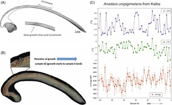
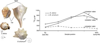
Mollusk shells are usually found in near shore environments, and most often represent coastal and estuarine regimes. They occur either as bivalve shells, such as Anadara uropigimeana (Figure 2), consisting of two halves with the animal inside, or as gastropod shells that have a single valve that spirals about a central axis (Figure 3). Carbon in the mineral phase of the shell is derived primarily from ambient bicarbonate and dissolved inorganic carbon (DIC), and to a lesser extent from diet (McConnaughey and Gillikin Reference McConnaughey and Gillikin2008). Shells were tested in the early stages of the development of the ¹⁴C research, but due to their unexpectedly old ages were once thought of as unreliable materials for ¹⁴C dating (Anderson and Libby Reference Anderson and Libby1951; Olsson Reference Olsson2009). Although significant advances have been made, interpreting ¹⁴C data from mollusk shells remains a challenge due to complex interplay among marine ¹⁴C dynamics, ecological and vital/metabolic effects; idiosyncrasies related to mollusk longevity and shell growth patterns; and contamination/recrystallization effects. These challenges serve to caution coastal archaeologists to critically evaluate the life habits and habitats of target taxa, with special consideration given to the source and isotopic composition of the carbon reservoir from which the animal’s tissues are derived. In particular, they serve to caution against uncritical application of ΔR estimates across taxa, or across large geographic regions. Intrashell variability in ¹⁴C, combined with challenges of correcting for reservoir offsets, can severely limit the effective precision of ¹⁴C age determinations on marine and estuarine shell carbonates (Culleton et al. Reference Culleton, Kennett, Ingram, Erlandson and Southon2006; Lindauer et al. Reference Lindauer, Friedrich, Gyseghem and Hinderer2019).

Figure 2

Description of growth pattern in bivalves: (A) sampling for stable isotopes and high resolution ¹⁴C measurements; (B) sampling of a neolithic Anadara uropigimelana from Kalba, UAE. Measurement results are presented in panel (C) where “DOG” refers to direction of growth. Adapted from Lindauer (Reference Lindauer2019).

Figure 3

Within-shell variability of ¹⁴C content in two species of marine gastropods. Dashed spiral indicates direction of growth, coiling about a central axis. Adapted from Hadden and Cherkinsky (Reference Hadden and Cherkinsky2017).

Carbonate Corals

When one hears the word “coral” most people think of warm weather, tropical waters, and places such as the Great Barrier Reef or the Caribbean. To a ¹⁴C specialist when they hear the world “coral” they picture a unique archive of past ¹⁴C oceanic variations. Carbonate corals, whether from shallow or deep water, record within their skeletons the Δ¹⁴C content of the waters in which they lived and grew (e.g., Knutson and Buddemeir Reference Knutson and Buddemeier1973; Druffel and Linick Reference Druffel and Linick1978; Roark et al. Reference Roark, Guilderson, Flood-Page, Dunbar, Ingram, Fallon and McCulloch2005). Some corals require unturbid, warm, moving water in subtropical and tropical seas such as Hawai´i or Pacific Remote Islands area (shallow corals). But over 50% of the known corals are found in cold, deep and dark waters: i.e., cold water or deep-sea corals. These ahermatypic corals can be found from near the surface to depths of 6000m. The carbonate skeleton of the coral is amenable to not only ¹⁴C analysis but independent Th/U dating (e.g., Thurber et al. Reference Thurber, Broecker, Blanchard and Potratz1965; Adkins et al, Reference Adkins, Griffin, Kashgarian, Cheng, Druffel, Boyle, Edwards and Shen2002) and, at least for reef-building hermatypic corals (reef-building shallow water corals with symbiotic zooxanthellae), sclerochronology and seasonal cycles in stable isotopes and/or metal/calcium ratios for the construction of subannually resolved age-models (e.g., Guilderson et al. Reference Guilderson, Schrag, Kashgarian and Southon1998). Known-age and live-collected specimens are used to (1) reconstruct local to regional surface ocean reservoir ages (e.g., Druffel and Linick Reference Druffel and Linick1978; Goodkin et al. Reference Goodkin, Switzer, McCorry, De Vantier, True, Hughen and Yang2011; Toth et al. Reference Toth, Cheng, Edwards, Ashe and Richey2017), (2) elucidate water mass exchange and mixing in surface waters (e.g., Ramos et al. Reference Ramos, Goodkin, Druffel, Fan and Siringan2019) as well as for the ocean’s interior, particularly during the last deglaciation (e.g., Burke and Robinson Reference Burke and Robinson2012), and (3) further detail marine ¹⁴C-calendar calibration (e.g., Bard et al. Reference Bard, Hamelin, Fairbanks and Zindler1990, Reference Bard, Arnold, Fairbanks and Hamelin1993).

To understand the importance of corals also for the construction of the calibration curve necessary for ¹⁴C dating, a closer look at the early times of ¹⁴C calibration seems appropriate. It was in the 1960s when deVries, Damon, Stuiver, Suess and other radiocarbon pioneers, collaborating with dendrochronologists across the globe, were independently moving beyond the “curve of knowns” (Arnold and Libby Reference Arnold and Libby1949) to reconstruct past variations in atmospheric Δ¹⁴C. Variability in Δ¹⁴C as a function of latitude and time had been documented early on (e.g., de Vries Reference de Vries1958; Suess Reference Suess1960; Willis Reference Willis, Tauber and Münnich1960; Stuiver Reference Stuiver1961; Damon Reference Damon, Long and Grey1966) and it was recognized that conversion of ¹⁴C years to a calendrical timescale would have great impact in archaeological and other communities. The independent calendar calibration curves, using overlapping anchored (and floating) tree-ring sequences, were in their early years, prior to the standardization of reporting (Stuiver and Polach Reference Stuiver and Polach1977), consistent handling of inter-laboratory offsets, and some personal interpretation of the curves’ themselves (e.g., Suess Reference Suess1970). It was, no doubt, some version of geochronology’s “wild west” (see Reimer Reference Reimer2021, this issue). By the mid-1980s a consistently handled, dendrochronlogical record provided a bidecadal calibration curve to 9160 cal yr BP (7210 cal BC–AD 1950: Stuiver and Reimer Reference Stuiver and Reimer1986).

At about the same time as the 1986 calibration publication, two independent but serendipitous things occurred. At the California Institute of Technology, Larry Edwards, with a focus on reef-building hermatypic corals and geologically young carbonate samples, was revamping the methodology for Th/U dating (thorium/uranium dating) of marine carbonates (Edwards et al. Reference Edwards, Chen and Wasserburg1987). On the other side of the United States, Rick Fairbanks at Lamont-Doherty Geological Observatory (now Earth Observatory) was finishing the pre-planning for an expedition to core the ancient, submerged coral reefs off the Oistins coast of Barbados. The intersection of these two events: precise, paired ¹⁴C and Th/U analyses of reef-building corals spanning the last 30,000 years (Fairbanks Reference Fairbanks1989; Bard et al. Reference Bard, Hamelin, Fairbanks and Zindler1990), directly lead to an extension of the calibration timescale (Bard et al. Reference Bard, Arnold, Fairbanks and Hamelin1993; Stuiver and Reimer Reference Stuiver and Reimer1993) and indirectly paved the way for the inclusion of the varved Cariaco Basin (i.e., laminated sediment records from the Cariaco Basin) ¹⁴C surface water reconstruction to be included in IntCal98 (Stuiver et al. Reference Stuiver, Reimer and Braziunas1998). Although the data density of the absolutely dated Barbados coral suite could not match that of the Cariaco varved section, the discrete coral data provided ground-truthing for the varve ages. Moreover, the Barbados results robustly documented, for the first time, a much larger difference between ¹⁴C and absolute ages than previously surmised: the ¹⁴C ages were systematically younger than absolute ages by as much as ∼3.5 ky at the last glacial maximum, 20 ky ago. Subsequent ¹⁴C-calibration studies confirmed these results (e.g., Durand et al. Reference Durand, Deschamps, Bard, Hamelin, Camoin, Thomas, Henderson, Yokoyama and Matsuzaki2013, among many).

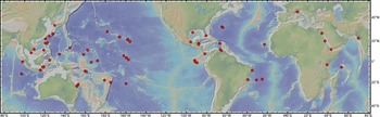
Knutson and Buddemeir (Reference Knutson and Buddemeier1973) were likely the first to measure ¹⁴C in living coral and seawater from a lagoon at Fanning Island. By the end of the decade the first of many coral-based Δ¹⁴C surface water time series were published (Druffel and Linick Reference Druffel and Linick1978; Nozaki et al. Reference Nozaki, Rye, Turekian and Dodge1978). These early records were by technical necessity, annual or biannual in resolution and documented surface water Δ¹⁴C leading up to and through the atmospheric weapons testing era. The advent of accelerator-based ¹⁴C measurements (e.g., Nelson et al. Reference Nelson, Korteling and Stott1977) significantly reduced sample mass and preparation requirements. In the intervening decades there has been a profusion of shallow water pre/post-bomb Δ¹⁴C reconstructions, many with subannual resolution (Figure 4).

Figure 4

Global distribution of pre- to post-bomb coral-based surface water reconstructions published in the literature. Many of these records have subannual resolution.

For studying shallow ocean processes, coral records from the Pacific, South China Sea, and Indonesian Seas are some of the best documented. In a simplified sense, in the Pacific there exists an oceanic Hadley cell (circulation cell) where subduction occurs in the subtropics and extra-tropics and this water ventilates the tropical thermocline (transition layer between warmer mixed water at the ocean´s surface and the cooler waters below) where it upwells and returns to the subducting regions through wind-driven surface flow (e.g., Wyrtki and Kilonsky Reference Wyrtki and Kilonsky1984). Surface water exits the western tropical Pacific into the Indian Ocean through the Indonesian Seas either directly or via mixing within the South China Sea (Qiu et al. Reference Qiu, Mao and Kashino1999). Tritium and ³He tracer data indicate that the ventilation time-scale (time it takes to bring fresh surface waters into the ocean interior) of the tropical thermocline is on the order of decades (Fine et al. Reference Fine, Maillet, Sullivan and Willey2001). Significant interior pycnocline (boundary separating layers of different densities) exchange occurs between the subtropics and tropical thermocline and this dynamic process sets up the pan-Pacific surface water ¹⁴C gradient, both “natural” and in the post-bomb era (Toggweiler et al. Reference Toggweiler, Druffel, Key and Galbraith2019, and references therein). Building on the early work of Toggweiler and Trumbore (Reference Toggweiler and Trumbore1985), Fallon and Guilderson (Reference Fallon and Guilderson2008) documented one of the first bomb-¹⁴C surface water transients, associated with nuclear testing in 1954, exiting the Pacific through the Indonesian Seaway and into the Indian Ocean. Subsequent studies have gone to the testing grounds to ascertain the impact of close-in fall-out and production (e.g., Fallon and Norman Reference Fallon and Norman2012).

Pacific Δ¹⁴C reconstructions document the interannual redistribution of surface waters associated with El Niño (e.g., Guilderson et al. Reference Guilderson, Schrag, Kashgarian and Southon1998) and seasonal changes in Δ¹⁴C in the Galapagos Islands reflecting the source of waters being upwelled (e.g., Druffel et al. Reference Druffel, Griffin, Vetter, Dunbar and Mucciarone2014). The visual “jump” observed in ¹⁴C in the 1976 upwelling season in the Galapagos Islands is not simply a reflection of the penetration and arrival of bomb-¹⁴C but due to changes in the source of the waters feeding the upwelling (Guilderson and Schrag Reference Guilderson and Schrag1998). This abrupt change was coincident with a change in the intensity and frequency of El Niño events as a response to the large-scale wind-field and the 1976 climate shift related to a change in the Pacific Decadal Oscillation. In the North Pacific Subtropical Gyre, there are inflection points on the post-bomb decrease that coincide with moderate to strong La Niñas following moderate to strong El Ninos (Guilderson et al. Reference Guilderson, Schrag, Druffel and Reimer2021) when upwelling in the eastern Pacific can be more intense and entrain more or deeper, lower ¹⁴C waters.

Smoothing/averaging in the time domain in post-bomb era coral-based reconstructions may be a boon relative to discrete, instantaneous sampling of the surface mixed layer. Analyses of discrete water samples can have a representation bias at the 10–20‰ level, well beyond analytical reproducibility (e.g., McDuffee and Druffel Reference McDuffee and Druffel2007; Druffel and Griffin Reference Druffel and Griffin2008). One can surmise that if the chronology is accurate and precise, coral (and other reliable bioarchive) based reconstructions of surface water Δ¹⁴C could be more amenable to ocean model experiments and data-model comparisons. Methodical data-model comparisons require a reliable and well-documented age-model for the Δ¹⁴C time series. If a record is off by one year it does not make much difference in the pre/post-bomb peak assessment and implications on air-sea ¹⁴CO₂ exchange. However, poor chronologies will make a mess of exploring the evolution of water masses and mixing processes. To fully exploit the small natural (i.e., pre-bomb) ¹⁴C gradients requires high accuracy and precision, and replication to confirm representativeness of individual records.

One of the most intriguing application of ¹⁴C analysis in carbonate corals is the ability to reconstruct past Δ¹⁴C of the interior ocean (e.g., Adkins et al. Reference Adkins, Griffin, Kashgarian, Cheng, Druffel, Boyle, Edwards and Shen2002; Burke and Robinson Reference Burke and Robinson2012). Unlike planktic-benthic foraminifera analyses, we can independently, place the deep-sea coral Δ¹⁴C on an absolute timescale with Th/U. Not needing to go through planktonic foraminfera ¹⁴C to a calibrated age or e.g., a wiggle match to an ice core isotope record is extremely powerful in independently elucidating the timing of Δ¹⁴C changes in the interior ocean’s carbon reservoirs and teasing apart the mechanisms of how the ocean moved between a glacial and modern circulation state with subsequent cascades into the larger earth system. However, although they are ubiquitous in the deep-sea, we do not find deep-sea corals everywhere as they do not occur everywhere. They usually require a hard substrate to attach to and, like their shallow water cousins, do not thrive in turbid, sediment rich, locations. They are mainly found on exposed hard grounds, including in canyons, and seamounts. In terms of paleo-reconstructions, seamounts and lithoherms (deep-water reefs) of the North Atlantic and parts of the current scoured Southern Ocean have been particularly fruitful to look for ancient deep-sea corals (Robinson et al. Reference Robinson, Adkins, Keigwin, Southon, Fernandez, Wang and Scheirer2005). The Pacific basin, due to its low carbonate ion content, is much less forgiving to carbonate material on the seafloor: over millennia it can dissolve away. The spatial bias inherent in this potentially unique archive needs to be explored in a more systematic manner. Where we do have both benthic foraminifera and deep-sea coral data (e.g., Robinson et al. Reference Robinson, Adkins, Keigwin, Southon, Fernandez, Wang and Scheirer2005) it can be difficult to reconcile the differences in the data (e.g., Zhao et al. Reference Zhao, Marchal, Keigwin, Amrhein and Gebbie2018). Deep-sea coral data more often has better temporal resolution resulting in higher amplitude Δ¹⁴C variations than that observed in pooled foraminifera data which often integrates 10s to 100s of years.

Particularly large Δ¹⁴C variations are observed in intermediate and deep-waters which exceed that of the reconstructed atmospheric Δ¹⁴C curve (e.g., Burke and Robinson Reference Burke and Robinson2012; Robinson et al. Reference Robinson, Adkins, Keigwin, Southon, Fernandez, Wang and Scheirer2005). In deep-sea coral samples we may independently discern actual lead/lags of proxies (tracers such as in-situ Δ¹⁴C) which imply a mechanistic process and assess the lead/lag with that imparted by the (deep-ocean) equilibration time of the tracer itself. As discrete samples which individually span a few hundred years, and although they record significant ocean Δ¹⁴C changes that are not contemporaneous with changes in atmospheric Δ¹⁴C, these records pose interpretation challenges to clearly elucidate the ocean circulation component of their Δ¹⁴C signal. A challenge to placing these Δ¹⁴C records in strict paleo-ventilation terms, and the implied mechanistic interpretation, is an accurate and precise knowledge of what the surface water Δ¹⁴C was at the time the deep waters were removed from the surface (e.g., Zhao et al. Reference Zhao, Marchal, Keigwin, Amrhein and Gebbie2018). Like many paleo-tracers (e.g., benthic foraminifer δ¹³C, Cd/Ca, etc.) quantitative interpretations of interior Δ¹⁴C observations still escape the community. This is regardless of potential complications such as low-¹⁴C hydrothermal seeps and plumes resulting from changes in deep-sea volcanism as ice sheets wax and wane (Zhao et al. Reference Zhao, Marchal, Keigwin, Amrhein and Gebbie2018). Until we have reliable, and precise high latitude reservoir ages across the most recent deglacial to provide explicit boundaries for deep water Δ¹⁴C reconstructions, the full potential of deep-sea coral (and benthic foraminifer) Δ¹⁴C as a quantitative ventilation tracer will remain obfuscated.

Other Marine Carbonates: Foraminifera

Although here we concentrated on shells and corals, many more carbonate-building taxa inhabit the oceans that must not be neglected. These include foraminifera (“forams”), some marine algae (e.g., calcareous algae), sclerosponges, bioapatite in the bones of marine vertebrates, and otoliths (“ear stones”) of fishes. Biogenic carbonate structures other than marine shells have been used for derivation of ΔR values, such as fish bone from archaeological sites (Russell et al. Reference Russell, Cook, Ascough and Barrett2011; Alves et al. Reference Alves, Macario, Souza, Aguilera, Goulart, Scheel-Ybert, Bachelet, Carvalho, Oliveira and Douka2015; Macario et al. Reference Macario, Alves, Belém, Aguilera, Bertucci, Tenório, Oliveira, Chanca, Carvalho, Souza, Scheel-Ybert, Nascimento, Dias and Caon2018) and known-age fossil algae (Sanja Faivre et al. Reference Sanja Faivre, Bakran-Petricioli, Barešić and Horvatinčić2014). While these may be representative for a given species and time period, maybe for a location if the organism is stationary, they are not necessarily representative of the marine ¹⁴C conditions in general.

Foraminifera are tiny organisms that can inhabit the sea floor (benthic foraminifera) or float near the surface (planktonic foraminifera), and therefore incorporate carbon of different origin. Planktonic foraminifera float near the surface where they incorporate a mixture of atmospheric and marine ¹⁴C, whereas the larger group of benthic foraminifera remains on the seafloor in depths of up to 4 km, recording a reservoir of older carbon brought down to these depths through ocean circulation. When using both groups and comparing them it can be possible to estimate an apparent ventilation age (Broecker et al. Reference Broecker, Mix, Andree and Oeschger1984; Broecker Reference Broecker2009). With the expansion of accelerator mass spectrometry (AMS) in the early 1980s, a profusion of ¹⁴C dating occurred. Forty years later, we are still trying to resolve questions raised from then. Bioturbation, or physical mixing of sediments, continues to be a challenge in low and even high sedimentation-rate sediments (Peng and Broecker Reference Peng and Broecker1984; Keigwin and Guilderson Reference Keigwin and Guilderson2009, among many). Another somewhat related problem is dissolution-induced breakage leading to a lack of whole planktonic tests below the carbonate lysocline. There are still unresolved questions on the “cleanliness” of foraminifera tests from certain depositional environments, and the “best” way to clean and treat samples prior to analysis. Fine grained detrital carbonate which is not always removed via sonication of whole tests in methanol, the standard cleaning technique, can contaminate results. Physical cracking and inspection of individual test fragments prior to and post sonication is one sparingly used method to deal with detrital carbonate contamination. Using AMS, monospecific samples can be measured to answer, for example, the following two questions: (1) the timing of major temperature changes and meltwater input as well as (2) reconstruction of past changes of the ventilation rate of CO₂ in the oceans (Duplessy et al. Reference Duplessy, Arnold, Bard, Labeyrie, Duprat and Moyes1992).