

With the advent of Optimality Theory (Prince & Smolensky Reference Prince and Smolensky1993), there has been a revived interest in articulatorily and perceptually driven markedness in phonological research. The cross-linguistic prevalence of such markedness relations is indication to some researchers that synchronic phonological grammar should include phonetic details (e.g. Boersma Reference Boersma1998, Steriade Reference Steriade1999, Kirchner Reference Kirchner2000, Flemming Reference Flemming2001, Zhang Reference Zhang2002). However, there are at least two distinct ways in which phonetics can be incorporated in an optimality-theoretic grammar: while Boersma, Steriade, Kirchner and Zhang adhere to the traditional practice of constraint domination by using universal rankings within constraint families, Flemming (Reference Flemming2001) proposes that the costs of constraint violations should be weighted and summed.
I formally compare the predictions of constraint weighting and constraint domination in this paper and argue that constraint weighting is unnecessary as an innovation in Optimality Theory. The arguments are twofold. First, using constraint families with intrinsic rankings, constraint domination formally predicts the same range of phonological realisations as constraint weighting. Second, with proper constraint definitions and rankings, both the additive effect and the locus effect predicted by constraint weighting can be replicated in constraint domination. I also point out two minor calculation errors in Flemming (Reference Flemming2001).
1 The Flemming model
The traditional assumption for phonological representations is that they should only include features that can be used contrastively in some language, and the details of phonetic implementation are the consequence of universal principles (Chomsky & Halle Reference Chomsky and Halle1968). The discovery of language-specificness in phonetic patterns such as coarticulation (e.g. Keating Reference Keating and Fromkin1985, Reference Keating1990, Manuel Reference Manuel1990, Flemming Reference Flemming, Miglio and Morén1997) put phonologists in a dilemma: either the phonological component in the grammar needs to be augmented to include phonetic details or an additional phonetic component needs to be added to the grammar. Although many researchers, including Keating (Reference Keating and Fromkin1985, Reference Keating1990), Pierrehumbert & Beckman (Reference Pierrehumbert and Beckman1988), Pierrehumbert (Reference Pierrehumbert1990, Reference Pierrehumbert1991), Cohn (Reference Cohn1993) and Zsiga (Reference Zsiga1997), have opted for the latter, other researchers have argued that phonetic knowledge is part of linguistic knowledge proper and should be encoded in the phonological grammar, either directly (Boersma Reference Boersma1998, Steriade Reference Steriade1999, Kirchner Reference Kirchner2000, Flemming Reference Flemming2001, Zhang Reference Zhang2002) or mediated via the lexicon (Pierrehumbert Reference Pierrehumbert2000, Reference Pierrehumbert, Bybee and Hopper2001, Reference Pierrehumbert, Gussenhoven and Warner2002).Footnote 1
Flemming (Reference Flemming2001) makes a significant contribution to this debate by not only presenting arguments for the phonetics-in-phonology approach, for example, the parallel behaviour between phonological and phonetic phenomena and the desire to avoid duplicating sound representations at two different levels, but also proposing an explicit model that provides a unified analysis for parallel phonological and phonetic phenomena such as neutralising assimilation and gradient coarticulation. I review his model below.
1.1 Non-neutralising assimilation
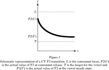
Flemming uses consonant–vowel assimilation in F2 to illustrate the model. He considers a CV sequence in which the F2 targets for the consonant and the vowel are L and T respectively, and the actual realisation of F2 is F2(C) at consonant release and F2(V) at the vowel steady state. The formant transition is schematised in Fig. 1 (from Flemming Reference Flemming2001: 17). The actual realisations F2(C) and F2(V) reflect the compromise between faithful renditions of the consonant locus and vowel target and the least effortful transition between the consonant and the vowel. Flemming formulates three constraints: Ident(C), Ident(V) and MinimiseEffort (MinEffort), whose requirements and costs of violation are defined as in (1) (Flemming Reference Flemming2001: 19).
(1) Constraints for consonant–vowel F2 transitions


Schematic representation of a CV F2 transition. L is the consonant locus, F2(C) is the actual value of F2 at consonant release, T is the target for the vowel and F2(V) is the actual value of F2 at the vowel steady state.

Intuitively, Ident(C) requires the actual realisation of F2 at consonant release to be identical to the consonant locus, and Ident(V) requires the target F2 of the vowel to be reached at the vowel steady state. MinEffort, on the other hand, requires zero transition between the consonant and vowel F2 realisations. These constraints are not ‘ranked’ to predict the output of the grammar. Instead, each constraint is associated with a ‘cost of violation’; e.g. the cost of violation of Ident(C) is the square of the difference between F2(C) and L, weighted by a coefficient w c. The grammar, consequently, is constructed to achieve the least overall cost of violation, which is the sum of the cost of violation for each constraint, as shown in (2) (Flemming Reference Flemming2001: 20).
(2)

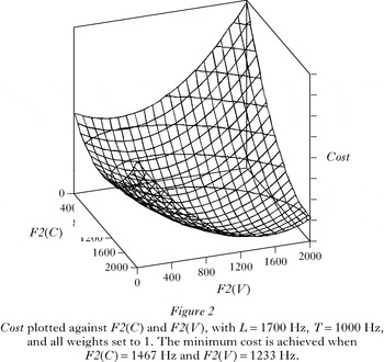
To visualise the effect of F2(C) and F2(V) on the overall cost, Flemming provides a three-dimensional graph in which the x, y and z axes represent F2(C), F2(V) and Cost respectively, as in Fig. 2 (Flemming Reference Flemming2001: 21).
Cost plotted against F2(C) and F2(V), with L=1700 Hz, T=1000 Hz, and all weights set to 1. The minimum cost is achieved when F2(C)=1467 Hz and F2(V)=1233 Hz.

To derive the F2(C) and F2(V) values that render the minimum cost, we take the partial derivatives of Cost along each dimension, which gives rise to two formulas with respect to F2(C) and F2(V), as shown in (3).
(3)
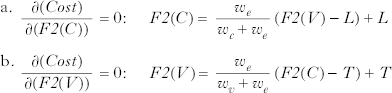
The values of F2(C) and F2(V) obtained from the two formulas in (3) are shown in (4).Footnote 2
(4)
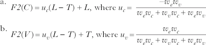
This model can predict the cross-linguistic variability of consonant to vowel coarticulation by adjusting the weight coefficients. For example, the greater the w v value, the more vowel undershoot will contribute to the overall cost; thus it is more important to keep the vowel undershoot small. Such cross-linguistic variability is empirically attested in Flemming's (Reference Flemming, Miglio and Morén1997, Reference Flemming2001) phonetic studies of /u/ undershoot between coronals in four languages.
1.2 Neutralisation
To capture neutralising processes that have phonetic bases and their non-neutralising parallels, the model above is supplemented with constraints on contrasts in the forms of MinDist=Δ and MaximiseContrasts (MaxContrasts), with the former requiring contrastive entities to be of a minimum perceptual distance, and the latter awarding extra contrasts maintained with negative cost values. The categorical nature of neutralising processes is then the result of a cost calculation in which the advantage afforded by keeping a contrast (negative MaxContrasts cost) is outweighed by the cost induced by it (positive MinDist=Δ and MinEffort costs).
Flemming again illustrates the addition to the model with consonant–vowel assimilation, specifically the F2 realisation of /u/ in the context of a coronal and the possibility of neutralising /u/ with /y/. He considers the following constraints.
(5) Constraints for consonant–vowel F2 transitions, with possibility of neutralisation

In this model, MinDist and MaxContrasts are used in lieu of Ident(V), so that the vowel is directly constrained by its difference from contrasting vowels rather than by a specific target. Along the same line, the constraint Ident(C) should only be considered a stand-in for contrast constraints that will yield the F2(t) value when interacting with MinEffort.Footnote 3MinDist=Δ is only violated when the absolute difference between F2(y) and F2(u) is less than Δ, and the cost of violation is proportional to the square of the necessary difference to reach Δ.
MaxContrasts deducts w n from the cost when the /u/~/y/ contrast is maintained. The contrast will only be worth maintaining if the cost that results from keeping the /tu/ syllable is less than w n – in other words, the Cost value as shown in (6) is greater than zero. Otherwise, the grammar will choose to neutralise the /tu/~/ty/ contrast, as the non-existent /tu/ by definition contributes zero to the overall cost.
(6)

To derive the F2(t) and F2(u) values that render the smallest overall cost, we take the partial derivatives of Cost with respect to F2(t) and F2(u) respectively, as in (7).
(7)

The values of F2(t) and F2(u) obtained from the two formulas in (7) are shown in (8).
(8)
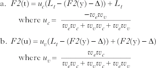
Notice the parallel between (4) and (8): if we replace L with L t and T with F2(y)−Δ in (4), we get exactly (8). Intuitively, the F2 target for /u/ can be construed as F2(y)−Δ, as this is the optimal outcome perceptually – the MinDist violation it incurs is zero. Any F2 value further away from F2(y) will be no better perceptually in terms of how MinDist violation is calculated, but will be undesirable articulatorily.
To illustrate how the model predicts neutralisation with a concrete example, Flemming considers the /u/~/y/ contrast in the /t_t/ context, and makes the following simplifying assumptions:
(9)

Given that the vowel is flanked between two coronals, the cost of violation for MinEffort should be doubled to 2w e(F2(t)−F2(u))2, as there are two CV transitions, and the Ident(C) violation should also be doubled to 2w c(F2(t)−L t)2, as there are two consonants. If we still use (8) to calculate F2(t) and F2(u), we need to double the w c and w e values. The calculation yields an F2(t) value of 1733 Hz and an F2(u) value of 1367 Hz, which consequently give an overall positive cost of 201,667 (the first three items in (6)). Since the benefit of having the contrast is only 200,000, the contrast is not worth maintaining, and /tut/ must be neutralised to /tyt/.
If we adjust the weight values to w c=0·2, w e=0·25 and w v=0·55, then the optimal F2(t) and F2(u) become 1665 Hz and 1317 Hz respectively, and the cost of maintaining the contrast goes down to 191,511. It is then worth keeping the contrast, as the cost is smaller than the benefit. If the vowel is not flanked between two coronals, but only adjacent to one (/tu/~/ty/), the same w c=0·25, w e=0·25, w v=0·5 assumption returns optimal F2(t) and F2(u) values as 1660 Hz and 1220 Hz, which give an overall cost of 121,000 – considerably lower than the threshold of 200,000. This means that the /tu/~/ty/ contrast will be preserved. Flemming's calculation for this case (Flemming Reference Flemming2001: 28), which shows an overall cost of 117,097, is incorrect, I believe. But it does not affect the conclusion that the /u/~/y/ contrast needs to be preserved in the /t_/context.Footnote 4
1.3 Summary
Flemming's model differs from a traditional optimality-theoretic grammar in two important aspects. First, its constraints refer to phonetically detailed representations rather than only representations that are contrastive in some language; consequently, the model also needs constraints that govern the well-formedness of contrasts so that phonetically minute differences do not emerge as contrastive even though they are represented in the grammar. Second, the constraints in the model are associated with weighted costs and the output of the grammar is the phonetic values that incur the least overall cost of all the constraints. In other words, the harmonic value of an output candidate is not defined by its satisfaction of a ranked constraint hierarchy, but by the weighted sum of the costs associated with each constraint. It is this second innovation that I claim to be unnecessary.
Flemming presents two arguments in favour of constraint weighting as a computationally more feasible alternative to constraint domination. First, in order to capture the trade-off relationship between effort and distinctiveness in constraint domination, the constraints need to be split into a great many ranked sub-constraints, and a very particular ranking of these constraints is needed to derive the observed linear relationship between effort minimisation and contrast distinctiveness. Second, the trade-off between effort and distinctiveness constraints is additive; for example, better vowel distinctiveness together with better consonant distinctiveness can motivate more effort expenditure, even though neither distinctiveness is sufficient by itself. To capture all the acceptable trade-offs in constraint domination would require a great many locally conjoined constraints, which would complicate the system too much.
In what follows, I formally compare the predictions of constraint domination with those of constraint weighting by using the same examples as Flemming (Reference Flemming2001) – non-neutralising and neutralising consonant–vowel F2 assimilations, and I show that any single output predicted by constraint weighting can also be predicted by constraint domination, and vice versa. I also show that with proper constraint definitions and rankings, both the additive effect and the locus effect predicted by constraint weighting can also be replicated in constraint domination. Therefore, I argue that constraint weighting is not a necessary innovation in the architecture of Optimality Theory.
Two caveats should be noted upfront. First, the main thesis of Flemming (Reference Flemming2001) is the unification of the treatment of scalar and categorical sound patterns – a point that I do not dispute. My disagreement with Flemming (Reference Flemming2001) is on the technical point of how this unification should proceed – via constraint weighting or constraint domination. Second, Flemming in fact acknowledges that the difference between constraint weighting and constraint domination is considerably narrowed by devices such as constraint decomposition and conjunction, and that there remains the possibility that the constraint system is a mixture of weighting and domination relations, with the latter being reserved for patterns that do not revolve around principles of articulatory ease and perceptual distinctness, such as stress. This further narrows the disagreement between Flemming (Reference Flemming2001) and the current paper.
2 A formal comparison between constraint weighting and constraint domination
2.1 Non-neutralising assimilation
2.1.1 Predictions of the constraint-weighting model
Let us first consider the realm of possible solutions to F2(C) and F2(V) in Flemming's model for non-neutralising assimilation. The F2(C) and F2(V) values that render the minimum cost are given in (4) above. Since L>T, and the phenomenon being captured is F2 coarticulation, F2(C) and F2(V) should meet the condition in (10). This condition can be directly observed from the values of F2(C) and F2(V) in (4): since u c is a negative value and L is greater than T, we deduce that F2(C)⩽L; since u v is a positive value and L is greater than T, we deduce that F2(V)≥T; and since F2(C)−F2(V) is equal to (1+u c−u v)(L−T), which is in turn equal to (w vw c/w ew c+ w vw c+w ew v)/L−T), we deduce that F2(C)≥F2(V).
(10)

Moreover, for any F2(C)~F2(V) pair that satisfies the condition in (10), I show below that it can be a predicted winner in the grammar under certain w e, w c and w v. Since w e, w c and w v are relative weights, we may set one of them to 1 and solve the other two values from the two equations in (4). If we assume that w e=1, we can then derive the values w c and w v as in (11).
(11)

Provided that the condition in (10) is met, we deduce that w c≥0, w v⩽0, indicating that they are both likely weight units for consonant and vowel undershoots. In other words, for any F2(C)~F2(V) pair that satisfies the condition in (10), there exists a grammar that predicts it as the winner.
2.1.2 Predictions of the constraint-domination model
Let us now consider the predictions of constraint domination with ranked sub-constraints in a constraint family.
I also employ Ident(C), Ident(V) and MinEffort, but not as constraints that return costs of violation, but as constraint families with universally ranked sub-constraints.
In (12) I define two Differential Limen Scales with respect to a frequency target F:
(12) Differential Limen Scales

The perceptual steps of an arbitrary frequency from F are defined in (13):
(13) Perceptual steps

Let us again assume that the locus of consonant F2 is L, the target of vowel F2 is T, and L>T. Then the Ident(C) and Ident(V) constraint families can be defined as follows:
(14) Faithfulness constraints
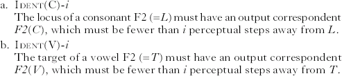
The two families of faithfulness constraints have the following universal rankings:
(15) Universal rankings

These universal rankings stem from the intuition that a perceptually less accurate rendition of the input is a worse violation of faithfulness. They are parallel to assigning a greater cost to a less accurate realisation of the target in Flemming's model. For a formalisation of this intuition as universally ranked constraints in Optimality Theory, see Steriade (to appear).Footnote 5
Let us note that the basic architecture of constraint domination with families of intrinsically ranked constraints in fact allows the continua of phonetics to be modelled to any accuracy we desire. The above discretisation, based on differential limens, is a possible way to keep the numbers of constraints finite, but is not crucial to the architecture of constraint domination itself.Footnote 6
To define the MinEffort constraints, I first define an articulatorily based FrequencyDifference Scale, as in (16).
(16) Articulatorily based Frequency Di‰erence Scale

Assuming that across the F2 range relevant for speech, the effort expenditure associated with F2 is solely determined by the frequency difference, i.e. the effort for F2 to go from 1600 Hz to 1300 Hz is the same as that from 1400 Hz to 1100 Hz, the MinEffort constraint family can then be defined as in (17a), with its universal ranking shown in (17b).
(17) Markedness constraints

Given that research on incomplete neutralisation and the acquisition of second language phonetics has shown that many articulatorily implementable differences cannot be reliably perceived, we can reasonably assume that the Frequency Difference Scale is more finely grained than the Differential Limen Scales. Again, the categorical definition of MinEffort based on the Frequency Difference Scale is only a possible move to keep the number of MinEffort constraints finite. Neither the structure of the constraint family itself nor the results obtained later in the paper depend on the particular numbers of the scale.
It can be proven that under constraint domination, any F2(C)~F2(V) pair that can be predicted by the grammar must also satisfy the condition T⩽F2(V)⩽F2(C)⩽L. The proof can proceed as follows: consider all situations that do not satisfy the above conditions, e.g. T⩽F2(V)⩽L⩽F2(C), T⩽L⩽F2(V)⩽F2(C), etc., and show that there is an alternative that satisfies the condition and is more harmonic with respect to the constraint hierarchy, in other words, any candidate for which (a) either F2(C) or F2(V) falls outside the range (T, L) or (b) F2(V)>F2(C) is harmonically bounded by a candidate that satisfies T⩽F2(V)⩽F2(C)⩽L. For reasons of space, I consider this condition as a given.
Let us assume that L and T are n perceptual steps away from each other. In what follows, under the assumption that the Frequency Difference Scale is more finely grained than the Differential Limen Scales, I show that for any i and j between 0 and n and i+j⩽n, there is a F2(C)~F2(V) pair such that F2(C) is i perceptual steps away from L and F2(V) is j perceptual steps away from T which can be predicted as the winner by the grammar under some ranking. In so doing, I show that constraint domination and constraint weighting predict the same range of single outputs for non-neutralising assimilation, namely T⩽F2(V)⩽F2(C)⩽L, and should thus be considered formally equivalent in this regard.
Consider any i and j such that 0⩽i, j⩽n and i+j⩽n. For all the F2(C)~F2(V) pairs such that F2(C) is i perceptual steps away from L and F2(V) is j perceptual steps away from T, we can calculate all the F2(C)−F2(V) values, which may fall in different ranges along the Frequency Differences Scale. We can then pick any F2(C)~F2(V) pair that falls in the lowest range, which we assume to be (Δf k, Δf k+1) (therefore Δf k⩽F2(C)−F2(V)<Δf k+1), and the constraint ranking in (18) will predict this F2(C)~F2(V) pair as the winner. We assume that Δf m⩽L−T<Δf m+1; thus the highest relevant MinEffort constraint in (18) is MinEffort−Δf m.
(18)
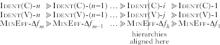
The equal ranking of the three constraints Ident(C)-i, Ident(V)-j and MinEffort-Δf k on the hierarchy, as shown in (18), is crucial. F2(C)~F2(V) as it stands violates all three constraints: F2(C) and F2(V) are i and j perceptual steps from their targets respectively, but Ident(C)-i and Ident(V)-j require the F2 realisations of consonant and the vowel to be fewer than i and j perceptual steps from their targets respectively (see (14)); F2(C)−F2(V)≥Δf k, but MinEffort-Δf k requires their difference to be less than Δf k (see (17)). But a smaller F2(C), which is perceptually further away from L, will violate a higher-ranked Ident(C) constraint; a greater F2(V), which is perceptually further away from T, will violate a higher-ranked Ident(V) constraint; an F2(C)~F2(V) pair that fares better in either Ident(C) or Ident(V) will violate a higher-ranked MinEffort constraint, given the assumption that the perceptual scale is less finely grained than the articulatory scale; and an F2(C)~F2(V) pair that does equally well with Ident(C) and Ident(V) will either tie with the current winner on MinEffort as well, or lose due to the violation of a higher-ranked MinEffort constraint according to our assumption that (Δf k, Δf k+1) is the lowest range on the Frequency Difference Scale in which the current F2(C)−F2(V) falls.
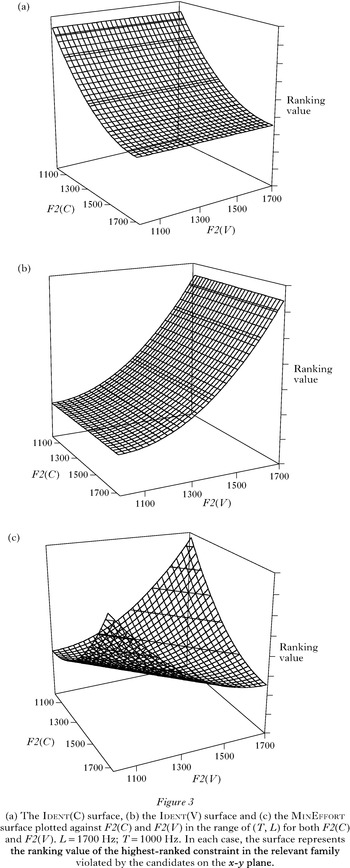
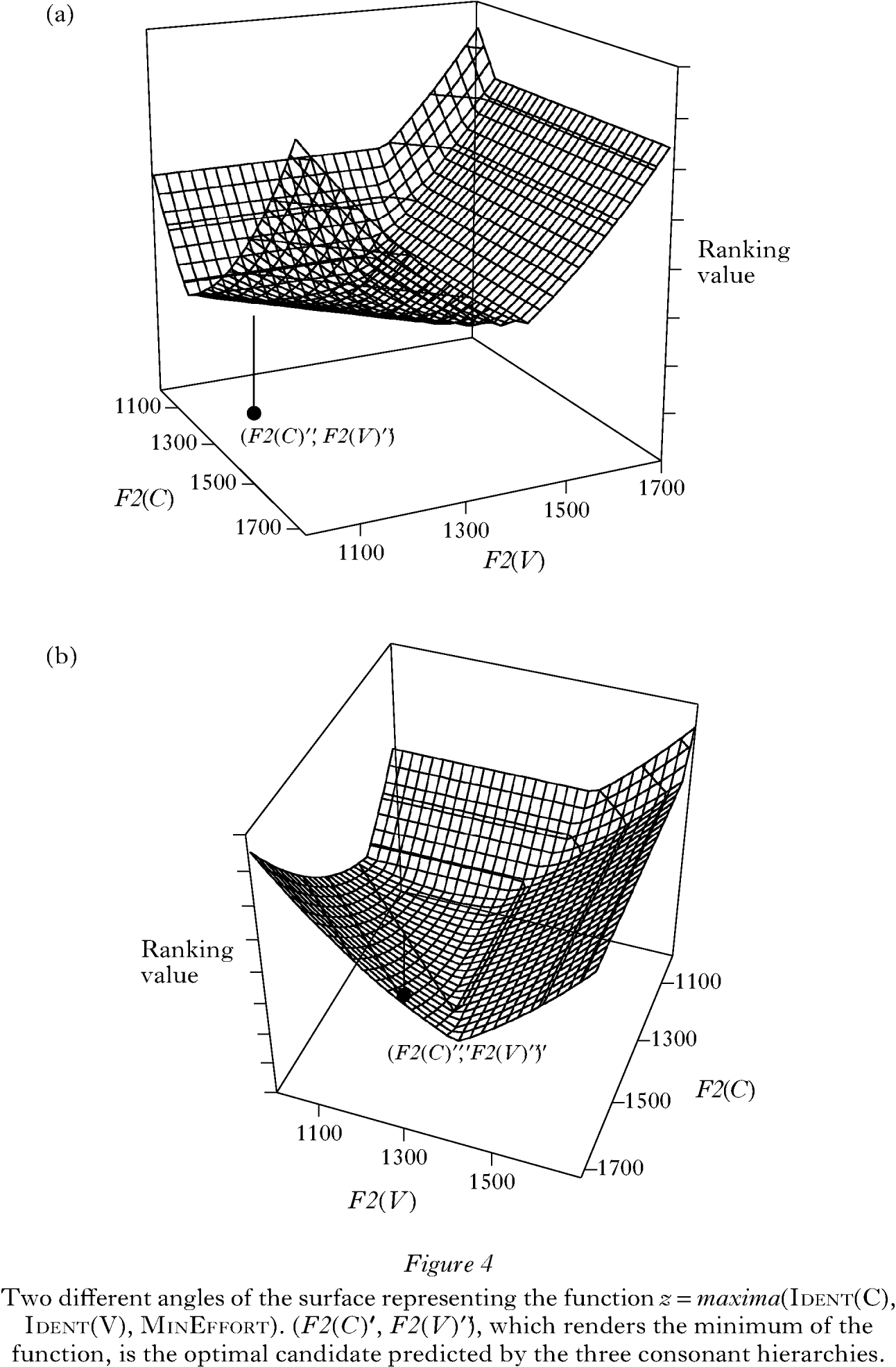
To visualise the interaction among the three constraint families, I first define a three-dimensional space (x, y, z), in which the x and y axes represent F2(C) and F2(V) respectively, and the z axis represents the Ranking Value of constraints that candidates on the x-y plane violate. The Ranking Value of a constraint can be construed as follows: we assume that every constraint is associated with a Ranking Value, and the more highly ranked the constraint is, the greater the Ranking Value of the constraint. Therefore, C1≫C2 is equivalent to RV(C1)>RV(C2), where RV represents Ranking Value.
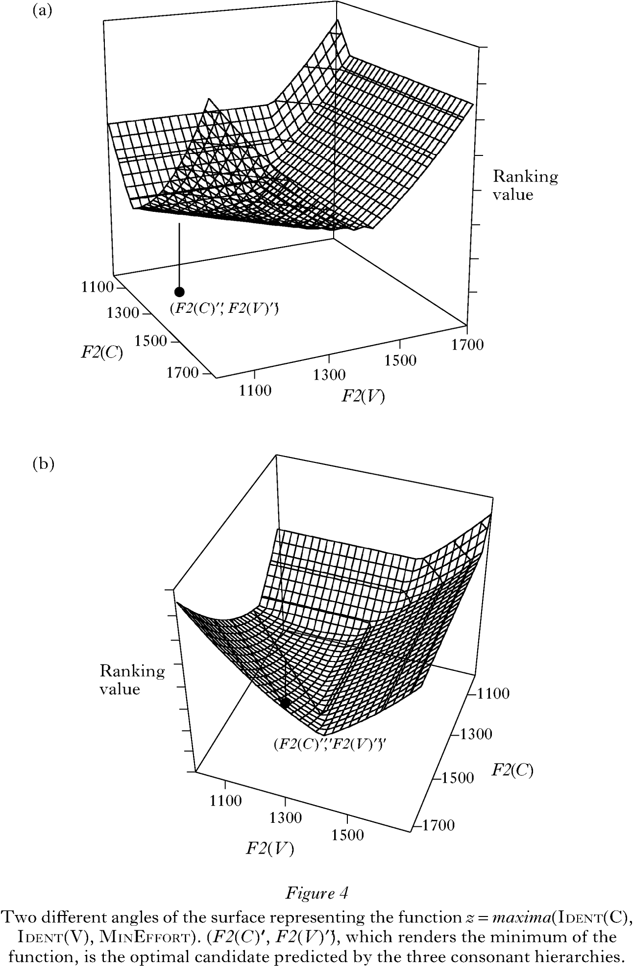
We can represent Ident(C), Ident(V) and MinEffort as three surfaces in this three-dimensional space, as in Fig. 3. The surfaces represent the Ranking Value of the highest-ranked constraint in the family that the candidates on the x-y plane violate, and we only consider the range of F2(C) and F2(V) from T to L, the range within which the winner must fall.Footnote 7 The winner predicted by the constraint hierarchies is the (F2(C), F2(V)) pair that renders the minimum of the function in (19).
(19)

(a) The Ident(C) surface, (b) the iDENT(ff) surface and (c) the mINeFFORT surface plotted against F2(C) and F2(V) in the range of (T, L) for both F2(C) and F2(V). L=1700 Hz; T=1000 Hz. In each case, the surface represents the ranking value of the highest-ranked constraint in the relevant family violated by the candidates on the x-y plane.

This function is plotted from two different angles in Fig. 4. The second surface is derived by rotating the first surface clockwise approximately 60°, looking down on the z axis. The optimal candidate (F2(C)', F2(V)'), which renders the minimum of (19), is indicated in both graphs.
Two different angles of the surface representing the function z=maxima(Ident(C), Ident(ff), MinEffort). (F2(C)', F2(V)'), which renders the minimum of the function, is the optimal candidate predicted by the three consonant hierarchies.
2.1.3 Comparison between constraint weighting and constraint domination
Due to the differences in the nature of constraints, there is in theory one difference in the predictions made by constraint weighting and constraint domination.
Besides the evaluation mode, the faithfulness constraints here also differ from Flemming's model in that they depict a discrete state of affairs: deviations from the input are only penalised when they cross a particular perceptual threshold; otherwise they do not incur faithfulness violations.
A consequence of his difference is that, for constraint weighting, any F2(C)~F2(V) that satisfies T⩽F2(V)⩽F2(C)⩽L can be a possible winner, but for constraint domination, certain F2(C) and F2(V) values will tie as winners and certain other F2(C) and F2(V) values will never win a competition. Let me illustrate this with a hypothetical example. Let us assume that between 1000 Hz and 1700 Hz, only a frequency difference above 20 Hz is perceivable (i.e. 1000 Hz to 1020 Hz is 0 perceptual steps away from 1000 Hz, 1021 Hz to 1040 Hz is 1 perceptual step away from 1000 Hz, etc.), and a frequency difference of 10 Hz is the smallest detectable difference by the articulatory apparatus. If Ident(C)-9, Ident(V)-9 and MinEffort-300 Hz are equally ranked, then the winner can be any F2(C)~F2(V) pair that satisfies the conditions (a) 1500 Hz⩽F2(C)<1520 Hz, (b) 1180 Hz<F2(V)⩽1200 Hz and (c) F2(C)−F2(V)<310 Hz, as all such pairs satisfy Ident(C)-10 and Ident(V)-10, but violate Ident(C)-9 and Ident(V)-9, and also satisfy MinEffort-310 Hz, but violate MinEffort-300 Hz. For example, F2(C)=1500 Hz and F2(V)=1200 Hz, F2(C)=1501 Hz and F2(V)=1194 Hz and F2(C)=1508 Hz and F2(V)=1199 Hz are all possible winners. However, a pair like F2(C)=1505 Hz and F2(V)=1190 Hz will tie with the winners on faithfulness violations, but do worse with MinEffort constraints by violating MinEffort-310 Hz. Therefore, it will never be the winner. This hypothetical example is illustrated in (20).
(20)

I stated that this difference in prediction between constraint domination and constraint weighting is only theoretical because, as a reviewer rightly pointed out, even if the constraint system does not take into account the issue of noticeable differences and generates candidates that the perceptual system cannot differentiate, the differential limens will still play a role in perception, causing the indiscriminable candidates to be learned as one. There may therefore not be an empirical difference between the predictions made by the two approaches.
2.2 Neutralising assimilation
2.2.1 Predictions of the constraint-weighting model
Let us now consider the predictions on /u/~/y/ neutralisation in coronal contexts in Flemming's model, taking into account MinDist and MaxContrasts. Assuming that the MinDist requirement is Δ, and the benefit of keeping the /u/~/y/ constrast is −w n, the overall cost for keeping the contrast is then as in (6) above, and the F2(u) value that renders the smallest overall cost is as in (21).
(21)

Let us remember that this is a simplified model: the Ident(C) constraint, whose cost of violation is w c(F2(t)−L t)2, is only a stand-in for contrast constraints that will yield the F2(t) value when interacting with MinEffort. If we further assume that F2(t) and F2(y) are known, and that Δ is constant, then we can easily adjust the values of we and w v so that any F2(u) value in the range of (0, F2(y)) can render the smallest overall cost; and we can adjust the w n value contributed by MaxContrasts to predict either neutralisation or non-neutralisation, given the F2(u) value. This means that the model is able to predict neutralisation of the /u/~/y/ contrast, but also any /u/~/y/ contrast in which the F2(u) value is in the range of (0, F2(y)).
2.2.2 Predictions of the constraint-domination model
These predictions can be easily made by constraint domination as well. The constraint inventory includes: (a) Ident(C) and MinEffort, which are the same as in (14) and (17), (b) MaxContrasts, which I take as a single constraint that penalises /u/~/y/ neutralisation and (c) MinDist, which I define as a constraint family as in (22a), with the universal ranking in (22b).
(22) MinDistconstraints

For any F2(u) in the range of (0, F2(y)), assuming that F2(y) and F2(u) differ by i perceptual steps, F2(t) and F2(y) are known, and Δf j⩽F2(t)−F2(u)<Δf j+1, the constraint ranking in (23) is sufficient to ensure the preservation of the /u/~/y/ contrast and to give F2(u) as the winner.
(23)

The tableau in (24) illustrates the derivation of a variable F2(u) as the winner. F2(u) violates MinDist-(i+1) as it is only i perceptual steps away from F2(y), and it violates MinEffort-Δf j as the constraint requires the F2 difference between the /t/ and the /u/ to be less than Δf j. But a smaller F2 value that can be controllably implemented (the second candidate) will violate MinEffort-Δf j+1; a greater F2 value that is perceptually closer to F2(y) (the third candidate) will violate MinDist-i; and neutralisation of /u/~/y/ (the last candidate) will violate MaxContrasts, all of which are more highly ranked than the constraints F2(u) violates.
(24)
To predict neutralisation, we only need to ensure that MaxContrasts is ranked lower than either MinDist-(i+1) or MinEffort-Δf j. The intuition is that any F2(u) in the range of (0, F2(y)) may not be a worthwhile contrast with F2(y), because it does not do well enough in either contrast dispersion or effort minimisation.
2.3 Discussion
2.3.1 Factorial typological predictions regarding single outputs
The comparison above between constraint weighting and constraint domination has shown that, in both non-neutralising and neutralising scenarios, they make formally equivalent predictions about the range of possible values as single outputs; their only difference is that the predicted values of constraint weighting are continuous, while those of constraint domination are discrete. This difference stems from the distinct natures of faithfulness constraints in the two approaches: faithfulness violation is calculated in an continuous fashion in constraint weighting, but discretely assessed in the current implementation of constraint domination.
As already mentioned, this difference in prediction may be only theoretical, not empirical, as the differential limens, even if they are not encoded in the grammar, will be relevant to perception and conflate whatever candidates generated by the grammar that cannot be discriminated from each other in the learning process.
2.3.2 The additive effect
Related to the predictions on single outputs is the issue of how the additive trade-off between effort and distinctness constraints can be captured. This trade-off relation is captured intuitively by the summation of violation costs of constraints in the weighting model, and Flemming takes this as an argument for the model. There are two scenarios in which additive effects seem relevant. One is that ‘better vowel distinctiveness together with better consonant distinctiveness can make up for expending more effort’ (Flemming Reference Flemming2001: 33). The other is that when a vowel is flanked between two identical consonants, the consonant effect on the vowel is stronger than when the vowel is only adjacent to one consonant.
But as we have seen in the accounts of both non-neutralising and neutralising assimilation in constraint domination, no reference to constraint conjunction is in fact necessary to capture the first scenario: it is derived from the collective high ranking of Ident(C) and Ident(V) constraints, together with the low ranking of MinEffort. Put differently, given that the effort depends on the realisations of both the consonant and the vowel, the high ranking of Ident(C) or Ident(V) alone plainly does not suffice to justify egregious violations of the MinEffort constraint family. This can be further illustrated by the following examples.
A constraint ranking in which the entire Ident(C) family outranks the MinEffort family, which in turn outranks the entire Ident(V) family, will predict the completely faithful rendition of consonant locus L as F2(C), and an F2(V) identical to F2(C), with no MinEffort violations whatsoever. This is illustrated in the tableau in (25), and it shows that the high ranking of the Ident(C) alone does not justify MinEffort violations (‘(*)’ in the tableau indicates that the constraint may or may not be violated by the candidate).
(25)
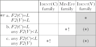
But if the Ident(V) constraint family also outranks the MinEffort family en masse, then the constraint ranking predicts entirely faithful renditions of F2(C) and F2(V) as L and T, as shown in (26). This illustrates that the collective high rankings of Ident(C) and Ident(V) can motivate MinEffort violations. No constraint conjunction is necessary to achieve this effect.
(26)
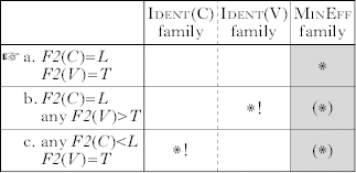
Finally, if the Ident(C), Ident(V) and MinEffort constraint families interleave with each other as in (18), the winner will be an F2(C) which is i perceptual steps away from L and an F2(V) which is j perceptual steps away from T, where F2(C)>F2(V). If we assume L=1700 Hz, T=1000 Hz, F2(C)=1500 Hz and F2(V)=1200 Hz are 9 perceptual steps away from L and T respectively, the tableau in (27) illustrates how F2(C)=1500 Hz, F2(V)=120 Hz can be selected as the winner. In this case, the MinEffort violations incurred by the winner are motivated by the higher ends of both the Ident(C) and Ident(V) families.
(27)

What I have shown above is that the ‘ganging up’ effect of consonant distinctiveness and vowel distinctiveness on effort minimisation does not need constraint conjunction to be modelled in constraint domination. As for the additive effect of having two flanking consonants on either side of the vowel, it can be derived in constraint domination if MinEffort is evaluated on the syllable level rather than only at the juncture of C and V: the effort expenditure for a CVC syllable is greater than that for CV with the same C and V realisations; therefore, a CVC syllable is more stringently evaluated by MinEffort than CV, which would cause a higher likelihood of neutralisation in the former. The minimisation of effort is a general functional principle, and there is thus no a priori reason for its evaluation to be restricted to two adjacent segments and not applicable to other linguistic units, such as the syllable. This essentially replicates this second additive effect in constraint domination, without resorting to constraint conjunction.
It remains an independent question whether additive effects that require constraint conjunction are cross-linguistically attested. Works such as Kirchner (Reference Kirchner1996), Crowhurst & Hewitt (Reference Crowhurst and Hewitt1997), Bonilha (Reference Bonilha2002), Łubowicz (Reference Łubowicz2002), Moreton & Smolensky (Reference Moreton and Smolensky2002) and Tranel & del Gobbo (Reference Tranel, del Gobbo, Wiltshire and Camps2002), among others, argue that they are; but McCarthy (Reference McCarthy, Carpenter, Coetzee and de Lacy2002) and Padgett (Reference Padgett2002) believe that such effects can all be dealt with alternatively. I leave this issue open.
2.3.3 The locus effectFootnote 8
The final significant point of comparison between constraint weighting and constraint domination concerns their factorial typological predictions of the relation among different outputs in the same grammar. For non-neutralising assimilation, constraint weighting predicts a locus effect between F2(C) and F2(V) – the linear relation between the F2 realisation of a consonant and the F2 realisation of different vowels that follow the consonant – as a direct consequence of the quadratic evaluation of constraint penalties; but constraint domination needs very particular rankings of the constraints to predict the linearity between F2(C) and F2(V). Given that the locus effect has been widely reported in the phonetics literature (e.g. Lindblom Reference Lindblom1963, Broad & Clermont Reference Broad and Clermont1987, Klatt Reference Klatt1987, Sussman Reference Sussman1989, Sussman et al. Reference Sussman, McCaffrey and Matthews1991), Flemming takes this an another argument for the constraint-weighting model.
I show in this section that the locus effect can indeed be derived through particular rankings in constraint domination. Furthermore, I show that any function F2(C)=f(F2(V)) predicted by the factorial typology of constraint domination increases monotonically when F2(V) falls between the vowel target T and the consonant target L. This is admittedly a weaker prediction than constraint weighting, but I argue that this weaker prediction might be advantageous when phonetic dimensions other than F2 are considered.
Let us assume that, for a constant consonant target L and various vowel targets T 1, T 2, …, T n, the winning F2(C)~F2(V) realisations are F2(C)1~F2(V)1, F2(C)2~F2(V)2, …, F2(C)n~F2(V)n. To show that the locus effect can be captured, we need to demonstrate that there is a constraint ranking under which the winning F2(C) and F2(V) values are linearly related; in other words, for any i, j between 1 and n, F2(C)j−F2(C)i=k(F2(V)j−F2(V)i), where k is a positive constant.
Let us first take a winning pair F2(C)i~F2(V)i. Clearly, T i⩽F2(V)i⩽F2(C)i⩽L. Let us assume that F2(C)i is C i perceptual steps from L, F2(V)i is V i perceptual steps from T i, and Δf i⩽F2(C)i−F2(V)i<Δf i+1. The constraint ranking that derives the F2(C)i~F2(V)i pair is given in (28), which derives from (18).
(28)
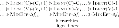
We now need to show that for a different vowel target T j, there is a constraint ranking consistent with (27) that can derive the winning pair F2(C)j~F2(V)j, such that F2(C)j−F2(C)i=k(F2(V)j−F2(V)i).
Let us first assume that T j>T i. I also make the following assumptions about F2(V)j: (a) F2(V)j>F2(V)i, and (b) if F2(V)j is V j perceptual steps away from T j, then V j<V i. These are reasonable assumptions, as a vowel target that is closer to the consonant target (since T j>T i) gives the surface vowel a better chance to be more faithful. From this, we know that Ident(V)-V i≫Ident(V)-V j.
Since F2(C)j=F2(C)i+k(F2(V)j−F2(V)i), and F2(V)j>F2(V)i, k>0, we know that F2(C)j>F2(C)i. Therefore, F2(C)j is perceptually closer to L than F2(C)j. If C j represents the perceptual steps F2(C)j is away from L, then Ident(C)-C i≫Ident(C)-C j.
Phonetic research such as Sussman et al. (Reference Sussman, McCaffrey and Matthews1991) has shown that in the locus equation F2(C)=k∗F2(V)+c, the value of k is less than 1. Since F2(C)j−F2(C)i=k(F2(V)j−F2(V)i), we know that F2(C)j−F2(C)i<F2(V)j−F2(V)i, which means F2(C)j−F2(V)j<F2(C)i−F2(V)i. Therefore, if Δf j⩽F2(C)j−F2(V)j<Δf j+1, then MinEffort-Δf i≫MinEffort-Δf j.
We have thus far shown that (a) Ident(V)-V i≫Ident(V)-V j, (b) Ident(C)-C i≫Ident(C)-C j and (c) MinEffort-Δf i≫MinEffort-Δf j. These rankings determine that it is possible to align the three constraint hierarchies in such a way that Ident(C)-C j, Ident(V)-V j and MinEffort-Δf j are equally ranked, in the meantime leaving the ranking in (28) intact. This is shown in (29), in which the vertical lines indicate the locations of alignment of the three hierarchies. This ranking will not only predict F2(C)i~F2(V)i as the winning pair when the vowel target is T i, but also predict F2(C)j~F2(V)j as the winning pair when the vowel target is T j.
(29)

For T j<T i, with the assumptions that (a) F2(V)j<F2(V)i and (b) F2(V)j is further away from the vowel target than F2(V)i, we can similarly show that (a) Ident(V)-V j≫Ident(V)-V i, (b) Ident(C)-C j≫Ident(C)-C i and (c) MinEffort-Δf j≫MinEffort-Δf i. We can therefore align the rankings of Ident(V)-V j, Ident(V)-C j and MinEffort-Δf j at a location higher than the point of alignment for Ident(V)-V i, Ident(V)-C i and MinEffort-Δf i and this ranking will again predict F2(C)i~F2(V)i and F2(C)j~F2(V)j as the winning pairs for vowel targets T i and T j respectively.
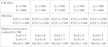
To further illustrate this with a concrete example, let us consider a consonant target L=1700 Hz and vowels targets T=1000 Hz, 1100 Hz, 1200 Hz, 1300 Hz and 1400 Hz. If between 1000 Hz and 1700 Hz, only a frequency difference above 20 Hz is perceivable, then the constraint ranking in (30) will derive the outputs shown in Table I.
(30)

UR~SR pairs predicted by the constraint ranking in (30).

The F2(C)~F2(V) values in Table I indicate that the constraint ranking has succeeded in modelling the following linear relationship: F2(C) = 0⋅25 * F2(V) + 1200 Hz. It is also easy to show that any function F2(C)=f(F2(V)) predicted by the factorial typology of constraint domination increases monotonically when T⩽F2(V)<L. Suppose again that F2(C)i~F2(V)i is the winning output for the input L~T i, which means that Ident(C)-C i, Ident(V)-V i and MinEffort-Δf i are equally ranked. For a different vowel target T j>T i, let us again assume that in the winning pair F2(C)j~F2(V)j, with T j as the vowel target, (a) F2(V)j>F2(V)i and (b) if F2(V)j is V j perceptual steps from T j, then V j<V i. I show here that F2(C)j>F2(C)i.
All candidates with an identical F2 realisation for the vowel – F2(V)j – will tie on the entire Ident(V) hierarchy. Thus the decision will be made by Ident(C) and MinEffort. If F2(C)j<F2(C)i, then the candidate will violate a higher-ranked Ident(C) constraint than the cluster of equally ranked constraints: Ident(C)-C i, Ident(V)-V i and MinEffort-Δf i. But if F2(C)j>F2(C)i, not only will the candidate do better on the Ident(C) hierarchy, but it is also possible to pick an F2(C)j such that F2(C)j−F2(V)j<F2(C)i−F2(V)i. Thus the candidate will only violate constraints that are ranked below the cluster of constraints above.
This reasoning is illustrated in the tableau in (31). F2(C)1, F2(C)2 and F2(C)3 represent F2(C) values that are less than, equal to and greater than F2(C)i respectively. If they are C 1, C 2 and C 3 perceptual steps from L respectively, then clearly C 1>C 2>C 3, which means that F2(C)1 and F2(C)2 both violate higher-ranked Ident(C) constraints than F2(C)3, as Ident(C)-C 1≫Ident(C)-C 2 (same as Ident(C)-C i)≫Ident(C)-C 3. And finally, we can pick an F2(C)3 such that it satisfies the following condition: F2(C)3−F2(V)j<F2(C)i−F2(V)i. Therefore, F2(C)3 only violates a MinEffort constraint lower than MinEffort-Δf i. For clarity, I use real frequency differences such as F2(C)-F2(V)j in lieu of the Δf notation for MinEffort constraints in the tableau.
(31)

We have thus far shown that constraint domination can also model the linear locus effect. One potential drawback of the domination model is that although the monotonicity of the F2(C)~F2(V) relationship is necessarily predicted, the linearity is not. Constraint weighting, in contrast, necessarily predicts the locus effect due to the quadratic evaluation of constraint costs. But on the other hand, F2 is only one of the many dimensions along which the faithfulness and markedness constraints are evaluated. Although the locus effect is widely attested for F2 in the phonetic literature, it is less clear for other formants such as F3. For example, in a study of American English /CVt/ tokens with initial /b d g/ and ten different vowels, Sussman (Reference Sussman1989) showed a linear relationship between the initial consonant and the vowel for F2, but not for F3. Therefore, the necessary prediction of the locus effect for all formants may not be an advantage after all.
3 Conclusion
I have shown in this paper that constraint weighting à laFlemming (Reference Flemming2001) is not a necessary innovation in Optimality Theory. Using constraint families with intrinsic rankings, constraint domination formally predicts the same range of sound realisations as constraint weighting. Moreover, constraint domination can successfully model both the additive effect and the locus effect predicted by constraint weighting.
It must again be acknowledged that the present paper only takes issue with a minor point raised by Flemming (Reference Flemming2001), namely, the mode of constraint evaluation. I do not dispute Flemming's main thesis that both scalar and categorical sound patterns should be accounted for in a unified framework, and the current model accommodates this theoretical standpoint as well. The goal of the paper, therefore, is not to argue for or against phonetics-in-phonology, but to present an alternative model to Flemming's in which this position can be implemented, and to encourage further thinking about the formalisation of phonetic and phonological processes.