





1. Introduction
A large experimental literature documents systematic deviations from Nash equilibrium and even from rationalisable behaviour, and shows that behaviour in strategic settings responds to changes in relative incentives.Footnote 1 This brought to the fore a variety of behavioural models of play in strategic settings, featuring limited reasoning ability (Camerer et al., Reference Camerer, Ho and Chong2004; Nagel, Reference Nagel1995; Stahl & Wilson, Reference Stahl and Wilson1995), payoff-dependent mistakes (McKelvey & Palfrey, Reference McKelvey and Palfrey1995), random beliefs (Friedman & Mezzetti, Reference Friedman and Mezzetti2005; Friedman, Reference Friedman2022), and costly cognition (Alaoui & Penta, Reference Alaoui and Penta2016; Gonçalves, Reference Gonçalves2024). More broadly, these models have been used to explain otherwise-puzzling patterns in settings as diverse as auctions (Bajari & Hortaçsu, Reference Bajari and Hortaçsu2005), financial bubbles (Moinas & Pouget, Reference Moinas and Pouget2013), and responses to monetary policy (Farhi & Werning, Reference Farhi and Werning2019).
Whilst a large literature shows that behaviour in games responds to changes in relative incentives, much less is known about how the level of incentives itself affects strategic behaviour. Strategic settings such as auctions, elections, negotiations, and pricing often differ markedly in the stakes the parties face. Understanding how incentive levels affect strategic behaviour matters for both theory and policy. On the theory side, evidence on how incentive levels affect behaviour can help distinguish whether the key driver is limited reasoning, payoff-dependent mistakes, random beliefs, or costly cognition. On the policy and design side, many interventions work either by changing the strength of incentives or by changing the information available to decision-makers, and the relative effectiveness of these approaches depends on which channel is operative.
Existing evidence on incentive levels in strategic settings is limited, focuses mostly on whether choices change with incentive levels, and is itself hard to interpret.Footnote 2 The evidence is mixed, with choices responding to incentive levels to different extents across strategic environments, which can reflect multiple channels operating at once. Higher incentives make decision mistakes more costly, which can not only reduce mistake-proneness, but may also induce more reasoning and affect the beliefs players form. Moreover, existing designs confound a player’s own-incentive effect with indirect effects operating through higher-order beliefs. This is because a player’s behaviour may react directly to their own incentive level, through reduced payoff-dependent mistakes or greater effort devoted to reasoning, but it may also react indirectly through beliefs about how opponents respond.
This paper experimentally studies how incentive levels affect strategic behaviour. Our design relies on recent advances in experimental methodology to causally identify how own and opponent incentive levels affect actions, beliefs, and response times in strategic settings. Focusing on dominance-solvable games, we show that higher own incentive levels lead to more strategically sophisticated actions (of higher order of rationality), fewer mistakes, and better responses to stated beliefs. Beliefs are also affected: higher incentives lead participants to expect opponents to play more sophisticated actions. Moreover, whereas higher own incentives improve belief accuracy, opponents with higher incentives are harder to predict precisely. Finally, higher incentive levels increase response time, which, in turn, is positively associated with payoffs and both action and belief sophistication.
Three considerations motivate separating own- and opponent-incentive effects. First, different behavioural models make different predictions about which incentive components should matter.Footnote 3 Second, if one varies only overall incentives, then changes in beliefs and higher-order reasoning naturally confound the direct effect of own incentives on behaviour. Finally, since many experimental and applied environments involve asymmetric stakes, understanding separately how behaviour responds to own and opponents’ incentive levels is useful both for interpretation and for design.
To study these issues, we provide an experimental design that separately identifies the effects of own and opponents’ incentive levels on actions, beliefs, and response times. Participants are randomly assigned to treatments that vary own and the opponents’ incentive level and the game played. Our identification strategy relies on a simple opponent-matching protocol adapted from the replacement method (Alaoui & Penta, Reference Alaoui and Penta2016; Alaoui et al., Reference Alaoui, Janezic and Penta2020). This allows us to vary a participant’s own incentive level whilst holding fixed the behaviour relevant for their decision problem, and conversely to vary opponents’ incentive levels whilst holding fixed the participant’s own incentives. The design also fixes higher-order beliefs, in the sense that participants know not only the incentive level faced by their opponent but also the incentive level faced by that opponent’s opponent, and so on. We vary incentive levels by randomly assigning participants to a high- or low-bonus treatment, with choices affecting the probability of receiving the corresponding payment bonus. To focus on initial responses and keep per-decision incentives high-powered, participants complete two unincentivised practice rounds without feedback and then make a single incentivised choice.
We implement this design in two symmetric dominance-solvable normal-form games that differ in strategic complexity. We focus on dominance-solvable games because they provide a clean, theory-grounded ranking of actions and beliefs by strategic sophistication. In the simpler game, the dominance solution is reached after two rounds of maximal iterated elimination of strictly dominated strategies; in the more complex game, it is reached only after three rounds. In both games, level- $k$ actions are identified in a way that is robust to risk attitudes. The games share a number of features with standard environments used to study strategic sophistication — including beauty-contest, undercutting, ring, and related dominance-solvable games (Costa-Gomes & Crawford, Reference Costa-Gomes and Crawford2006; Kneeland, Reference Kneeland2015; Nagel, Reference Nagel1995) — which enables us to relate our results to the existing literature. This makes them especially useful for studying whether incentives affect mistakes, higher-order reasoning, and belief formation in a tightly controlled strategic setting. This results in a 2
 $\times$2
 $\times$2 between-participant design with random assignment, in which over 1600 participants recruited online play only one game and only once.
The paper features four main sets of results. First, higher own incentives make actions more sophisticated, but the relevant margin depends on game complexity. In both games, higher own incentives reduce dominated play and increase play of the level-2 action. The level-2 action corresponds to the dominance-solution action in the simpler game. In the more complex game, the level-3 action is the dominance-solution action, but its frequency does not change with higher incentives. Opponents’ incentive levels have qualitatively similar but substantially weaker effects.
Second, the data support a payoff-sensitivity channel consistent with a subjective version of quantal response. Actions with higher subjective expected payoff (as per stated beliefs) are chosen more often, but this payoff-rank monotonicity does not carry over to objective expected payoffs (as given by empirical frequency of opponents’ actions). Higher own incentives not only substantially increase best-response rates to stated beliefs but also shift choices toward better responses to participants’ reported beliefs. A subjective logit quantal-response specification fits the data much better than an analogous specification based on empirical opponent frequencies, underscoring the importance of elicited beliefs for understanding observed choices.
Third, incentives affect beliefs in a way that mirrors actions. Higher own incentives reduce the probability assigned to dominated play and shift beliefs toward more sophisticated opponent behaviour. In the 2-Step game, this shift extends to the dominance-solution action. In the 3-Step game, however, beliefs move primarily toward intermediate level-1 and level-2 actions rather than toward the level-3 dominance solution. The effects of opponent incentive level are qualitatively similar, but sharply muted. Higher own incentives also improve several dimensions of belief accuracy, whereas opponents facing higher incentives become harder to predict precisely.
Fourth, response times provide suggestive evidence on mechanism. Higher own incentives increase response times by over 40% in both games. Additionally, controlling for incentives and individual characteristics as well as longer response times are associated with better performance: higher best-response rates, higher expected payoffs, fewer dominated choices, and more sophisticated beliefs. Finally, we explore how response times relate to both actions and beliefs and find that deliberating for longer is associated with more sophisticated actions being chosen and with more sophisticated beliefs being reported. Specifically, in both games, the frequency of dominated actions monotonically decreases with time, the level-1 action is the modal action at short response times and its frequency decreases with deliberation, whilst the level-2 action frequency increases. Beliefs track these patterns consistently: longer response times are also associated with greater belief mass on both the level-1 and level-2 actions. Interestingly, the frequency of and the belief about the dominance-solution action in the more complex game, the level-3 action, are fairly invariant over time. Noting that response time is an informative, even if imperfect, proxy for cognitive effort (Caplin et al., Reference Caplin, Csaba, Leahy and Nov2020; Gill & Prowse, Reference Gill and Prowse2022), we interpret these patterns as suggestive evidence that higher incentives affect behaviour through both reduced payoff-dependent mistakes and greater effort devoted to reasoning.
Our robustness analysis shows that the main patterns are stable within our setup. The results replicate across participant pools, remain qualitatively similar under alternative specifications, and are not driven by participants with weaker attention or poorer comprehension. We also discuss the extent to which alternative explanations based on other-regarding preferences may still matter, whilst showing that the treatment effects in the data are difficult to reconcile with such channels.
These findings should nevertheless be interpreted within the scope of a tightly controlled benchmark environment, precisely one in which direct confounds from feedback, learning, and payoff externalities are reduced. We therefore do not claim to speak to all strategic environments. More generally, it is well known that very high or unfamiliar incentive levels can sometimes backfire, so our conclusions should not be extrapolated mechanically to settings with extreme stakes or to environments in which additional motivational channels are likely to be important (Ariely et al., Reference Ariely, Gneezy, Loewenstein and Mazar2009; Camerer & Hogarth, Reference Camerer and Hogarth1999; Enke et al., Reference Enke, Gneezy, Hall, Martin, Nelidov, Offerman and van de Ven2023).
Within those limits, this paper contributes well-identified evidence on how incentive levels affect reasoning, mistakes, beliefs, and response times in a strategic setting. By separately identifying own- and opponent-incentive effects, the paper clarifies through which channels higher incentives change behaviour and how those effects depend on strategic complexity. Taken together, our results suggest that, at familiar incentive levels, higher incentives increase action sophistication both by reducing the propensity to make mistakes and by increasing the incentive to reason further and form better beliefs. At the same time, the fact that action sophistication and belief accuracy increase in the simpler game, but less so or not at all in the more complex game, implies that one should not expect changes in incentives to have uniform effects across strategic environments that differ in complexity. Our findings therefore caution both against inferring universally low levels of sophistication from evidence obtained under low-powered incentives and against relying on predictions that require high levels of sophistication in complex but low-stakes environments.
The remainder of the paper proceeds as follows. Section 2 presents the hypotheses, experimental design, and identification strategy. Sections 3, 4, 5, and 6 report the results on actions, payoff-dependent mistakes, beliefs, and response times. Section 7 discusses alternative explanations, robustness checks, and limitations. Section 8 concludes.
1.1. Related literature
This paper contributes to four related strands of literature.
Strategic sophistication and bounded rationality. A large literature documents persistent deviations from Nash equilibrium and substantial heterogeneity in strategic sophistication. This is true in dominance-solvable environments such as beauty-contest, undercutting, and ring games (Costa-Gomes & Crawford, Reference Costa-Gomes and Crawford2006; Kneeland, Reference Kneeland2015; Nagel, Reference Nagel1995), as well as in many other normal-form games (Arad & Rubinstein, Reference Arad and Rubinstein2012; Fudenberg & Liang, Reference Fudenberg and Liang2019). Experimental work also shows that action sophistication is not stable across games and depends importantly on what players believe about their opponents (Agranov et al., Reference Agranov, Potamites, Schotter and Tergiman2012; Georganas et al., Reference Georganas, Healy and Weber2015). These findings motivated several models of bounded rationality in games, the common theme of which is that observed play reflects a combination of shallow reasoning, payoff-dependent mistakes, and costly cognition.Footnote 4 This paper studies the effect of incentive levels on choices, beliefs, and response times in an environment where actions and beliefs admit a clear ranking by strategic sophistication. The design allows us to distinguish shifts away from dominated play from shifts toward intermediate and dominance-solution actions, and to separate changes in mistake propensity from changes in the depth of reasoning.
Incentives and mistakes in strategic settings: A substantial literature studies how behaviour reacts to changes in relative incentives across actions. This includes work on matching-pennies games (Ochs, Reference Ochs1995; McKelvey et al., Reference McKelvey, Palfrey and Weber2000), traveler’s dilemma (Capra et al., Reference Capra, Goeree, Gomez and Holt1999), joker games (Melo et al., Reference Melo, Pogorelskiy and Shum2019), and the modified 11–20 game (Alaoui & Penta, Reference Alaoui and Penta2016; Alaoui et al., Reference Alaoui, Janezic and Penta2020). Closest to our paper is Alaoui et al. (Reference Alaoui, Janezic and Penta2020). They show that changing relative incentives in a replacement design shifts behaviour toward lower numbers and emphasise the role of beliefs about opponents’ sophistication. The broad lesson from this literature is that players react strongly when one action becomes more attractive than another, and that beliefs about opponents often play a central role in mediating these responses.
Our paper differs in two key respects. First, we study absolute incentive levels whilst holding relative incentives between actions fixed. Second, we separately identify own- and opponent-incentive effects on both choices and beliefs. Our findings consistently highlight the central role of beliefs. We also show that, even holding relative incentives fixed, higher own incentives operate through reduced payoff-dependent mistakes and greater effort devoted to reasoning.
The literature on absolute incentive levels in strategic settings is much thinner. Existing evidence shows that higher stakes sometimes can move behaviour toward equilibrium benchmarks, for instance in centipede games (McKelvey & Palfrey, Reference McKelvey and Palfrey1992; Rapoport et al., Reference Rapoport, Stein, Parco and Nicholas2003). The broader methodological literature has long stressed that stake variation is useful both for assessing robustness and for understanding the trade-off between incentives and decision costs (Camerer & Hogarth, Reference Camerer and Hogarth1999; Smith & Walker, Reference Smith and Walker1993). Our contribution is to provide evidence on absolute incentives in a strategic setting whilst jointly observing choices, elicited beliefs, and response times.
Our results also speak to the literature on stochastic choice in games. Beginning with quantal response equilibrium, a large body of work models strategic behaviour as probabilistic choice — as in discrete choice (Luce, Reference Luce1959; McFadden, Reference McFadden and Karembka1974) and costly control models (Fudenberg et al. Reference Fudenberg, Iijima and Strzalecki2015) — in which better actions are chosen more often, but not always (Goeree et al., Reference Goeree, Holt and Palfrey2005; Mattsson & Weibull, Reference Mattsson and Weibull2002; McKelvey & Palfrey, Reference McKelvey and Palfrey1995). In this class of models, higher incentives should, under suitable conditions, sharpen the relation between expected payoffs and choice probabilities. We provide evidence in line with this logic, but with an important qualification: monotonicity and best-response improvements are much clearer when expected payoffs are computed using participants’ stated beliefs than when they are computed using empirical opponent frequencies. This places beliefs at the centre of any explanation based on payoff-dependent mistakes.
Beliefs in strategic settings: Our paper also contributes to the literature that elicits beliefs in games and studies how they vary systematically with the strategic environment. A large empirical literature shows that stated beliefs are informative about behaviour, though far from perfectly aligned with observed choices (Costa-Gomes & Weizsäcker, Reference Costa-Gomes and Weizsäcker2008; Nyarko & Schotter, Reference Nyarko and Schotter2002; Rey-Biel, Reference Rey-Biel2009). Related work shows that eliciting beliefs can itself affect play, including in dominance-solvable environments (Croson, Reference Croson1999, Reference Croson2000; Gächter & Renner, Reference Gächter and Renner2010), and that beliefs respond systematically to features of the game (Agranov et al., Reference Agranov, Potamites, Schotter and Tergiman2012; Friedman & Ward, Reference Friedman and Ward2022).
Our paper contributes to this literature in two ways. First, we examine directly how own and opponents’ incentive levels affect the beliefs participants form about others’ actions. Second, we relate elicited beliefs to observed choices and show that subjective expected payoffs explain behaviour much better than expected payoffs computed from empirical opponent frequencies. In this sense, the paper supports the view that beliefs are informative about strategic behaviour, but also that understanding how incentives affect beliefs is essential for interpreting observed play.
Response times in strategic settings: Finally, our paper relates to the literature using response times to study strategic behaviour. Response times have been used to classify participants, to predict choices and sophistication, and as an informative proxy for cognitive effort (Frydman & Nunnari, Reference Frydman and Nunnari2023; Gill & Prowse, Reference Gill and Prowse2022; Proto et al., Reference Proto, Rustichini and Sofianos2019; Rubinstein, Reference Rubinstein2007, Reference Rubinstein2016; Schotter & Trevino, Reference Schotter and Trevino2021).Footnote 5 Particularly relevant is Alós-Ferrer and Buckenmaier (Reference Alós-Ferrer and Buckenmaier2021), who study response times in beauty-contest and 11–20-type games.
We differ by providing a design that separately identifies how own and opponents’ incentive levels affect response times, and by relating response times jointly to actions, elicited beliefs, and payoff performance. More broadly, our paper connects the strategic response-time literature to the growing evidence on incentives and effort in non-strategic tasks (Ariely et al., Reference Ariely, Gneezy, Loewenstein and Mazar2009; Caplin et al., Reference Caplin, Csaba, Leahy and Nov2020; Dean & Neligh, Reference Dean and Neligh2023; Enke et al., Reference Enke, Gneezy, Hall, Martin, Nelidov, Offerman and van de Ven2023). Our findings show that higher incentives increase response times, but performance gains are limited by the complexity of the strategic environment.
In short, these connections place the paper at the intersection of the literatures on strategic sophistication, incentives in games, belief formation, and costly reasoning.
2. Hypotheses and experimental design
2.1. Hypotheses
In this section, we present our hypotheses. Throughout, we consider finite normal-form games,  $\Gamma=\langle I, A, u \rangle$, where
 $I$ denotes the set of players,
 $A_i$ the action set of player
 $i$,
 $A_{-i}$ the action profiles of player
 $i$’s opponents,
 $A:=\times_i A_i$ the set of action profiles, and
 $u_i:A\to \mathbb R$ player
 $i$’s payoff function, with
 $u:={u_i}_{i\in I}$. As is conventional, we extend payoffs to the space of probabilities over actions, and write
 $-i$ to denote player
 $i$’s opponents.
Our main interest is in how incentive levels affect strategic behaviour. For any two games  $\Gamma$ and
 $\tilde\Gamma$ that are identical in all except that player
 $i$’s payoffs are scaled up — so that
 $\tilde u_i=\lambda u_i$ for some
 $\lambda \gt 1$ — we say that player
 $i$ has a higher incentive level in
 $\tilde\Gamma$ than in
 $\Gamma$.
Our first hypothesis relates to the effect of incentives on action sophistication. We use rationalisability to formalise this concept. An action is  $k$-rationalisable if it is a best response to some distribution over opponents’
 $(k-1)$-rationalisable actions, and it is rationalisable if it is
 $k$-rationalisable for all
 $k$.Footnote 6 We say that action
 $a_i$ is more sophisticated than action
 $a_i'$ if (i) there exists some
 $k$ such that
 $a_i$ is
 $k$-rationalisable whereas
 $a_i'$ is not, or (ii) if these are both
 $k$-rationalisable but
 $a_i$ iteratively strictly dominates
 $a_i'$.
Although experiments routinely find positive choice frequencies for non-rationalisable actions (e.g.Costa-Gomes & Weizsäcker, Reference Costa-Gomes and Weizsäcker2008; Rey-Biel, Reference Rey-Biel2009), it remains unclear whether and how incentive levels affect the sophistication of play. Differently from payoff distortions, increasing incentive levels leaves relative incentives unchanged and thus the sets of  $k$-rationalisable action distributions unaffected. Existing models also yield different predictions. Many prominent models predict there to be no changes in behaviour in response to incentive levels. This is true of Nash equilibrium (Nash, Reference Nash1951), level-
 $k$ (Nagel, Reference Nagel1995; Stahl & Wilson, Reference Stahl and Wilson1994, Reference Stahl and Wilson1995), cognitive hierarchy (Camerer et al., Reference Camerer, Ho and Chong2004), regret minimisation (Bell, Reference Bell1982; Loomes & Sugden, Reference Loomes and Sugden1982), uncertainty-aversion equilibrium (Bade, Reference Bade2011; Klibanoff, Reference Klibanoff1996), random and noisy-belief equilibria (Friedman & Mezzetti, Reference Friedman and Mezzetti2005; Friedman, Reference Friedman2022), and sampling equilibrium (Osborne & Rubinstein, Reference Osborne and Rubinstein1998, Reference Osborne and Rubinstein2003), among others. In other models, as endogenous depth of reasoning in symmetric games (Alaoui & Penta, Reference Alaoui and Penta2016), increasing a player’s incentive level may affect that player’s actions but not others’.Footnote 7 And other models still make no clear prediction on how action sophistication is affected by incentive levels, as is the case of regular quantal response equilibrium (Goeree et al., Reference Goeree, Holt and Palfrey2005).
Intuition would suggest that by increasing a player’s incentive level, not only that player’s action sophistication increases, but also that opponents can, to some extent, anticipate this and adjust their behaviour accordingly. We formulate this as our first hypothesis:
Hypothesis 1. (Action Sophistication)
Action sophistication increases in (a) own incentive level and (b) opponents’ incentive level.
Although testing Hypothesis 1 is in itself a contribution of this paper, we seek to shed light on mechanisms, that is, why incentive levels may affect choices.
One possible channel is that higher incentives make mistakes more costly, reducing the frequency of suboptimal choices. This is the logic underlying structural quantal response models, in which the probability of choosing an action depends on the vector of expected payoffs. Both models of stochastic choice based on random utility with additive i.i.d. payoff disturbances (McFadden, Reference McFadden and Karembka1974; McKelvey & Palfrey, Reference McKelvey and Palfrey1995) and those based on additive perturbed utility or costly precision (Fudenberg et al., Reference Fudenberg, Iijima and Strzalecki2015; Mattsson & Weibull, Reference Mattsson and Weibull2002) predict, under mild conditions, that higher incentives lead better actions being chosen more often (see Appendix C.1). More generally, regular quantal response equilibrium requires actions with higher expected payoffs to be chosen more frequently (Goeree et al., Reference Goeree, Holt and Palfrey2005). To assess support for this class of models, we test the following hypothesis:
Hypothesis 2. (Quantal Responding)
(a) Best-response rates increase in own incentive level. (b) Actions with higher expected payoff are chosen more often.
Another possible channel through which incentives may affect choices is by affecting players’ beliefs. Previous work shows that beliefs about opponents’ sophistication can help explain the choice of non-rationalisable actions. For example, sophistication of play changes depending on whether players are informed about opponents’ characteristics associated with sophistication, such as chess ratings (Palacios-Huerta & Volij, Reference Palacios-Huerta and Volij2009) or their educational background (Agranov et al., Reference Agranov, Potamites, Schotter and Tergiman2012; Alaoui et al., Reference Alaoui, Janezic and Penta2020). In our setting, higher incentives may induce greater effort in understanding the game, leading participants to think more carefully about opponents’ payoffs and to assign lower probability to opponents choosing non-rationalisable actions.
The effect of incentive level on beliefs about the opponent may depend on both own and opponent incentive levels. On the one hand, if higher incentives induce more sophisticated play, then participants should expect more sophisticated behaviour from opponents facing higher incentives. On the other hand, if reasoning about the game is costly, then higher own incentives raise the value of forming more accurate beliefs. This motivates our next hypothesis:
Hypothesis 3. (Belief Sophistication)
Beliefs about opponents’ strategic sophistication increase with (a) own incentive level and (b) opponents’ incentive level. Furthermore, (c) belief accuracy increases with own incentive level.
Finally, we consider whether higher incentives induce greater cognitive effort and whether such effort is associated with better decisions. In line with recent models of sequential reasoning in games (Alaoui & Penta, Reference Alaoui and Penta2016, Reference Alaoui and Penta2022; Gonçalves, Reference Gonçalves2024), we conjecture that increasing a player’s incentive level induces greater cognitive effort and, in turn, results in better choices. Whilst greater effort need not always translate into longer deliberation, as it may instead take the form of more focused thinking, we follow existing literature in taking response time as an informative proxy for cognitive effort — see Gill and Prowse (Reference Gill and Prowse2022) and references therein. Our final hypothesis is:
Hypothesis 4. (Response Time)
(a) Response time increases in one’s own incentive level and (b) expected payoff increases with response time.
2.2. Experimental design and identification strategy
Identification strategy: Identifying the effect of incentives on behaviour in strategic settings poses a fundamental challenge. A higher incentive level for player  $i$ may have a first-order, direct effect on the player’s behaviour by motivating them to choose better actions, make fewer mistakes, or forming better beliefs. But it may also generate indirect effects through higher-order reasoning: player
 $i$ may expect opponents to respond to
 $i$’s higher incentives, and may adjust behaviour accordingly. To study the effect of incentive levels on strategic behaviour, it is then important to separate first-order, direct effects from higher-order, indirect effects, operating through beliefs about others’ responses.
Our identification strategy relies on a simple opponent-matching protocol, summarised in Figure 1. Participants are assigned both a role in the game and an incentive group, where the group determines their own incentive level and the incentive level of the opponent whose behaviour is relevant for their decision problem. First, we have two incentive groups — (High, High) and (Low, Low) in Figure 1 — in which all players face the same incentive level and know their opponents do as well. Second, we have another two incentive groups — (High, Low) and (Low, High) in Figure 1 — in which participants are matched with opponents with a different incentive level. The opponents themselves are randomly drawn from the other two groups, so that participants in (High, Low) are matched with opponents from (Low, Low), and participants in (Low, High) are matched with opponents from (High, High). This design allows us (i) to hold fixed the opponent’s behaviour whilst varying own incentives, thereby identifying the effect of own incentives on choices and beliefs; and (ii) to hold fixed own incentives whilst varying opponents’ incentives, thereby identifying how beliefs and behaviour respond to the incentive level faced by opponents. Importantly, this procedure also fixes higher-order incentives: it determines not only the incentive level faced by a participant’s opponent, but also the incentive level faced by that opponent’s opponent, and so on.Footnote 8
Opponent matching procedure

This approach corresponds to a version of the replacement method featured in Alaoui and Penta (Reference Alaoui and Penta2016) and Alaoui et al. (Reference Alaoui, Janezic and Penta2020), and is also related to observer-based designs such as Huck and Weizsäcker (Reference Huck and Weizsäcker2002). A key feature of the design is that, for participants in the mixed-incentive groups (High, Low) and (Low, High), the action they choose does not enter the payoff determination of the opponent whose behaviour is payoff-relevant for them. To avoid making this feature unique to those groups, our implemented matching protocol is so that the same property holds throughout the design: the participant whose action is payoff-relevant for player  $i$ is never someone whose own payoff is determined by
 $i$’s action.Footnote 9
Given this matching procedure and random assignment across incentive groups, identification of causal effects of incentive levels is obtained by comparing outcomes — choices, beliefs, and response times — across participants who differ in own incentives or in opponents’ incentives.
Games: Participants faced one of the two normal-form games shown in Figure 2. Both are dominance-solvable and have similar payoff structures. The game in panel (a) requires two rounds of (maximal and simultaneous) iterated elimination of strictly dominated strategies to reach the dominance-solution action, whereas the game in panel (b) requires three rounds.
Games (a) 2-Step game (b) 3-Step game

Fig 2 Long description
The table has two side-by-side payoff matrices. Payoff values are shown as ordered pairs, with no units shown. Each matrix has 4 rows for Player 1 actions and 4 columns for Player 2 actions. The image A showing a table with columns: Actions, Player 2 a1, Player 2 a2, Player 2 a3, Player 2 a4. Rows: Player 1 a1, Player 1 a2, Player 1 a3, Player 1 a4. Diagonal cells where Player 1 action equals Player 2 action are 40, 40 in all four diagonal positions. Row 1 values for Player 1 a1 across Player 2 a1 to a4 are 40, 40; 70, 30; 80, 20; 10, 10. Row 2 values for Player 1 a2 are 30, 70; 40, 40; 70, 30; 80, 20. Row 3 values for Player 1 a3 are 20, 80; 30, 70; 40, 40; 70, 30. Row 4 values for Player 1 a4 are 10, 10; 20, 80; 30, 70; 40, 40. The image B showing a table with columns: Actions, Player 2 a1, Player 2 a2, Player 2 a3, Player 2 a4. Rows: Player 1 a1, Player 1 a2, Player 1 a3, Player 1 a4. Diagonal cells where Player 1 action equals Player 2 action are 40, 40 in all four diagonal positions. Row 1 values for Player 1 a1 across Player 2 a1 to a4 are 40, 40; 70, 30; 10, 20; 10, 10. Row 2 values for Player 1 a2 are 30, 70; 40, 40; 70, 30; 10, 20. Row 3 values for Player 1 a3 are 20, 10; 30, 70; 40, 40; 70, 30. Row 4 values for Player 1 a4 are 10, 10; 20, 10; 30, 70; 40, 40. Differences visible between the two matrices include these cells: Player 1 a1 with Player 2 a3 is 80, 20 in the left matrix and 10, 20 in the right matrix; Player 1 a2 with Player 2 a4 is 80, 20 in the left matrix and 10, 20 in the right matrix; Player 1 a3 with Player 2 a1 is 20, 80 in the left matrix and 20, 10 in the right matrix; Player 1 a4 with Player 2 a2 is 20, 80 in the left matrix and 20, 10 in the right matrix.
The games have the useful property that actions can be ranked naturally by strategic sophistication. First, if  $a_{n+1}$ is
 $k$-rationalisable, then so is
 $a_n$. Second, if both
 $a_{n}$ and
 $a_{n+1}$ are
 $k$- but not
 $(k+1)$-rationalisable, then
 $a_n$ (iteratedly) strictly dominates
 $a_{n+1}$.Footnote 10 Accordingly, we will throughout treat
 $a_n$ as more strategically sophisticated than
 $a_{n+1}$. We note that, assuming a level-0 player uniformly randomises, level-
 $k$ actions are also uniquely pinned down in a way that does not depend on participants’ risk attitudes. In the 2-Step game,
 $a_2$ corresponds to the level-1 action regardless of risk preferences, and
 $a_1$ to the level-2 action; both
 $a_3$ and
 $a_4$ are strictly dominated. In the 3-Step game, the level-1, -2, and -3 actions are, respectively,
 $a_3$,
 $a_2$, and
 $a_1$.
The preceding discussion shows why these games are useful for our purposes. Because they admit a clean, theory-grounded ranking of actions and beliefs by strategic sophistication, they allow us to study whether incentives affect mistakes, higher-order reasoning, and belief formation in a tightly controlled environment. In addition, we specifically chose four-action games because this is the smallest action space that allows us to vary the number of elimination rounds with only minor payoff changes, and we imposed symmetry to improve statistical power and reduce data requirements. The games are related to 11–20 (Arad & Rubinstein, Reference Arad and Rubinstein2012) and other undercutting games (Costa-Gomes & Crawford, Reference Costa-Gomes and Crawford2006; Georganas et al., Reference Georganas, Healy and Weber2015; Nagel, Reference Nagel1995) in that they induce ordered steps of strategic reasoning, but differ in that our games are dominance-solvable and admit a clean ranking of actions by strategic sophistication.
Other design details and logistics: The experiment implemented a  $2\times2\times2$ design, corresponding to own incentive level, opponents’ incentive level, and the game played (2-Step or 3-Step game). Participants were assigned uniformly at random to one of the eight treatments and played only once.
The experiment used binary-lottery incentives and game payoffs corresponded to the probability of receiving a prize of  $x$ rather than $2.00. We presented exactly the same game representation across incentive conditions. This allows us to isolate the effect of incentives whilst holding the strategic structure fixed and avoids potential confounds arising from presenting different payoff numbers due to perceptual or salience effects. In the high-incentive treatment,
 $x$=$22.00; in the low-incentive treatment,
 $x$=$2.50. We chose the high incentive level to maximise treatment variation; the low incentive level nevertheless exceeds the expected payment per game in several related experiments.Footnote 11
The experimental design induces incentive-compatible elicitation of both actions and beliefs under weak assumptions. To this end, we (i) restricted the experiment to a single paid round, thereby also ruling out non-feedback learning (Weber, Reference Weber2003), and (ii) paid either the action task or the belief task, but not both, to avoid hedging concerns (Blanco et al., Reference Blanco, Engelmann, Koch and Normann2010). Actions selected determine game payoffs, which correspond to a probability of getting the prize. The order of rows and columns was randomised and participants were informed of this. Beliefs  $b_i=(b_{i,1},b_{i,2},b_{i,3},b_{i,4}) \in \Delta(A_i)$, interpreted as reported probabilities that the opponent chooses each action, were incentivised using a binarised scoring rule (Hossain & Okui, Reference Hossain and Okui2013). Choices and beliefs were elicited simultaneously to reduce the mismatch between choices and beliefs as suggested by existing evidence (see
Costa-Gomes & Weizsäcker, Reference Costa-Gomes and Weizsäcker2008, Figure 4), and one of them was randomly selected for payment. In the instructions, we also explicitly explained that the payment rule was designed to reward choosing the action that maximises expected points given one’s beliefs, as well as to report beliefs truthfully.
We took several steps to reduce the scope for focal-point effects and other-regarding motives to mechanically account for the observed treatment differences. First, we chose games in which the dominance-solution outcome is neither Pareto dominant nor Pareto dominated, as is true for most outcomes in the games. Second, for most outcomes, the same payoff pair is associated with multiple action profiles. Third, because higher incentives can increase coordination on focal points (Parravano & Poulsen, Reference Parravano and Poulsen2015), we randomly shuffled the order of rows and columns, reducing the salience of visually symmetric payoff configurations and action labels. And fourth, the matching protocol was random and asymmetric, and this was explicitly explained to participants. We return to these concerns in Section 7.1, where we discuss the extent to which the treatment effects are consistent with alternative explanations based on other-regarding preferences.
The experiment proceeded as follows: (i) participants received instructions and completed comprehension and attention checks; (ii) participants played two unincentivised practice rounds without feedback;Footnote 12 (iii) own and opponent incentive levels were revealed;Footnote 13 (iv) actions and beliefs were elicited simultaneously; and (v) participants completed a short socio-demographic survey. Instructions and interface screenshots are provided in Online Appendix A.
We recruited 834 participants on Amazon Mechanical Turk (MTurk) in 8-10 and 15 January 2020 and, for replication and robustness purposes, 880 participants on Prolific in 22-23 January 2026, ensuring 100 participants in each treatment. This additional sample also allows us to assess whether the main treatment patterns are robust to a less salient emphasis on incentives.Footnote 14 In both samples, participants were adults residents in the United States of America with approval rates of at least 95%. We find only minor differences across platforms and therefore report results for the pooled sample; we expand on this in Section 7.2. Participants faced no time limit. Average duration and hourly earnings were approximately 22 minutes and $24.97 on MTurk, and 17 minutes and $23.43 on Prolific. We also collected socio-demographic information, including age and education; see Appendix A.6 for details.
3. Incentives and action sophistication
We first examine whether and how incentive levels affect action sophistication (Hypothesis 1).
Our first observation is that participants do not always play the dominance-solution action,  $a_1$. Table 1 shows substantial heterogeneity in action frequencies across the eight treatments. Dominance play ranges from 13.7% to 56.6%, whilst dominated play — corresponding to actions
 $a_3$ and
 $a_4$ in the 2-Step game and action
 $a_4$ in the 3-Step game — ranges from 5.9% to 28.4%. The raw frequencies already suggest that own incentives matter more in the 2-Step game, whereas in the 3-Step game dominance play remains low across all treatments.
Action frequency, average beliefs distributions, and response time

Notes: This table reports treatment-level summary statistics. Each participant is assigned to one treatment, defined by the game (2-Step or 3-Step game), own incentive level (high or low), and opponents’ incentive level (high or low). Columns (4)–(7) report action frequencies, columns (8)–(11) report mean belief distributions, and column (12) reports mean response time in seconds. Participants play one game and make one incentivised decision.
We next test whether incentive levels affect the frequency of dominance and dominated play. We consider the following specification:
 \begin{equation}
y_i=\beta_0+\beta_1 H_i +\beta_2 H_{-i}+\text{Controls}_i+\epsilon_i,
\end{equation}
where  $H_i$ is an indicator variable equal to 1 if participant
 $i$ faces a high own incentive level, and
 $H_{-i}$ is an analogous indicator equal to 1 if participant
 $i$’s opponent faces a high incentive level. Controls refer to participants’ socio-demographic characteristics.Footnote 15 When testing for the effect of incentive levels on dominance play, the dependent variable
 $y_i$ is an indicator equal to 1 if participant
 $i$ chose the dominance-solution action and 0 otherwise. When testing the effect of incentives on dominated play, we use the analogous indicator for whether the participant chose a strictly dominated action. Table 2 summarises the results.
Incentive level, dominance, and dominated play (Hypothesis 1)

Table 2 Long description
Regression results link incentive levels to whether participants chose the dominance-solution action or a strictly dominated action, reported separately for 2-step and 3-step games. In the 2-step game, high own incentives are associated with a large increase in dominance play (about 19.48, statistically significant) and a large decrease in dominated play (about minus 12.86, statistically significant). In the 3-step game, high own incentives are near zero for dominance play (about minus 1.01, not statistically significant) but still reduce dominated play (about minus 5.27, statistically significant). High opponent incentives show a small positive association with dominance play in the 2-step game (about 5.95, marginally significant) and are close to zero in the 3-step game (about 1.75, not statistically significant). Opponent incentives are not meaningfully related to dominated play in either game (about minus 0.71 and 0.37, both not statistically significant). All models include participant controls; model fit is low (R squared about 0.02 to 0.06) with sample sizes of 837 for 2-step and 877 for 3-step. Standard errors are robust, so statistical significance should be interpreted with that uncertainty measure in mind.
Notes: This table reports estimates from the regression specified in equation (1), where the dependent variable is an indicator for whether the participant chose the dominance-solution action (columns (1) and (2)) or a strictly dominated action (columns (3) and (4)). High Own/Opponent Incentives are indicators for whether the participant and their opponent face a high incentive level. 2 Steps and 3 Steps denote the two games in the experiment; see Figure 2. Controls refer to participants’ socio-demographic characteristics. Heterocedasticity-robust standard errors are reported in parentheses;  $^{*}$,
 $^{**}$, and
 $^{***}$ denote
 $p \lt 0.10$,
 $p \lt 0.05$, and
 $p \lt 0.01$, respectively.
Higher own incentives increase action sophistication, but the margin along which this occurs depends on the complexity of the game. In the 2-Step game, higher own incentives increase dominance play by 19.67 percentage points (pp) and reduce dominated play by 12.98 pp. In the 3-Step game, higher own incentives do not increase dominance play, but still reduce dominated play by 5.37 pp. Opponents’ incentive levels have much weaker effects: they are associated with a small increase in dominance play in the 2-Step game, but otherwise do not have statistically significant effects. One interpretation is that higher incentives help participants avoid clearly inferior actions even in the more complex game, but are not sufficient to increase dominance play in the 3-Step game.
We next consider the full distribution of actions, shown in Figures 3 and 4.Footnote 16 For each game and opponent-incentive condition, higher own incentives shift the distribution of actions toward more strategically sophisticated actions (Mann-Whitney U rank tests,  $p \lt .05$). In the 2-Step game, this shift satisfies first-order stochastic dominance, whereas in the 3-Step game the shift is still toward greater sophistication but not in an FOSD sense. When considering opponents’ incentive levels, the data suggest a shift away from the level-1 action (
 $a_2$ in the 2-Step game and
 $a_3$ in the 3-Step game) toward more sophisticated actions, but these shifts are not statistically significant overall.
Incentive level and action frequency: own incentives (a) 2-Step game; high opp. incentive level (b) 2-Step game; low opp. incentive level (c) 3-Step game; high opp. incentive level (d) 3-Step game; low opp. incentive level

Fig 3 Long description
A bar graph with the horizontal axis labeled, Action, with ticks 1, 2, 3, 4. The vertical axis labeled, Actions PMF percent, ranges from 0 to 60. A legend labeled, Own Incent., lists High and Low. Bars for High are at action 1 about 56, action 2 about 29, action 3 about 9, action 4 about 6. Bars for Low are at action 1 about 37, action 2 about 37, action 3 about 14, action 4 about 11. The image B showing a bar graph with the horizontal axis labeled, Action, with ticks 1, 2, 3, 4. The vertical axis labeled, Actions PMF percent, ranges from 0 to 60. A legend labeled, Own Incent., lists High and Low. Bars for High are at action 1 about 50, action 2 about 35, action 3 about 9, action 4 about 6. Bars for Low are at action 1 about 32, action 2 about 40, action 3 about 17, action 4 about 11. The image C showing a bar graph with the horizontal axis labeled, Action, with ticks 1, 2, 3, 4. The vertical axis labeled, Actions PMF percent, ranges from 0 to 60. A legend labeled, Own Incent., lists High and Low. Bars for High are at action 1 about 16, action 2 about 49, action 3 about 30, action 4 about 6. Bars for Low are at action 1 about 17, action 2 about 33, action 3 about 38, action 4 about 12. The image D showing a bar graph with the horizontal axis labeled, Action, with ticks 1, 2, 3, 4. The vertical axis labeled, Actions PMF percent, ranges from 0 to 60. A legend labeled, Own Incent., lists High and Low. Bars for High are at action 1 about 14, action 2 about 43, action 3 about 38, action 4 about 6. Bars for Low are at action 1 about 14, action 2 about 32, action 3 about 43, action 4 about 11.
Incentive level and action frequency: opponent incentives (a) 2-Step game; high own incentive level (b) 2-Step game; low own incentive level (c) 3-Step game; high own incentive level (d) 3-Step game; low own incentive level

Fig 4 Long description
The first bar chart represents the 2-Step game with a high own incentive level. The horizontal axis is labeled Action with values 1 to 4 and the vertical axis is labeled Actions PMF percent, ranging from 0 to 60. The legend indicates opponent incentives as High and Low. Action 1 shows the highest probability mass function, decreasing through Actions 2 to 4. The second bar chart represents the 2-Step game with a low own incentive level. The axes and legend are consistent with the first chart. Action 1 has the highest PMF, with a notable decrease at Action 2 and further decline through Actions 3 and 4. The third bar chart depicts the 3-Step game with a high own incentive level. The axes and legend remain the same. Action 2 shows a higher PMF compared to Action 1, with a decrease at Actions 3 and 4. The fourth bar chart illustrates the 3-Step game with a low own incentive level. The axes and legend are consistent across all charts. Action 2 has the highest PMF, followed by a decrease at Actions 3 and 4. Each chart visually differentiates the opponent incentives using solid and dashed lines, representing High and Low incentives respectively. Key trends include the dominance of Action 1 in 2-Step games and Action 2 in 3-Step games, with variations between high and low incentive levels.
Overall, the evidence provides clear support for Hypothesis 1a. Higher own incentives make actions more sophisticated: they substantially increase dominance play in the simpler 2-Step game and reduce dominated play in both games. This suggests that observed strategic sophistication — as captured, for example, by types in level- $k$ and cognitive hierarchy models — depends on the incentive level players face. By contrast, the evidence for Hypothesis 1b is weaker. The treatment distributions are suggestive of greater sophistication when opponents face higher incentives, but the corresponding regression estimates are generally small and statistically insignificant.
4. Incentives and quantal responding
One possible reason for the behavioural changes documented above is that, when own incentives are higher, mistakes become more costly and participants therefore choose better responses more often. This is the logic underlying Hypothesis 2.
We first test whether incentive levels affect the likelihood that participants (i) best respond to their stated beliefs (subjective best responses), and (ii) best respond to the observed frequency of opponents’ play (objective best responses). In Table 3, we report estimates from a linear probability model using a specification analogous to equation (1). The results show that higher own incentives substantially increase subjective best-response rates in both games: by 20.83 pp in the 2-Step game and by 15.77 pp in the 3-Step game.Footnote 17 The effect on objective best-response rates is similar, though somewhat smaller, at 19.67 and 12.81 pp, respectively. Opponents’ incentive levels do not significantly affect subjective best-response rates; they have only a modest positive effect on objective best-response rates in the simpler 2-Step game.
Incentive level and best-response rate (Hypothesis 2a)

Table 3 Long description
Regression results link incentive levels to whether participants choose a best response, measured two ways: best responding to their stated beliefs (subjective) and best responding to observed opponent action frequencies (objective), each reported for 2-step and 3-step games. Own incentives have large, statistically strong positive coefficients in every specification: about 20.55 and 15.71 for subjective best response, and about 19.48 and 12.71 for objective best response, with larger effects in the 2-step game than the 3-step game. Opponent incentives are smaller: about 5.81 and 5.95 in the 2-step game (weakly significant), and about 3.45 and 3.17 in the 3-step game (not statistically significant). All models include demographic controls. Model fit is modest, with R-squared around 0.06 for 2-step and 0.04 for 3-step specifications. Sample sizes are 837 for 2-step and 877 for 3-step models. Standard errors are robust, so coefficient precision should be interpreted using the reported uncertainty and significance markers.
Notes: This table reports the results of the regression specified in equation (1), where the dependent variable is an indicator for whether the participant best responds to their reported beliefs — that is, chooses the action that maximises subjective expected payoff according to those beliefs (columns (1) and (2)) — or best responds to the empirical frequency of opponents’ actions — that is, an objective best response (columns (3) and (4)). High Own/Opponent Incentives correspond to indicators for whether the participant and their opponent face a high incentive level. 2 Steps and 3 Steps denote the different games in the experiment (see Figure 2). Controls refer to the participants’ socio-demographic characteristics. Heterocedasticity-robust standard errors are given in parentheses;  $^*$,
 $^{**}$, and
 $^{***}$ denote p-values
 $ \lt 0.1$,
 $ \lt 0.05$, and
 $ \lt 0.01$, respectively.
A central property of quantal response is monotonicity: actions with higher expected payoffs should be chosen more often. We then examine next how incentives affect the distribution of choices by subjective expected-payoff rank. We define the subjective best-response rank of the chosen action to be  $n$ if the chosen action has the
 $n$-th highest subjective expected payoff, according to the participant’s reported beliefs, among the four available actions. Figure 5 shows the choice frequencies by subjective rank.
Incentive Level and Subjective Best-Response Rank (Hypothesis 2b) (a) 2-Step game; high opp. incentive level (b) 2-Step game; low opp. incentive level (c) 3-Step game; high opp. incentive level (d) 3-Step game; low opp. incentive level

Fig 5 Long description
A bar chart with the vertical axis labeled, Frequency percent, with tick labels 0, 20, 40, 60. The horizontal axis is labeled, Subj. Best-Response Rank of Action, with tick labels 1, 2, 3, 4. A legend labeled, Own Incent., lists High and Low. Bar values shown: rank 1 has High about 68 and Low about 48; rank 2 has High about 17 and Low about 26; rank 3 has High about 10 and Low about 16; rank 4 has High about 7 and Low about 12. The image B showing a bar chart with the vertical axis labeled, Frequency percent, with tick labels 0, 20, 40, 60. The horizontal axis is labeled, Subj. Best-Response Rank of Action, with tick labels 1, 2, 3, 4. A legend labeled, Own Incent., lists High and Low. Bar values shown: rank 1 has High about 60 and Low about 42; rank 2 has High about 25 and Low about 30; rank 3 has High about 9 and Low about 18; rank 4 has High about 6 and Low about 12. The image C showing a bar chart with the vertical axis labeled, Frequency percent, with tick labels 0, 20, 40, 60. The horizontal axis is labeled, Subj. Best-Response Rank of Action, with tick labels 1, 2, 3, 4. A legend labeled, Own Incent., lists High and Low. Bar values shown: rank 1 has High about 62 and Low about 43; rank 2 has High about 21 and Low about 28; rank 3 has High about 10 and Low about 16; rank 4 has High about 8 and Low about 14. The image D showing a bar chart with the vertical axis labeled, Frequency percent, with tick labels 0, 20, 40, 60. The horizontal axis is labeled, Subj. Best-Response Rank of Action, with tick labels 1, 2, 3, 4. A legend labeled, Own Incent., lists High and Low. Bar values shown: rank 1 has High about 56 and Low about 42; rank 2 has High about 27 and Low about 26; rank 3 has High about 12 and Low about 22; rank 4 has High about 7 and Low about 9.
Participants do choose actions with higher subjective expected payoff more often, but the same is not true when choices are ranked instead by objective expected payoff. In every treatment, actions with higher subjective expected payoff are chosen more frequently than actions with lower subjective expected payoff. Moreover, higher own incentives shift choices toward better responses to stated beliefs (Mann-Whitney U rank tests,  $p \lt .01$); in addition, the data do not reject a monotone likelihood-ratio shift, consistent with broad classes of quantal-response models (see Appendix C.1). By contrast, when one defines an analogous rank using empirical opponent frequencies and objective expected payoffs, monotonicity is visibly violated; see Figure 10 in Appendix A.1. Overall, the evidence provides strong support for Hypothesis 2, especially when best responding is evaluated relative to participants’ stated beliefs rather than to empirical opponent frequencies.
To assess how well quantal responding can account for the data, we fit logit quantal-response models and compare their fitted choice frequencies with the observed data. In Table A.5, we report the predicted action frequencies obtained by maximum likelihood estimation.Footnote 18 We compare the data with two fitted specifications: an objective logit quantal-response model, in which expected payoffs are computed using empirical opponent choice frequencies, and a subjective logit model, in which expected payoffs are computed using stated beliefs. In both specifications, the estimated payoff-sensitivity parameter is higher when own incentives are higher, as one would expect. However, the subjective model fits the data much better: its mean squared error is more than 40% lower than that of the objective model, underscoring the importance of beliefs in accounting for observed choices. In this sense, our findings are consistent with Alaoui et al. (Reference Alaoui, Janezic and Penta2020) in pointing to a central role for beliefs — which we also directly elicit — but differ in showing that, even holding relative incentives fixed, higher own incentives also operate through a reduction in payoff-dependent mistakes. These findings also point to beliefs as a key part of the mechanism, which motivates the next section’s direct analysis of how incentives affect the beliefs participants form.
5. Incentives and belief sophistication
The previous section showed that, whilst payoff-dependent mistakes are an important channel through which incentives affect choices, beliefs remain central to understanding observed behaviour. In this section, we examine if incentive levels affect the beliefs participants form (Hypothesis 3).
Mean reported belief distributions by treatment are shown in Figures 6 and 7.Footnote 19 In both games, similarly to what occurred with action frequencies, higher own incentives shift mean beliefs toward level-1 and level-2, and reduce the perceived likelihood of dominated play. In the simpler 2-Step game, where the dominance solution is the level-2 action, higher own incentives shift mean beliefs toward greater opponent sophistication in a first-order stochastic dominance sense. In the more complicated 3-Step game, however, higher own incentives reduce the perceived likelihood of dominated play without increasing the perceived likelihood of the dominance-solution action, which is there the level-3 action. Instead, beliefs shift toward assigning greater probability to the intermediate level-1 and -2 actions. More generally, higher incentives also make beliefs less uniform.Footnote 20 The effects of opponents’ incentive levels on reported beliefs are qualitatively similar, but less pronounced. Importantly, beliefs are less responsive to opponents’ incentive levels when own incentives are low.
Incentive level and beliefs: own incentives (a) 2-Step game; high opp. incentive level (b) 2-Step game; low opp. incentive level (c) 3-Step game; high opp. incentive level (d) 3-Step game; low opp. incentive level

Fig 6 Long description
A) Bar chart with the horizontal axis labeled, Action, with tick labels 1, 2, 3, 4. The vertical axis is labeled, Beliefs PMF percent, with tick labels 0, 10, 20, 30, 40. A legend below reads, Own Incent.: High, Low. Bar values shown: Action 1, High 34 and Low 28; Action 2, High 36 and Low 33; Action 3, High 18 and Low 22; Action 4, High 13 and Low 17. B) Bar chart with the horizontal axis labeled, Action, with tick labels 1, 2, 3, 4. The vertical axis is labeled, Beliefs PMF percent, with tick labels 0, 10, 20, 30, 40. A legend below reads, Own Incent.: High, Low. Bar values shown: Action 1, High 31 and Low 27; Action 2, High 35 and Low 31; Action 3, High 20 and Low 24; Action 4, High 15 and Low 18. C) Bar chart with the horizontal axis labeled, Action, with tick labels 1, 2, 3, 4. The vertical axis is labeled, Beliefs PMF percent, with tick labels 0, 10, 20, 30, 40. A legend below reads, Own Incent.: High, Low. Bar values shown: Action 1, High 20 and Low 23; Action 2, High 30 and Low 28; Action 3, High 36 and Low 31; Action 4, High 15 and Low 19. D) Bar chart with the horizontal axis labeled, Action, with tick labels 1, 2, 3, 4. The vertical axis is labeled, Beliefs PMF percent, with tick labels 0, 10, 20, 30, 40. A legend below reads, Own Incent.: High, Low. Bar values shown: Action 1, High 21 and Low 23; Action 2, High 27 and Low 27; Action 3, High 34 and Low 32; Action 4, High 18 and Low 19.
Incentive level and beliefs: opponent incentives (a) 2-Step game; high own incentive level (b) 2-Step game; low own incentive level (c) 3-Step game; high own incentive level d) 3-Step game; low own incentive level

Fig 7 Long description
A bar chart labeled, 2-Step Game; High Own Incentive Level. The horizontal axis is labeled, Action, with tick labels 1, 2, 3, 4. The vertical axis is labeled, Beliefs PMF percent, ranging from 0 to 40. A legend labeled, Opp. Incent., lists High and Low, shown with different line styles. The tallest bars are at Action 2, near the mid 30 percent range for both High and Low. Action 1 is near the low 30 percent range. Action 3 is near the high teens. Action 4 is near the low teens. The image B showing a bar chart labeled, 2-Step Game; Low Own Incentive Level. The horizontal axis is labeled, Action, with tick labels 1, 2, 3, 4. The vertical axis is labeled, Beliefs PMF percent, ranging from 0 to 40. A legend labeled, Opp. Incent., lists High and Low, shown with different line styles. Action 2 is the tallest, near the low 30 percent range. Action 1 is slightly lower, near the high 20 percent range. Action 3 is near the low 20 percent range. Action 4 is near the high teens. The image C showing a bar chart labeled, 3-Step Game; High Own Incentive Level. The horizontal axis is labeled, Action, with tick labels 1, 2, 3, 4. The vertical axis is labeled, Beliefs PMF percent, ranging from 0 to 40. A legend labeled, Opp. Incent., lists High and Low, shown with different line styles. Action 3 is the tallest, near the mid 30 percent range. Action 2 is near the high 20 percent range. Action 1 is near about 20 percent. Action 4 is near the mid teens. The image D showing a bar chart labeled, 3-Step Game; Low Own Incentive Level. The horizontal axis is labeled, Action, with tick labels 1, 2, 3, 4. The vertical axis is labeled, Beliefs PMF percent, ranging from 0 to 40. A legend labeled, Opp. Incent., lists High and Low, shown with different line styles. Action 3 is the tallest, near about 30 percent. Action 2 is near the high 20 percent range. Action 1 is near the low 20 percent range. Action 4 is near about 20 percent. Across all four bar charts, the High and Low opponent incentive series are close in height for each action, with small differences visible at the bar tops.
To assess the effect of incentives on expected sophistication more formally, we estimate the effect of own and opponents’ incentive levels on the reported probability that the opponent chooses the dominance-solution action and on the reported probability that the opponent chooses a strictly dominated action. Table 4 shows that higher own incentives lead participants to attribute greater sophistication to their opponents, but in a nuanced way. In the 2-Step game, higher own incentives increase the reported probability that the opponent chooses the dominance-solution action and decrease the reported probability of dominated play. In the 3-Step game, by contrast, higher own incentives reduce the perceived probability of dominated play, but do not increase the perceived probability of dominance play. Opponents’ incentive levels have weaker effects. Participants tend to believe that opponents facing higher incentives are less likely to choose dominated actions, but the effects on beliefs about dominance play are small and statistically insignificant. Overall, the evidence provides partial support for Hypotheses 3a-b.
Incentive level and belief in opponent sophistication (Hypotheses 3a-b)

Table 4 Long description
Regression results link incentive levels to reported beliefs about an opponent’s action choices in two experimental games (2 steps and 3 steps). For beliefs that the opponent plays the dominance-solution action, higher own incentives are associated with a sizable increase in the 2-step game (coefficient 4.68, statistically significant) but a decrease in the 3-step game (minus 1.85, marginally significant). Higher opponent incentives show a smaller positive association with dominance-play beliefs in the 2-step game (1.99, marginally significant) and no clear effect in the 3-step game (minus 0.67, not statistically significant). For beliefs that the opponent chooses dominated actions, higher own incentives are linked to lower dominated-play beliefs in both games (minus 7.64 in 2 steps and minus 2.36 in 3 steps, both statistically significant). Higher opponent incentives also reduce dominated-play beliefs in both games (minus 3.73 in 2 steps, statistically significant; minus 1.89 in 3 steps, statistically significant). All models include demographic controls; model fit is modest (R-squared ranges from 0.02 to 0.09) with sample sizes of 837 for 2-step models and 877 for 3-step models. Standard errors are robust, and statistical significance is indicated by star markers, so results should be read as associations rather than definitive causal effects.
Notes: This table reports the results of the regression specified in equation (1), where the dependent variable is the reported belief that the opponent chooses the dominance-solution action,  $b_{i,1}$, in columns (1) and (2), or the reported belief that the opponent chooses a strictly dominated action,
 $b_{i,3}+b_{i,4}$ in column (3) and
 $b_{i,4}$ in column (4). High Own/Opponent Incentives correspond to indicators for whether the participant and their opponent face a high incentive level. 2 Steps and 3 Steps denote the different games in the experiment (see Figure 2). Controls refer to the participants’ socio-demographic characteristics. Heterocedasticity-robust standard errors are given in parentheses;
 $^*$,
 $^{**}$, and
 $^{***}$ denote p-values
 $ \lt 0.1$,
 $ \lt 0.05$, and
 $ \lt 0.01$, respectively.
We next test Hypothesis 3c, namely whether higher incentives lead participants to form more accurate beliefs. Table 5 reports regressions for three measures of belief bias. Columns (1) and (2) consider the absolute difference between the participant’s reported belief that the opponent chooses the dominance-solution action and the corresponding empirical frequency. Columns (3) and (4) use the analogous measure for strictly dominated play. Columns (5) and (6) consider the absolute difference between subjective expected payoffs, computed using reported beliefs, and objective expected payoffs, computed using observed opponent frequencies:  $\sum_{n=1}^4|u_i(a_n,b_i)-u_i(a_n,\overline \sigma_{-i})|$, where
 $u_i(a_n,b_i)$ denotes participant
 $i$’s expected payoff from action
 $a_n$ under their reported beliefs
 $b_i$ and
 $u_i(a_n,\overline \sigma_{-i})$ denotes the corresponding expected payoff under the empirical frequency of opponents’ actions
 $\bar\sigma_{-i}$. Higher own incentives generally improve belief accuracy. They significantly reduce errors in predicting dominated play in both games and also reduce the overall discrepancy between subjective and objective expected payoffs in both games. For beliefs about dominance play, the improvement is significant only in the simpler 2-Step game. Interestingly, opponents facing higher incentives seem harder to predict: bias in beliefs tends to increase. Taken together with Table 4, this suggests that participants broadly understand the direction in which opponents’ behaviour changes with incentives, but misjudge the magnitude of those changes.
Incentive level and belief accuracy (Hypothesis 3c)

Table 5 Long description
Regression results link incentive levels to belief accuracy and payoff accuracy across two game types (2 steps and 3 steps). Outcomes are absolute belief errors for dominance play and dominated play, plus the gap between subjective and objective expected payoffs. Higher own incentives are associated with smaller errors in most specifications: dominance belief error falls by 1.80 in 2 steps and is not statistically clear in 3 steps; dominated-play belief errors fall by 5.30 in 2 steps and 1.67 in 3 steps; payoff gaps fall by 4.87 in 2 steps and 1.72 in 3 steps. Higher opponent incentives are associated with larger errors in 2 steps across all outcomes (for example, plus 16.39 for dominance belief error and plus 8.78 for payoff gaps), while effects in 3 steps are smaller and mixed, including a negative but not statistically clear estimate for dominance belief error and positive estimates for dominated-play and payoff gaps. All models include demographic controls. Model fit varies, with squared R ranging from 0.03 to 0.33, and sample sizes are 837 for 2 steps and 877 for 3 steps. Standard errors are robust, and statistical significance is indicated by stars, so non-starred estimates should be treated as uncertain.
Notes: This table shows the results for the regression specified in equation (1), considering as dependent variable the absolute difference between reported belief in dominance play by opponents and its realised frequency,  $|b_{i,1}-\overline \sigma_{-i,1}|$, (columns (1) and (2)), or the analogous absolute difference for strictly dominated play,
 $|b_{i,3}+b_{i,4}-\overline \sigma_{-i,3}-\overline \sigma_{-i,4}|$ in column (3) and
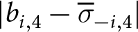 $|b_{i,4}-\overline \sigma_{-i,4}|$ in column (4). In columns (5) and (6), the dependent variable is the L1 distance between subjective expected payoffs (computed using reported beliefs) and objective expected payoffs (computed using observed action frequencies). High Own/Opponent Incentives correspond to indicators for whether the participant and their opponent face a high incentive level. 2 Steps and 3 Steps denote the different games in the experiment (see Figure 2). Controls refer to the participants’ socio-demographic characteristics. Heterocedasticity-robust standard errors are given in parentheses;
 $^*$,
 $^{**}$, and
 $^{***}$ denote p-values
 $ \lt 0.1$,
 $ \lt 0.05$, and
 $ \lt 0.01$, respectively.
Overall, higher own incentives tend to make beliefs both more sophisticated and more accurate, but these effects differ across games and across belief measures. Higher own incentives tend to shift beliefs toward attributing greater sophistication to opponents, especially in the simpler 2-Step game, and they improve several dimensions of belief accuracy. At the same time, beliefs about opponents facing higher incentives become harder to predict precisely. Thus, beliefs are an important part of the mechanism through which incentives affect choices. This motivates our next analysis of whether higher incentives also affect cognitive effort, as proxied by response times.
6. Incentives and response time
We proceed to examining whether incentive levels affect response time. Higher own incentives raise the marginal value of reducing mistakes and refining beliefs, and may therefore induce participants to devote more effort to the decision problem. If that additional effort takes the form of longer deliberation, one would expect response times to increase, as conjectured in Hypothesis 4a. We examine the mechanism underlying this hypothesis by regressing log response time on the incentive treatments, using the same baseline specification as before. Since greater effort need not always manifest itself in longer deliberation, we therefore interpret the analysis in this section as providing suggestive evidence on mechanism rather than a direct test of cognitive effort.
As Table 6 shows, higher own incentives increase response times substantially in both games: the log-point estimates are 0.38 in the 2-Step game and 0.37 in the 3-Step game, corresponding to increases of roughly 40-45%. Opponents’ incentives have a mixed effect. In the 2-Step game they have essentially no effect on response time, whereas in the 3-Step game they significantly increase response time by almost 20%. These patterns are consistent with the view that higher incentives increase the value of deliberation, although they should not be interpreted as showing that response time is itself a direct measure of cognitive effort. Relative to the existing literature, our findings are in line with the data in Alós-Ferrer and Buckenmaier (Reference Alós-Ferrer and Buckenmaier2021), where scaling up payoffs tends to increase response time in most variants of the 11-20 games discussed,Footnote 21 as well as with non-strategic evidence in Caplin et al. (Reference Caplin, Csaba, Leahy and Nov2020) and Enke et al. (Reference Enke, Gneezy, Hall, Martin, Nelidov, Offerman and van de Ven2023), where higher incentives increase response times, even though performance gains depend on task complexity.
Incentive level and response time (Hypothesis 4a)

Table 6 Long description
Regression results relate incentive levels to participants’ log response time in seconds for two games: 2 steps and 3 steps. Own incentives show a positive, statistically reliable association with longer response times in both games, with an estimated effect of 0.37 in each model (standard error 0.05). Opponent incentives are near zero and not statistically reliable in the 2-step game (0.03, standard error 0.05), but are positive and statistically reliable in the 3-step game (0.19, standard error 0.05). Both models include socio-demographic controls. Model fit is modest, with R squared 0.09 for 2 steps and 0.12 for 3 steps. Sample sizes are 837 for 2 steps and 877 for 3 steps. Estimates are associations from a regression with robust standard errors and should not be read as definitive causal effects.
Notes: This table reports the results of the regression specified in equation (1), where the dependent variable is the participant’s log response time (in seconds). High Own/Opponent Incentives correspond to indicators for whether the participant and their opponent face a high incentive level. 2 Steps and 3 Steps denote the different games in the experiment (see Figure 2). Controls refer to the participants’ socio-demographic characteristics. Heterocedasticity-robust standard errors are given in parentheses;  $^*$,
 $^{**}$, and
 $^{***}$ denote p-values
 $ \lt 0.1$,
 $ \lt 0.05$, and
 $ \lt 0.01$, respectively.
We then examine whether longer response times are associated with better performance, that is, whether longer response times are associated with (i) higher objective best-response rates and (ii) higher expected payoffs. As reported in Table 7, longer response times are indeed associated with a higher rate of best responses to opponent action frequencies (columns (1) and (2)) as well as an increase in expected payoffs (columns (3) and (4)). The association with expected payoffs is statistically strong but economically modest. The findings support Hypothesis 4b, although it is important to emphasise that the estimates here are associative rather than causal. Moreover, as in the existing literature, response time is an informative but imperfect proxy for cognitive effort, so the evidence in this section should be read as suggestive of mechanism rather than as a direct causal test of cognitive effort.
Response time, best responses, and payoffs (Hypothesis 4b)

Table 7 Long description
Regression results link log response time to two outcomes: objective best response rates and log expected payoffs, estimated separately for 2-step and 3-step games. Longer response times are positively associated with objective best responses in both games, with larger effects in the 2-step game (15.88) than the 3-step game (11.42). Longer response times also predict higher expected payoffs in both games (0.10 in 2-step; 0.06 in 3-step). Higher own incentives are positively related to both outcomes across games, with stronger effects in 2-step than 3-step (best responses 13.59 vs 8.46; payoffs 0.08 vs 0.03). Higher opponent incentives weakly increase objective best responses (5.50 in 2-step; 1.03 in 3-step, not statistically reliable) but reduce expected payoffs in both games, especially in 2-step (minus 0.14) compared with 3-step (minus 0.03). All models include demographic controls; model fit is modest (R-squared from 0.07 to 0.16) with sample sizes of 837 for 2-step and 877 for 3-step. Statistical significance is indicated by stars and standard errors are robust, so results describe associations rather than definitive causation.
Notes: This table examines the relation between, on the one hand, log response times (in seconds), and on the other objective best responses to the empirical frequency of opponents’ actions (columns (1) and (2)) and log expected payoffs, where expectations are taken also with respect to the empirical frequency of opponents’ actions (columns (3) and (4)). High Own/Opponent Incentives correspond to indicators for whether the participant and their opponent face a high incentive level. 2 Steps and 3 Steps denote the different games in the experiment (see Figure 2). Controls refer to the participants’ socio-demographic characteristics. Heterocedasticity-robust standard errors are given in parentheses;  $^*$,
 $^{**}$, and
 $^{***}$ denote p-values
 $ \lt 0.1$,
 $ \lt 0.05$, and
 $ \lt 0.01$, respectively.
We conclude with a descriptive analysis of how actions and beliefs vary with response time. For actions, we estimate a multinomial logit model relating choices to response time, incentive treatments, and individual characteristics, and then recover fitted choice frequencies as a function of response time by marginalising over the remaining covariates. For beliefs, we use nonparametric kernel regression to estimate the mean belief vector,  $b_i=(b_{i,1},b_{i,2},b_{i,3},b_{i,4})$, conditional on response time, incentive treatments, and individual characteristics. We then use the estimated conditional distribution to recover predicted mean belief distribution as a function of response time, holding the remaining covariates fixed at their sample means.
Figures 8 and 9 show how action probabilities and belief distributions change with response time, revealing two main patterns.Footnote 22 In the simpler 2-Step game, longer response times are associated with greater sophistication in both actions and beliefs. Panel (a) of Figure 8 shows that the predicted frequency of dominated actions,  $a_3$ and
 $a_4$, declines quickly with response time, whereas
 $a_2$ — the level-1 action — first mildly increases and then declines. Throughout, the frequency of choice of the level-2 action,
 $a_1$, increases monotonically in response time. Panel (a) of Figure 9 similarly shows that longer decisions are associated with lower beliefs in opponents choosing dominated actions and with higher beliefs in both the level-1 action (
 $a_2$) and the level-2 action (
 $a_1$). In the 3-Step game (panels (b) in Figures 8 and 9), we observe analogous patterns between actions and beliefs that correspond to the same level of sophistication. In actions there is a shift from the dominated action (
 $a_4$) and the level-1 action (
 $a_3$) toward the level-2 action (
 $a_2$), while play of the level-3 dominance-solution action (
 $a_1$) remains low and nearly flat. Belief in opponent dominated play is lower and belief in both level-1 and level-2 play is higher at later response times. Again a notable difference is that in the 3-Step game belief in dominance play — which corresponds to the level-3 action,
 $a_1$ — is lower for longer response times.
Action frequency and response time (a) 2-Step game (b) 3-Step game

Beliefs and response time (a) 2-Step game (b) 3-Step game

Fig 9 Long description
A line graph with the vertical axis label, Beliefs percent and tick labels 0, 10, 20, 30, 40, 50, 60. The horizontal axis label is Time, secs, with tick labels 15, 30, 60, 120, 240, 480. A legend below the plot reads, Action: 1, 2, 3, 4. Action 1 series: (15, 27), (30, 30), (60, 34), (120, 38), (240, 41), (480, 44). Action 2 series: (15, 31), (30, 35), (60, 39), (120, 44), (240, 47), (480, 50). Action 3 series: (15, 26), (30, 23), (60, 19), (120, 14), (240, 9), (480, 4). Action 4 series: (15, 18), (30, 14), (60, 10), (120, 6), (240, 3), (480, 1). The image B showing a line graph with the vertical axis label, Beliefs percent and tick labels 0, 10, 20, 30, 40, 50, 60. The horizontal axis label is Time, secs, with tick labels 15, 30, 60, 120, 240, 480. A legend below the plot reads, Action: 1, 2, 3, 4. Action 1 series: (15, 22), (30, 20), (60, 18), (120, 16), (240, 14), (480, 12). Action 2 series: (15, 30), (30, 32), (60, 34), (120, 36), (240, 38), (480, 41). Action 3 series: (15, 28), (30, 33), (60, 38), (120, 41), (240, 44), (480, 45). Action 4 series: (15, 20), (30, 16), (60, 11), (120, 7), (240, 4), (480, 2).
In short, the evidence suggests that faster decisions are associated with the intuitive level-1 actions and beliefs closer to uniform, whereas longer decisions are associated with fewer dominated choices, more weight on level-1 and level-2 opponent play, and a shift toward level-2 actions.Footnote 23 What does not increase with response time in the 3-Step game is the frequency of the level-3 dominance solution.
The estimation exercise and the positive relation between own incentives and response time point to a coherent mechanism. When own incentives are higher, the expected gain from reducing mistakes and refining beliefs is larger, so participants have a stronger incentive to invest in further reasoning. Consistent with this interpretation, higher own incentives are associated with longer response times, and longer response times are associated with more strategically sophisticated beliefs and actions. This is in line with models of sequential reasoning (e.g. Alaoui & Penta, Reference Alaoui and Penta2016; Gonçalves, Reference Gonçalves2024), in which players decide whether to exert additional cognitive effort by weighing its expected benefits against its cognitive costs.
7. Alternative explanations, robustness, and limitations of the findings
In this section, we discuss alternative explanations, robustness checks, and the natural limitations in interpreting the findings.
7.1. Alternative explanations
Although we cannot rule out all forms of other-regarding motives, the evidence suggests that they are unlikely to be the main driver of our findings. We sought to minimise confounding factors due to other-regarding preferences. As discussed in Section 2.2, we designed the experiment to reduce the scope for other-regarding preferences to mechanically account for the treatment effects, including through the choice of games, the way they are displayed, and the matching protocol. Moreover, many models of other-regarding preferences cannot generate behavioural changes from symmetrically scaling everyone’s payoffs (Charness & Rabin, Reference Charness and Rabin2002; Fehr & Schmidt, Reference Fehr and Schmidt1999; Levine, Reference Levine1998),Footnote 24 though asymmetric treatments could still matter if participants react to relative payoff differences.
A related concern is that participants assigned to low own incentives may become disappointed when their opponent has high incentives, and that this disappointment may lead to more random or less strategic behaviour. The data do not support this interpretation. If anything, choices are weakly more sophisticated, not less, when the opponent has higher incentives than when both face low incentives; see Figures 12b and 12d. In addition, even under low own incentives, participants best respond to their stated beliefs more than 40% of the time (Figure 5), well above the 25% rate implied by random choice, and this rate is stable relative to opponents’ incentives (Table 3).Footnote 25
7.2. Robustness checks
Participant pools: MTurk was the benchmark platform for online economics experiments in 2020, when the first experiment was run, whereas Prolific was the most common platform at the time of the replication. Online participant pools are particularly suitable for our purposes for two reasons. First, participants face a salient opportunity cost of time, as alternative paid tasks are readily available. This makes variation in incentives and response times especially meaningful. Second, online implementation avoids frictions that a laboratory setting would create for response-time analysis, since participants can complete and leave the task without having to wait for or disrupting others.Footnote 26
We conducted a robust replication in 2026 on Prolific.Footnote 27 Although there are some level differences across the two participant pools,Footnote 28 the treatment effects are consistent across MTurk and Prolific; see Appendix B.2.Footnote 29 We conclude the main findings hold across participant pools and are robust to a less salient presentation of the incentive manipulation.
Attention and understanding: Another possible concern is that our findings are driven by inattention and misunderstanding of the tasks. We took several steps to promote understanding: instructions were designed to be as clear and transparent as possible, participants could familiarise themselves with the interface during the instructions, and incentive levels were revealed only after the instruction stage, so attentiveness to the instructions should not differ systematically across treatments. The data also suggest that participants understood the task. Best-response rates to stated beliefs range from roughly 40-50% under low own incentives and 60-70% under high own incentives. These rates are comparable to those observed in laboratory studies with two- and three-action games (Costa-Gomes & Weizsäcker, Reference Costa-Gomes and Weizsäcker2008; Friedman & Ward, Reference Friedman and Ward2022; Nyarko & Schotter, Reference Nyarko and Schotter2002; Rey-Biel, Reference Rey-Biel2009). Moreover, the median time spent on the paid round was about one minute and the median time spent on the instruction page was 9 minutes, indicating that participants engaging seriously with both the instructions and the paid task.
At the end of the instructions, participants completed a comprehension quiz designed both to consolidate understanding and to emphasise the key aspects of the experiment; the median number of mistakes was two. Because all participants had to complete the quiz correctly before proceeding, the quiz ensured a minimum level of understanding. We nevertheless use initial quiz performance to assess whether the main results are driven by participants who at first misunderstood the task. In Appendix B.1, we reproduce the main regressions interacting the treatment indicators with the number of mistakes in the quiz. Initial quiz performance makes little difference to the qualitative conclusions and, if anything, the treatment effects are somewhat stronger among participants who made fewer mistakes.
7.3. Extreme incentives
Although higher incentives in our design tend to increase strategic sophistication, caution is warranted when extrapolating beyond the range of incentives we study. There may be an optimal level of incentives, deviations from which are detrimental to performance, as posited by the Yerkes and Dodson (Reference Yerkes and Dodson1908) ‘law’. As discussed by Camerer and Hogarth (Reference Camerer and Hogarth1999), for simple or well-learned tasks stronger incentives may lead to better performance, but extreme incentive levels can generate stress and impair cognition, limiting or even worsening performance. Ariely et al. (Reference Ariely, Gneezy, Loewenstein and Mazar2009) and Enke et al. (Reference Enke, Gneezy, Hall, Martin, Nelidov, Offerman and van de Ven2023) provide evidence that performance in individual decision-making tasks involving memory and reasoning can deteriorate under extreme incentives. In strategic settings, evidence on this phenomenon is more limited; if anything, extreme incentives have been found to shift behaviour toward benchmark equilibrium predictions in ultimatum bargaining (Andersen et al., Reference Andersen, Ertaç, Gneezy, Hoffman and List2011), a setting arguably strongly affected by cultural norms and other-regarding preferences.
In our design, the low incentive treatment was broadly in line with payment levels commonly used in related experiments, whilst the high incentive treatment substantially scaled those payments up but still remained within a realistic range. Our findings should therefore be interpreted as evidence about moderate incentive variation rather than about arbitrarily small or arbitrarily large stakes. The effect of scaling incentives, is likely to depend not only on the strategic environment, but also on the absolute level of incentives. At extremely low stakes, even large proportional changes may remain behaviourally negligible, and at very high stakes further increases may also have little additional effect or could even become counterproductive. That said, it is plausible that the main qualitative patterns we document — greater action and belief sophistication, better responses to stated beliefs, and longer response times — would continue to hold within a reasonable range.
8. Conclusion
This paper provides well-identified evidence that incentive levels affect behaviour in strategic settings. Higher own incentives reduce dominated play in both games. In the simpler 2-Step game, they also increase play of the dominance-solution action, corresponding to the level-2 action. In the more complex 3-Step game, however, they mainly shift behaviour away from dominated and level-1 actions toward the level-2 action, without increasing play of the dominance-solution action, which there corresponds to the level-3 action. Reported beliefs shift in a similar direction and also become more accurate along several dimensions. Choices and beliefs also react to opponent incentive levels in a consistent manner, although more weakly. At the same time, beliefs about opponents with higher incentives become less accurate, indicating that although higher opponent incentives shift behaviour in predictable directions, the magnitude of the effect is harder to predict than noisier play.
Response times provide suggestive evidence on mechanism. Higher own incentives are associated with substantially longer response times in both games, and longer response times are in turn associated with more sophisticated choices and beliefs. Faster decisions are concentrated on the intuitive level-1 action and on beliefs closer to uniform, whereas longer decisions are associated with fewer dominated choices, greater weight on level-1 and level-2 opponent play, and a shift toward level-2 actions. What longer response times do not deliver in the 3-Step game is an increase in play of the level-3 dominance solution.
In summary, the evidence points to two main channels through which own incentives affect strategic behaviour: a reduction in payoff-dependent mistakes and an increase in effort devoted to reasoning, for which response time provides an informative, though imperfect, proxy.
Two directions for future research seem particularly important. First, it would be useful to better understand the limits of incentives in fostering strategic sophistication, and how those limits depend on the complexity of the strategic environment. If, on the one hand, there is naturally a limit to what one can achieve in thinking about others’ behaviour through introspection alone, on the other hand such a limit surely depends on (or is informative about) how complex the environment is. This can shed light on what constitutes a simple strategic environment, which is a crucial consideration in designing successful mechanisms.
Second, response times deserve further attention in the study of strategic behaviour. They are often straightforward to collect and, as our results suggest, can be informative about both beliefs and choices. Further work developing game-theoretic models that incorporate response times, and establishing more systematically how response times relate to behaviour across environments, could significantly deepen our understanding of observed strategic behaviour.
Supplementary material
The supplementary material for this article can be found at https://doi.org/10.1017/eec.2026.10056.
Replication package
The data and code underlying this research is available on Zenodo at https://dx.doi.org/10.5281/zenodo.20609182.
Acknowledgements
We thank Larbi Alaoui, Marina Agranov, Guy Aridor, Alessandra Casella, Kfir Elias, Evan Friedman, Navin Kartik, Rosemarie Nagel, Ryan Oprea, Antonio Penta, Jacopo Perego, Silvio Ravaioli, Evan Sadler, Karl Schlag, Leeat Yariv, Michael Woodford, and the participants at Columbia, Essex, SWEET, the SAE Symposium, the EEA-ESEM Congress, the Barcelona Summer Forum, the ESA Conference, and the EAYE Annual Meeting for valuable comments. We are particularly grateful to Yeon-Koo Che, Terri Kneeland, and Mark Dean for their many insightful conversations. We are also indebted to the editor, Marta Serra-Garcia, and two anonymous referees whose comments and suggestions contributed significantly to improving this article. This material is based upon work supported by the National Science Foundation under Grant Number 1949395.


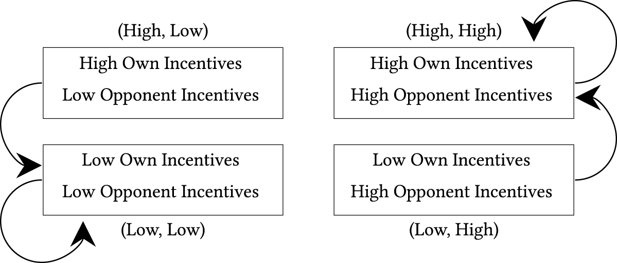
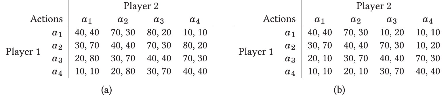


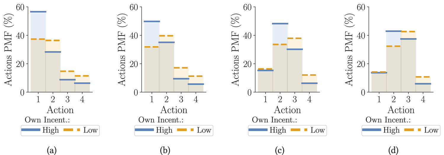
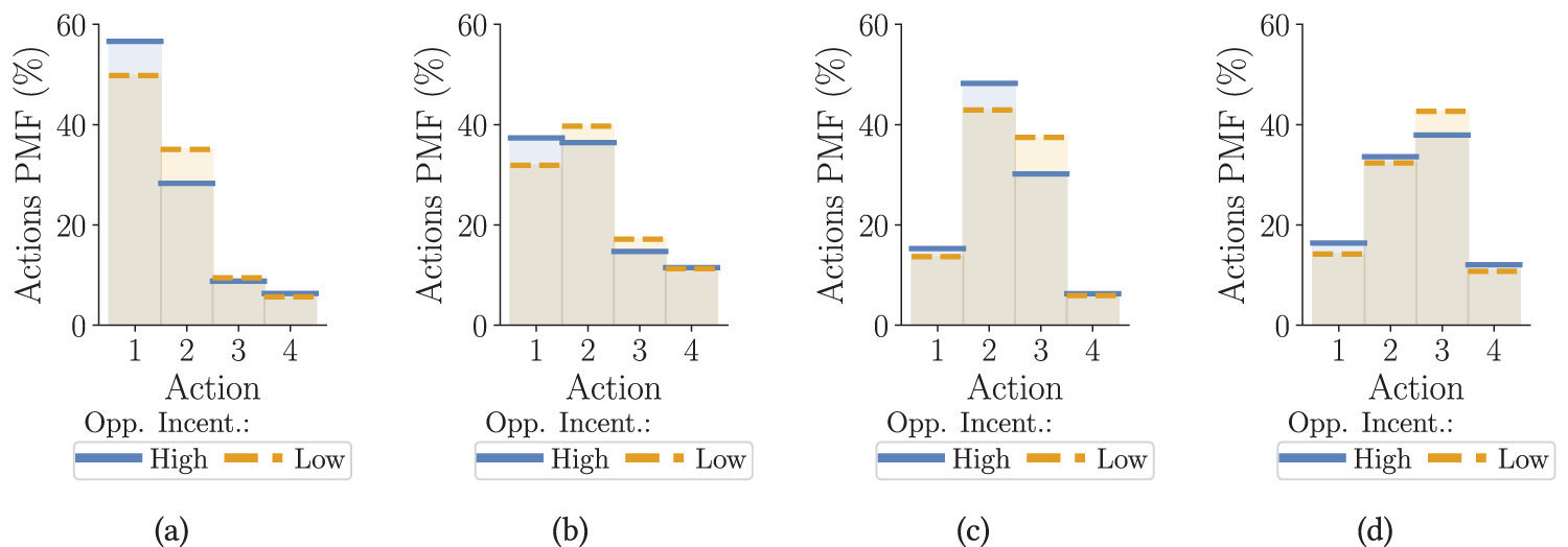

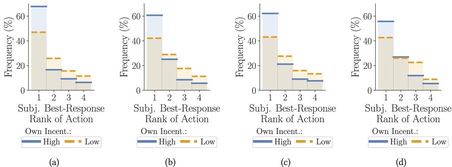
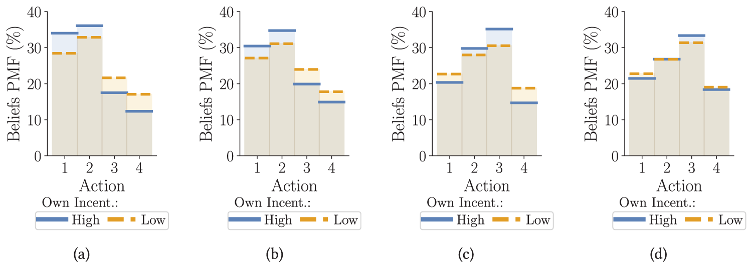
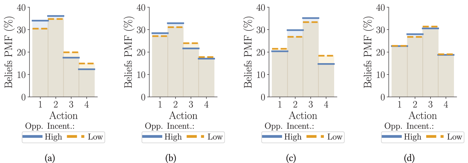


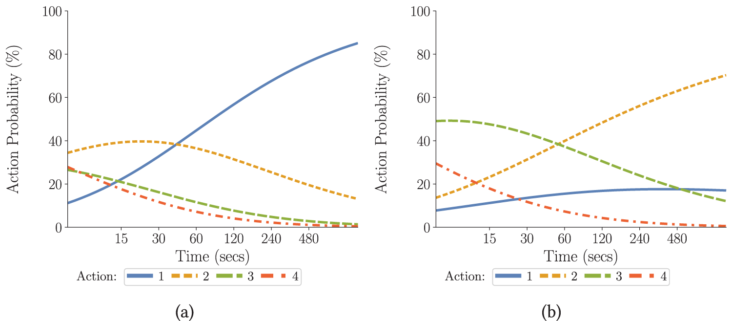
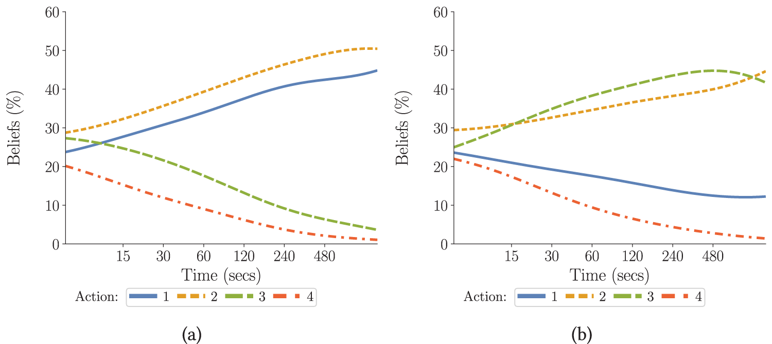


 Open access

