Perhaps Fiorina's remark is too gloomy, but it does seem apparent that the phenomenon of substantial turnout in large-scale electorates is anomalous for rational choice theory, in either its decision-theoretic or its game-theoretic guises. In a rough-and-ready sense, the problem is straightforward: In large electorates, the chance that any single voter will be pivotal is very small. Consequently, if voting imposes strictly positive costs, these will outweigh the expected gains from voting. Accordingly, rational citizens will not vote—contrary to the evidence. Hence, an anomaly.
This is the classical version of the turnout problem as formulated by Downs (1957). Downs's formulation, however, is decision-theoretic. In strategic models of turnout, if the cost of participating is not too high, then it will not be an equilibrium for everyone to stay home, for then a single voter could decide the election. The key insight of strategic models is that the probability of being pivotal is endogenous. That is, if citizens are rational, the voting decisions and pivot probabilities are determined simultaneously.
Strategic theories usually model turnout as a large team game (Palfrey and Rosenthal 1983, 1985). There are typically two alternatives (e.g., candidates) and two types of citizens (call them Democrats and Republicans), where each type or team has identical preferences. Preferences of each team are diametrically opposed. Each person can either vote, for either candidate, or stay home (shirk). Elections are decided by a simple plurality with some tie-breaking rule, usually a coin toss. All members of the winning faction earn a payoff for winning (whether or not they voted); losers get nothing. Independent of the outcome, citizens bear an additive and private cost of voting.
Strategic theories then solve for the equilibria of such team games. Because voting for the nonpreferred candidate is dominated for each voter, the relevant problem reduces to a participation game that simply involves the binary decision of whether to vote or stay home. The results of game theoretic models can be summarized as follows (Palfrey and Rosenthal 1983, 1985; Myerson 1998)
- No pure strategy equilibria exist, except in degenerate cases. For example, “Everybody votes” is an equilibrium only if voting costs are zero or if the teams are of exactly the same size.
- Many equilibria with positive turnout exist. Except in degenerate cases, these equilibria involve the use of mixed strategies by at least some voters.
- Equilibria with nontrivial turnout are asymmetric. That is, voters of the same type are required to use different strategies.
- High turnout equilibria are not robust to the introduction of uncertainty over either preferences and costs (Palfrey and Rosenthal 1985) or the number of players (Myerson 1998). The robust equilibria have vanishing turnout.
Thus, as Palfrey and Rosenthal (1985, 64) point out, “We have come full circle and are once again beset by the paradox of not voting.” The initial rough-and-ready intuition is still close to the mark: As long as all voters have strictly positive costs of voting, the expected turnout will be vanishingly small relative to the size of the electorate.
The term “paradox” here does not refer to a logical inconsistency or incompleteness. Rather, it indicates a puzzling implication of the rational choice theory of voting that is at odds with the facts.1
It is thus more appropriate to call it an “anomaly” in the sense of Kuhn (1962).
More precisely, the implication of vanishingly small turnout follows by
jointly assuming a certain behavioral model, such as expected utility maximization or Nash equilibrium, and making certain payoff assumptions as expressed, for example, in a normal form game: that voters care about outcomes and not, e.g., the act of voting per se, that voting is costly, and the like. Thus, a solution to the anomaly must modify either the behavioral model or the payoff assumptions or both.
The most prevalent response to this anomaly has been to modify the payoff assumptions. For example, citizens may have a sense of duty to vote that outweighs the cost of participation (Riker and Ordershook 1968).2
Empirically this may well be true, and we suspect that it does explain at least some turnout. But completely dispelling an anomaly in this manner raises obvious methodological concerns. To answer the question, “Why do people do
x?” by saying that people have a taste for
x seems theoretically shallow.
In this paper we take a different approach. We leave the game structure, and hence payoffs, alone, i.e., we assume that voting is costly, as in the classical models, and that voters are motivated by outcomes. Instead, we modify the rationality assumptions. Voters are not assumed to optimize. Rather, we assume that voters are adaptively rational: They learn to vote or to stay home. Their learning is a simple form of trial-and-error behavior that is consistent with basic axioms of reinforcement learning (Bush and Mosteller 1955): Actions that are successful today are more likely to be produced tomorrow; unsuccessful actions are less likely. This reinforcement learning is married to an aspiration level (Simon 1955), a threshold that partitions all possible current payoffs into satisfactory and unsatisfactory ones, hence indicating which actions are coded as successes (and so worthy of reinforcement) and which as failures (and so inhibited). A voter's aspiration level itself adjusts to experience, reflecting prior payoffs.
Our model thus proposes to use a synthesis of two of the most important competing research programs in political science: behavioralism and rational choice theory. As in the former, our model posits that decision makers are boundedly rational (Simon 1990): They adapt to a confusing, complex world by using (possibly suboptimal) heuristics such as trial and error. But as in the latter, our agents are embedded in a strategic environment—the interdependent world of elections—and we explicitly model some of the relevant connections by specifying a game form.3
This synthesis, which recently has made headway in economics, is sometimes called behavioral game theory. For an overview of this approach in economics, see Camerer 2003.
Supporting this synthesis entails taking a specific position on the intense controversies about paradigms that are so prominent in the discipline (e.g., Green and Shapiro 1994, Friedman 1996). Advocating a marriage may be foolish—partisans on both sides may dislike the offspring—but we are convinced that both of the older research progrrams have too much to offer political science to warrant rejecting either one. Game theory's substantive emphasis on strategic interdependence is a natural fit with most political contexts, and its methodological thrust (formal modeling) speeds the accumulation of knowledge by making it easy to criticize and revise our theories. On the other hand, behavioralism's emphasis on a psychologically accurate portrayal of how real political decision makers think, evaluate, and choose is too significant, empirically and theoretically, to be set aside.4
Indeed, we view the solution of the paradox of voting—important as it is in its own right—as primarily a vehicle for demonstrating the power of this new research program. We wish to demonstrate that political scientists need not be forced to choose between the substantively reasonable (behavioralism) and the analytically powerful (fullrationality game theory). And to make the case, what better arena than one that involves a core democratic process—elections—and that has exhibited an anomaly that has long plagued one of the parent programs? In short, much more is at stake than solving the paradox of voting.
The present paper is also synthetic regarding methods. Rational choice theorists usually work with mathematical models, deducing results “by hand” from axioms. Behavioralists in the Simonian tradition usually prefer computational models (e.g., Cyert and March 1963). We use both—for completely pragmatic reasons. As will be clear shortly, certain problems are best addressed analytically. But because of the model's complexity, we have turned to simulation to obtain many of our main results.5
The simulation results indicate that even if all the voters experience strictly positive costs of voting, turnout is substantial. Perhaps most strikingly,
turnout remains nonnegligible even when we increase the size of the electorate to 1 million voters. Moreover, the model implies some of the regularities from the empirical turnout literature, e.g., turnout is negatively correlated with participation costs or with differences in the relative sizes of factions. This is important because our approach not only proposes a solution to a hitherto unresolved puzzle, but also preserves the insights of existing models.
6 (As Lakatos [
1970] argued, a new research program demonstrates strong problem-solving power when one of its models solves a longstanding anomaly
and simultaneously continues to answer questions that the older research programs had successfully addressed.) Finally, we derive some new implications, such as a prediction of declining turnout in new democracies.
THE MODEL
Each agent has two choices, to vote or stay home (“shirk”).7
For an application to general finite normal form games see Bendor, Diermeier, and Ting n.d.
We assume that the electorate is of finite size
N and is divided into two blocs or factions, of
nD Democrats and
nR Republicans, with
nD > 0 and
nR > 0, and
nD+
nR =
N. (Candidates and their behavior are suppressed in the model.) Voters are denoted
i. Players interact at discrete time periods
t according to the same (one-shot) game.
Payoffs
As is typical of turnout games, the payoff to each player depends on the action taken by the voter, i.e., whether the voter participated or stayed home, and on the outcome of the election (and hence on the actions taken all by players, i.e., the action profile). Whichever side turns out more voters wins the election. Ties are decided by a (not necessarily fair) coin toss.
In addition to this conventional deterministic component, in our model payoffs have a random component. Let I ∈ {V, S} denote the actions of voting and shirking, respectively, and let J ∈ {W, L} denote the outcomes of winning and losing, respectively. We use πi,t(I, J) to denote agent i's realized payoffs at time t conditional on I and J, with corresponding random variables ΠI,J. Where convenient, we also use πi,t to denote agent i's unconditional payoff at time t.
To make our model as comparable as possible to earlier, game theoretic analyses, for the deterministic component we use the payoffs from the Palfrey–Rosenthal (1985) model. Thus πi,t(I, J) equals that game's normal form payoff plus a random shock [theta]i,t, where [theta]i,t is drawn from a mean-zero nondegenerate random variable that takes on finitely many values, and is i.i.d. across players and periods. As in the Palfrey–Rosenthal game, if player i is part of the winning faction, then she/he earns a deterministic payoff of bi > 0, whether or not she/he voted; all losers get zero. Player i's deterministic cost of voting is ci, where bi > ci > 0. Payoffs are additive in the benefits and costs. Thus for the deterministic component (and ignoring individual subscripts), winning voters get b − c; winning shirkers get b. Losing voters get −c; losing shirkers get 0. (Of course, the turnout paradox can be directly avoided by assuming that voters have a duty to vote or, equivalently, a “negative cost” of voting [Riker and Ordershook 1968]. In our model this corresponds to assuming that ci < 0. This will be investigated as a special case, below. Unless otherwise stated, however, we use the conventional assumption that voting is costly: ci > 0 for all i.)
Propensities and Adjustments
The heart of the model is the learning behavior of each agent. As stated above, adaptation combines reinforcement learning and endogenous aspirations. Thus in every period t, every actor i is endowed with a propensity (probability) to vote; call this pi,t(V) ∈ [0, 1]. That citizen's propensity to shirk is thus pi,t(S) = 1 − pi,t(V). For convenience, we often abbreviate the vote propensity to pi,t. Each citizen is also endowed with an aspiration level, denoted ai,t. Depending on pi,t, an action is realized for each i. This determines whether i's faction won or lost and whether i voted. Realized payoffs are then compared to aspiration levels, which may lead to the adjustment of propensities or aspirations for the next period.
In our model we wish to capture agents that learn by trial and error, i.e., propensities and aspirations may adjust to payoff experience. However, because an actor's attention may be on other matters, these codings do not invariably lead to adjustments in propensities. Consistent with the spirit of bounded rationality, we allow for the possibility that humans are sometimes inertial: They do not invariably adapt or learn. Thus with probability ∈p an agent does not adjust his/her propensity in a current period. Similarly, with probability ∈a an agent does not adjust his/her aspiration level. For simplicity we assume that ∈p and ∈a are mutually independent and i.i.d. across both agents and periods. We call any noninertial agent alert.
Propensities and aspirations may adjust randomly or deterministically. We assume that each agent has finitely many propensity levels; each agent's set of levels is fixed over time but agents' sets may differ. Agent i's propensities are denoted p1i,…, pil(i), with l(i) > 1. So p1i = pimin and pl(i)i = pimax. To represent random propensity adjustment we define for each i a family of random variables {Pi,t}t∈N with values drawn from p1i,…, pil (i ). Propensity adjustment then corresponds to a (stochastic) dynamic process. In deterministic adjustments (e.g., the Bush–Mosteller rule), one of the possible propensity values occurs with certainty; hence, such processes are a special case of this general stochastic approach.
As in the case of propensities we assume that each agent has finitely many aspiration levels; again, these are constant over time but may differ across individuals. Agent i 's feasible aspirations are denoted a1i,…, aim(i) with m(i) > 1. Again, we allow for random adjustment, with determinstic rules as a special case. Thus for each i, {Ai,t}t∈N is a family of (possibly degenerate) random variables with values drawn from a1i, …,aim(i). We assume that {Pi,t}t∈N and {Ai,t}t∈N are mutually independent stationary processes.When they adjust (i.e., when agents are not inertial), propensities as well as aspiration levels respond to experience, i.e., the payoffs received in previous rounds. We consider a very general class of adjustment rules for both propensities and adjustments. These assumptions on propensity and aspiration adjustment formally define our concept of an aspiration-based adjustment rule (ABAR).
Propensities
(P1) (positive feedback). For all i, t, and action I ∈ {S, V} chosen by i in t:
- if πi,t ≥ ai,t, then Pr(pi,t+1(I) ≥ pi,t(I)) = 1;
- if πi,t > ai,t and pi,t(I) < pimax, then Pr(pi,t+1(I) > pi,t(I)) = 1.
- (P2) (negative feedback). For all i, t, and action I chosen by i in t :
- if πi,t < ai,t, then Pr(pi,t+1 (I) ≤ pi,t(I)) = 1;
- if πi,t < ai,t and pi,t(I) > pimin, then also Pr(pi,t+1 (I) < pi,t(I)) = 1.
Aspirations
(A1) For all i,t:
- if πi,t > ai,t, then Pr(πi,t ≥ ai,t+1 > ai,t) = 1.
- (A2) For all i,t:
- if πi,t = ai,t, then Pr(ai,t+1 = ai,t) = 1.
- (A3) For all i,t:
- if πi,t < ai,t, then Pr(πi,t ≤ ai,t+1 < ai,t) = 1.
These assumptions formally capture the two central concepts of aspiration-based learning. The first key feature is feedback: (P1) says that if the payoff associated with an action taken exceeds the aspiration level (i.e., if it is coded as a success), its propensity will increase (if the agent is not inertial and the current propensity is not already maximal); (P2) says that if it is coded a failure, the agent's propensity to choose it in the future will decrease (if the agent is alert and the current propensity is not already minimal). The key second feature is the assumption of endogenous aspirations: Over time aspirations adjust to payoffs received (A1 and A3). (Note that because aspirations can adjust to experience, everyone's aspirations will be drawn toward the set of feasible payoffs.)
We can now describe a full cycle of learning. In each period t an agent is endowed with a vector of propensity levels pi,t and an aspiration level ai,t. Initially (i.e., for t = 1) these levels are assigned arbitrarily. Given the realized action of each agent, each agent receives a randomly drawn payoff conditional on the outcome of the election and the agent's own action. This leads to a propensity adjustment with probability 1 − ∈p and to an adjustment of the agent's aspiration level with probability 1 − ∈a. So, with probability ∈a∈p the agent is completely inertial. (An agent may be inertial regarding either propensities or aspirations or both.) Propensity adjustment occurs according to some adjustment process consistent with axioms (P1) and (P2). For aspiration adjustment, axioms (A1)–(A3) must be satisfied. This cycle is depicted in Figure 1.
The cycle of learning described by Figure 1 makes evident the differences between decision making in this model and the classical, full-rationality version. In the latter agents are relentlessly forward-looking and maximize expected utility, either in the decision-theoretic sense or in the strategic (Nash) sense. They understand every nuance of strategic interdependence—the Nash hypothesis—even in the presence of thousands of other decision makers (as in, e.g., large electorates). In our model decision making is driven by a process of backward-looking adaptation: If something worked in the past, become more inclined to use it today. This is a thoroughly psychological theory: Although agents respond to incentives, they do so myopically and crudely, without trying to optimize any function or deploy best responses to other people's strategies. Moreover, although they respond to experience (feedback), they are not Bayesians : e.g., they do not use Bayes's rule for computing posterior probabilities. Rather, their propensities merely obey the law of effect (Thorndike 1898), the foundation of psychological learning theory. Further, our model makes use of a cognitive concept—aspirations—that is foreign to the conceptual apparatus of rational choice theory. In the latter, agents care only about baskets of consequences and how these baskets compare to one another (i.e., their preference ordering). In contrast, in many psychological theories of choice (including ours), agents have internal standards or reference points by which they judge whether outcomes are good or bad, satisfactory or not. It is thus possible, for example, for a decision maker in a psychological theory to regard all outcomes in a choice situation as unsatisfactory. This has no meaning in expected utility theory; in our model it is not only a coherent idea, it can also lead to interesting predictions (see proposition 7, below).
Our model is naturally formalized as a discrete-time, finite-state Markov process. In any period, each agent has a vote propensity and an aspiration level. Hence, a state in this process is described by N pairs of propensities and aspirations—one pair for each of the N agents. Transitions between states are governed by a combination of the propensity- and aspiration-adjustment axioms and the payoff environment of the turnout game. Because these transitions are stationary—they do not depend on the date—we have a stationary Markov process.8
More precisely, we have a family of random variables {Xt : t ∈ N}, where Xt assumes values on the state space S = Xi=1…,NSi and Si consists of elements of the form (pi, ai) =:si. Generic states are thus of the form (pi, ai)i=1,…,N, denoted s. Note that given the independence assumptions on {Pi,t}t ∈N and {Ai,t}t∈N, Pr(Xt = s' | s) = Πi=1,…,N Pr(Xti = s'i | s), where {Xti} is the (decomposed) family of random variables assuming values on Si.
Our goal is to study the long-run behavior of this process. Using our definition of ABARs, we are able to derive the following important result about this proess. (Note that Proposition 1 does not require agents to use the same ABAR; it assumes only that they use
some stationary ABAR.)
9 Bendor, Diermeier, and Ting (2002) show that Proposition 1 extends to general normal-form games with finitely many agents and actions and heterogeneously distributed payoff shocks, provided the model satisfies two more properties. The first property describes the indirect effect of negative feedback when an agent has more than two feasible actions: (P3) For all i, t, and distinct actions I′ and I″, if i chose I' in t and πi,t (I′,·t) < ai,t, then Pr(pi,t+1(I″) > 0) > 0.Intuitively, if an action receives negative feedback, the propensity to play the other actions must increase. Note that (P2) implies (P3) if (as in the turnout game) each agent has only two actions.The second property stipulates that if one action receives agent i 's maximal propensity at any date t, then all of i 's other actions must get i 's minimal propensity in t. This is automatically satisfied in stage games with only two actions or if i 's maximal propensity equals one.
Proposition 1 (Bendor, Diermeier, and Ting 2002).
Suppose that players adjust by any arbitrary set of stationary ABARs. There are finitely many propensity values and aspiration levels. All payoff distributions are nondegenerate and finitely valued. Then the process is ergodic: It converges to a unique limiting distribution from any initial set of propensities and aspirations.
Ergodicity—reaching a unique limiting distribution, regardless of the initial values of the state variables—ensures the model's rich empirical content: Its prediction consists in a unique probability distribution. Moreover, many different variations of the adjustment process also ensure ergodicity (Bendor, Diermeier, and Ting 2002). That is, ergodicity is a robust property of our general model: It holds for many different specifications of randomness. In turn, some kind of randomness is vital for ergodicity. To understand both points, consider the following simple example. Suppose that initially all Democrats are fully disposed to vote and all Republicans are completely inclined to shirk. Then in the first period all Democrats vote while no Republicans do. Now suppose further that everyone's aspirations are low enough so that everyone is satisfied with their actions. Consequently they will start period 2 with exactly the same propensities they started with, and the whole process will repeat itself. In a deterministic model it follows that the Democrats' aspirations will stay low enough so that everyone will always get positive feedback for repeating their initial actions. So Democrats will always vote and Republicans never will. (Note that this holds even if there is only a single Democrat and millions of Republicans.) In general, in a deterministic model, if we rig the initial values of the state variables in the “right” way, we can get any extreme pattern of participation we desire. (In short, it would have a great many limiting distributions.) Thus the model would have too little empirical content: With the right auxiliary assumptions, it might be consistent with any observed pattern of turnout.10
This problem of impoverished empirical content can afflict any deterministic model of aspiration-based adaptation, as the following general result establishes. Because the result has negative implications for the predictive content of a class of models, it is similar to the folk theorems of repeated game theory. Theorem (Bendor, Diermeier, and Ting 2002). Consider any repeated game with deterministic payoffs and N ≥ 1 players. Suppose that the players adjust their action propensities by any arbitrary mix of rules that satisfy (P1) and adjust their aspiration levels by any arbitrary mix of rules that satisfy (A2). If each player's maximal propensity equals 1.0 and each player's feasible stage-game payoffs are a subset of his feasible aspiration levels, then any outcome of the stage game is a steady state, supported by some limiting distribution of the repeated game's underlying stochastic process.The result holds for any number of players, any number of actions, and asymmetric stage games. Moreover, agents can adapt by different rules, and can switch to different ways of adjusting propensities, provided only that new rules satisfy (P1). An analogous result holds for models with exogenously fixed aspirations. Indeed, many existing agent-based models fall under Theorem 1 and thus have little empirical content. See, e.g., Macy 1990, 1991, 1993 or Macy and Flache 2002.
The Computational Model
In most games of interst (including the turnout game) it is difficult or impossible to derive quantitative properties of the limiting distribution analytically. We therefore use simulation techniques, which enable us to examine the limiting distribution's important quantitative features, such as the average level of turnout. To use simulation we specify a particular computational model as a special case of the general model defined above. (The simulation program is described in the Appendix.)
Regarding payoffs, we simplify the general model in two ways. First, unless otherwise stated we assume homogeneous costs and benefits of voting: ci = c > 0 and bi = b > c, for all i. (Unless stated otherwise we normalize b to 1 in the simulation.) We also consider special cases in which members of one faction experience different costs or benefits than members of the other. In these, however, everyone in the same faction gets the same costs or benefits. Second, we assume that the random component, [theta]i,t, is distributed unitormly over [−ω/2, ω/2]. The parameter ω therefore represents the size of the support of the shock.
For our specific ABAR we use the well-known Bush–Mosteller reinforcement rule, which is defined as follows. If an actor who takes action I and happens to be noninertial in a given period codes the outcome as successful (i.e., if πi,t ≥ ai,t), then
where α ∈ (0, 1] represents the speed of learning or adaptation, given a successful outcome. Similarly, if the outcome was coded as a failure, then
where β ∈ (0, 1]. Finally, aspiration adjustment is implemented by stipulating that tomorrow's aspirations are a weighted average of today's aspiration level and today's payoff (Cyert and March 1963):
where λ∈ (0, 1).
Because we assume a finite state space—and hence finitely many propensity and aspiration values—these transition rules are approximate; we assume that actual values of pi,t and ai,t are rounded to three digits for all i and t.11
The rounding rule works as follows. To satisfy (P1)–(P3) and (A1)–(A3), we round up for all upward adjustment and round down for downward adjustment (when feasible). For example, if shirking did not satisfice in period t and pi,t(S) -βpi,t(S) = 0.306, then pi,t+1(S) = 0.300.
Thus this combination of adjustment rules is indeed a special case of an ABAR. For example, it specifies linear adjustment rules where ABARs in general are not restricted to a particular functional form. Moreover, Bush–Mosteller adjustments are deterministic, while the class of ABARs also includes probabilistic adjustment rules.
It is important to note that because the computational model satisfies all of the premises of the general model, Proposition 1 continues to hold: The simulation must indeed converge to a unique limiting distribution. Proposition 1 provides theoretical foundations for our simulations in two ways. First, because we know irrespective of the starting state the process will converge to the same limiting distribution, our simulation results do not depend on the initial state (provided, of course, the program is run “long enough”). Second, an alternative interpretation of the limiting distribution is that it also gives the long-run mean fraction of time that the process occupies a given state. Therefore, by considering a single run (for each parameter configuration) we can capture the limiting behavior of our process as if it were run for many different initial states.
However, the simulation approach is limiting in two ways. First, all simulation results depend on the specific functional form given by the Bush–Mosteller model and the specific payoff distribution. Second, any conclusion drawn from a simulation holds, strictly speaking, only for the chosen parameter configuration. To address both problems we derive analytical results for different classes of general ABARs and payoff distribtions to capture the general properties that drive the simulation runs.
MAIN RESULTS
Simulation Results
The main question obviously is, Will these adaptively rational agents learn to vote in significant numbers? The answer is “yes.” Run 1 (Figure 2) considers the case of 500,000 Republicans and 500,000 Democrats. Even in such a large electorate (well above that for congressional races), our model implies turnout of about 50%! As our finding of substantial turnout is perhaps the paper's central result, and one that may puzzle some readers, it is worthwhile to pause at this point to try to understand it. In an electorate of 1 million people, the chance that any one person will cast a pivotal vote is miniscule. Why, then, do so many people learn to vote? To see why, it is useful to study this “breakout of participation” in detail. Consider run 2 (Figure 3), in which citizens are initially very apathetic.12
By Theorem 1, our results are independent of the endogenous variables' starting values. However, examining low initial vote propensities provides valuable insight into the dynamics of the process. Also, henceforth we will study intermediate-sized electorates, of about 10,000 voters. As we discuss below, little is gained by considering much larger electorates, which take much longer to compute.
Nevertheless, participation quickly reaches about 50% and stabilizes at this level. The speed of this breakout of participation depends on the parameters. For example, when the adjustment parameter α is raised to 0.4, almost 50% of citizens vote in period 6.
13 Elsewhere (Bendor, Diermeier, and Ting 2001) we have shown that for symmetric and action-invariant Bush–Mosteller rules (these properties are defined below), the speed of convergence is increasing in α, the rate at which agents adjust their vote propensities. Thus, by choosing α appropriately, turnout can reach empirically reasonable levels after only a few elections.
The astute reader may have noticed that in the equal-faction size case, an equilibrium in pure strategies exists—with full turnout. So, perhaps the simulation simply captures voters coordinating on a high turnout state?14
Of course, if this interpretation were correct, one would need to explain why turnout levels do not converge to 100%.
A slight modification in our run shows that this is not the case. In run 3 (
Figure 4) factions are of almost-equal size (
nD = 5,000,
nR = 5,001).
Now a pure strategy equilibrium no longer exists. Nevertheless, turnout again stabilizes at about 50%.15
So ABARs do not necessarily converge to distributions that put a high probability on Nash equilibrium states. This insight generalizes to other games (Bendor, Diermeier, and Ting n.d.). For example, in the two-person prisoners' dilemma, agents using ABARs cooperate much of the time.
From now on we thus focus on the equal-faction case as a natural baseline and discuss the effect of relative faction size in a separate section below.
What causes this breakout of participation? Why do agents learn to participate? To understand what is going on it is very helpful to focus on the dynamics of a single hypothetical simulation. Suppose that nD = nR = 5,000, b = 1, c = 0.25, initial propensities are pi,0 = 0.01, initial aspirations are ai,0 = 0.5, and the size of the payoff support is 0.2. Suppose that Democrats win in period 1:50 D's vote and only 49 R's. The key question is, What happens to people's dispositions to vote after this election? Because everyone starts with intermediate aspirations, all the winning Democrats find winning and voting to be satisfactory. (Even with a bad random shock to payoffs, the worst payoff a winning voter can get is 0.65.) Hence these 50 Democrats are mobilized: Their vote propensities rise after the election.
However, the slothful behavior of their comrades, who enjoyed a free-riding payoff of between 0.9 and 1.1, is also reinforced. So this is not the place to look for the explanation of a major breakout of participation. The place to look is the effect that the Democratic victory had on their shirking opponents. The best payoff that a shirking Republican could get in period one was 0.1 (zero plus a maximally good shock). Because this is less than their initial aspiration level, all shirking losers are dissatisfied with staying home. Hence in the next period all such Republicans—the overwhelming majority of their team (4,951)—will increase their probability of voting. We call this loser-driven mobilization.
The story is not over. In period 2 the Republicans, having been mobilized by their loss in the previous election, will almost certainly win. The effect on their propensity to vote is complicated. All Republicans who actually voted will be reinforced for doing so, but all of their free-riding comrades will have that action supported as well. Thus, once again, focusing on the winners does not explain why the system eventually winds up at a much higher turnout level; once again, we must look at the losers—in this period, the Democrats. In period 2 almost all Democrats stay home and get a payoff of zero, on average. With aspirations adjusting slowly, and hence still close to one-half, the players will code payoffs that are about zero as failures. So now the Democrats' shirking is inhibited. Hence more of them turn out in period 3, and loser-driven mobilization continues. The mobilization of one side begets countermobilization, in a typically pluralist fashion.16
The mobilization and countermobilization amounts to an escalating arms race of effort that is collectively inefficient. The Pareto-optimal symmetric outcome is for everyone to stay home.
Finally, we can understand why participation breaks out in run 2 even though everyone begins with an aspiration level of −0.2. Even in the worst case a shirker cannot fall below a payoff of −0.1, hence all shirkers are satisfied with staying home in period 1. While one might think that this should stop the main cause of the breakout of participation, loser-driven mobilization, dead in its tracks, happy slothfulness does not—cannot —endure because aspirations adjust to experience. Thus, although either side is content to lose the election in period 1, that is only because we set their initial aspirations so low as to ensure this outcome. But aspirations are endogenous in this model, so they will not stay at this artificially low level. They will rise even if one's side loses—the expected payoff to a shirking loser is zero—and they will rise even more if one's party wins the coin toss and the election (for an expected payoff of one). And once a citizen's aspiration equals zero (as it does for many Republicans by period 4), shirking and losing will be dissatisfying over half the time. Thus, while shirking and winning continues to be fine, shirking and losing quickly becomes unsatisfactory. Once again, a process of loser-driven mobilization is triggered, as dissatisfied losing shirkers become more inclined to vote.
Explaining the “Breakout of Participation”: Analytical Results
Using our general model we now show in a step-by-step fashion why the mobilization observed in run 2 occurs. Indeed, we also show why much of it does not depend on the specific form of adaptation, the Bush–Mosteller mechanism, used in the simulation but is instead driven by much more general properties of trial-and-error learning. (For simplicity all of the following analytical results use the computational model's assumption of homogeneous costs and benefits of voting, except in those special cases where differences across factions are examined.)
The first result is exceedingly simple but it supplies the basis for what follows. Observation 1 reports a simple property about aspirations and electoral payoffs. We call a player's aspirations “not too high” if they are less than πV,Wmin and “not too low” if they exceed πmaxS, L, where the former denotes the minimal possible payoff from voting and winning and the latter is the maximal payoff obtained from shirking and losing. We also say that an actor is “satisfied” if the corresponding action is coded a success and “dissatisfied” if it is coded a failure.
Observation 1.
If in t the aspirations of people in the winning faction are not too high and the aspirations of people on the losing side are not too low, then all winners are satisfied by the outcome in t while all losers are dissatisfied.
This makes intuitive sense. Winners get payoffs of either πi,t(V,W) or πi,t(S, W), depending on whether they voted or stayed home. So if all winners have aspirations below πminV,W, then they are all content with the outcome. Similarly, losers get payoffs of either πi,t(V, L) or πi,t(S, L), depending on their individual choices. So if the aspirations of all losers exceed πmaxS, L, then losing is unacceptable.
Though simple, this condition is very important both substantively and analytically. Substantively, it identifies situations in which everyone's satisfaction is determined exclusively by the collective outcome: If your side wins, you are happy; if it loses, you are unhappy (Figure 5). An important special case of this condition is when all citizens have intermediate aspirations, in the interval (πmaxS, L, πminV,W). (In that case the conclusion of observation 1 holds if either party wins.) A natural interpretation of this special case is that people identify with the well-being of their factions: Personal satisfaction is driven completely by collective outcomes.
Now given the conditions described by observation 1 (which are satisfied by the initial conditions of run 3b), which citizens will mobilize after the election in period 1? That is, if observation 1 applies to period 1, which citizens will increase their propensity to vote in period 2? To answer that question one must make some assumptions about how propensities are adjusted. Of course, we could use the Bush–Mosteller mechanism employed in the simulation. Happily, however, the next result depends only on general qualitative properties of ABARs, and not on the specifics of the Bush–Mosteller rule. The next observation characterizes which citizens become more inclined to vote and which become less inclined.
Observation 2.
Suppose in t the aspirations of people in the winning faction are not too high and the aspirations of people on the losing side are not too low. If adjustment is by any arbitrary mix of ABARs, then all alert winning voters and all alert losing shirkers become more disposed to vote after the election in t (or remain fully disposed to vote). The other alert citizens become less inclined to vote (or remain fully inclined to shirk).
It is obvious that winning voters increase their propensity to participate: They voted and were pleased with the outcome. A bit less obviously, so will losing shirkers, as all losers were displeased with the outcome.17
We focus on these two sets of citizens because they typically determine whether mobilization will occur. Given realistic aspirations, winning shirkers and losing voters rarely become more likely to turn out: The former's apathy tends to be reinforced; the latter's participation, inhibited.
The next piece of the story involves political demography: How many citizens are either winning voters or losing shirkers? We say a win is “conclusive” if did not result from a favorable coin toss in the event of a tie.
Observation 3.
If in t the Democrats win (conclusively) and nD ≤ nR + 1 or the Republicans win (conclusively) and nR ≤ nD + 1, then the number of winning voters plus losing shirkers is a majority of the electorate in t.
To see why, suppose that the Republicans win. Hence we have more Republican (winning) voters than Democratic (losing) voters. But given that nR ≤ nD + 1, there must be at least as many Democratic shirkers as Republican ones.
Now let us combine observations 1, 2, and 3 to see how much of the electorate will, at the end of a given election, become more mobilized (increase their propensity to vote). It is important to note that the following result does not assume that everyone in the electorate uses the same type of adaptive rule. People may adapt in different ways and at different speeds, per observation 2. All that is required is that voters use some kind of ABAR.
Proposition 2.
Suppose that the following conditions hold: (i) In t the aspirations of people in the winning faction are not too high and the aspirations of people on the losing side are not too low; (ii) the election is conclusive and the winning party is not larger than the losing party by more than one voter; and (iii) everyone in t has a vote propensity of less than one. Then the expected number of citizens who become more disposed to vote exceeds the expected number who become less inclined.
Beyond the conditions of the three observations, the further requirement of proposition 2—before the election nobody is completely disposed to vote—is very mild. It is obviously satisfied by run 2, which presumes that initially everyone is almost completely inclined to shirk. Thus proposition 2 makes clear that outbreaks of participation are to be expected, if citizens learn via this large class of adaptive rules.18
Proposition 2 holds even if shirking by all citizens forms a Nash equilibrium. (In our game, universal pure shirking is Nash if c > b/2.) But Bendor, Mookherjee, and Ray (2001a) argue that the critical solution concept for stability in adaptive models is protected Nash equilibrium, where a unilateral deviation does not hurt other players. (For example, mutual defection in the two-person prisoner's dilemma is protected Nash.) Thus protected Nash equilibria are stable against random shocks: If player A trembles, B's propensity to play his Nash action is undisturbed. (See propositions 10 and 11 in Bendor, Mookherjee, and Ray 2001a.) This general idea applies directly to the present paper: Even when universal pure shirking is Nash, it is never protected Nash. (If a Democrat deviates from “all shirk,” then many other players—the Republicans—are hurt.)
Further, it is important to note that this result does not depend in any way on the size of the electorate. (Nor do any of our other analytical results, as we will see shortly.) In particular, proposition 2 does not require that the electorate be small. This gives us confidence that the results of run 1—stable, substantial amounts of turnout in a district with 1 million citizens—will generalize to even larger jurisdictions.
The notion of “loser-driven mobilization” that we discussed earlier falls naturally out of special cases of proposition 2. For example, consider circumstances in which initially everyone is fully disposed to shirk, as in run 2. Because aspirations are endogenous, they typically will increase rapidly into the intermediate region of (πmaxS, L, πminV,W). Once this happens, the run will satisfy all of the conditions of proposition 2, say in period t. Hence we know (analytically, now) that, on average, after the election in period t at least half of the noninertial citizens will become more inclined to vote. (As ties are very rare, typically more than half become more inclined.)
However, because no one initially has any inclination to vote and the speed of learning is relatively low (α = 0.1), relatively few people actually turn out in period t + 2. Given that winning voters and losing shirkers are over half the community, this implies that most of the newly mobilized are losing shirkers. Thus, in the early goings mobilization is loser-driven.
Proposition 2 establishes mobilization in a demographic or head-counting sense: When its assumptions are satisfied, more citizens will on average increase their propensity to participate than will decrease that tendency. This does not necessarily imply, however, that the electorate's average propensity to turn out rises. Whether that follows depends on how much those increasing their vote propensity boost their participation tendencies versus how much those decreasing reduce theirs. To flesh out this point, consider the following numerical example.
Let us reconsider run 2, in which all citizens started out with a vote propensity of only 0.01. Suppose that the Democrats won in the first period. Compare a Democrat (denoted D1) who voted and won with one who shirked (denoted D2). Because initial aspirations are low (−0.2), both of these Democrats are satisfied with their actions. Hence D1 will become more disposed to vote, while D2 will become more disposed to shirk. But now consider the magnitudes of their adjustments (given the Bush–Mosteller rule). Because D1's vote propensity was initially so low, D1's tendency to vote can rise substantially: The ceiling of 1.0 is a long way off. Quantitatively, with the speed of adjustment (α) set at 0.1, D1 will increase from 0.01 to 0.01 + 0.1(0.99) = 0.109: i.e., D1 will jump from almost-complete apathy to an approximately 10% chance of voting. But because D2 started with a shirk propensity of 0.99, the ceiling—the maximum feasible propensity—of 1.0 is very close. Hence D2 cannot become much more inclined to shirk. (Specifically, D2's shirk propensity increases from 0.99 to just 0.99 + 0.1(0.01) = 0.991.) Hence, although qualitatively D2's movement opposes D1's, with the former becoming more apathetic and the latter more mobilized, quantitatively D1's heightened mobilization swamps D2's increased lethargy. Indeed, in this example the district-wide average vote propensity would rise if more than 1% of the district became more mobilized.
In general, then, the ceiling effect is very powerful. Under symmetric Bush–Mosteller and many other adaptive rules, very high rates of shirking tend to be self-limiting: In these circumstances the satisfied shirkers cannot increase their shirk propensities much, while the propensities of satisfied voters have lots of room in which to rise.
Hence, once demographic mobilization is assured, e.g., via proposition 2, then the above per capita quantities constitute a sufficient condition for the electorate's average participation propensity to rise. To see which features of the Bush–Mosteller rule are crucial for the result to hold, we isolate and identify three properties of ABARs. For this purpose, the following notation will be useful. Let δi,t+(I,pi,t(I)) := E[pi,t+1 (I) | I succeeds] −pi,t(I), and δi,t−(I,pi,t(I)) := pi,t(I)-E[pi,t+1 (I) | I fails] represent the expected increment and decrement in propensities for success and failure, respectively. Now we can define the first property.
Definition
Suppose that pi,t′(I) > pi,t(I). The ABAR is weakly monotonic (with respect to action I) if δi,t+(I,pi,t′(I)) ≤ δi,t+(I,pi,t(I)) and δi,t−(I,pi,t′(I)) ≥ δi,t−(I,pi,t(I)).
Thus, for example, the expected increase in the propensity to vote, if it was tried and succeeded, is weakly decreasing in the current propensity to vote. (Henceforth we usually say just “monotonic” instead of “weakly monotonic.”)
Regarding the second property, note that with α = β in the Bush–Mosteller rule the degree of propensity adjustment is the same in the face of failure and of success. We can capture this “symmetry” feature in the following general property.
Definition
Suppose that pi,t′(I) = 1 - pi,t(I). The ABAR is symmetric (with respect to action I) if δi,t+(I, pi,t(I)) = δi,t−(I,pi,t′(I)).
Thus, given the same amount of adjustment room, symmetric ABARs adjust identically in response to failure and to success. It can be easily verified that Bush–Mosteller rules satisfy monotonicity and, with α = β, symmetry also. Their distinctive feature is linearity; i.e., their adjustment magnitudes are linear in the status quo propensity.
An ABAR that is both (strictly) monotonic and symmetric must display ceiling effects. Thus, if citizens use a monotonic and symmetric ABAR, then when citizens' participation propensities are already low the tendency to shirk cannot rise much more, whereas feedback that is favorable to voting can lead to big changes. And so the next result shows that the breakout of participation illustrated by run 2 holds for a rather large class of adaptive rules, under a broad range of parameter values. In particular, this generalization of Bush–Mosteller rules shows that their linearity plays no essential role in the outcome of the preceding example.19
We have extended Proposition 3 (Bendor, Diermeier, and Ting 2001) to cover asymmetric rules, which respond more to negative than to positive feedback. For evidence of this “negativity bias” see Baumeister et al. 2001.
Let
denote the district-wide average propensity to vote in t;
denotes its expected value.
Proposition 3.
Suppose that the following conditions hold: (i) In t the aspirations of people in the winning faction are not too high and the aspirations of people on the losing side are not too low; (ii) the election is conclusive and the winning party is not larger than the losing party by more than one voter; and (iii) everyone uses the same ABAR, which is monotonic and symmetric. If
for all i, then
.
Proposition 3 gives only a partial explanation of the outbreak of participation, because the antecedent specifies that all voters have a propensity of at most one-half. Of course, propostion 3 describes a sufficient condition for increasing average propensity to participate, not a necessary one. So it is consistent with run 2; i.e., it is consistent with the fact that mobilization continues in that run even after some pi,t(V)'s exceed one-half.
Because propensities (probabilistically) affect behavior, proposition 3 immediately implies that when its assumptions hold, expected turnout will rise. Because this conclusion is the payoff to the sequence of analytical mini-results that began with observation 1, it is worth recapitulating the sequence to get a clear overview of the logic that yields this conclusion. When observation 1 holds, aspirations are such that winners are happy and losers are sad. By observation 2, if everyone adjusts via some form of ABAR, then the noninertial winning voters and losing shirkers will become more disposed to vote (whenever that is possible). By observation 3, winning voters and losing shirkers groups are a majority of the electorate if (say) nD = nR. Hence it follows that if no citizen is fully disposed to vote in t and the conditions in observations 1–3 hold, then on average more people become more mobilized than become less mobilized, at the end of period t (proposition 2). If the district's current distribution of propensities is not so high as to evoke ceiling effects, then the demographic mobilization of proposition 2 in turn implies that the expected value of an electorate's average propensity to vote rises (proposition 3). Finally, because propensities are (probabilistically) related to behavior, expected turnout must also rise.
In sum, we see that run 2 does not depend on the details of the simulation program. Our results show that even at a starting point of nearly complete apathy, participation will break out eventually. The results of run 2 thus are the consequence of a few simple mechanisms that are instantiated by the parametric setting of this run. In this sense the analytical results also serve as a sweeping sensitivity test for that run. Instead of laboriously investigating a huge number of other parametric configurations, we can invoke the “if” part of a result and know that a finding stands up for all parameter values swept up by that clause. Deduction complements simulation.
WHY DOES MOBILIZATION STOP?
We know from the simulations reported thus far that mobilization does not continue indefinitely: It appears to level out at about 50% turnout. Why?
Given that behavior in our model is mediated by aspiration levels, the distribution of citizens' aspirations is very important. It is therefore no accident that the cornerstone of our analytical results, observation 1, pertains to aspirations. The hypothesis of observation 1 is that winners' aspirations are low enough so that winning is gratifying even if one paid the costs of participating, and losers' aspirations are high enough so that losing is dissatisfying even if one avoided those costs. Let us take up the hint inherent in observation 1 by examining what happens when we go to the opposite extreme: The aspirations of winning citizens are high, while those of the losers are low.
Proposition 4.
Suppose that pi,t(V) > 0 for all i. People adjust by any arbitrary mix of ABARs. If in t the winners' aspirations are in (πV,Wmax, πS, Wmin) and the losers' aspirations are in (πV, Lmax, πS, Lmin), then after the election all (noninertial) citizens will become less inclined to vote. 20
If (πmaxV,W, πminS,W) and (πmaxV,L, πminS,L) are empty, then Proposition 4 holds vacuously.
Obviously, given that everyone's propensity to vote decreases (or, due to inertia, remains unchanged), proposition 4 immediately implies that the expected value of the electorate's average propensity to vote falls.
Clearly, a situation in which all alert players are becoming more likely to stay home is unstable. Hence this one-sided domination cannot be a long-run probabilistic equilibrium. Something must give. What will give, we believe, is that the dominating faction will become too complacent: Too many will learn to free ride on their comrades' efforts. This will make the race competitive again.
Note that proposition 4 and its implications rest on very weak assumptions about the nature of trial-and-error learning: Only the qualitative properties of ABARs were assumed. Thus, citizens may differ substantially in how they learn.
What will produce aspirations of the type assumed by proposition 4? The proximate cause is that recently one faction has been winning by wide margins. Winning produces payoffs of either πi,t(V,W) or πi,t(S,W), and thus a sufficiently long string of victories will drive the winners' aspirations above πV,Wmax. Meanwhile, the corresponding long run of defeats will end the losers' aspirations below πS, Lmin.
What produces such one-sided strings? There are two main possibilities. If one side is much larger than the other, it will win many elections by virtue of size. (As we will see in the next section [below], changing the relative sizes of the factions in the simulation does affect turnout as this reasoning indicates.) Alternatively, if factions are relatively balanced one side might reel off a string of victories by chance. Thus, because aspirations adjust to experience and one side has been winning while the other has been losing, people in the dominant faction currently have high aspirations while members of the weaker party have low aspirations.21
Proposition 4 makes the restrictive assumption that all winners have high aspirations and all losers have low ones. This allows us to use the weak premise that people adjust via any arbitrary mix of ABARs. Stronger assumptions about adjustment rules would let us weaken the assumption about the distribution of aspirations.
The following result parallels proposition 3 by reversing some of its key assumptions and invoking the following property.
Definition
Suppose that pi,t(V) = pi,t′(S). The ABAR is action-invariant if δi,t−(V,pi,t(V)) = δi,t− (S,pi,t′(S)) and δi,t+(V,pi,t(V)) = δi,t+(S,pi,t′(S)).
Intuitively, an ABAR is action-invariant if the propensities to vote and to shirk are adjusted identically, given the same feedback (and thus independently of the action taken).
Proposition 5.
Suppose that everyone adapts via the same monotonic, symmetric, and action-invariant ABAR. Together, winners with aspirations in (πV,Wmax, πS, Wmin) and losers whose aspirations are in (πV, Lmax, πS, Lmin) are a majority in t. If
for all i, then
.
Naturally, proposition 5 implies that the expected turnout in t + 1 is less than that in period t. Thus, together propositions 3 and 5 give us a clear understanding of the dynamics of turnout in the simulation, given (for example) a start of nearly complete apathy. Initially, demographic mobilization and the ceiling effect—per capita amounts of propensity change—reinforce each other, as explained by observations 1–3: More people increase their propensity to vote than decrease it, and because they began with little inclination to participate, increasers have plenty of adjustment room, while decreasers have little. Eventually, however, mobilization is self-limiting because one or both of the underlying factors will reverse themselves. First, once the community's average propensity to vote exceeds one-half, the ceiling effect favors shirking: There is now more room to decrease than to increase. Second, one side may run off a string of victories, which will send some of the winners' aspirations above b - c and some of the losers below zero. If this happens to enough people, the demography of mobilization will turn around: Now a majority of people will become less inclined to vote. And so turnout will start to fall.
VARIATIONS IN PARTICIPATION
The main result of this paper is the emergence of substantial turnout in large electorates. That is, we propose a solution to rational choice theory's anomalous prediction of negligible turnout. However, rational choice models are successful in explaining variation in turnout (Hansen, Palfrey, and Rosenthal 1987; Nalebuff and Shachar 1999). Thus, we also need to consider whether the price of resolving the turnout anomaly is to lose the successful comparative static predictions of rational choice theory.
In comparative static analysis one analyzes how changes in the model's exogenous parameters (e.g., cost of participation) affect its endogenous variables (e.g., participation levels). In a probabilistic framework, on the other hand, we need to study how the properties of the (unique) limiting distribution (e.g., expected turnout) change as an exogenous parameter varies.
Variations in the Costs of Voting
Our model is consistent with a well-known empirical regularity: higher costs, lower turnout. (See runs 4a–4c, summarized in Table 1.) However, a substantial change in cost leads only to fairly moderate decrease in turnout. This perhaps surprising finding is an instance of a more general phenomenon in models of aspiration-based learning: The effects of changing payoffs on behavior are muted by aspirational mechanisms (March 1994). The reason is that aspirations adjust to experience—here, payoffs. Hence an increase in the cost of voting is partly absorbed by lower aspirations in the steady state.
When one faction has systematically higher costs of voting (due either to harassment by the other faction, as in the old South, or to more innocuous factors), one would expect that bloc to participate less in elections. That seems to be the case here (run 5; Figure 6). Run 5 spreads the factions' costs of voting apart from the common default value of 0.25. With the Democrats' cost of voting equal to 0.4, while the Republicans incur a cost of only 0.1, we see that by about period 1,000 only 10–13% of all Democrats are voting. It is more interesting to observe that Republican turnout is also falling below the values we saw in the benchmark cases of runs 1 and 2, even though their costs in run 5 are lower than in runs 1 and 2. Evidently this reflects an indirect influence of the higher Democrat costs: As Democratic participation is reduced, Republicans learn that they can stay home and still win. Generally in runs such as this the disadvantaged group will experience a rebound after their opponents stop voting. However, this recovery is brief as the advantaged group will quickly reassert itself, thus again producing the pattern observed in run 5.
Variations in Population and Faction Size
In game-theoretic models of turnout, participation quickly approaches zero as the population size increases. We already know from run 1 that this is not the case in our model. Nevertheless, participation is affected to some degree by N. Figure 7 presents the average participation levels for electorates of various sizes, at t = 1,000. Consistent with the data of Hansen, Palfrey, and Rosenthal (1985), our computational model predicts that turnout decreases in N.
Notice that the decline in turnout is nonlinear, dropping precipitously as N increases for N below 100. Turnout is significantly higher in small, committee-sized forums than in large legislative districts. The principal intuition behind this result is that pivot probabilities still matter (albeit experientially rather than prospectively): When N is small, each agent's likelihood of swinging the election is nontrivial. Thus, given realistic aspirations, voting is more likely to satisfice in an election with low N.
We have already noted (run 2) that very slight variations in the factions' relative sizes yield virtually the same patterns as the perfectly symmetric runs. However, if one faction becomes substantially larger than the other, then turnout in the steady state is noticeably lower (runs 6a, 6b, and 6c, summarized in Table 2). Further, over an empirically relevant range of proportions, the bigger the size asymmetry, the more participation falls. It is also intriguing to note that in runs 6a–6c the minority faction turns out at higher rates than does the majority faction.
Significantly, this decrease in turnout is accompanied by a polarization of aspirations: The majority faction's aspirations soar, while those of the minority plummet. Obviously, majority factions are winning most of the contests. This drives their aspirations up and the unfortunate minority's aspirations down.
Indeed, we claim that it is precisely this movement of aspirations out of the intermediate zone that causes vote propensities to fall. The explanation is the same as that put forward in the preceding section, where we explain why mobilization stops. A string of victories makes the majority complacent: Their aspirations go so high that only the highest payoff, winning and shirking, satisfices for many of them. (This holds probabilistically, because payoffs are stochastic.) Hence voting is inhibited, regardless of the electoral outcome, and the majority faction's average vote propensity falls. Meanwhile, the series of losses have reduced the minority's aspirations so much that for many of them losing and shirking has become acceptable. Thus shirking is reinforced, regardless of the electoral outcome, reducing the smaller group's average vote propensity.
This explanation is corroborated by two points, one computational and one analytical, relating the distribution of aspirations to participation rates. First, inspection of the simulation's dynamics reveals that as long as the aspirations remain intermediate (in the usual sense), average participation rates hold steady. They start to fall only when the aspirations of a substantial number of people in a faction begin to leave the intermediate zone.
Second, the following analytical result shows that this pattern holds more generally for Bush–Mosteller adjustments. In particular, proposition 6 implies that if aspirations remain intermediate, one-sided electoral competition does not systematically degrade participation propensities.
Proposition 6.
Suppose that either party can win conclusively in t. Citizen i uses an action-invariant Bush–Mosteller, and ai,t is intermediate.
(i) If pi,t ≤
, then E[pi,t+1] > pi,t.
(ii) If pi,t >
and the probability that i is pivotal in t is sufficiently low, then E[pi,t+1] < pi,t.
To see the intuition for proposition 6, consider an extremely lopsided district that has only one Republican (denoted R1) and many Democrats. Because everyone has intermediate aspirations, losing is unsatisfactory. Hence, because the Republican is virtually certain to lose, R1 is in what learning theorists call a malign environment: No matter what action R1 takes, the feedback is virtually sure to be negative. Thus if R1 is inclined to vote in t defeat will probably induce shirking, but if R1 is initially disposed to shirk defeat will probably induce mobilization. These probabilistic tendencies are amplified by the Bush–Mosteller's ceiling effects: If R1 is already inclined to vote, then not only is voting likely to be the action that is selected and then (probably) inhibited, but also an initially high vote propensity can be reduced greatly. Exactly the same quantitative effect holds for a minority citizen who is initially disposed to stay home. Consequently, Bush–Mosteller adaptation pushes a soon-to-be-defeated minority citizen with intermediate aspirations to dampen both initially apathetic and initially mobilized tendencies. Being outnumbered does not by itself systematically degrade participation; being outnumbered by a lot does.
Meanwhile, members of the majority faction in this lopsided district are in what learning theorists call a benign environment: No matter what action a Democrat takes, it is likely to be reinforced. Thus prior dispositions get strengthened: A Democrat who is already likely to vote at the start of period t will probably become still more mobilized, while one who is initially apathetic will probably become still more so. Hence no systematic degradation in the participation tendencies of majority faction citizens emerges either—as long as aspirations remain intermediate.
Decreasing Turnout in New Democracies
Thus far we have focused mainly on determinants of turnout that can be captured by game-theoretic models. The purpose was to demonstrate that our approach preserves the broad qualitative implications of rational choice models that are consistent with established empirical regularities. Already, however, we have seen that a behavorial model can lead to additional quantitative insights. For instance, the highly nonlinear nature of aspiration-based learning may either partially absorb exogenous changes (as in the case of changing costs of participation) or reinforce them (as in the case of large differences in faction size).
However, our model also yields qualitatively new inferences, by exploiting its somewhat richer psychological framework. Consider realistic versus unrealistic aspirations. The former are likely to prevail in stable democracies, in which citizens have learned which payoffs are feasible and which are utopian. But in a new or unstable democracy voters may have unrealistic aspirations; they may expect a new regime to transform society overnight.
Having unrealistically high aspirations—those exceeding the game's maximal payoff—can only produce disappointment. And if, in the excitement of building a new society, these unreasonable aspirations are initially coupled to high rates of participation, then disappointment leads to disillusionment with politics, i.e., to decreased political participation, as the next result shows.
Proposition 7.
Suppose that everyone uses the same monotonic and action-invariant ABAR. If ai,t > πS,Wmax and pi,t >
for all i, then
.
Of course, with unrealistically high aspirations, every action will be dissatisfying. But voting will tend to be inhibited more than shirking because of ceiling effects and the frequency of voting relative to shirking. Hence disillusionment with the results of a fledgling democracy can lower the average propensity to participate, and the expected turnout as well.22
We would like to thank Carole Uhlaner for suggesting this point.
The Duty to Vote
One response to the turnout anomaly was to change the payoff assumptions. The most influential of these attempts was Riker and Ordeshook's famous “D”-term, intended to capture a “duty to vote.” Formally, assuming a large enough D-term is equivalent to assuming negative costs of participation—whence participating is a strictly dominant strategy. Rational choice theory predicts that people would then always vote, but what happens in our model is surprising. Consider runs 7a–7c (Table 3), with run 4b included as a benchmark.
Comparing run 4b with run 7a we see that turnout does increase with negative costs. Yet it does not climb nearly as high as predicted by rational choice theory. That is, our aspiration-based model does not necessarily select strictly dominant actions. (As mentioned earlier this finding is not unique to the turnout game [see Bendor, Diermeier, and Ting n.d.].) This seems strange—until we recall the mediating effects of aspirations. In run 7a aspirations end up much higher than they were in 4b. Hence losing while voting is still usually dissatisfying. Consequently losing voters often become less inclined to participate, so full turnout cannot be a stable outcome even when participation costs are negative.
Aspiration-based models can imply even more surprising results. Consider run 7b, which is just like run 6a except that in this latest run the benefits of winning have been sharply reduced. Surprisingly, participation is higher when the benefits of winning are lower. Indeed, when we reduce b still further, to the point where people do not care about winning at all (run 7b), then citizens become almost fully disposed to vote!
What is going on here? Are runs 7a and 7b bizarre? Do they indicate that our simulation model is fundamentally flawed?
Not so: Far from being pathological, these runs illustrate a rather general effect. The counterintuitive effect that mobilization increases when the value of winning falls to zero is not peculiar either to the particular configuration of parameter values in runs 7a and 7b or to the functional forms of the simulation model. The next result will show analytically that patterns similar to those of the above runs can be derived under more general assumptions.23
For a more detailed analysis of the counterintuitive effects of aspiration-mediated change, see Bendor, Diermeier, and Ting n.d.
Note, in particular, that proposition 8 holds for
any b > −
c. Hence it does not matter how valuable winning is; the pure intrinsic motivation of civic duty leads to greater expected mobilization.
Proposition 8.
Consider two districts, A and B, with c < 0, such that in A, b = 0 (thus πSmax = πS,Wmax = πS,Lmax and πVmin = πV,Wmin = πV,Lmin), while in B, b > 0. Assume that p1i < pi,t < pl(i)i for all i. Then for any arbitrary collection of ABARs:
(i) If in district A <ai,t∈ (πSmax,πVmin), then pi,t+1 > pi,t with probability one for all alert citizens in A.
(ii) If πS,Wmin ≥ πV,Lmin, then the conclusion of (i) cannot hold for district B: For arbitrary faction sizes, pj,t+1 < pj,t with positive probability for any j in B.
(iii) If, in addition to the conditions of (i) and (ii), everyone in both districts uses the same symmetric and action-invariant Bush–Mosteller and
, then
.
Proposition 8 implies that if initially the districts start out with the same average vote propensity, then after period 1 the expected vote propensity in district A will exceed the expected propensity in B, at every date. The result is driven precisely by the fact that people in district A are motivated only by their sense of civic duty. As they do not care about the collective outcome, they have only two expected payoffs: −c > 0 for voting and zero for shirking. Because everyone's aspirations are realistic, in district A they will tend to be in (0, −c ). Hence for people in this district participating is always gratifying, while shirking never is. Consequently voting is always reinforced and shirking is always inhibited, regardless of the electoral outcome. Thus, in the case of degenerate payoff distributions, in district A everyone's propensity to turn out rises in every period until they reach 1, where they will stay. In contrast, in district B people care about winning. This implies that losing while voting can be disappointing. If this occurs—and such an outcome is always possible—then the losing voters will become less inclined to vote.24
Our result is consistent with the intriguing finding by psychologists that adding extrinsic rewards can impair the performance of actions for which people are already intrinsically motivated. For a review see Deci, Koestner, and Ryan 1999.
Note that proposition 8 holds for an extreme comparison, between a district where winning is worthless and one where winning is worth more than the private satisfaction of doing one's civic duty—yet, despite this, the district where winning is worthless has a higher expected turnout than the one where winning not only is worth something, but is the more important payoff.
EXTENSIONS AND CONCLUSIONS
This work attempts to construct a mathematical model of adaptively rational electoral participation. Specifically, the model
(a) implies substantial turnout even in very large electorates and even when voting is costly for all citizens;
(b) is consistent with most of the empirical regularities that determine levels of turnout; and
(c) provides new predictions, e.g., when voters feel a duty to vote or when their aspirations (in, for instance, new democracies) are unrealistic.
The results reported here are quite encouraging. Reinforcement learning, mediated by endogenous aspirations, seems to lead naturally to substantial turnout under a wide array of parametric configurations. Indeed, it has been hard to suppress participation in the computational model. Thus, we look forward to seeing the model subjected to systematic empirical testing (e.g., Kanazawa 1998, 2000).
Because adaptive learning models offer a behaviorally plausible assumption for voters in mass elections, applying them to contexts of multicandidate competition is a natural next step. Next on the agenda would be to introduce active (though still adaptive) parties or candidates (as in, e.g., Kollman, Miller, and Page 1992 or Bendor, Mookherjee, and Ray 2001b.)25
Such a model would correspond to an adaptive version of Ledyard 1984.
Payoffs to voters would then no longer be exogenously fixed; instead, they would depend on the platform adopted by the winning party. The present model and one of adaptive candidates would complement each other: The former depicts active voters while parties are passive; in the latter, candidates adjust their behavior while citizens do not (they always turn out and always vote sincerely). The logical next step is to combine both models into an integrated model of elections in which
both candidates and voters adaptively adjust their behavior. We propose (and have begun working on) a unified model of elections that synthesizes behavioralism and game theory. All agents in this model will be intendedly rational but not completely so; all will be tied together by the strategic interdependence created by electoral processes. We hope that this synthesis, by fusing the empirical insights of behavioralism to the analytical power of game theory, proves to be a fruitful way to study not only turnout but electoral processes in general.
APPENDIX
Simulation Program
Because of the serious tractability issues involved, we have written a program in ANSI C to simulate the described adaptively rational behavior. The program is compatible with the GNU C compiler and most UNIX operating system configurations. A version of this program is maintained at http://faculty-gsb.stanford.edu/formal_behavioralism.
We adopt the following terminology in describing the simulation results. A period is a one-shot play of the turnout game. A simulation is a sequence of periods, for a specific set of voters. Finally, a run is a collection of simulations.
When started, the program allows the user to set the following parameters before each run: (i) the number of simulations; (ii) the number of periods per simulation; (iii) the faction sizes, nD and nR; (iv) the payoff parameters, b and c; (v) the inertia probabilities, ∈a and ∈p; (vi) the reinforcement and inhibition rates, α and β; (vii) the aspiration updating rate, λ; (viii) the size of the payoff support ω; (ix) each faction's vote propensity at t = 0 (pi,0); and (x) each faction's aspiration level at t = 0 (ai,0).
When a run begins, the program initializes a pseudorandom number generator with an integer representing the current time. This standard procedure effectively ensures that each run's random parameters are independent of those of other runs. The program then initializes a custom data structure that keeps track of state variables (i.e., propensities and aspirations, which may change over the course of a run) and statistics related to the history of play.
In each period, moves are realized, given the underlying corresponding propensities. After payoffs are revealed, the data structure is updated to reflect the changed propensities and aspirations. These variables revert to their original values for each new simulation.
The data structure associated with each run can be used to recover statistics at different levels of a run. To reduce run times, only those statistics that are requested by the user are collected. In particular, the user may opt to view or save to disk any of the following: (i) the moves, payoffs, and adjusted propensities and aspirations after each period; (ii) the average and cumulative propensities and aspirations for each simulation, and a histogram of propensities for each voter for each simulation; (iii) the average propensities and aspirations across simulations for certain periods; and (iv) a histogram of final-period turnout and aspiration levels across simulations.
For the runs investigated in this paper, the final two items proved to be most useful. All of the run reports are composed of either time series of average turnout or histograms of final-period turnouts across simulations. While the program does not generate graphics on its own, the output files it creates are easily read into other programs for further processing.
The program is able to generate large samples of game play quickly, although naturally large electorates will slow run times considerably. Typical run times for most of the runs reported here (10,000 voters, 1,000 periods, and 1,000 simulations) ranged between 5 and 30 hours depending on hardware configurations.
Proofs
Before we prove the results described in the text, it is convenient first to state some facts about ABARs. (The proofs are available on request and are also given in Bendor, Diermeier, and Ting 2001.)
Fact 1
If all agents use the same ABAR, which is monotonic and action-invariant, and pi,t≤ (≥)
, then for all i and j (where i may or may not equal j): (a) δ+i(V; p) ≥ (≤) δ+j(S; 1 − p); and (b) δ−i(V; p) ≤ (≥) δ−j(S; 1 − p).
Fact 2
If all agents i use the same ABAR, which is monotonic and symmetric, and
for all i, then for all i and j (where i may or may not equal j) and
: (a) δ+i(V; p) ≥ δ−j(V; q); and (b) δ−i(S; 1 − p) ≥ δ+j(S; 1 − q).
Fact 3
If all agents use the same ABAR, which is monotonic, action-invariant and symmetric, and pi,t≤ (≥)
, then δ−i,t (S; 1 − p) = δ+j,t(V; p) ≥ (≤) δ−j,t(V; p) = δ+i,t(S; 1 − p).
Proof of Proposition 2.
Suppose that the Republicans win. Given the assumed aspirations, a Republican victory produces satisfied Republicans and dissatisfied Democrats. Hence, because everyone adjusts by some kind of ABAR, noninertial Republican voters and alert Democratic shirkers will increase their propensity to vote. Given that observation 3 applies, Republican voters plus Democratic shirkers must exceed Republican shirkers plus Democratic voters. And because the probability of inertia is i.i.d. across voters, the expected number of noninertial Republican voters and Democratic shirkers exceeds the expected number of alert Republican shirkers and Democratic voters. Exactly the same logic holds for the other case. QED
Proof of Proposition 3.
Consider first winning noninertial voters, who increase their participation propensities, versus losing alert voters, who decrease theirs. We know that there are more of the former, in expectation. Fact 2 shows that none of these per capita expected increases can be less than any of the expected decreases. Hence the net expected effect of the changes of these two groups must be to increase the expected value of the district-wide average propensity to vote.
Now compare the losing noninertial shirkers, who decrease their propensity to shirk, with the winning alert shirkers, who increase theirs. The expected number of the former exceeds the expected number of the latter, given the assumptions of the proposition. Hence we need only check that the losing alert shirkers' per capita expected decreases are at least as big as the per capita expected increases of the winning alert shirkers. This is also ensured by Fact 2. QED
Proof of Proposition 4.
Suppose that the Democrats win. Given the realized payoffs and the assumed aspiration levels, Democratic shirkers are satisfied but Democratic voters are not. Similarly, Republican shirkers are content but Republican voters are not. By the definition of ABARs, all satisfied (alert) shirkers will increase their propensity to shirk and all dissatisfied (alert) voters will decrease their propensity to vote. QED
Proof of Proposition 5.
Any shirking winner whose aspiration is “realistically high”—i.e., in (πmaxV,W, πminS,W)—must be content with shirking, while any voting winner with aspirations in the same interval must be dissatisfied with voting. Similarly, any shirking loser whose aspiration is “realistically low”—i.e., in (πmaxV,L, πminS,L)—must be content with shirking, while any voting loser with aspirations in the same interval must be dissatisfied with voting. Hence, given the demographic assumption of proposition 6, the expected number of people who will become more apathetic (or remain completely apathetic) exceeds the expected number who will become more mobilized (or remain completely mobilized).
It suffices to show that the expected increase in the shirk propensity of all those becoming more apathetic must exceed the expected increase in the vote propensity of all those becoming more mobilized. This is established by Fact 3. QED
Proof of Proposition 6.
This proof is quite long and is therefore omitted. It can be obtained from the authors on request and can also be found in Bendor, Diermeier, and Ting 2001.
Proof of Proposition 7.
Because
to show that E[pi,t+1] < pi,t it suffices to show that pi,t(pi,t − δ−i,t(V)) + (1 − pi,t) (pi,t + δ−i,t (S)) < pi,t, which (after rearranging terms) holds if and only if δ−i,t (S) < pi,t [δ−i,t (V) + δ−i,t(S)]. But given pi,t >
and Fact 1 we have δ−i,t(V) > δ−i,t(S); hence E[pi,t+1] < pi,t for every i. QED
Proof of Proposition 8.
(i) Because b = 0, the electoral outcome has no effect. Hence the sign of feedback depends only on individual behavior. And if ai,t ∈ (πmaxS, πminV) for all i, then shirking is dissatisfying while voting is satisfying. Given that every agent i is using some kind of ABAR and pi,t < pl(i)i, if i is alert, i will become more inclined to vote.
(ii) Because pi,t ∈ (0, 1) for all i, every kind of outcome can occur: i can vote or shirk and either win or lose. If ai,t ≤ πminS,W, then consider the event (which occurs with positive probability) in which i shirks and wins, and πi,t > πminS,W. Then i's propensity to shirk rises, if i is alert. If ai,t > πminS,W, then consider the event (which also occurs with positive probability) in which i votes, loses, and gets πminV,L. Since πminV,L ≤ πminS,W < ai,t, this is dissatisfying; so if i is alert, his/her vote propensity falls.
(iii) Because everyone in district A is either inertial or becomes more inclined to vote, and everyone uses the same symmetric and action-invariant Bush–Mosteller rule,
Suppose, counterfactually, that all alert citizens in B would increase their vote propensity with probability one. Because they use the same symmetric, action-invariant Bush–Mosteller rule, then (given the counterfactual)
. Now it is given that
, and hence,
. And given (ii), any j in B becomes, with positive probability, less disposed to vote. Hence, it follows that
. QED



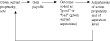
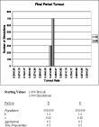
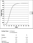
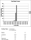
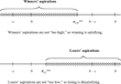
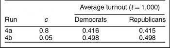
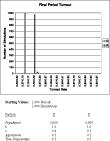
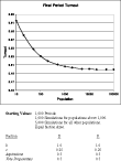
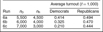
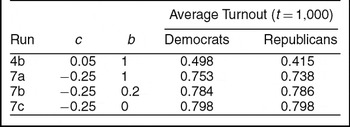



Comments
No Comments have been published for this article.