1 Introduction
1.1 Energy dissipation
Some 2 TW (i.e.
 $2\times 10^{12}$
W) of energy is needed to maintain the stratification of the ocean by diapycnal mixing (Munk & Wunsch Reference Munk and Wunsch1998; Garrett Reference Garrett2003; Wunsch & Ferrari Reference Wunsch and Ferrari2004). Since the total mass of the ocean is approximately
 $1.4\times 10^{21}$
kg, this amounts to approximately
 $1.4~\text{nW}~\text{kg}^{-1}$
(i.e.
 $1.4\times 10^{-9}~\text{W}~\text{kg}^{-1}$
). Although apparently minute, the rate of energy loss required to sustain stratification is a major control on ocean circulation, and has led to a search to identify the global distribution of energy sources and sinks and the connecting energy pathways and processes. The breaking of internal waves is commonly assumed to be the dominant processes in the downscale transfer of energy to turbulence, mixing and dissipation (e.g. Garrett Reference Garrett1979; Wunsch & Ferrari Reference Wunsch and Ferrari2004; Waterhouse et al.
Reference Waterhouse, MacKinnon, Nash, Alford, Kunze, Simmons, Polzin, St Laurent, Sun and Pinkel2014; Meyer et al.
Reference Meyer, Sloyan, Polzin, Phillips and Bindoff2015). By ‘wave breaking’ is meant a turbulent process initiated by internal waves that leads to a loss of their energy and directly to diapycnal mixing, the transfer of mass and momentum across isopycnal surfaces of constant density. This therefore excludes a loss of wave energy from an internal wave to other waves or modes of motion that occurs without the generation of turbulence, for example by resonant waves (Phillips Reference Phillips1966) or wave–vortical mode interactions (Lelong & Riley Reference Lelong and Riley1991).
The total dissipation of tidal energy in the deep ocean is known to be approximately 1 TW (Egbert & Ray Reference Egbert and Ray2001), much of which is transferred from the tidal waves to short internal waves in regions of rough topography and subsequently supposed to be dissipated by internal wave breaking (Nikurashin & Legg Reference Nikurashin and Legg2011). The global pattern of tidal mixing in the deep ocean is described by St Laurent, Simmons & Jayne (Reference St Laurent, Simmons and Jayne2002), while Eden & Olbers (Reference Eden and Olbers2014) model the global propagation and dissipation of internal tides and near-inertial waves scattered by rough topography. A further 0.2 TW of energy comes from the conversion of largely wind-driven geostrophic flows (mean flows and mesoscale eddies) into internal waves in the lee of bottom topography (Nikurashin & Ferrari Reference Nikurashin and Ferrari2013). These waves are also thought subsequently to surrender their energy and contribute to mixing by breaking (Meyer et al. Reference Meyer, Sloyan, Polzin, Phillips and Bindoff2015). Additional contributions to the net dissipation come from the downward radiation and subsequent breaking of internal waves, particularly internal near-inertial waves, generated by wind stress and heat transfer in the upper ocean boundary layer (Alford & Gregg Reference Alford and Gregg2001; Thorpe Reference Thorpe2010a ; Cuypers et al. Reference Cuypers, Le Vaillant, Bouruet-Aubertot, Vialard and McPhaden2013). Together these various contributions to the internal wave field are sufficient to support the required rate diapycnal mixing.
The mean energy of the internal wave field, neglecting internal tides, is
 $3.8~\text{kJ}~\text{m}^{-2}$
(i.e.
 $3.8\times 10^{3}~\text{kg}~\text{s}^{-2}$
) averaged over the mean ocean depth of approximately 3800 m (Munk Reference Munk, Warren and Wunsch1981). The energy per unit mass that may be available for transfer to turbulence through wave breaking is therefore approximately
 $1\times 10^{-3}~\text{J}~\text{kg}^{-1}$
(i.e.
 $1\times 10^{-3}~\text{m}^{2}~\text{s}^{-2}$
, approximately the kinetic energy of water with speed 3–
 $4~\text{cm}~\text{s}^{-1}$
. Because of the dominance of near-inertial internal waves the kinetic energy in the wave field is approximately three times greater than the potential energy). If a typical value of the mean rate of dissipation of turbulent kinetic energy per unit mass is chosen to be
 $1.4\times 10^{-9}~\text{W}~\text{kg}^{-1}$
(i.e.
 $1.4\times 10^{-9}~\text{m}^{2}~\text{s}^{-3}$
) to account for the 2 TW of dissipation required to maintain the ocean’s stratification, and if this is supplied by the breaking and loss of energy through internal waves with no replenishment of the internal wave energy, the time scale for the removal of internal wave energy is approximately
 $6.9\times 10^{5}$
s,
 ${\approx}8$
days.
Although there is growing evidence that mixing is enhanced in ‘hot spots’, for example near rough or sloping topography (Polzin et al.
Reference Polzin, Toole, Ledwell and Schmitt1997; Nikurashin & Legg Reference Nikurashin and Legg2011; Lamb Reference Lamb2014; Waterhouse et al.
Reference Waterhouse, MacKinnon, Nash, Alford, Kunze, Simmons, Polzin, St Laurent, Sun and Pinkel2014), attention here is focussed on the mixing caused by wave breaking and mixing in mid-water. The rate of supply of wave energy from the surface and the seabed is limited by the vertical group velocity of internal waves, typically approximately
 $1~\text{cm}~\text{s}^{-1}$
, making it possible, if perhaps marginal, that replenishment of energy to internal waves in mid-water from these sources can be achieved in 8 days. Further supplies of internal wave energy are, however, also available: the loss of energy by internal tides generated at and radiating from the continental slopes or oceanic ridges (Alford & Zhao Reference Alford and Zhao2007; Eden & Olbers Reference Eden and Olbers2014) and by mesoscale eddies (Nikurashin & Ferrari Reference Nikurashin and Ferrari2013).
1.2 The objectives
Much of the attention on internal waves as a pathway to dissipation has focussed on the supply of energy to the waves of small scale because they appear more likely to break, making their energy available for mixing. (This excludes internal tides except at locations where they encounter continental slopes and form fronts; Thorpe (Reference Thorpe1987), van Haren & Gostiaux (Reference van Haren and Gostiaux2010).) The total energy within the small scale internal waves in mid-water appears sufficient to support the required mixing there provided that it is lost locally in diapycnal transfer processes and is not, in a substantial part, radiated away, to be lost in breaking on continental and island slopes or transferred from the internal wave field by processes not involving wave breaking. Our objective is to assess the efficiency and effectiveness of wave breaking in mid-water as a pathway to the mixing and dissipation of energy by estimating the rate of energy dissipation by breaking internal waves in mid-water. Can the mixing induced by internal wave breaking supply sufficient energy to drive the mixing required to support the ocean stratification? Is there sufficient information about internal wave breaking to answer this question?
1.3 Internal wave breaking
Disregarding double-diffusive convection, there are two known primary processes through which diapycnal mixing is driven in the ocean: convective (or Rayleigh–Taylor) and shear-induced Kelvin–Helmholtz instability (KHI). Both can be associated with breaking nonlinear internal waves. The first may occur when waves are steep enough to produce overturning isopycnal surfaces and the second when sufficient shear is produced by the waves to reduce a local gradient Richardson number to a value less than some critical value, commonly less than 0.25.
1.3.1 Convective instability
Convective instability and the production of interacting buoyant plumes and subsequent turbulence (Turner Reference Turner1973) arises from the formation of regions of high Rayleigh number static instability through the folding of isopycnal surfaces by internal waves. This includes the class of progressive internal wave breaking described by Orlansk & Bryan (Reference Orlansk and Bryan1969), the breaking of standing internal waves Thorpe (Reference Thorpe1994a ) and the breaking of progressive waves in an accelerating shear flow (see Thorpe (Reference Thorpe2005); § 5.6.2). Convective overturn is observed in the core of solitary waves on the continental shelf (Lamb Reference Lamb2014; Zhang & Alford Reference Zhang and Alford2015) and as vertically propagating internal waves encounter a critical layer, as illustrated in laboratory experiments (e.g. Thorpe Reference Thorpe1981; Koop & McGee Reference Koop and McGee1986).
1.3.2 Kelvin–Helmholtz instability, KHI
The stages of transition to turbulence in KHI are described in detail by Mashayek & Peltier (Reference Mashayek and Peltier2012) and Salehipour, Peltier & Mashayek (Reference Salehipour, Peltier and Mashayek2015). KHI and the production of billows and braids represent a known type of progressive internal wave breaking in the ocean (Smyth & Moum Reference Smyth and Moum2012). The development of the instability has been observed in the Mediterranean thermocline by Woods (Reference Woods1968), in solitary internal waves on the continental shelf (Moum et al. Reference Moum, Farmer, Smyth, Armi and Vagle2003; Zhang & Alford Reference Zhang and Alford2015; Carr et al. Reference Carr, Franklin, King, Davies, Grue and Dritschel2017), in laboratory experiments by Troy & Koseff (Reference Troy and Koseff2005) and numerically by Fringer & Street (Reference Fringer and Street2003). KH billows have also been recorded by van Haren & Gostiaux (Reference van Haren and Gostiaux2010) some 15 m above the sloping sides of the Great Meteor seamount during the downslope-flowing phase of the internal tide.
1.3.3 Wave breaking in mid-water
In all the cases referred to in the preceding two sections, the observed breaking waves occur principally on density interfaces. There appear to be no definitive observations of breaking of internal waves in a relatively uniform density gradient representing that of the mid-water ocean. Some of the most detailed observations of mixing are those made by Alford & Pinkel (Reference Alford and Pinkel2000) to a depth of approximately 400 m off the central California coast (35
 $^{\circ }$
N, 121
 $^{\circ }$
W) from the research platform, FLIP, moored in 1.5 km deep water. These show an increased likelihood of overturning isopycnal surfaces in the presence of small (5–20 m vertical scale) internal waves and sometimes, but not always, where the Richardson number is small. On the basis of a study of internal wave spectra, Garrett & Munk (Reference Garrett and Munk1972) argue that, except at great depths where the buoyancy frequency,
 $N$
, is very small, shear instability is very much more likely than convective overturning to cause waves to break because fewer root mean square (r.m.s.) wave-induced shears are required to reduce the gradient Richardson number to the Miles–Howard limit of 0.25 than the number of r.m.s. wave slopes required to produce convective overturns. There are however no theoretical studies of the development of instability in the time dependent flow of internal waves in uniformly stratified fluids.
Turbulence in the ocean is sporadic and intermittent (Gregg Reference Gregg1980; Kunze & Sundermeyer Reference Kunze and Sundermeyer2015), and the flow preceding and leading to its onset in local regions can be expected to be anomalous. It will not, for example, be that characterised by the spectrum of internal waves, or even by individual waves described by or consistent with the mean spectral energy corresponding to their frequency. Breaking leading to turbulence is likely to occur only in relatively exceptional and rare wave conditions. It is probable that, like waves on the sea surface (Donelan, Longuet-Higgins & Turner Reference Donelan, Longuet-Higgins and Turner1972), some of the internal waves that break in the mid-water ocean will belong to propagating wave groups and, for example, repetition of their breaking will reflect this (Thorpe Reference Thorpe1999a , Reference Thorpe2010a ). It is likely that breaking occurs as a consequence of there being greater wave amplitude, isopycnal slope or wave-induced shear at some location, moving in time, within a wave group, augmented by the presence of the ambient wave field through which the group is passing (i.e. by wave superposition); local conditions of high isopycnal slope, favouring convective instability, or a sustained low gradient Richardson number, leading to KHI, are reached and, if conditions persist, small disturbances grow and cause turbulent mixing.
1.4 Content and arrangement
A fundamental assumption of the adopted models is that, in the local regions where mixing is about to occur, the flow can be represented by the exact, finite amplitude, internal wave solution of the equations of motion. This solution is described in § 2.1. Before being relaxed in § 5, it is further supposed that, although the regions in which turbulence is about to occur may vary in structure and the ocean contains internal waves with a broad spectral range of steepness and frequencies, all the waves representing the flow just prior to the onset of mixing (and which, to produce turbulence and mixing, are about to break) have the same (anomalous) steepness and frequency.
The methodology for estimating energy loss in breaking waves is described in §§ 2.2 and 2.3. A novel parameter is introduced in § 2.4 to help assess the energy lost in mixing. Denoted by the symbol
 $\unicode[STIX]{x1D6EC}_{I}$
it is defined as the mean area of the fronts of internal wave breaking regions per unit volume, and has therefore dimensions of (length)
 $^{-1}$
. Mixing causes local changes to the vertical density and velocity profiles, resulting in a loss of energy from the waves representing the local flow field and the transfer of some of their wave energy to turbulence. The two classes of wave breaking, by convective or KH instability, are discussed in §§ 3 and 4, respectively. The energy dissipated by turbulence is calculated and this, and other measures of wave mixing, are compared with data obtained in mid-water in the Pacific that are described in § 2.5 and later referred to as ‘GS’. For readers who do not wish to see all the details of the analysis, summaries of §§ 3 and 4 are provided in §§ 3.4 and 4.4, respectively.
The main results are reviewed in § 6. The study of energy transfer is supported by seven appendices. In appendix A comparison is made of the density profiles caused by the convective instability of internal waves and the vortex-produced density pattern of overturns modelled by van Haren & Gostiaux (Reference van Haren and Gostiaux2014). In §§ C.1 and D.1 estimates are made of the times required for convective and KH instability to develop in steady flows. These are compared with the times for which conditions for instability are maintained in the variable flow field of an internal wave. If the latter are significantly longer than the former it may be assumed that, in relation to the changes in flow caused by the wave, instability may be taken as instantaneous or that the wave field may be regarded as frozen during the transition process. The generation of vortices or pancake eddies by breaking internal waves is considered in appendix G.
2 Energy loss by internal waves
2.1 The breaking wave model
A simple but precise representation of finite amplitude progressive internal waves is adopted to describe the flow field just as it becomes unstable and mixing commences: in the Boussinesq approximation, an exact solution of the governing equations is available that describes internal waves of frequency,
 $\unicode[STIX]{x1D70E}$
, propagating through a uniformly stratified fluid of constant buoyancy frequency,
 $N$
, and density
 $\unicode[STIX]{x1D70C}_{0}(1-N^{2}z/g)$
and zero mean flow (Thorpe Reference Thorpe2005; § 2.3.2). The horizontal,
 $x$
,
 $y$
, and vertical,
 $z$
, components of velocity are
 $$\begin{eqnarray}\displaystyle u=(s\unicode[STIX]{x1D70E}/k)\cos \unicode[STIX]{x1D701},\quad v=(sf/k)\sin \unicode[STIX]{x1D701}\quad \text{and}\quad w=-(s\unicode[STIX]{x1D70E}/m)\cos \unicode[STIX]{x1D701}, & & \displaystyle\end{eqnarray}$$
respectively, where the wavenumber is (
 $k,m$
),
 $\unicode[STIX]{x1D701}=(kx+mz-\unicode[STIX]{x1D70E}t)$
is the wave phase,
 $a$
is the wave amplitude,
 $s=am$
is defined as the wave steepness,
 $\unicode[STIX]{x1D70C}_{0}$
is the mean fluid density and
 $f$
is the Coriolis frequency. The maximum slope of isopycnals is
 $s\tan \unicode[STIX]{x1D703}/(1-s)$
, where
 $\tan \unicode[STIX]{x1D703}=k/m$
. In the wave-perturbed flow the density is
 $$\begin{eqnarray}\displaystyle \unicode[STIX]{x1D70C}=\unicode[STIX]{x1D70C}_{0}[1-(N^{2}/g)(z-a\sin \unicode[STIX]{x1D701})], & & \displaystyle\end{eqnarray}$$
and
 $$\begin{eqnarray}\displaystyle \text{d}\unicode[STIX]{x1D70C}/\text{d}z=-\unicode[STIX]{x1D70C}_{0}(N^{2}/g)(1-s\cos \unicode[STIX]{x1D701}). & & \displaystyle\end{eqnarray}$$
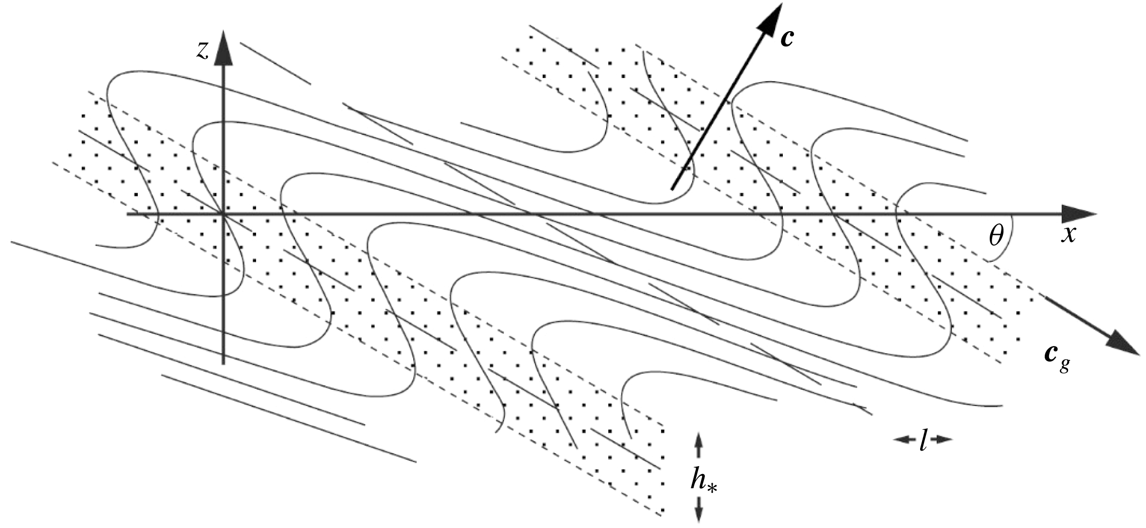
An example of the waves is shown in figure 1. The fluid density and velocity fields are similar on surfaces of constant phase,
 $\unicode[STIX]{x1D701}$
, lying at angle
 $\unicode[STIX]{x1D703}$
to the horizontal.
Isopycnal surfaces perturbed by an internal wave with
 $s=1.5$
and
 $\unicode[STIX]{x1D703}=30^{\circ }$
, those surrounding
 $x=z=0$
representing the local density field at the onset of convective instability and turbulence. Stippled regions show sloping regions of wave overturn and static instability occurring over a height,
 $h_{\ast }$
, that are produced in the density field by wave motions when
 $s>1$
. The directions of the phase,
 $\boldsymbol{c}$
, and group velocity,
 $\boldsymbol{c}_{g}$
, are indicated. The horizontal extent of overturns is
 $l$
.

For simplicity (and until the constraint is relaxed in § 5) it is now assumed that the waves representing the local flow in which turbulence is about to occur are all of the same steepness,
 $s$
, and frequency,
 $\unicode[STIX]{x1D70E}$
; in this model only such waves contribute to mixing. To cover their full range of variation, it is generally sufficient to examine the variation of critical features than control the stability of the flow (such as the slope of isopycnals or Richardson number) with the phase,
 $mz$
, over one vertical wavelength at
 $x=0$
and
 $t=0$
. This is appropriate provided that the wave-induced flow represents the local flow field at the onset of instability. If
 $s>4.712$
, the maximum density in the wave field near
 $x=0$
may be exceeded in an overlying location (above a height
 $2\unicode[STIX]{x03C0}/m$
, Thorpe (Reference Thorpe1994b
); see § 3.1 later) and unless the actual flow has similar properties, the local fit is appropriate only within one wavelength surrounding
 $x=t=0$
.
The extreme local values of isopycnal slope or small Richardson number that result in the breaking of individual waves advance through the fluid at the velocity,
 $\boldsymbol{c}_{b}=\boldsymbol{c}+\boldsymbol{c}_{g}$
(Thorpe Reference Thorpe1999a
), and
 $\boldsymbol{c}_{b}$
is generally different from either the phase velocity,
 $\boldsymbol{c}$
, or the group velocity,
 $\boldsymbol{c}_{g}$
, which are at right angles to one another (Mowbray & Rarity Reference Mowbray and Rarity1967). The magnitude of the speed of advance of the internal wave breaking region is found to be
 $c_{b}=N/K$
, where
 $K=(k^{2}+m^{2})^{1/2}$
is the wavenumber of the breaking wave, or
 $$\begin{eqnarray}\displaystyle c_{b}=Nm^{-1}\cos \unicode[STIX]{x1D703}. & & \displaystyle\end{eqnarray}$$
The angle,
 $\unicode[STIX]{x1D703}$
, is the inclination of the group velocity to the horizontal as shown in figure 1. The wave frequency is given by the dispersion relation,
 $$\begin{eqnarray}\displaystyle \unicode[STIX]{x1D70E}^{2}=N^{2}\sin ^{2}\unicode[STIX]{x1D703}+f^{2}\cos ^{2}\unicode[STIX]{x1D703}, & & \displaystyle\end{eqnarray}$$
where
 $f$
is the Coriolis parameter. The vector
 $\boldsymbol{c}_{b}$
is inclined at an angle
 $\unicode[STIX]{x1D703}_{b}=-\tan ^{-1}(F^{2}\cot \unicode[STIX]{x1D703})$
to the horizontal, where
 $F=f/N$
. The breaking region is consequently nearly horizontal if
 $F^{2}\ll \tan \unicode[STIX]{x1D703}$
or when
 $\unicode[STIX]{x1D70E}\gg f$
. The wave-induced motion is then predominantly in the
 $x$
–
 $z$
plane, the case considered in § 3. For the near-inertial waves with
 $\unicode[STIX]{x1D70E}\approx f$
considered in § 4, the angle,
 $\unicode[STIX]{x1D703}$
is small and
 $\unicode[STIX]{x1D703}_{b}$
may differ substantially from zero.
2.2 The energy of the internal waves
The energy in the wave field is of importance because, in the process of breaking, it provides the energy of the turbulent flow. The potential energy of the wave-disturbed density field described by (2.2) relative to
 $z=0$
integrated over one vertical wavelength and per unit horizontal area at the horizontal location and time of breaking,
 $x=t=0$
, is
 $$\begin{eqnarray}\displaystyle g\unicode[STIX]{x1D70C}_{0}\int _{-\unicode[STIX]{x03C0}/m}^{\unicode[STIX]{x03C0}/m}[1-(N^{2}/g)(z-a\sin mz)]z\,\text{d}z=-(2\unicode[STIX]{x1D70C}_{0}N^{2}\unicode[STIX]{x03C0}/3m^{3})[\unicode[STIX]{x03C0}^{2}-3s]. & & \displaystyle\end{eqnarray}$$
The terms in the last expression contain two contributions,
 $$\begin{eqnarray}\displaystyle PE_{m}=-(2\unicode[STIX]{x1D70C}_{0}N^{2}\unicode[STIX]{x03C0}^{3}/3m^{3}) & & \displaystyle\end{eqnarray}$$
from the ambient density,
 $\unicode[STIX]{x1D70C}_{0}[1-(N^{2}z/g)]$
, within which a wave is propagating, and
 $$\begin{eqnarray}\displaystyle PE_{w}=(2s\unicode[STIX]{x1D70C}_{0}N^{2}\unicode[STIX]{x03C0}/m^{3}) & & \displaystyle\end{eqnarray}$$
derived from the wave-induced perturbation of density. In the Boussinesq approximation, the corresponding local kinetic energy of the wave is
 $$\begin{eqnarray}\displaystyle KE_{w} & = & \displaystyle (\unicode[STIX]{x1D70C}_{0}/2)\int _{-\unicode[STIX]{x03C0}m}^{\unicode[STIX]{x03C0}/m}[u^{2}+v^{2}+w^{2}]\,\text{d}z\nonumber\\ \displaystyle & = & \displaystyle (\unicode[STIX]{x1D70C}_{0}N^{2}s^{2}\unicode[STIX]{x03C0}/2m^{3})[1+2(F\cot \unicode[STIX]{x1D703})^{2}],\end{eqnarray}$$
there being none from the (zero) mean flow.
The kinetic energy of the internal waves per unit mass (or the kinetic energy density) is found by integration over one vertical (
 $-\unicode[STIX]{x03C0}/m$
to
 $\unicode[STIX]{x03C0}/m$
) and one horizontal (0 to
 $2\unicode[STIX]{x03C0}/k$
) wavelength at
 $t=0$
and division by
 $\unicode[STIX]{x1D70C}_{0}$
:
 $$\begin{eqnarray}\displaystyle KE_{w}^{\ast } & = & \displaystyle (\unicode[STIX]{x1D70C}_{0}/2)\int _{0}^{2\unicode[STIX]{x03C0}/k}\int _{-\unicode[STIX]{x03C0}/m}^{\unicode[STIX]{x03C0}/m}[u^{2}+v^{2}+w^{2}]\,\text{d}z\,\text{d}x/(4\unicode[STIX]{x1D70C}_{0}\unicode[STIX]{x03C0}^{2}/km)\nonumber\\ \displaystyle & = & \displaystyle (N^{2}s^{2}/4m^{2})[1+2(F\cot \unicode[STIX]{x1D703})^{2}].\end{eqnarray}$$
The potential energy density per unit mass is
 $$\begin{eqnarray}\displaystyle PE_{w}^{\ast }=N^{2}\int _{0}^{2\unicode[STIX]{x03C0}/k}\int _{-\unicode[STIX]{x03C0}/m}^{\unicode[STIX]{x03C0}/m}(\unicode[STIX]{x1D702}^{2}/2)\,\text{d}z_{0}\,\text{d}x/(4\unicode[STIX]{x03C0}^{2}/km), & & \displaystyle\end{eqnarray}$$
where
 $\unicode[STIX]{x1D702}(x,z_{0})$
is the displacement of isopycnals from their level
 $z_{0}$
in the ambient density profile,
 $\unicode[STIX]{x1D70C}=\unicode[STIX]{x1D70C}_{0}(1-N^{2}z/g)$
, and is given by
 $$\begin{eqnarray}\displaystyle \unicode[STIX]{x1D702}=a\sin [kx+m(z_{0}+\unicode[STIX]{x1D702})] & & \displaystyle\end{eqnarray}$$
(Thorpe Reference Thorpe1968a ). The mean wave energy per unit mass is
 $$\begin{eqnarray}\displaystyle E_{w}^{\ast }=(PE_{w}^{\ast }+KE_{w}^{\ast }). & & \displaystyle\end{eqnarray}$$
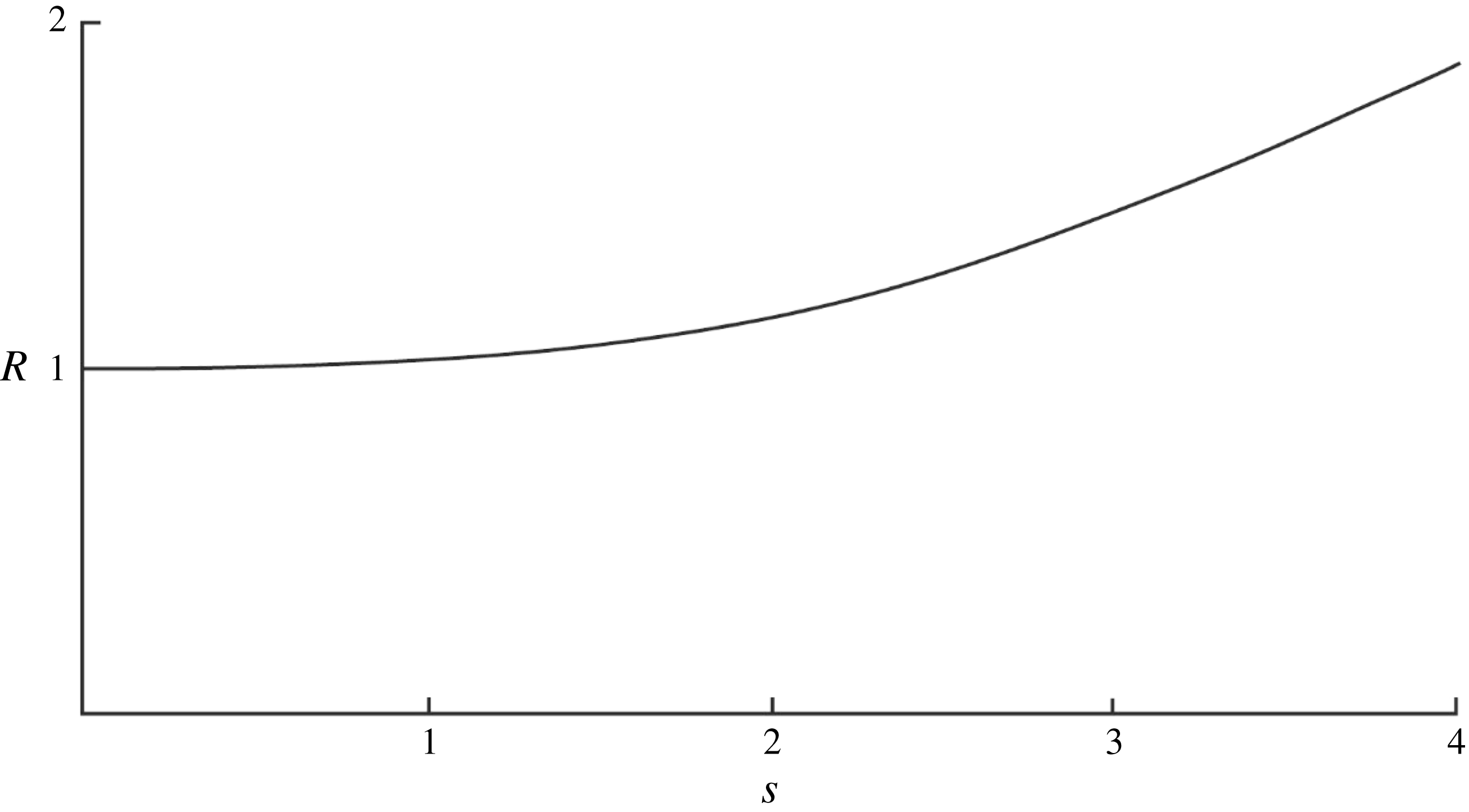
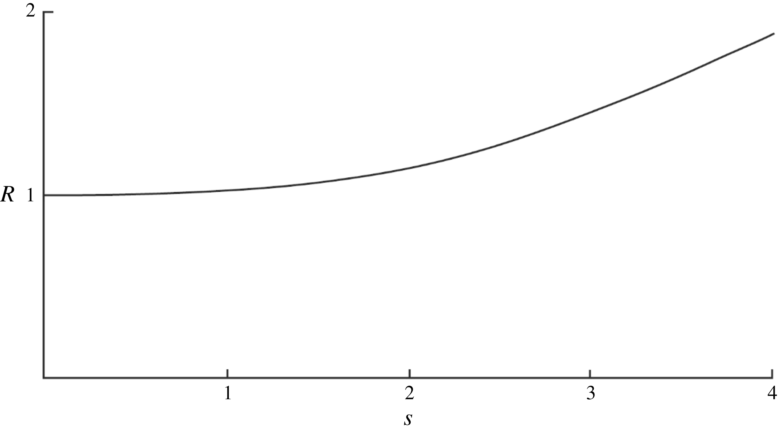
The ratio of the potential energy density to the kinetic energy density,
 $R$
, is shown in figure 2 as a function of
 $s$
when
 $F=0$
. For small
 $s$
there is equipartition of energy (
 $R\approx 1$
; Yih Reference Yih1960) but when
 $s>1$
and isopycnals are folded and dense fluid is carried over less dense as illustrated in figure 1, the potential energy begins to significantly exceed the kinetic. The potential energy is independent of
 $F$
but the kinetic energy varies with
 $F$
as in (2.10), and
 $R$
is consequently a function of
 $F$
(Gill Reference Gill1982; Thorpe & Umlauf Reference Thorpe and Umlauf2002).
The ratio of the wave potential energy density to the kinetic energy density,
 $R$
, as a function of
 $s$
when
 $F=0$
.
These contributions to the available energy will later be used to assess the relative magnitude of energy dissipated in wave breaking following overturn of isopycnals or at small Richardson number (resulting in KHI) in the exact wave solution.
The potential energy of the wave disturbance (2.8) is linearly proportional to the wave steepness,
 $s$
, or wave amplitude,
 $a$
. The gain in potential energy per unit wavelength and width in the
 $y$
-direction caused by the presence of the waves, described by (2.11), is however proportional to the vertical integral of
 $\langle \unicode[STIX]{x1D702}^{2}\rangle$
, the horizontal average of the square of the vertical displacement of density,
 $\unicode[STIX]{x1D702}$
, from its level in the mean density field,
 $\unicode[STIX]{x1D70C}=\unicode[STIX]{x1D70C}_{0}(1-N^{2}z/g)$
(Yih Reference Yih1960; Thorpe Reference Thorpe1968a
), and is therefore proportional to
 $a^{2}$
. This difference in dependency on
 $a$
is because the local flow field prior to the onset of turbulence is here represented solely by the extreme flow, either of the overturning isopycnals in the case of convective instability or of Richardson number in the case of KHI, within the wave represented by the exact wave solution, and not by some average of its spatial and temporal variation. Furthermore, the representative waves will generally be of finite amplitude, and measures derived from linear small amplitude estimates of the waves, such as the wave energy density,
 $\unicode[STIX]{x1D6FA}=\unicode[STIX]{x1D70C}_{0}a^{2}\unicode[STIX]{x1D70E}^{2}(N^{2}-f^{2})/[2(\unicode[STIX]{x1D70E}^{2}-f^{2})]$
(Thorpe Reference Thorpe2005; equation (2.20)), and the ratio of potential to kinetic energy,
 $R=[1+2(F\cot \unicode[STIX]{x1D703})^{2}]^{-1}$
(Thorpe & Umlauf Reference Thorpe and Umlauf2002) are no longer valid.
2.3 The adopted methodology
Our approach is to calculate the change in the energy per unit horizontal area during mixing at the location where the flow is represented by the finite amplitude internal wave solution, and hence to estimate the loss of energy to turbulence. For each type of breaking wave, it is supposed that when some extreme value of
 $s$
is reached mixing, with conservation of mass and momentum, sets in instantaneously over a vertical range
 $z_{1}\leqslant z\leqslant z_{2}$
, a range that depends on the type of wave breaking, convective or shear, as specified later. This leads to a mean transfer of energy into turbulence per unit horizontal area,
 $E$
(i.e. a mean transfer of energy,
 $E/(z_{2}-z_{1})$
, per unit volume in
 $z_{1}\leqslant z\leqslant z_{2}$
). It is further supposed that negligible energy is radiated from the breaking region by upward or downward propagating internal waves and that breaking events are discrete. The mean rate of dissipation of turbulent kinetic energy per unit mass in the turbulent region produced by wave breaking is therefore
 $$\begin{eqnarray}\displaystyle \unicode[STIX]{x1D700}_{m}=EN/[\unicode[STIX]{x1D70C}_{0}(z_{2}-z_{1})r], & & \displaystyle\end{eqnarray}$$
where it is supposed that the turbulence generated by the wave breaking decays in a time
 $rN^{-1}$
, where
 $r$
is a non-dimensional constant. The turbulent region increases in volume with a speed
 $c_{b}$
, and hence the rate of production of turbulent kinetic energy per unit mass by a single breaker increases at a rate
 $E\boldsymbol{c}_{b}/\unicode[STIX]{x1D70C}_{0}(z_{2}-z_{1})$
.
This approach may be compared to that adopted in studies of breaking deep-water surface waves by Pizzo & Melville (Reference Pizzo and Melville2016) and Pizzo, Deike & Melville (Reference Pizzo, Deike and Melville2016), where analysis and numerical modelling benefit from being supplemented by laboratory experiments and field observations. It is found that 95 % of the energy lost from the breaking surface waves is dissipated in the first 4 wave periods after the breaking event, little energy is radiated (rather than transmitted) from the breaking of focusing wave groups, but a robust coherent vortex is formed that lasts for more than 50 wave periods after breaking (Rapp & Melville Reference Rapp and Melville1990; Melville, Veron & White Reference Melville, Veron and White2002; Pizzo & Melville Reference Pizzo and Melville2013). The energy flux in the vortex however amounts to only 2–4 % of the dissipated energy flux in the breaking wave (Pizzo et al. Reference Pizzo, Deike and Melville2016). A note about the vortices produced by the breaking internal waves is provided in appendix G, but henceforth any quasi-steady vortices generated by breaking internal waves are neglected (or regarded as part of the turbulent motion).
2.4 The breaking parameter
 $\unicode[STIX]{x1D6EC}_{I}$

Following Phillips’ (Reference Phillips1985) use of a parameter usually denoted by
 $\unicode[STIX]{x1D6EC}$
to describe the area of breaking waves on the ocean surface we adopt an internal wave breaking parameter,
 $\unicode[STIX]{x1D6EC}_{I}$
, defined as the mean area of the fronts of breaking regions per unit volume. (This differs from Thorpe (Reference Thorpe2010b
), who describes the parameter as the area projected onto the vertical.) The mean production of turbulent kinetic energy per unit mass of the fluid by the representative breaking waves is therefore
 $$\begin{eqnarray}\displaystyle \unicode[STIX]{x1D700}_{I}=Ec_{b}\unicode[STIX]{x1D6EC}_{I}/[\unicode[STIX]{x1D70C}_{0}(z_{2}-z_{1})], & & \displaystyle\end{eqnarray}$$
with
 $c_{b}$
given by (2.4). In a steady state in which the representative wave breaking provides all the turbulence this is equal to the mean rate of dissipation of turbulent kinetic energy per unit mass, denoted by
 $\unicode[STIX]{x1D700}$
.
The parameter,
 $\unicode[STIX]{x1D6EC}_{I}$
, is yet to be established by direct observation in the ocean. The dissipation rate,
 $\unicode[STIX]{x1D700}$
, is, however, related to
 $K_{\unicode[STIX]{x1D70C}}$
, the diapycnal diffusivity of density:
 $$\begin{eqnarray}\displaystyle \unicode[STIX]{x1D700}=K_{\unicode[STIX]{x1D70C}}N^{2}/\unicode[STIX]{x1D6E4} & & \displaystyle\end{eqnarray}$$
(Osborn Reference Osborn1980), where
 $\unicode[STIX]{x1D6E4}$
is an efficiency factor. Although subject to further investigation and debate (e.g. see Arneborg (Reference Arneborg2002), Thorpe (Reference Thorpe2005), § 6.7; Chalamalla & Sarkar (Reference Chalamalla and Sarkar2015), Salehipour et al. (Reference Salehipour, Peltier and Mashayek2015)), for simplicity the commonly used value,
 $\unicode[STIX]{x1D6E4}=0.2$
, is adopted here. If
 $K_{\unicode[STIX]{x1D70C}}$
is known and
 $\unicode[STIX]{x1D700}=\unicode[STIX]{x1D700}_{I}$
, equations (2.15), (2.16) and (2.4) lead to
 $$\begin{eqnarray}\displaystyle \unicode[STIX]{x1D6EC}_{I}=K_{\unicode[STIX]{x1D70C}}m(z_{2}-z_{1})/\{[E/(\unicode[STIX]{x1D70C}_{0}N^{2})]\unicode[STIX]{x1D6E4}N\cos \unicode[STIX]{x1D703}\}. & & \displaystyle\end{eqnarray}$$
Since turbulence generated by wave breaking decays in a time
 $rN^{-1}$
, the length of the turbulent regions generated by the wave breaking is
 $$\begin{eqnarray}\displaystyle L=rN^{-1}c_{b}=rm^{-1}\cos \unicode[STIX]{x1D703}, & & \displaystyle\end{eqnarray}$$
and the fraction of the water column in which turbulence occurs is therefore
 $$\begin{eqnarray}\displaystyle Q=\unicode[STIX]{x1D6EC}_{I}L=\unicode[STIX]{x1D6EC}_{I}rm^{-1}\cos \unicode[STIX]{x1D703}. & & \displaystyle\end{eqnarray}$$
It follows from (2.14), (2.15) and (2.19) that
 $$\begin{eqnarray}\displaystyle Q=\unicode[STIX]{x1D700}_{I}/\unicode[STIX]{x1D700}_{m}, & & \displaystyle\end{eqnarray}$$
as expected, since
 $\unicode[STIX]{x1D700}_{m}$
is the dissipation rate in the active turbulent regions and
 $\unicode[STIX]{x1D700}_{I}$
is the mean dissipation over the whole fluid.
If the vertical scale,
 $H$
, of density overturns observed in the ocean is equated to the scale (
 $z_{2}-z_{1}$
) of the region mixed by convection or KHI in the breaking internal waves, it follows that a non-dimensional form of the mean transfer of energy,
 $E$
, into turbulence per unit horizontal area can be written as
 $$\begin{eqnarray}\displaystyle G\equiv E/(\unicode[STIX]{x1D70C}_{0}N^{2}H^{3})=K_{\unicode[STIX]{x1D70C}}r/(\unicode[STIX]{x1D6E4}QNH^{2}). & & \displaystyle\end{eqnarray}$$
2.5 Data used to quantify the model
Measured values of quantities appearing on the right-hand side of (2.21) are available to illustrate and to evaluate the validity of the methodology developed in following sections. At
 $28\,^{\circ }$
N,
 $155\,^{\circ }$
W, in the Pacific Ocean Gregg (Reference Gregg1980, Reference Gregg and Imberger1998) reports
 $K_{\unicode[STIX]{x1D70C}}\approx 2\times 10^{-5}~\text{m}^{2}~\text{s}^{-1}$
in mid-water depths of 800–1200 m where
 $N\approx 3.1\times 10^{-3}~\text{s}^{-1}$
. Turbulent patches are typically
 $H\approx 5$
m high. (Gregg finds some that are even larger but 5 m is chosen as a representative value.) The Coriolis parameter,
 $f$
, at
 $28\,^{\circ }$
N gives
 $F=f/N=0.022$
. Whilst the region is not recognised as a ‘hot spot’ for ocean mixing, the value of
 $K_{\unicode[STIX]{x1D70C}}$
and the corresponding value of
 $\unicode[STIX]{x1D700}$
inferred from (2.16) are typical and representative of oceanic values in the observed depth range (Waterhouse et al.
Reference Waterhouse, MacKinnon, Nash, Alford, Kunze, Simmons, Polzin, St Laurent, Sun and Pinkel2014). Gregg identifies and quantifies turbulence from zero crossings of the vertical temperature gradient, finding
 $Q$
in the range 0.07 to 0.36. An intermediate value of
 $Q$
, approximately 0.16, is derived by Gregg & Sanford (Reference Gregg and Sanford1988), at
 $34\,^{\circ }$
N
 $127\,^{\circ }$
W. They use a more precise method, recognising turbulence as being active when the rate of dissipation of turbulent kinetic energy per unit mass obtained from microstructure profiling exceeds
 $16\unicode[STIX]{x1D708}N^{2}$
, where
 $\unicode[STIX]{x1D708}$
is the molecular kinematic viscosity, i.e. when the buoyancy Reynolds number,
 $Re_{b}=\unicode[STIX]{x1D700}/\unicode[STIX]{x1D708}N^{2}>16$
. Further discussion of
 $Re_{b}$
is provided in § B.2.
Gregg’s values of
 $K_{\unicode[STIX]{x1D70C}}$
,
 $N$
,
 $F$
,
 $H$
and
 $Q$
are adopted later in comparing observations with theoretical estimates and, in particular, in finding the characteristics of internal waves that, in breaking, can support the observed mixing. Taking
 $\unicode[STIX]{x1D6E4}=0.2$
and using Gregg’s values, the relation (2.16) between
 $\unicode[STIX]{x1D700}$
and
 $K_{\unicode[STIX]{x1D70C}}$
leads to an estimate of the mean rate of dissipation of turbulent kinetic energy,
 $\unicode[STIX]{x1D700}=9.6\times 10^{-10}~\text{W}~\text{kg}^{-1}$
,
 $=\unicode[STIX]{x1D700}_{\ast }$
, say, and (2.21) becomes
 $$\begin{eqnarray}\displaystyle G\equiv E/(\unicode[STIX]{x1D70C}_{0}N^{2}H^{3})=1.29\times 10^{-3}r/Q. & & \displaystyle\end{eqnarray}$$
The broad and, because of the method by which it is obtained, uncertain range of 0.07 to 0.36 for
 $Q$
found by Gregg will be shown to provide only a weak constraint on estimated quantities related to the energy transfer by breaking waves, and Gregg and Sanford’s value,
 $Q=0.16$
(close to the mean, 0.215, of Gregg’s broad range) is therefore generally used later as a control value.
A distinction is drawn between the scale,
 $H=5$
m, characterising the size of turbulent patches, those that here are represented by internal waves breaking locally by convective instability (see figure 5, later) or by KHI (figure 8), and the r.m.s. scale of overturns within the patches, characterised by the Thorpe scale,
 $L_{T}$
, or equivalently (Dillon Reference Dillon1982) by the Ozmidov length scale,
 $L_{O}=\unicode[STIX]{x1D700}^{1/2}N^{-3/2}$
. The latter can be estimated as 0.18 m taking
 $\unicode[STIX]{x1D700}=\unicode[STIX]{x1D700}_{\ast }=9.6\times 10^{-10}~\text{W}~\text{kg}^{-1}$
and
 $N=3.1\times 10^{-3}~\text{s}^{-1}$
or as
 $0.3<L_{O}~(\text{m})<0.68$
taking
 $\unicode[STIX]{x1D700}=\unicode[STIX]{x1D700}_{I}$
using (2.20) with
 $0.07<Q<0.36$
. (For convective instability direct numerical simulation (DNS) experiments by Scotti (Reference Scotti2015), find that the Thorpe scale,
 $L_{T}$
, derived from the displacements,
 $D$
–
 $d$
, greatly exceeds
 $L_{O}$
. For KHI, the DNS model of Smyth, Moum & Caldwell (Reference Smyth, Moum and Caldwell2001), finds that
 $L_{O}$
is substantially greater that
 $L_{T}$
in the overturning billows.) Observations of the mean ratio of
 $L_{T}$
to patch size range from about 0.07 in the main thermocline of the North Atlantic (Moum Reference Moum1996) to 0.17 in Lake Banyoles, Catalonia, Spain (Planella Morato, Roget & Lozovataky Reference Planella Morato, Roget and Lozovataky2011). With
 $L_{O}=0.8L_{T}$
(Dillon Reference Dillon1982) and a patch size,
 $H$
, of 5 m, the range
 $0.3<L_{O}~(\text{m})<0.68$
gives
 $0.075<L_{T}/H<0.17$
, approximately spanning the range observed and pointing to a general consistency of the chosen values.
For brevity Gregg’s and Gregg & Sanford’s data described above are henceforth referred to by ‘GS’.
3 Convective breaking
3.1 Convective overturn
It is evident from (2.3) that in the presence of internal waves with
 $s<1$
the fluid is always statically stable, i.e.
 $\text{d}\unicode[STIX]{x1D70C}/\text{d}z<0$
. If, however,
 $s>1$
the upward vertical density gradient,
 $\text{d}\unicode[STIX]{x1D70C}/\text{d}z$
, is positive for some wave phase
 $\unicode[STIX]{x1D701}$
, implying static or, when motions set in, convective instability at some locations in the waves. As shown by the stippled regions of figure 1, when
 $s>1$
sloping statically unstable regions in which the density increases upwards are formed. Their height is
 $$\begin{eqnarray}\displaystyle h_{\ast }=2a\cos ^{-1}(1/s)/s, & & \displaystyle\end{eqnarray}$$
the vertical distance derived from (2.3) between the two levels at which
 $\text{d}\unicode[STIX]{x1D70C}/\text{d}z=0$
. Isopycnals are folded over horizontal lengths,
 $l$
, given by
 $$\begin{eqnarray}\displaystyle l/h_{\ast }=[(s^{2}-1)^{1/2}-\cos ^{-1}(1/s)]/[\tan \unicode[STIX]{x1D703}\cos ^{-1}(1/s)], & & \displaystyle\end{eqnarray}$$
that increase as
 $s$
increases and
 $\unicode[STIX]{x1D703}$
decreases. Convective instability and wave breaking follows if the Rayleigh number, Ra, of the overturning regions is sufficiently large (Thorpe Reference Thorpe1994a
). Based on GS, the Rayleigh number corresponding to the height,
 $H$
,
 $Ra=N^{2}H^{4}/\unicode[STIX]{x1D708}\unicode[STIX]{x1D705}_{T}$
, is approximately
 $1.7\times 10^{9}$
, where
 $\unicode[STIX]{x1D708}$
where is the kinematic viscosity
 ${\approx}1\times 10^{-6}~\text{m}^{2}~\text{s}^{-1}$
and
 $\unicode[STIX]{x1D705}_{T}$
is the thermal conductivity
 ${\approx}1.4\times 10^{-7}~\text{m}^{2}~\text{s}^{-1}$
. This value of Ra is well beyond that at which convective motions become turbulent at a Prandtl number appropriate to the ocean (Turner Reference Turner1973). A cautionary note about the form of wave breaking is provided in § C.2.
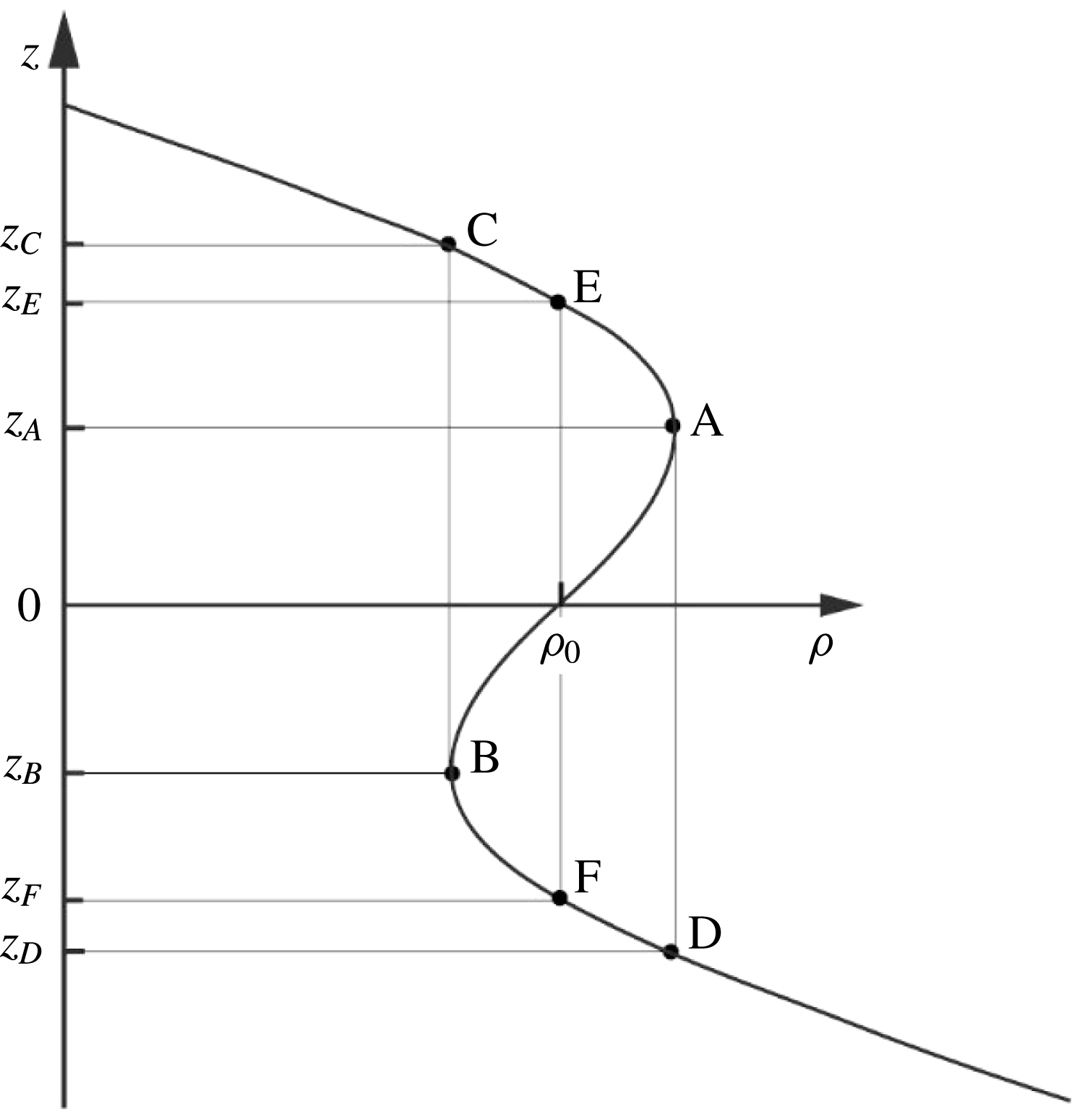
The vertical density profile at
 $x=0$
,
 $t=0$
in convectively breaking waves;
 $s>1$
. The points A and B at levels
 $z_{A}$
and
 $z_{B}$
, respectively, where the vertical density gradient is zero mark the ends of the statically unstable gradient,
 $\text{d}\unicode[STIX]{x1D70C}/\text{d}z>0$
. The density at D (or C), levels
 $z_{D}$
and
 $z_{C}$
, respectively, is equal to that at A (or B). Although the vertical density gradient is negative in the region D–B implying static stability, there is overlying fluid, B–A–C, with parts denser than fluid elements in D–B so that convection may extend downwards to D. (The layer A–C is similarly unstable having less dense fluid below it.) The whole layer, D–C, is thus potentially unstable and prone to mixing. As shown by Davies Wykes & Dalziel (Reference Davies Wykes and Dalziel2014) however, convection may result in the generation of a mixing layer spanning only the depth range F–E.

When
 $s>1$
, the vertical density profile of figure 1 at
 $x=0$
,
 $t=0$
, is as sketched in figure 3. The points A and B at
 $z=z_{A}$
and
 $z_{B}$
, respectively, where the vertical density gradient is zero, mark the ends of the statically unstable region with
 $\text{d}\unicode[STIX]{x1D70C}/\text{d}z>0$
;
 $z_{A}-z_{B}=h_{\ast }$
. The density at C (or D),
 $z=z_{C}$
(or
 $z_{D}$
) respectively, is equal to that at B (or A). The points
 $z_{C}$
and
 $z_{D}$
lie within one vertical wavelength (i.e.
 $-\unicode[STIX]{x03C0}/m<z_{D}<z_{C}<\unicode[STIX]{x03C0}/m$
) provided
 $s<4.712$
. Points E and F (
 $z_{F}<0<z_{E}$
) are where the density equals
 $\unicode[STIX]{x1D70C}_{0}$
, that at
 $z=0$
. Using (2.2) and (2.3):
 $$\begin{eqnarray}\displaystyle mz_{A}=\cos ^{-1}(1/s) & & \displaystyle\end{eqnarray}$$
(recalling
 $1/s<1$
, consistent with a wave slope exceeding unity for possible convective wave breaking),
 $mz_{C}$
is given by
 $$\begin{eqnarray}\displaystyle s\sin (mz_{C})-mz_{C}=\cos ^{-1}(1/s)-\sqrt{(s^{2}-1)}, & & \displaystyle\end{eqnarray}$$
and
 $$\begin{eqnarray}\displaystyle mz_{E}=s\sin (mz_{E}). & & \displaystyle\end{eqnarray}$$
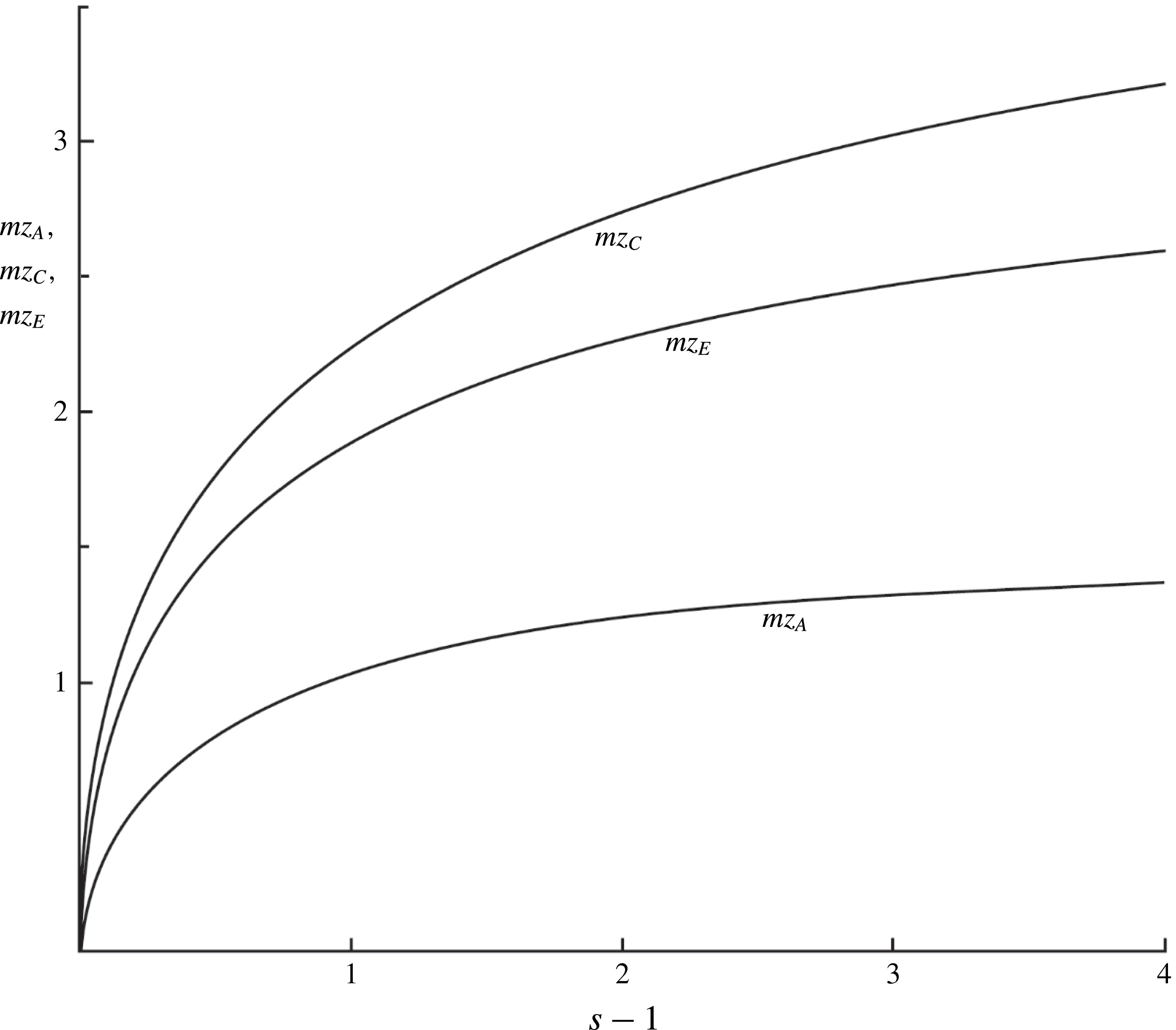
The non-dimensional heights,
 $mz_{A}$
,
 $mz_{C}$
and
 $mz_{E}$
depend only on
 $s$
and are as shown in figure 4, and
 $z_{B}=-z_{A}$
,
 $z_{D}=-z_{C}$
and
 $z_{F}=-z_{E}$
.
The variation of
 $mz_{A}$
,
 $mz_{C}$
and
 $mz_{E}$
with
 $s-1$
.

The unstable density profiles or overturns are analysed in appendix A using the method devised by van Haren & Gostiaux (Reference van Haren and Gostiaux2014).
3.2 Energy lost to turbulence
Thorpe (Reference Thorpe2010b
) adopts a model in which convection leads to mixing, homogenising the density over the height
 $h_{\ast }$
, between levels
 $z_{A}$
and
 $z_{B}$
of figure 3. The effect of mixing is to transfer potential and kinetic energy to turbulent kinetic energy. Although
 $\text{d}\unicode[STIX]{x1D70C}/\text{d}z<0$
is negative in the region D–B, implying static stability, at each level there is overlying denser fluid in B–A–C, from which convection may extend. (Similarly the layer A–C appears to be convectively unstable, having less dense fluid below it.) The whole layer, D–C, is thus potentially convectively unstable and may be involved in mixing. Choices limited by the conservation of mass and momentum are made for the (‘final’) density,
 $\unicode[STIX]{x1D70C}_{F}$
, and the velocity,
 $u_{F}$
, following mixing. The final density is supposed to be stably stratified,
 $\text{d}\unicode[STIX]{x1D70C}_{F}/\text{d}z\leqslant 0$
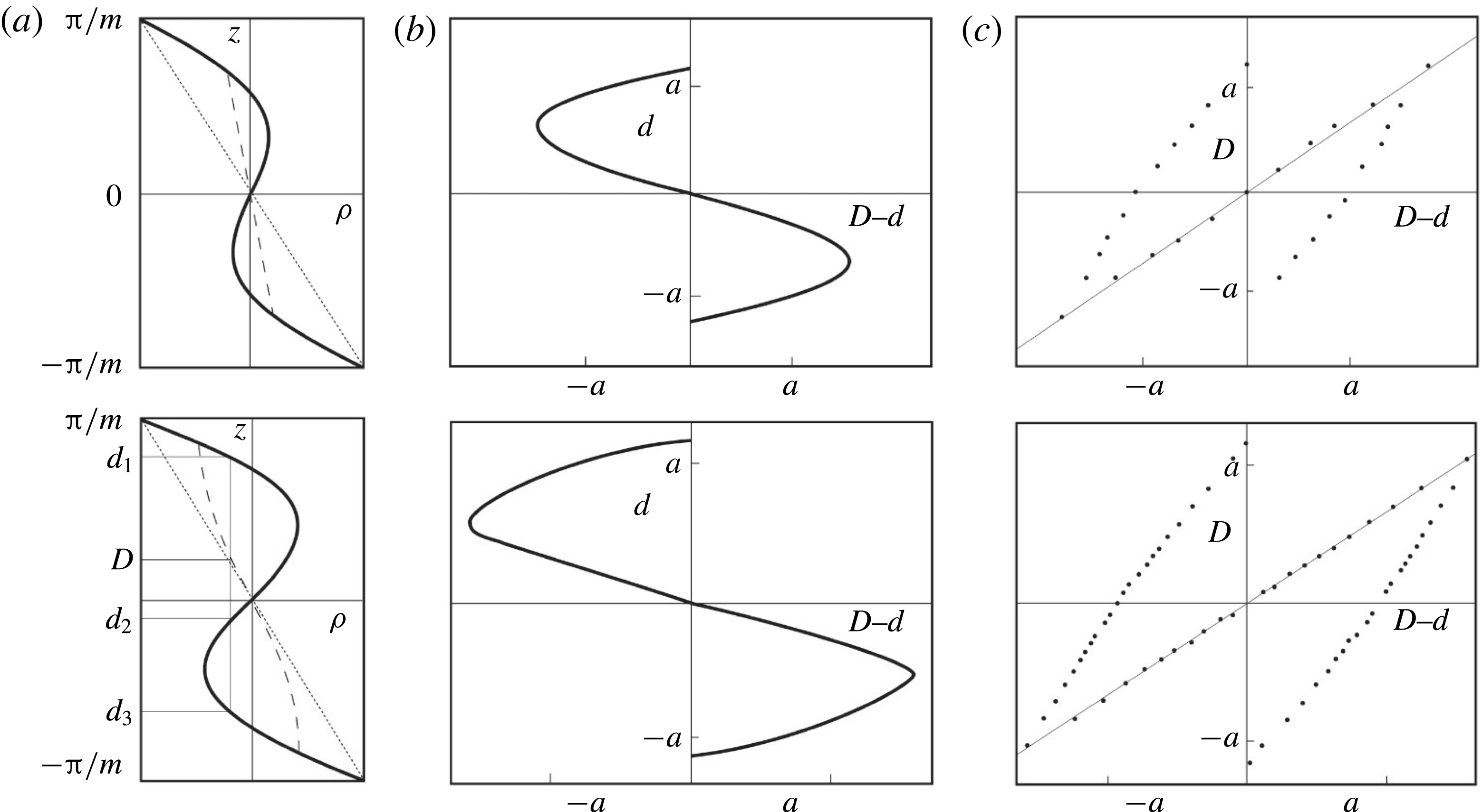
, and its range is within that of the original density; mixing cannot increase (decrease) the density to above (below) its maximum (minimum) value within the mixed region.
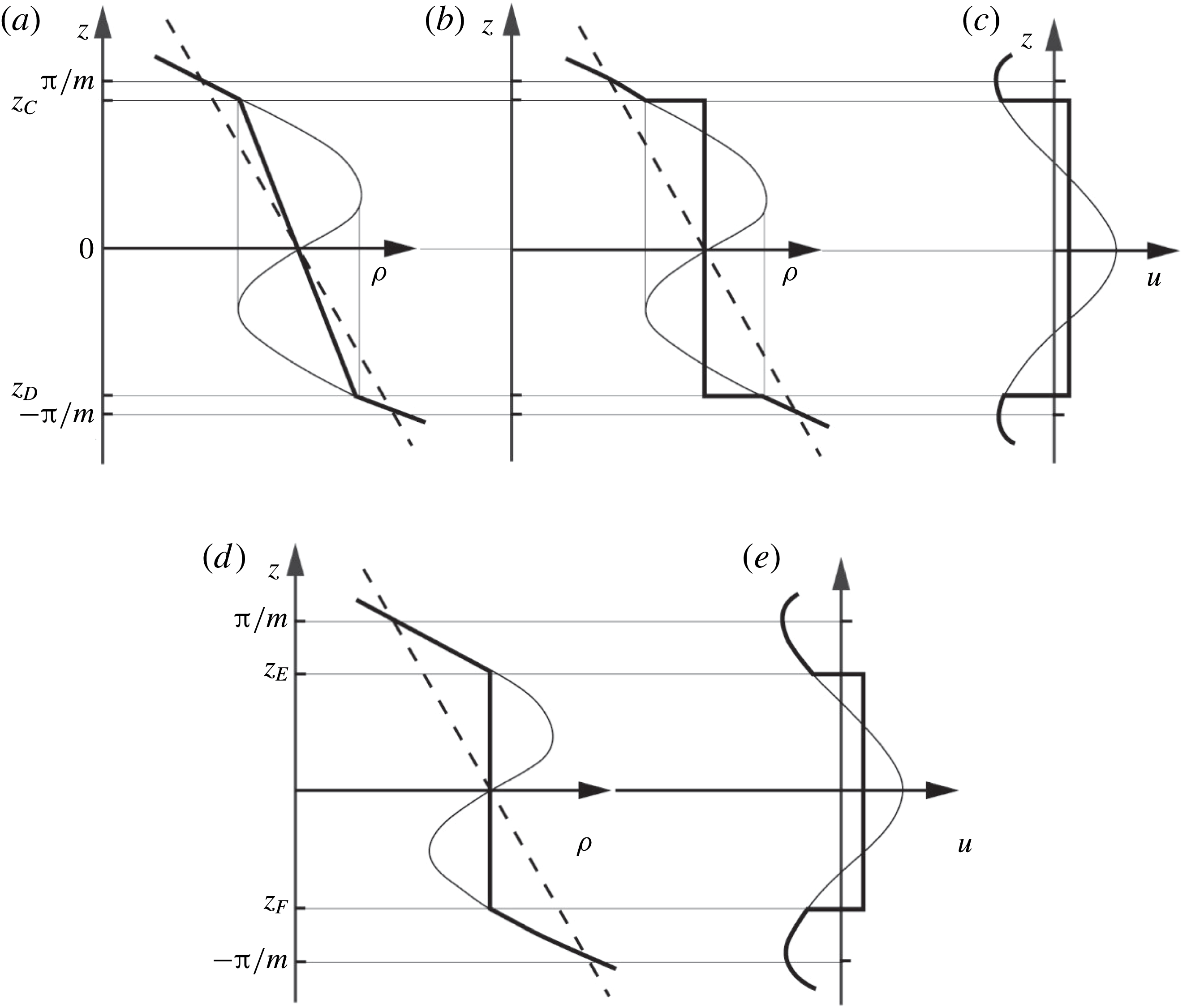
Three alternative models denoted Con1–Con3 are devised to characterise the possible density and velocity profiles after mixing and to allow some assessment of the sensitivity of the model results. The density of Con1 is shown in figure 5(a). Following convective mixing that occurs when the density gradient,
 $\text{d}\unicode[STIX]{x1D70C}/\text{d}z$
, reaches its positive maximum, a statically stable continuous linear profile of density is taken to be formed between
 $z_{D}$
and
 $z_{C}$
:
 $$\begin{eqnarray}\displaystyle \unicode[STIX]{x1D70C}_{F}=\unicode[STIX]{x1D70C}_{0}[1-(N^{2}z/gz_{C})(a\sin mz_{A}-z_{A})]. & & \displaystyle\end{eqnarray}$$
For small
 $s$
, this corresponds closely to the rearranged dashed profiles of figure 11(a) in appendix A to which (without diffusion) the elements of fluid would collapse as a consequence of convection. In Con2 the density becomes uniform with
 $\unicode[STIX]{x1D70C}_{F}=\unicode[STIX]{x1D70C}_{0}$
between levels
 $z_{C}$
and
 $z_{D}$
(figure 5
b). In both models the assumption is made that, as a result of the convective mixing, the velocity becomes uniform between levels D and C of figure 3 and equal to the mean velocity
 $\langle u\rangle =[\int u\,\text{d}z]/(z_{C}-z_{D})$
with integration from
 $z_{D}$
to
 $z_{C}$
, thus conserving momentum (figure 5
c).
A sketch showing the profiles of density,
 $\unicode[STIX]{x1D70C}$
, and
 $x$
-velocity component,
 $u$
, in convective breaking. The finer lines are the profiles of
 $\unicode[STIX]{x1D70C}$
and
 $u$
before mixing is induced by wave breaking and the thicker lines,
 $\unicode[STIX]{x1D70C}_{F}$
and
 $u_{F}$
, those after mixing. (a) Density,
 $\unicode[STIX]{x1D70C}$
and
 $\unicode[STIX]{x1D70C}_{F}$
(model Con1); (b) density,
 $\unicode[STIX]{x1D70C}$
and
 $\unicode[STIX]{x1D70C}_{F}$
(Con2); (c)
 $x$
-velocity component,
 $u$
and
 $u_{F}$
(Con1 and 2); (d) density,
 $\unicode[STIX]{x1D70C}$
and
 $\unicode[STIX]{x1D70C}_{F}$
(Con3); and (e):
 $x$
-velocity component
 $u$
and
 $u_{F}$
(Con3). Dashed lines in (a), (b) and (d) are the mean density,
 $\unicode[STIX]{x1D70C}_{0}(1-N^{2}z/g)$
.

The density,
 $\unicode[STIX]{x1D70C}_{F}$
, of the third model, Con3, is prompted by the results and analysis of laboratory experiments by Davies Wykes & Dalziel (Reference Davies Wykes and Dalziel2014) in which convection occurs across a horizontal statically unstable interface between two stably stratified fluids. The experiments reduce the statically unstable region between A and B in figure 3 to a narrow interface and do not include the effects of horizontal motion,
 $u$
. Convective mixing results in a nearly uniform layer extending between the levels equivalent to E and F of figure 3, corresponding closely, in Davies Wykes & Dalziel’s terminology, to ‘perfect mixing efficiency’. The final density and velocity profiles in Con3 are chosen similarly, as in figures 5(d) and 5(e), respectively. The energy of internal waves radiated upwards or downwards from the convective mixing region in the laboratory experiments is less than 0.2 % of the initial available potential energy and, as assumed above, is very small. In all three models rotation is disregarded by taking
 $F=0$
so that
 $v$
and
 $\unicode[STIX]{x1D703}_{b}$
are zero, the latter implying that breaking advances horizontally.
The energy lost to turbulence per unit horizontal area during the breaking process in
 $z_{D}\leqslant z\leqslant z_{C}$
in Con1 and Con2, or in
 $z_{F}\leqslant z\leqslant z_{E}$
in Con3, the net initial energy minus the final energy, is
 $$\begin{eqnarray}\displaystyle E_{c}=KE_{c}+PE_{c}, & & \displaystyle\end{eqnarray}$$
where
 $$\begin{eqnarray}\displaystyle KE_{c}=(\unicode[STIX]{x1D70C}_{0}/2)\int u^{2}\,\text{d}z-KE_{cF}, & & \displaystyle\end{eqnarray}$$
is the kinetic energy loss, with final kinetic energy,
 $KE_{cF}=(\unicode[STIX]{x1D70C}_{0}/2)\int u_{F}^{2}\,\text{d}z$
, and
 $$\begin{eqnarray}\displaystyle PE_{c}=g\int z\unicode[STIX]{x1D70C}\,\text{d}z-PE_{cF}, & & \displaystyle\end{eqnarray}$$
with
 $PE_{cF}=g\int z\unicode[STIX]{x1D70C}_{F}\,\text{d}z$
, is the potential energy loss relative to
 $z=0$
per unit horizontal area in mixing the layer, where integration is over the range,
 $z_{D}\leqslant z\leqslant z_{C}$
for Con1 and Con2 or
 $z_{F}\leqslant z\leqslant z_{E}$
for Con3,
 $u$
and
 $\unicode[STIX]{x1D70C}$
being evaluated at
 $x=t=0$
. Possible limiting (extreme) values of
 $E_{c}$
are discussed later in § B.2.
For Con1 and Con2 the vertical distance,
 $2z_{C}$
, between points D and C in figure 3 is taken to be equal to
 $H$
, the size of turbulent patches; GS. This gives
 $$\begin{eqnarray}\displaystyle m=2mz_{C}/H, & & \displaystyle\end{eqnarray}$$
with
 $mz_{C}$
given by (3.4).
The kinetic and potential energies,
 $KE_{c}$
and
 $PE_{c}$
are expressed in non-dimensional forms in terms of
 $\unicode[STIX]{x1D70C}_{0}N^{2}H^{3}$
in (B 1) and (B 2) of § B.1 and, together with
 $E_{c}/(\unicode[STIX]{x1D70C}_{0}N^{2}H^{3})$
derived using (3.7), depend only on
 $s$
and
 $\unicode[STIX]{x1D703}$
.
Using Davies Wykes & Dalziel’s (Reference Davies Wykes and Dalziel2014) results, it is shown in § C.1 that provided (
 $s-1$
) is sufficiently large or the angle,
 $\unicode[STIX]{x1D703}$
, is small, the growth time of convective instability is small in comparison to the period of time in which the density gradient in an internal wave with
 $s>1$
is negative at
 $x=z=0$
. Breaking by convective instability is then relatively instantaneous or, with respect to the growth of instability, the wave may be regarded as ‘frozen’.
The fraction of the water column that is turbulent,
 $Q$
, is given by (2.19) in terms of
 $\unicode[STIX]{x1D703}$
,
 $m$
(3.10),
 $\unicode[STIX]{x1D6EC}_{I}$
and the non-dimensional decay time constant
 $r$
(
 $=\,r_{c}$
, say). Smyth, Zavialov & Moum’s (Reference Smyth, Zavialov and Moum1997) observations of the decay time of an isolated near-surface turbulent layer gives
 $r_{c}\approx 6$
. The laboratory experiments by Davies Wykes & Dalziel (Reference Davies Wykes and Dalziel2014) find that growth ceases at a value of
 $r_{c}$
(their value
 $\unicode[STIX]{x1D70F}\approx 4$
) that decreases with
 $s$
from approximately 10.4 at
 $s=1.4$
to 4.8 at
 $s=3$
, with an approximate variation
 $$\begin{eqnarray}\displaystyle r_{c}=15.1s^{-1.06}, & & \displaystyle\end{eqnarray}$$
appropriate for Con3. (Decay of turbulence generated by convective wave breaking will generally occur at times less than half the wave period, i.e.
 $r_{c}N^{-1}<\unicode[STIX]{x03C0}\unicode[STIX]{x1D70E}^{-1}$
if
 $\unicode[STIX]{x1D703}\leqslant 32^{\circ }$
when
 $r_{c}=6$
, or if
 $\unicode[STIX]{x1D703}\leqslant 15^{\circ }$
when
 $r_{c}=12$
.)
Equation (2.17) provides a means to estimate the non-dimensional breaking parameter,
 $\unicode[STIX]{x1D6EC}_{I}H$
, with
 $z_{2}-z_{1}=2z_{C}$
,
 $=H$
, for Con1 and Con2, or
 $z_{2}-z_{1}=2z_{E}$
,
 $=H$
, for Con3. For selected values of
 $s$
and
 $\unicode[STIX]{x1D703}$
,
 $mz_{C}$
(3.4),
 $mz_{E}$
(3.5) and
 $E_{c}/(\unicode[STIX]{x1D70C}_{0}N^{2}H^{3})$
are known and the size of
 $\unicode[STIX]{x1D6EC}_{I}H$
required to support mixing can be estimated using the observed values of
 $K_{\unicode[STIX]{x1D70C}}$
,
 $N$
and
 $H$
.
3.3 Results; convective instability
For Con1 and 3 and with
 $Q$
within the range, 0.07–0.36 (GS; § 2.5), most of the energy lost to turbulence is derived from potential energy, i.e.
 $PE_{c}>KE_{c}$
, but for Con2
 $PE_{c}<KE_{c}$
, in the same range of
 $Q$
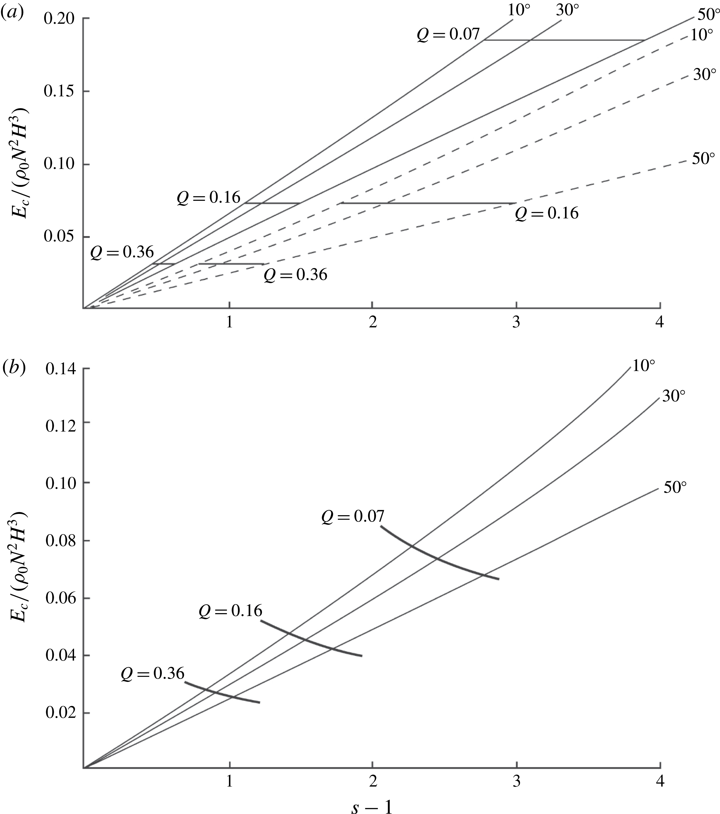
. For a given model, the non-dimensional energy transfer to turbulence,
 $E_{c}/(\unicode[STIX]{x1D70C}_{0}N^{2}H^{3})$
, is a function only of the wave characteristics,
 $s$
and
 $\unicode[STIX]{x1D703}$
, as shown in figure 6. For Con1:
 $$\begin{eqnarray}\displaystyle E_{c}/(\unicode[STIX]{x1D70C}_{0}N^{2}H^{3})=6.45(1\pm 0.016)(s-1)(\cos \unicode[STIX]{x1D703})^{0.57}\times 10^{-2}; & & \displaystyle\end{eqnarray}$$
for Con2:
 $$\begin{eqnarray}\displaystyle E_{c}/(\unicode[STIX]{x1D70C}_{0}N^{2}H^{3})=3.90(1\pm 0.015)(s-1)(\cos \unicode[STIX]{x1D703})\times 10^{-2}, & & \displaystyle\end{eqnarray}$$
and for Con3:
 $$\begin{eqnarray}\displaystyle E_{c}/(\unicode[STIX]{x1D70C}_{0}N^{2}H^{3})=3.37(1\pm 0.009)(s-1)(\cos \unicode[STIX]{x1D703})^{0.78}\times 10^{-2}, & & \displaystyle\end{eqnarray}$$
when
 $Q$
is in Gregg’s range,
 $0.07<Q<0.36$
.
The non-dimensional energy transferred to turbulence by convective breaking of waves as a function of
 $s-1$
at
 $\unicode[STIX]{x1D703}=10^{\circ }$
,
 $30^{\circ }$
and
 $50^{\circ }$
, together with (bold lines) values at
 $Q=0.07$
, 0.16 and 0.36; GS. (a) The full lines show Con1 and the dashed lines are Con2. (b) The same for Con3.

For Con1 and Con2 to match the observations of GS, the model estimates of the non-dimensional transfer of energy to turbulence must be equal to
 $G=0.0116/Q$
, given by (2.22) using
 $r=r_{c}\approx 9$
, but with an uncertainty in
 $G$
of approximately 30 % to allow for that in
 $r_{c}$
. The values of
 $G$
at
 $Q=0.07$
, 0.16 and 0.36 are indicated by the horizontal lines in figure 6(a). Breaking waves within a range of characteristics,
 $s$
and
 $\unicode[STIX]{x1D703}$
, covered by these lines can, alone, produce the observed mixing. For model Con1, values of
 $Q$
within the range, 0.07 to 0.36, are found only between
 $s=1.49$
at
 $\unicode[STIX]{x1D703}=10^{\circ }$
(at the limit
 $Q=0.36$
) and
 $s=4.91$
at
 $\unicode[STIX]{x1D703}=50^{\circ }$
(when
 $Q=0.07$
). (The latter
 $s$
exceeds 4.712 and is strictly beyond the range of model validity; § 3.1.) Higher values of
 $s$
are found for Con2; the broad range of
 $Q$
estimated by Gregg (Reference Gregg1980, Reference Gregg and Imberger1998) provides only a weak constraint on the possible range of wave characteristics,
 $s$
and
 $\unicode[STIX]{x1D703}$
, involved in wave breaking. Values of
 $s$
at Gregg & Sanford’s (Gregg & Sanford (Reference Gregg and Sanford1988)) value,
 $Q=0.16$
, are 2.15 and 2.50 for Con1 at
 $\unicode[STIX]{x1D703}=10^{\circ }$
and
 $50^{\circ }$
, respectively, and 2.77 and 4.00 for model Con2 at the same values of
 $\unicode[STIX]{x1D703}$
. Within these narrower ranges of
 $s$
, equation (3.12) for Con1, and (3.13) for Con2 with
 $G\equiv E/(\unicode[STIX]{x1D70C}_{0}N^{2}H^{3})=0.0725$
at
 $Q=0.16$
provide the values of wave steepness required for representative waves with given
 $\unicode[STIX]{x1D703}$
(or, using
 $\unicode[STIX]{x1D70E}=N\sin \unicode[STIX]{x1D703}$
, of a given wave frequency) to break and produce sufficient mixing to support the observed mixing. For example, for Con1, the required steepness is
 $$\begin{eqnarray}\displaystyle s=1+1.124(1\pm 0.016)/[1-(\unicode[STIX]{x1D70E}/N)^{2}]^{0.285}. & & \displaystyle\end{eqnarray}$$
Using (3.11) and (2.22),
 $G\equiv E_{c}/(\unicode[STIX]{x1D70C}_{0}N^{2}H^{3})=0.0185/(Qs^{1.06})$
for Con3. The values of
 $G(s)$
at
 $Q=0.07$
, 0.16 and 0.36 are indicated in figure 6(b). The curve
 $Q=0.16$
intersects the calculated non-dimensional values of
 $E_{c}/(\unicode[STIX]{x1D70C}_{0}N^{2}H^{3})$
at
 $s=2.43$
and 2.75 when
 $\unicode[STIX]{x1D703}=10^{\circ }$
and
 $50^{\circ }$
, respectively, between the respective values of Con1 and Con2.
The size of waves required to support the observed mixing can be determined: (3.10) and
 $s=am$
are used to obtain
 $a/H=s/2mz_{C}$
, and a fit,
 $$\begin{eqnarray}\displaystyle mz_{C}=2.19(s-1)^{0.375} & & \displaystyle\end{eqnarray}$$
to the curve in figure 4 relating
 $mz_{C}$
to
 $s$
when
 $0.2<(s-1)<2$
, leads to
 $$\begin{eqnarray}\displaystyle a/H=0.228s(s-1)^{-0.375}, & & \displaystyle\end{eqnarray}$$
providing an expression for the required amplitude of the representative waves. Taking the above estimates of
 $s$
and
 $\unicode[STIX]{x1D703}$
in model Con1 at
 $Q=0.16$
to be typical,
 $a/H=0.47$
at
 $s=2.15$
, the lower limit at
 $\unicode[STIX]{x1D703}=10^{\circ }$
(
 $\unicode[STIX]{x1D70E}/N=0.174$
), and
 $a/H=0.49$
at
 $s=2.50$
, the upper limit at
 $\unicode[STIX]{x1D703}=50^{\circ }$
(
 $\unicode[STIX]{x1D70E}/N=0.766$
). The corresponding vertical and horizontal wavelengths,
 $\unicode[STIX]{x1D706}_{v}$
and
 $\unicode[STIX]{x1D706}_{h}$
(or
 $2\unicode[STIX]{x03C0}m^{-1}$
and
 $\unicode[STIX]{x1D706}_{v}/\tan \unicode[STIX]{x1D703}$
, respectively) are given in non-dimensional forms
 $\unicode[STIX]{x1D706}_{v}/H$
and
 $\unicode[STIX]{x1D706}_{h}/H$
, as 1.36, 7.74 and 1.23, 1.03, respectively. Using
 $H=5$
m, the vertical wavelengths are typically 6 m, and the horizontal wavelengths lie between approximately 5 and 45 m. The speeds of the breaking region,
 $c_{b}$
, and the phase speeds,
 $c=c_{b}\sin \unicode[STIX]{x1D703}$
are typically
 $5\times 10^{-3}~\text{m}~\text{s}^{-1}$
, small relative to typical oceanic flow speeds of
 $0.1~\text{m}~\text{s}^{\text{-1}}$
(and are also relatively small for waves breaking by KHI).
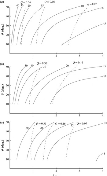
The non-dimensional breaking parameter,
 $\unicode[STIX]{x1D6EC}_{I}H$
, and contours of
 $Q$
are shown in figures 7(a) (Con1), 7(b) (Con2) and 7(c) (Con3).
 $\unicode[STIX]{x1D6EC}_{I}H$
is typically in the range of 0.05 to 0.3 (or
 $0.01<\unicode[STIX]{x1D6EC}_{I}~(\text{m}^{-1})<0.06$
if
 $H=5$
m),
 $10^{\circ }<\unicode[STIX]{x1D703}<50^{\circ }$
and when
 $Q$
is in the observed range,
 $0.07<Q<0.36$
.
Contours of constant
 $10^{2}\unicode[STIX]{x1D6EC}_{I}H$
(labelled full lines) and
 $Q$
(dashed lines) in the (
 $s-1$
,
 $\unicode[STIX]{x1D703}$
) plane for models (a) Con1; (b) Con2; (c) Con3.

The energy lost,
 $E_{c}$
, in
 $z_{D}\leqslant z\leqslant z_{C}$
for Con1 and Con2 (or
 $z_{F}\leqslant z\leqslant z_{E}$
for Con3) may be compared to that available in the same layer in the waves immediately before breaking,
 $E_{cw}$
, given by (B 3) in § B.1. The ratio
 $E_{c}/E_{cw}$
increases with
 $s$
at given
 $\unicode[STIX]{x1D703}$
but generally lies between 0.36 and 0.94 (Con1), 0.29 and 0.62 (Con2) or 0.35 and 0.58 (Con3) when
 $Q$
is in the observed GS range: to support the required mixing a substantial fraction of the localised wave energy must necessarily be dissipated and transferred to turbulence by convective overturn. The mean energy per unit mass,
 $E_{w}^{\ast }$
, at the location where breaking of individual waves is imminent, lies in the range
 $1.9\times 10^{-5}~\text{J}~\text{kg}^{-1}$
to
 $7.7\times 10^{-5}~\text{J}~\text{kg}^{-1}$
. Significantly, this is much less than the known mean energy of the internal wave field of approximately
 $1\times 10^{-3}~\text{J}~\text{kg}^{-1}$
(§ 1.1; an approximation to that in the region of GS data). It follows that even at the extreme conditions where breaking is imminent the local energy of the waves, of whatever steepness, required to produce the required mixing can be accommodated by the energy available in the oceanic internal wave field and is a relatively small energetic component of the whole field. The mean rate of dissipation of turbulent kinetic energy per unit mass in the turbulent region produced by wave breaking is, by (2.20),
 $\unicode[STIX]{x1D700}_{m}=\unicode[STIX]{x1D700}_{I}/Q$
, exceeding the overall volume mean dissipation rate,
 $\unicode[STIX]{x1D700}_{\ast }$
, as they should, for values of
 $Q$
(
 ${<}1$
) within Gregg’s range.
3.4 Summary; convective wave breaking
Three models of the mixing produced by convective wave breaking, Con1–3 shown in figure 5, are considered. They are distinguished by the degree of mixing produced in the density field and the range over which mixing occurs. Relations may be found, e.g. equation (3.15), for the steepness of waves of given frequency which represents the flow prior to mixing and which, in breaking, provide mixing sufficient to support the values of GS. Waves must be of rather small scale, both in amplitude (typically 2–3 m), wavelength (order at most a few tens of metres) and propagation speed (typically
 $5\times 10^{-3}~\text{m}~\text{s}^{-1}$
), and have a steepness of at least 1.49 (Con1 when
 $Q=0.36$
and
 $\unicode[STIX]{x1D703}=10^{\circ }$
), with values of critical steepness increasing with the wave propagation direction,
 $\unicode[STIX]{x1D703}$
. The wave breaking parameter,
 $\unicode[STIX]{x1D6EC}_{I}$
, must be of order 0.3
 $H^{-1}$
, but the limiting value also depends on
 $\unicode[STIX]{x1D703}$
(figure 7). The figure shows that, for each model, the higher the wave frequency, the greater is the wave steepness required to provide mixing at the rates required. The energy lost from waves in the breaking process,
 $E_{c}$
, is generally a substantial fraction of that locally available,
 $E_{cw}$
, in the breaking internal wave. The energy of the waves that in breaking support the mixing necessary to sustain the stratification is however considerably less than that available in the wave field. This implies that, although the required steepness of a wave breaking locally by convective instability is rather high, the wave field contains adequate energy to support the required rates of mixing and to sustain the oceanic stratification. Regions of locally high energy density, and high
 $s$
, may not, however, be located where the representative waves have the required frequencies.
But what about breaking through KHI?
4 Breaking induced by KHI
4.1 Conditions for breaking
Thorpe (Reference Thorpe1999b
) examines the conditions for the onset of KHI in an internal wave propagating in a uniformly stratified fluid, with
 $s<1$
to ensure static stability. Including rotation the disturbances to the flow given by (2.1) and (2.3) that first become unstable are directed in the
 $x$
-direction. Again limiting consideration to
 $x=t=0$
, these equations are used to determine the gradient Richardson number related to flow in the
 $x$
-direction:
 $$\begin{eqnarray}\displaystyle Ri_{x}=[(1-s\cos mz)/(s\sin mz)^{2}]/\{\cos ^{2}\unicode[STIX]{x1D703}[1+F^{2}(\cot ^{2}\unicode[STIX]{x1D703})]\}. & & \displaystyle\end{eqnarray}$$
Varying
 $z$
at given
 $s$
and
 $\unicode[STIX]{x1D703}$
, the minimum value of
 $Ri_{x}$
is
 $$\begin{eqnarray}\displaystyle Ri_{xc}=\{2\cos ^{2}\unicode[STIX]{x1D703}[1+(F\cot \unicode[STIX]{x1D703})^{2}][1-\sqrt{(1-s^{2})}]\}^{-1}. & & \displaystyle\end{eqnarray}$$
If
 $F=f/N=0$
it follows that
 $Ri_{xc}\geqslant \{\!2\cos ^{2}\unicode[STIX]{x1D703}\! )^{-1}\geqslant 1/2$
, so that in the absence of rotation the Richardson number in the wave-generated flow always exceeds 0.25 and (at least in a local quasi-steady flow approximation) the flow will be stable to small disturbances by the Miles–Howard theorem. Only if
 $F>0$
is
 $Ri_{xc}<0.25$
, making KHI possible. The height,
 $z_{0}$
, at which the Richardson number is minimum is given by
 $$\begin{eqnarray}\displaystyle mz_{0}=\cos ^{-1}\{[1-\sqrt{(1-s^{2})}]/s\}. & & \displaystyle\end{eqnarray}$$
If
 $s$
and
 $F$
are given, equation (4.2) may be solved to find
 $\unicode[STIX]{x1D703}$
, the direction of group propagation of a wave with steepness,
 $s=am$
, necessary to produce a chosen minimum Richardson number,
 $Ri_{xc}<0.25$
. If
 $F^{2}\ll 1$
as at the location of the observations by GS, but non-zero, the direction is given approximately by
 $\unicode[STIX]{x1D703}=F\sqrt{[q/(1-q)]}$
, where
 $q=2Ri_{xc}[1-\sqrt{(1-s^{2})}]~({<}1/2)$
or, when both
 $s$
and
 $F$
are small,
 $\unicode[STIX]{x1D703}\approx FsRi_{xc}^{1/2}$
. The angle,
 $\unicode[STIX]{x1D703}$
, is consequently small when
 $F=0.022$
(as in GS), implying that the breaking waves have a near-horizontal group velocity, and that (from (2.5)), the breaking internal waves must be near inertial (i.e. with
 $\unicode[STIX]{x1D70E}$
close to
 $f$
) for KHI to occur.
Measurements of turbulence in near-inertial waves by Alford & Gregg (Reference Alford and Gregg2001) in the Banda Sea suggest that their breaking is indeed initiated by KHI.
4.2 Energy lost to turbulence; the models
Assumptions are now made about the flow transition produced by KHI. To devise models, it is supposed that KH billows occur and generate turbulence at level
 $z_{0}$
where the minimum Richardson number,
 $Ri_{xc}$
, is reached in a wave with characteristics
 $\unicode[STIX]{x1D703}$
(or
 $\unicode[STIX]{x1D70E}$
) and
 $s$
. The turbulent motion results in homogenisation of fluid in a region surrounding the level
 $z_{0}$
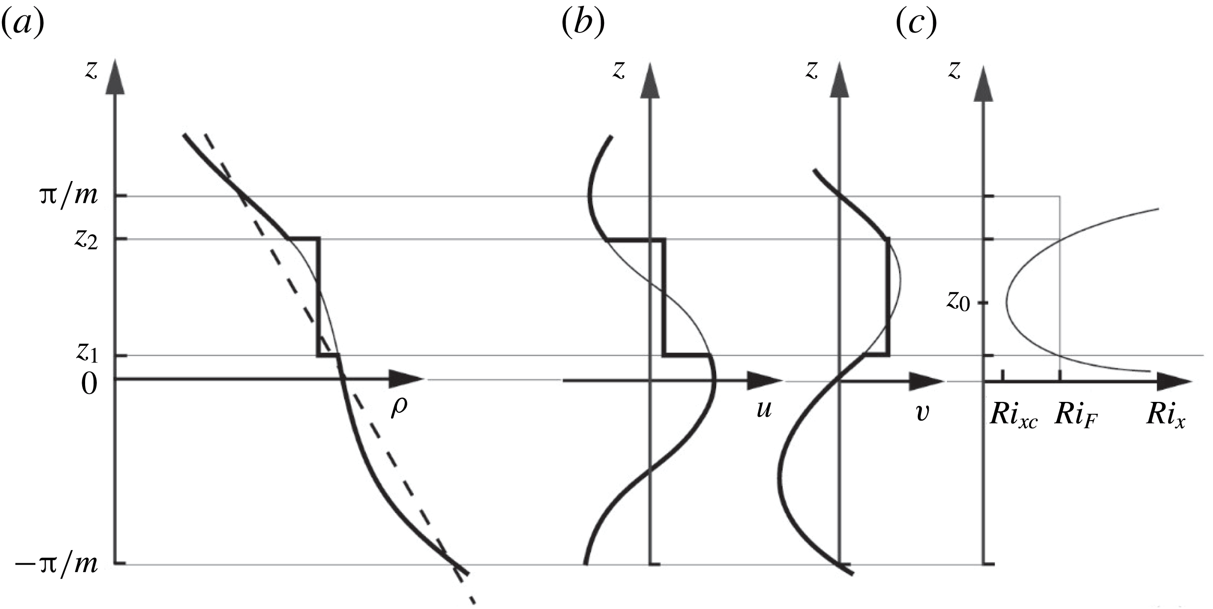
where both the density and the horizontal components of velocity become constant and equal to their mean values before breaking. The density, velocity and Richardson number profiles are sketched in figure 8. (A similar model of wave breaking is adopted by Boguski & Garrett (Reference Boguski and Garrett1993). The more natural assumption – that the final density and velocity profiles are continuous and linear rather than uniform in this region – does not provide for conservation of mass and momentum.)
A sketch showing the profiles of (a) density; (b) horizontal velocity components; and (c) gradient Richardson number,
 $Ri_{x}$
, in wave breaking through KHI. The finer lines are the profiles of
 $\unicode[STIX]{x1D70C}$
,
 $u$
and
 $v$
before mixing is induced by wave breaking, and the thicker lines,
 $\unicode[STIX]{x1D70C}_{F}$
,
 $u_{F}$
and
 $v_{F}$
, those after mixing. The minimum Richardson number,
 $Ri_{xc}$
, is at level
 $z_{0}$
. The values of
 $z$
(
 $z_{1}$
and
 $z_{2}$
) at
 $Ri_{x}=Ri_{F}$
define the vertical limits of mixing (or the size,
 $H$
, of a turbulent patch) and are within one vertical wavelength,
 $-\unicode[STIX]{x03C0}/m<z<\unicode[STIX]{x03C0}/m$
of the wave.

For how long does the wave-induced local flow at
 $x=z=0$
remain unstable to KHI? The times,
 $t_{1}$
and
 $t_{2}$
, at which the gradient Richardson number is 0.25, implying that the flow becomes potentially unstable, are given in § D.1. It is shown there that when
 $F\ll 1$
, unless
 $Ri_{xc}$
is close to 0.25, the growth times of KHI are generally much less than the period of time,
 $t_{1}$
to
 $t_{2}$
, in which instability may occur; the wave field may therefore be regarded as frozen during the period of growth of KHI. It is supposed that the flow in which turbulence is about to set in is represented by the wave model at the time at which
 $Ri_{xc}$
is reached and that mixing occurs instantaneously at this time.
The time for turbulence to collapse following KHI,
 $rN^{-1}$
, is generally much greater than the times for the growth of disturbances, and corresponds to a non-dimensional decay constant
 $r=r_{s}\approx 25$
(Thorpe Reference Thorpe1973). Provided
 $F\ll 1$
, decay will generally occur at times much less than half the wave period, i.e.
 $r_{s}N^{-1}\ll \unicode[STIX]{x03C0}\unicode[STIX]{x1D70E}^{-1}$
, for the small values of
 $\unicode[STIX]{x1D703}$
associated with near-inertial waves. Generally a local change in the direction of shear in wave propagation will not affect the decay of turbulence following KHI. (The non-dimensional times,
 $N(t_{2}-t_{1})$
, during which
 $Ri_{x}<0.25$
, are 100.6, 80.5, 62.2 and 42.1, for
 $Ri_{xc}=0.05$
, 0.1, 0.15 and 0.2, respectively, all greater than the non-dimensional time,
 $r_{s}\approx 25$
.) But, to repeat: in the models any growth of billows or turbulence developing during the time period
 $t_{1}$
to
 $t_{0}$
between the Richardson number reaching 0.25 and
 $Ri_{xc}$
are not accounted for in the estimations of mixing.
For simplicity the bounds of the mixed region are set to levels
 $z_{1}$
and
 $z_{2}$
where
 $Ri_{x}=Ri_{F}$
, with either
 $Ri_{F}=0.32$
(a value corresponding to that to which turbulence is observed to collapse following KHI in laboratory and numerical experiments as discussed in § D.2), or
 $Ri_{F}=0.25$
, the Miles–Howard stability limit. The flow after transition has a minimum gradient Richardson number
 ${\geqslant}$
0.25 and is therefore (linearly) stable by the Miles–Howard theorem. Using (4.1) and (4.2) an equation is found for the non-dimensional heights,
 $\unicode[STIX]{x1D701}=mz$
, at which
 $Ri_{x}=Ri_{F}$
in a wave in which the minimum Richardson number is
 $Ri_{xc}$
:
 $$\begin{eqnarray}\displaystyle \cos ^{2}\unicode[STIX]{x1D701}-s\unicode[STIX]{x1D712}\cos \unicode[STIX]{x1D701}+(\unicode[STIX]{x1D712}-1)=0, & & \displaystyle\end{eqnarray}$$
where
 $\unicode[STIX]{x1D712}=2[1-(1-s^{2})^{1/2}]Ri_{xc}/(s^{2}Ri_{F})$
. Equation (4.4) is a quadratic giving two roots,
 $\unicode[STIX]{x1D701}_{1}$
and
 $\unicode[STIX]{x1D701}_{2}$
, equal to
 $mz_{1}$
and
 $mz_{2}$
, respectively. It may be shown that
 $$\begin{eqnarray}\displaystyle \unicode[STIX]{x1D701}_{2}-\unicode[STIX]{x1D701}_{1}=\cos ^{-1}(2Ri_{xc}/Ri_{F}-1). & & \displaystyle\end{eqnarray}$$
In KHI there is generally a loss of kinetic energy and an increase in potential energy. The energy lost and locally transferred to turbulence per unit horizontal area at
 $x=t=0$
by wave breaking is
 $$\begin{eqnarray}\displaystyle E_{s}=KE_{s}-PE_{s}. & & \displaystyle\end{eqnarray}$$
Here
 $$\begin{eqnarray}\displaystyle KE_{s}=(\unicode[STIX]{x1D70C}_{0}/2)\int (u^{2}+v^{2})\,\text{d}z-KE_{cF}, & & \displaystyle\end{eqnarray}$$
is the kinetic energy lost, with final kinetic energy,
 $KE_{cF}$
, equal to
 $(\unicode[STIX]{x1D70C}_{0}/2)\int (u_{F}^{2}+v_{F}^{2})\,\text{d}z$
or (
 $\unicode[STIX]{x1D70C}_{0}/2$
)
 $(\langle u\rangle ^{2}+\langle v\rangle ^{2})(z_{2}-z_{1})$
if, as in the models,
 $u_{F}=\langle u\rangle$
and
 $v_{F}=\langle v\rangle$
where
 $\langle \cdots \rangle$
denotes mean values over the range,
 $z_{1}\leqslant z\leqslant z_{2}$
(or
 $\unicode[STIX]{x1D701}_{1}<\unicode[STIX]{x1D701}<\unicode[STIX]{x1D701}_{2}$
) of integration determined by the choice of
 $Ri_{F}$
. The gain in potential energy is
 $$\begin{eqnarray}\displaystyle PE_{s}=PE_{sF}-g\int z\unicode[STIX]{x1D70C}\,\text{d}z, & & \displaystyle\end{eqnarray}$$
where
 $PE_{sF}=g\int z\unicode[STIX]{x1D70C}_{F}\,\text{d}z$
is the final potential energy. As in § 3.2, choosing
 $H=z_{2}-z_{1}$
to represent the size of the mixing region gives an equation for the vertical wavenumber,
 $$\begin{eqnarray}\displaystyle m=(\unicode[STIX]{x1D701}_{2}-\unicode[STIX]{x1D701}_{1})/H; & & \displaystyle\end{eqnarray}$$
(
 $\unicode[STIX]{x1D701}_{2}-\unicode[STIX]{x1D701}_{1}$
) given by (4.5) is independent of
 $s$
, and consequently
 $m$
is also independent of
 $s$
at fixed
 $Ri_{xc}$
and
 $Ri_{F}$
. The vertical wavelength,
 $2\unicode[STIX]{x03C0}/m$
, tends to infinity as
 $Ri_{xc}$
tends to
 $Ri_{F}$
when
 $\unicode[STIX]{x1D701}_{2}-\unicode[STIX]{x1D701}_{1}$
tends to zero.
Equations for the energies non-dimensionalised by
 $\unicode[STIX]{x1D70C}_{0}N^{2}H^{3}$
are given in § E.1 in terms of
 $\unicode[STIX]{x1D701}_{1}$
and
 $\unicode[STIX]{x1D701}_{2}$
. As in § 3.2, equation (2.17) provides an equation to estimate the breaking parameter,
 $\unicode[STIX]{x1D6EC}_{I}$
, non-dimensionalised with
 $H$
:
 $$\begin{eqnarray}\displaystyle \unicode[STIX]{x1D6EC}_{I}H=[(\unicode[STIX]{x1D701}_{2}-\unicode[STIX]{x1D701}_{1})K_{\unicode[STIX]{x1D70C}}/\unicode[STIX]{x1D6E4}NH^{2}]/\{[E_{s}/(\unicode[STIX]{x1D70C}_{0}N^{2}H^{3})]\cos \unicode[STIX]{x1D703}\}. & & \displaystyle\end{eqnarray}$$
The fraction of the water column that is turbulent,
 $Q$
, is given by (2.19) in terms of
 $m$
(4.9),
 $\unicode[STIX]{x1D6EC}_{I}$
and the non-dimensional decay time constant
 $r_{s}$
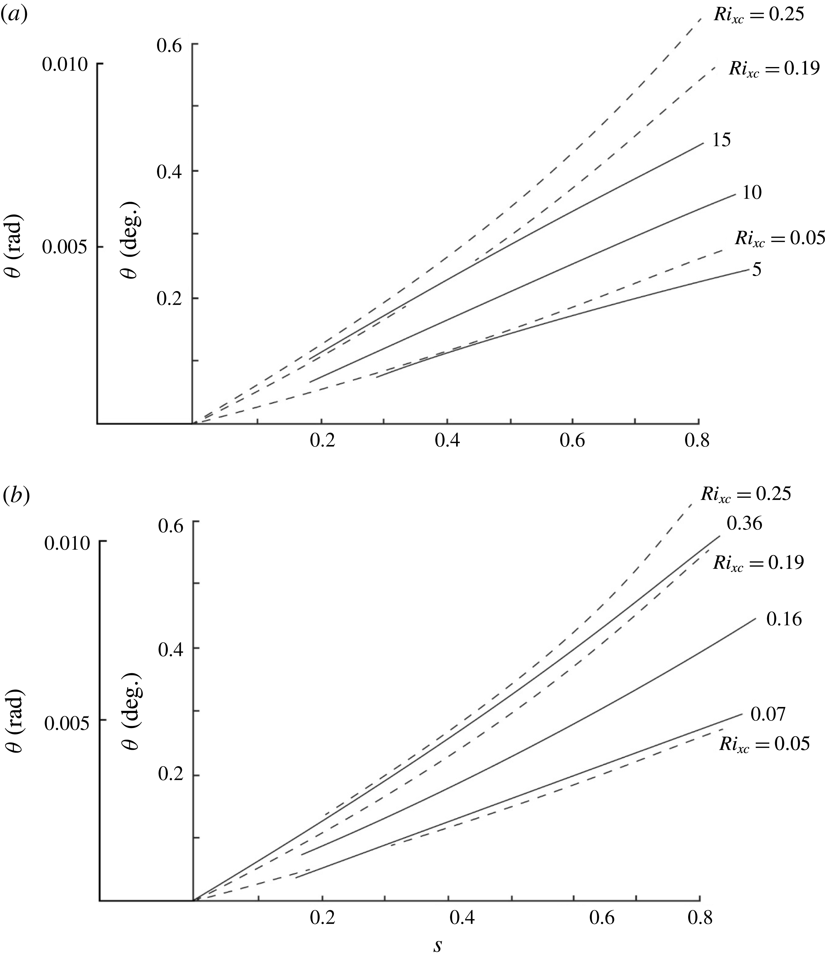
. Contours of
 $\unicode[STIX]{x1D6EC}_{I}H$
and
 $Q$
are shown in figures 10(a) and 10(b), respectively, as functions of the wave characteristics,
 $s$
and
 $\unicode[STIX]{x1D703}$
, when
 $Ri_{F}=0.32$
. (Contours of
 $\unicode[STIX]{x1D6EC}_{I}H$
and
 $Q$
when
 $Ri_{F}=1/4$
are similar to those of
 $Ri_{F}=0.32$
except close to the curve
 $Ri_{xc}=0.25$
where, from (4.5), (
 $\unicode[STIX]{x1D701}_{2}-\unicode[STIX]{x1D701}_{1}$
) tends to zero, leading to singularities in
 $KE_{s}$
given by (E 1) in § E.1.)
4.3 Results; KHI
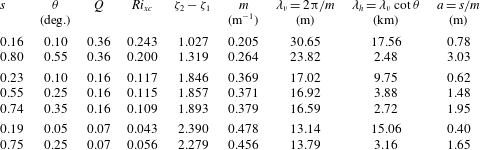
The breaking internal waves are specified by wave steepness,
 $s$
, and a frequency determined from
 $\unicode[STIX]{x1D703}$
through the dispersion relation, equation (2.5). For values of
 $Ri_{xc}$
less than approximately 0.19, equivalent values of energy-related quantities estimated with
 $Ri_{F}=0.25$
and 0.32 are of comparable magnitude and are not very sensitive to its choice. Attention is focussed on the model with
 $Ri_{F}=0.32$
. The lines
 $Q=\text{constant}$
correspond to constant values of
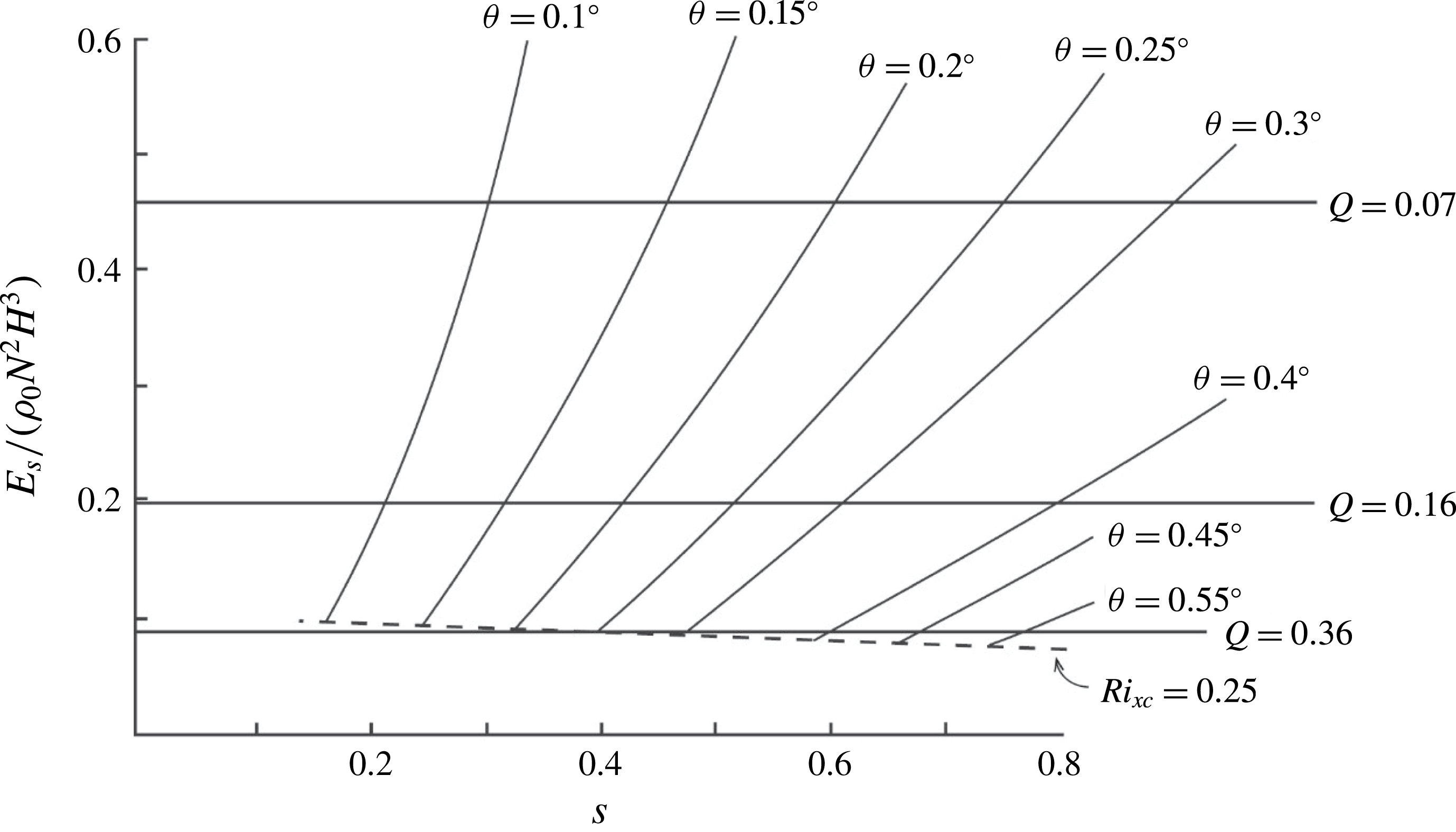
 $E_{s}/(\unicode[STIX]{x1D70C}_{0}N^{2}H^{3})$
as shown in figure 9 when
 $Ri_{F}=0.32$
. The curves of constant
 $\unicode[STIX]{x1D703}$
drawn in figure 9 are terminated at the Miles–Howard stability limit,
 $Ri_{xc}=0.25$
above which the flow is likely to be stable. Points between the lines
 $Q=0.07$
and 0.36 in this figure determine the range of characteristics of the breaking waves that can support the mixing observed by Gregg’s (Reference Gregg1980, Reference Gregg and Imberger1998) observations. For example, the observed mixing can be sustained by waves with
 $\unicode[STIX]{x1D703}=0.2^{\circ }$
(or a frequency,
 $\unicode[STIX]{x1D70E}$
, of 1.013
 $f$
using
 $F=f/N=0.022$
; GS) provided their steepness,
 $s$
, is between 0.32 (at
 $Q=0.36$
) and 0.61 (
 $Q=0.07$
) or, using (4.2), for
 $Ri_{xc}$
between 0.233 and 0.0591, respectively.
The variation of the non-dimensional energy transfer to turbulence in waves breaking through KHI with
 $Ri_{F}=0.32$
as a function of the wave steepness,
 $s$
, at set values of
 $\unicode[STIX]{x1D703}$
(deg). Values of
 $Q$
(bold lines) determined by GS and the curve
 $Ri_{xc}=0.25$
are also shown.

More generally the required wave steepness can be estimated by expressing the non-dimensionalised energy loss to turbulence,
 $E_{s}/\unicode[STIX]{x1D70C}_{0}N^{2}H^{3}$
, as a function of the wave characteristics,
 $s$
and
 $\unicode[STIX]{x1D703}$
, and of
 $F$
, given approximately by
 $$\begin{eqnarray}\displaystyle E_{s}/\unicode[STIX]{x1D70C}_{0}N^{2}H^{3}=2.61(1\pm 0.034)\times 10^{-2}(sF/\unicode[STIX]{x1D703})^{2.11}, & & \displaystyle\end{eqnarray}$$
where
 $\unicode[STIX]{x1D703}$
is measured in radians. Relations between the wave frequency and its steepness, those required for dissipation through breaking to be consistent with GS, are now obtained using (4.11) and (2.22) with
 $E=E_{s}$
and
 $r=r_{s}$
. For example, when
 $Q=0.16$
, equation (2.22) gives
 $E_{s}/\unicode[STIX]{x1D70C}_{0}N^{2}H^{3}=0.202$
, and with this value (4.11) leads
 $s=2.64(1\pm 0.041)(\unicode[STIX]{x1D703}/F)$
. Using (2.5) at
 $\unicode[STIX]{x1D70E}=f+$
the required wave steepness is
 $$\begin{eqnarray}\displaystyle s=3.73(1\pm 0.04)(\unicode[STIX]{x1D70E}/f-1)^{1/2}, & & \displaystyle\end{eqnarray}$$
increasing as
 $\unicode[STIX]{x1D70E}$
increases. When
 $\unicode[STIX]{x1D703}\ll F$
this corresponds approximately to
 $Ri_{xc}=0.14$
; a minimum Richardson number of this size is sufficient to provide mixing at the rate required to sustain the observed stratification provided
 $Q=0.16$
.
Most of the kinetic energy lost in breaking,
 $KE_{s}$
, is transferred to turbulence; only a relatively small proportion ranging from approximately 10 %–37 % contributes to an increase in potential energy. For
 $Ri_{F}=0.32$
the efficiency of wave breaking, defined here as
 $PE_{s}/KE_{s}$
, is approximately given by
 $$\begin{eqnarray}\displaystyle PE_{s}/KE_{s}=1.88(1\pm 0.011)(Ri_{xc}+0.016), & & \displaystyle\end{eqnarray}$$
increasing as
 $Ri_{xc}$
increases from approximately 0.12 at
 $Ri_{xc}\approx 0.05$
to 0.4 at
 $Ri_{xc}\approx 0.2$
.
 $KE_{s}/KE_{sw}$
is the ratio of wave kinetic energy lost to turbulence,
 $KE_{s}$
, to the kinetic energy available in the breaking wave,
 $KE_{sw}$
, for which an equation is given by (E 3) in § E.1. Generally less than 40 % of the kinetic energy initially available in the internal waves representing the flow is transferred to turbulence or to the increase of potential energy.
The magnitude of the non-dimensional wave breaking parameter,
 $\unicode[STIX]{x1D6EC}_{I}H$
, is shown in figure 10(a). The values of
 $\unicode[STIX]{x1D6EC}_{I}$
required to support turbulent dissipation at the rate
 $\unicode[STIX]{x1D700}_{\ast }=9.6\times 10^{-10}~\text{W}~\text{kg}^{-1}$
inferred by GS are typically of order
 $(5{-}15)\times 10^{-3}H^{-1}$
.
 $Q$
, shown in figure 10(b), exceeds the lower bound, 0.07, and spans most of the observed range, 0.07 to 0.36, over some range of
 $\unicode[STIX]{x1D703}$
and with
 $0.1<s<0.8$
when, approximately,
 $0.05\leqslant Ri_{xc}<0.19$
. When
 $Ri_{xc}<0.05$
the estimated values of
 $Q$
are lower than the observed; the predicted mixing is then more intense than observed. The curve
 $Q=0.16$
corresponds to (4.12) when related to
 $\unicode[STIX]{x1D703}$
by (2.5).
Contours of (a)
 $10^{3}\unicode[STIX]{x1D6EC}_{I}H$
, and (b)
 $Q$
in the (
 $s$
,
 $\unicode[STIX]{x1D703}$
) plane for waves breaking through KHI with
 $Ri_{F}=0.32$
. The curves
 $Ri_{xc}=0.25$
, 0.19 and 0.05 are shown by the dashed lines.

As in the case of convective instability described in § 3.3, the rates of dissipation of turbulent kinetic energy per unit mass in the breaking region,
 $\unicode[STIX]{x1D700}_{m}$
, exceed the mean rate,
 $\unicode[STIX]{x1D700}_{\ast }$
. The mean energy of the waves per unit mass at the point of their breaking is
 $E_{w}^{\ast }$
given by (2.13). Excluding the values affected by the limit at
 $Ri_{F}=0.25$
and those when
 $Q$
is outside the range 0.07–0.36, the values of
 $E_{w}^{\ast }$
range from
 $2.48\times 10^{-4}~\text{J}~\text{kg}^{-1}$
to
 $6.16\times 10^{-4}~\text{J}~\text{kg}^{-1}$
. This is a substantial fraction of the estimated total mean energy, approximately
 $1\times 10^{-3}~\text{J}~\text{kg}^{-1}$
, of the oceanic internal wave field.
A selection of the wave characteristics contributing to the generation of turbulence spanning a range of values of
 $Q$
and determined from figure 10(b) are listed in table 1. The non-dimensional wave amplitude,
 $a/H$
, is equal to
 $s/(\unicode[STIX]{x1D701}_{2}-\unicode[STIX]{x1D701}_{1})$
, with
 $\unicode[STIX]{x1D701}_{2}-\unicode[STIX]{x1D701}_{1}$
given by (4.5). With
 $H=5$
m, wave amplitudes are generally 0.4–3 m, and vertical and horizontal wavelengths 13–30 m and 2–18 km, respectively.
Characteristic measures of representative waves breaking by KHI with
 $Ri_{F}=0.32$
and leading to the mixing required to support the observed ocean stratification: the wave steepness,
 $s$
, and direction,
 $\unicode[STIX]{x1D703}$
, for values of the fractional volume of turbulence,
 $Q$
, spanning Gregg’s range, together with the gradient Richardson number,
 $Ri_{xc}$
, the non-dimensional vertical range of mixing after breaking,
 $\unicode[STIX]{x1D701}_{2}-\unicode[STIX]{x1D701}_{1}$
, the vertical wavenumber,
 $m$
, and wavelength,
 $\unicode[STIX]{x1D706}_{v}=2\unicode[STIX]{x03C0}/m$
, the horizontal wavelength,
 $\unicode[STIX]{x1D706}_{h}=\unicode[STIX]{x1D706}_{v}\cot \unicode[STIX]{x1D703}$
, and the wave amplitude,
 $a=s/m$
.
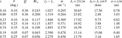
The (unlikely) case in which KHI produces no change in the density profile and
 $E_{s}$
is consequently maximised is considered in § E.2. Smaller values of
 $s$
are then required for the resulting turbulence to sustain the mixing observed by GS.
4.4 Summary; wave breaking by KHI
In local regions where they represent breaking by KHI the internal waves must be near inertial. Two model representations of breaking are examined, those in which Richardson numbers,
 $Ri_{F}$
, after mixing tends to either 0.32 or 0.25. These prove to produce similar estimates of the non-dimensional energy transfer to turbulence provided mixing occurs when the gradient Richardson number,
 $Ri_{xc}$
, is less than approximately 0.19. For simplicity attention is focused on
 $Ri_{F}=0.32$
. Most of the kinetic energy lost in breaking,
 $KE_{s}$
, is transferred to turbulence, a relatively small proportion contributing to an increase in potential energy,
 $PE_{s}$
. When turbulence sets in with
 $Ri_{x}<0.05$
mixing results in relatively large transports of energy to turbulence,
 $E_{s}$
, and the fraction of fluid that must be turbulent,
 $Q$
, to lead to the observed diffusivity,
 $K_{\unicode[STIX]{x1D70C}}$
, is less than the smallest observed, i.e. 0.07. To produce mixing consistent with GS, the amplitudes of the breaking waves must be of order 3 m, and their vertical and horizontal wavelengths of order 30 m to 18 km, respectively, although the horizontal wavelength of the wave preceding turbulence is unlikely to be representative of the size of a local turbulent patch. The values of
 $\unicode[STIX]{x1D6EC}_{I}$
needed to sustain mixing at the rates required are typically of order
 $(5{-}15)\times 10^{-3}H^{-1}$
. The internal wave energy per unit mass,
 $E_{w}^{\ast }$
, required to sustain mixing at the rate observed is generally a substantial fraction of the
 $1\times 10^{-3}~\text{J}~\text{kg}^{-1}$
estimated to be available in the total internal wave field.
5 Relaxation of the assumption that breaking waves are all of the same
$s$
and
$\unicode[STIX]{x1D70E}$


For simplicity, it was supposed in § 2.1 that the internal waves selected to represent breaking in the regions where turbulence occurs are of a single steepness,
 $s$
, and frequency,
 $\unicode[STIX]{x1D70E}$
(or, by (2.5), a single direction,
 $\unicode[STIX]{x1D703}$
). In reality it is likely that the mixing events differ substantially from one another and are better modelled by breaking internal waves with a range of steepness,
 $s$
, and frequencies,
 $\unicode[STIX]{x1D70E}$
. Suppose that
 $q(s,\unicode[STIX]{x1D703})$
is the fractional volume of the regions in which the flow, about to become turbulent, is represented by waves in the ranges of steepness,
 $s$
to
 $s+\text{d}s$
, and of directions,
 $\unicode[STIX]{x1D703}$
to
 $\unicode[STIX]{x1D703}+\text{d}\unicode[STIX]{x1D703}$
. The net volume fraction of turbulent fluid is
 $$\begin{eqnarray}\displaystyle Q=\iint q\,\text{d}s\,\text{d}\unicode[STIX]{x1D703}, & & \displaystyle\end{eqnarray}$$
where the integration is over a range of
 $s$
and
 $\unicode[STIX]{x1D703}$
determined by the waves. The vertical distance over which the representative breaking waves cause mixing is now taken to be a function of
 $s$
and
 $\unicode[STIX]{x1D703}$
:
 $h(s,\unicode[STIX]{x1D703})$
. The mean of
 $h(s,\unicode[STIX]{x1D703})$
is set equal to the observed patch scale,
 $H$
:
 $$\begin{eqnarray}\displaystyle H=\iint h\,\text{d}s\,\text{d}\unicode[STIX]{x1D703}\left/\iint \text{d}s\,\text{d}\unicode[STIX]{x1D703}.\right. & & \displaystyle\end{eqnarray}$$
The mean transfer of energy into turbulence per unit horizontal area within the regions is denoted as
 $E(s,\unicode[STIX]{x1D703})$
. To find the expressions for the energy lost in breaking from waves with characteristics
 $s$
and
 $\unicode[STIX]{x1D703}$
, earlier formulae for non-dimensional
 $E$
are revised by writing
 $h$
for
 $H$
. Following (2.14), (2.20) and (2.16), the mean rate of dissipation of turbulent kinetic energy per unit mass can be written
 $$\begin{eqnarray}\displaystyle \unicode[STIX]{x1D700}=\iint [q(E/\unicode[STIX]{x1D70C}_{0}N^{2}h^{3})N^{3}h^{3}/(z_{2}-z_{1})r]\,\text{d}s\,\text{d}\unicode[STIX]{x1D703},=K_{\unicode[STIX]{x1D70C}}N^{2}/\unicode[STIX]{x1D6E4}, & & \displaystyle\end{eqnarray}$$
which is estimated from the GS observations as
 $\unicode[STIX]{x1D700}_{\ast }=9.6\times 10^{-10}~\text{W}~\text{kg}^{-1}$
. The non-dimensional energy,
 $E/\unicode[STIX]{x1D70C}_{0}N^{2}h^{3}$
, can be expressed in terms of
 $s$
and
 $\unicode[STIX]{x1D703}$
as in (3.12)–(3.14) and (4.11). The vertical distance, (
 $z_{2}-z_{1}$
), is equal to
 $h$
.
An extension of (2.17) may be used to determine
 $\unicode[STIX]{x1D706}(s,\unicode[STIX]{x1D703})$
, the area per unit volume of the fronts of breaking regions produced by waves of steepness between
 $s$
and
 $s+\text{d}s$
and directions between
 $\unicode[STIX]{x1D703}$
and
 $\unicode[STIX]{x1D703}+\text{d}\unicode[STIX]{x1D703}$
. The mean area per unit volume gives the overall breaking parameter,
 $\unicode[STIX]{x1D6EC}_{I}$
.
In the absence of further information or observations, ad hoc equations are selected in appendix F to represent
 $q$
and
 $h$
in terms of
 $s$
and
 $\unicode[STIX]{x1D703}$
.
6 Discussion
6.1 Energy transfer
Turbulence in the ocean is patchy and intermittent. To examine the role of internal waves in producing turbulence exact solutions of the equations of motion, solutions that represent internal waves in which instability, i.e. wave breaking, is imminent, are selected to represent the velocity and density fields in the local regions where turbulence and mixing are about to develop. The instability of the waves results in mixing over an extent
 $z_{2}-z_{1}=H$
. It is initially (§§ 3 and 4) supposed that the breaking internal waves have identical steepness,
 $s$
, and direction,
 $\unicode[STIX]{x1D703}$
(or frequency,
 $\unicode[STIX]{x1D70E}$
). Values of
 $s$
and
 $\unicode[STIX]{x1D703}$
are found that best conform to the observed (GS) turbulence.
Two processes known to be involved in the instability of finite amplitude internal waves are taken to represent to the onset of turbulence. The first, convective instability, discussed in § 3, occurs only when the steepness,
 $s$
, of a wave exceeds unity. It is assumed that mixing occurs over the vertical extent of all or part of a gravitationally unstable region defined in figure 5 for three different models, Con1–3. The sum of the potential and kinetic energies lost in the transition quantifies the energy supplied to turbulence and dissipated. The major source of turbulent energy depends on the model; a loss in potential energy dominates the transfer to turbulence in Con1 and 3 but kinetic energy dominates in Con2. The non-dimensional energy dissipated by waves of steepness,
 $s$
, with direction,
 $\unicode[STIX]{x1D703}$
, is summarised in figure 6 and by (3.12)–(3.14).
The second process leading to wave breaking is KHI, § 4. This is most likely to occur in near-inertial internal waves when the local gradient Richardson number is less than 0.25. It is supposed that mixing extends to levels,
 $z_{1}$
and
 $z_{2}$
, at which the gradient Richardson number,
 $Ri_{F}$
, is equal either to 0.32 or 0.25 and results in a layer of uniform density and velocity (figure 8). Most of the kinetic energy lost in breaking is transferred to turbulence, a relatively small fraction providing an increase in the potential energy of the mean density field. The non-dimensional energy dissipated by waves of steepness,
 $s$
, with direction,
 $\unicode[STIX]{x1D703}$
, is summarised in figure 9 and by (4.11). A third process possibly leading to wave breaking, Holmboe instability (Smyth & Winters Reference Smyth and Winters2003; Salehipour, Caulfield & Peltier Reference Salehipour, Caulfield and Peltier2016) is not considered here because the relation, if any, of this instability to internal waves is yet to be firmly established.
Data obtained by Gregg (Reference Gregg1980, Reference Gregg and Imberger1998) and Gregg & Sanford (Reference Gregg and Sanford1988) are used to determine whether the energy estimated in the models to be transferred to turbulence by internal wave breaking, and then dissipated, can account for the observed overall dissipation rate. A key measure of the combined data,
 $G$
, is provided by (2.21); it sets the required energy loss. The parameter,
 $Q$
, the fractional volume of the turbulence, is related to the internal wave breaking parameter,
 $\unicode[STIX]{x1D6EC}_{I}$
, defined as the mean area of the fronts of breaking regions per unit volume.
Summary of the typical values required of the internal waves locally representing the conditions at the onset of breaking sufficient to support mixing characterised by observations GS when
 $Q=0.16$
.
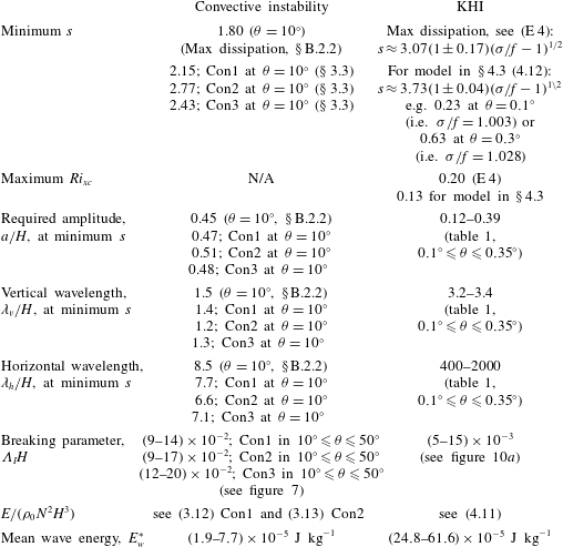
Table 2 lists parameters that characterise the waves which, in breaking, are sufficient to support the observed mixing, GS, supposing that
 $Q=0.16$
. The table provides a comparison of the effects of convective instability with
 $s$
of at least 1.8 and of KHI in near-inertial waves with
 $s<1$
but increasing as
 $\unicode[STIX]{x1D70E}/f$
increases. The smallest wave amplitude required for convective instability in the models is similar, at least 0.45H. Generally smaller amplitudes, but increasing with
 $\unicode[STIX]{x1D70E}/f$
, are required for KHI. The vertical wavelengths of the waves supporting mixing by KHI are notably greater than for convective instability but in each case they are within the range generally known as contributing to ‘oceanic fine structure’. The near-inertial breaking waves supporting KH mixing are substantially greater in horizontal wavelength than those breaking by convective instability. For convective instability to provide sufficient dissipation the breaking parameter,
 $\unicode[STIX]{x1D6EC}_{I}$
, must be of order
 $20\times 10^{-2}H^{-1}$
while for KHI the values of
 $\unicode[STIX]{x1D6EC}_{I}$
required are substantially smaller, in the range
 $(5{-}15)\times 10^{-3}H^{-1}$
. For both wave breaking by convective instability or by KHI, the energy required of the waves within the local regions in which turbulence is imminent,
 $E_{w}^{\ast }$
, is less than the
 $1\times 10^{-3}~\text{J}~\text{kg}^{-1}$
estimated to be available in the internal wave field, but a significantly larger proportion is required for KHI. Although the near-inertial waves generally contain more energy than those of higher frequency (Munk Reference Munk, Warren and Wunsch1981), it is unlikely that the extreme conditions in the local flow regions where breaking is approached are represented by waves in the mean wave spectrum. It is consequently not possible at present to determine whether the mixing resulting from convective instability or shear dominates the generation of turbulence or to test Garrett & Munk’s (Reference Garrett and Munk1972) conclusion that, except at great depths, shear instability is very much more likely to cause waves to break than convective overturning.
The requirement that all internal waves representing conditions at the onset of turbulence have the same
 $s$
or
 $\unicode[STIX]{x1D703}$
(or
 $\unicode[STIX]{x1D70E}$
) is relaxed in § 5 but at the cost of introducing yet unobserved and unmeasured distributions of the volume fraction,
 $q(s,\unicode[STIX]{x1D703})$
and the vertical scale,
 $h(s,\unicode[STIX]{x1D703})$
, of breakers. Possible choices of the distributions are made in appendix F and, for some plausible choices, succeed in providing estimates that accord with GS. A combination of breaking by convective instability and KHI remains to be considered.
6.2 Sensitivity
The selections of
 $\unicode[STIX]{x1D70C}_{F}$
and
 $u_{F}$
control the transfer of energy from the waves to turbulence. In the case of convective instability, upper and lower bounds for energy transfer,
 $E_{c}$
, and the consequent required values of wave steepness,
 $s$
, are established in § B.2. When
 $\unicode[STIX]{x1D70C}_{F}$
and
 $u_{F}$
are changed from those in figure 5 so that
 $E_{c}$
is reduced by a factor,
 $\unicode[STIX]{x1D702}$
, then from (3.12)–(3.14) (or figure 6) the values of (
 $s-1$
) required for the supply of turbulent energy at the rates in accord with GS are increased by a factor
 $\unicode[STIX]{x1D702}^{-1}$
, e.g. if
 $\unicode[STIX]{x1D702}=0.5$
the minimum value of
 $s$
in Con1 at
 $Q=0.16$
increases from 2.15 to 3.3 when
 $\unicode[STIX]{x1D703}=10^{\circ }$
, or from 2.5 to 4.0 when
 $\unicode[STIX]{x1D703}=50^{\circ }$
. The corresponding changes in
 $\unicode[STIX]{x1D6EC}_{I}H$
are increased from 0.08 to 0.11 when
 $\unicode[STIX]{x1D703}=10^{\circ }$
and from 0.14 to 0.18 when
 $\unicode[STIX]{x1D703}=50^{\circ }$
. Upper limits for dissipation by KHI and lower limits for
 $s$
are determined in § E.2 and, when
 $Q=0.16$
, the lower limits are summarised in table 2. The conclusions are sensitive to the choices of
 $\unicode[STIX]{x1D70C}_{F}$
and
 $u_{F}$
following the collapse of turbulence produced by wave breaking.
Results are also sensitive to
 $H$
. In the case of convective instability (§ 3), since
 $G$
is proportional to
 $H^{-2}$
and
 $E_{c}/\unicode[STIX]{x1D70C}_{0}N^{2}H^{3}$
is proportional to (
 $s-1$
), values of (
 $s-1$
) at given
 $Q$
in figure 6 are increased from those at
 $H=5$
m by a factor
 $(5m/H(m))^{2}$
; e.g. for there to be sufficient energy lost in wave breaking there must be an increase in
 $s$
from 2.15 to 2.76 at
 $Q=0.16$
and
 $\unicode[STIX]{x1D703}=10^{\circ }$
in Con1 as
 $H$
decreases from 5 to 4 m. At
 $H=4$
m (3.15) becomes
 $$\begin{eqnarray}\displaystyle s=1+1.77(1\pm 0.016)/[1-(\unicode[STIX]{x1D70E}/N)^{2}]^{0.285}. & & \displaystyle\end{eqnarray}$$
There is a consequent corresponding increase in
 $a/H$
(0.47–0.51) and a reduction of
 $a$
(2.4–2.0 m) and of
 $\unicode[STIX]{x1D706}_{v}$
(6.8 to 4.6 m) with a similar reduction in
 $\unicode[STIX]{x1D706}_{h}=\unicode[STIX]{x1D706}_{v}/\tan \unicode[STIX]{x1D703}$
. For KHI (§ 4), equation (4.12) becomes
 $$\begin{eqnarray}\displaystyle s=4.60(1\pm 0.04)(\unicode[STIX]{x1D70E}/f-1)^{1/2}, & & \displaystyle\end{eqnarray}$$
when
 $H=4$
m, i.e. an increase in the wave slope needed to provide the required dissipation at a given wave frequency of approximately 23 %. The corresponding
 $Ri_{xc}$
is reduced from approximately 0.14 to 0.094.
6.3 Requirements for further study
The relaxation in § 5 of the assumption that all the breaking regions are represented by waves of the same
 $s$
and
 $\unicode[STIX]{x1D703}$
exposes the requirement to obtain further information about the distributions of the volume fraction,
 $q$
, and the vertical scale,
 $h$
, of turbulent patches, and the slope of isopycnals as turbulence begins. The relation between internal waves and turbulence requires further study, in particular an investigation of the cause (convective instability or KHI) and consequences of wave breaking, and the quantification of
 $\unicode[STIX]{x1D6EC}_{I}$
and
 $\unicode[STIX]{x1D706}(s,\unicode[STIX]{x1D703})$
and of the characteristic profiles,
 $\unicode[STIX]{x1D70C}_{F}$
and
 $u_{F}$
, remaining after waves have broken. If breaking is associated with internal waves groups, it is evident that the (poorly understood) processes through which groups are formed will affect the dissipation of energy in the ocean. A major observational problem in assessing the role of groups is that they have a small propagation speed in comparison with the background velocity typical of the ocean and are consequently difficult to track and so to be identified using conventional instruments. Thorpe (Reference Thorpe2010b
) suggests how the required observations could be obtained.
The effect that breaking, or residual weakly turbulent regions, has on subsequent wave breaking is unknown. The generation of vortices by breaking internal waves has been disregarded in assessing the transfer of energy to turbulence (§ 2.1) or, at least, any such vortices are accounted for as part of the turbulent motion. It is likely that stacks of weak dipole vortices will be generated by wave breaking (appendix G) and that these contribute to the smaller scales of vortical mode in the ocean (Müller (Reference Müller1984); later references are given by Pinkel (Reference Pinkel2014), and by Kunze & Sundermeyer (Reference Kunze and Sundermeyer2015)). It may be postulated that the remnants of mixing events caused by KHI occur as patches of fluid with
 $Ri\approx 0.32$
and with organised vertical components of vorticity that diffuse or are subsequently strained by the ambient shear or by the arrival of new internal waves until, when
 $Ri$
falls below a critical value (less than about 0.25), the fluid again becomes unstable. Breaking may promote the generation of interfaces and relatively uniform layers (as in figures 5 and 8). Rather little is known of wave breaking by KHI or convective instability in a density field consisting of a mixture of uniform gradients and interfaces but, in their numerical model of interfacial wave breaking, Fringer & Street (Reference Fringer and Street2003) find that convective instability is more likely than KHI if the interface thickness exceeds 0.37 times the wavelength of the interfacial wave. A residual turbulent velocity field will also affect the instability of subsequent waves (Li, Smyth & Thorpe Reference Li, Smyth and Thorpe2015). Active or decaying turbulent ‘scars’ remaining from breaking waves (e.g. residual interfaces) may be sites of subsequent breaking. Further study is merited.
6.4 Conclusion
Although energetically the internal wave field contains sufficient energy to provide the rates of mixing needed to sustain the stratification of the ocean, to do this it is necessary that the wave field produces local regions (those in which turbulence is about to develop) of either high wave steepness,
 $s$
, in the case of breaking by convective instability or of low gradient Richardson number,
 $Ri_{xc}$
(which also depends on
 $s$
) when breaking is a consequence of KHI. The required values of
 $s$
depend on wave frequency,
 $\unicode[STIX]{x1D70E}$
. These requirements and the typical limitations they impose on the internal wave field are summarised in table 2 and, although possibly achievable, are quite severe in their requirements on
 $s$
or
 $Ri_{xc}$
. Much more needs to be discovered about how oceanic turbulence and diapycnal mixing are actually produced and what their consequences are.
Acknowledgements
The author is most grateful to Dr H. Salehipour for advice and to Mrs K. Davis for assistance in the production of figures. I thank Dr van Haren for his advice about figure 11(c).
Appendix A. The reordered profiles of van Haren and Gostiaux
van Haren & Gostiaux (Reference van Haren and Gostiaux2014) propose a novel method of analysing overturns in vertical density profiles. Overturns are generally quantified by reordering an observed profile, say with density
 $\unicode[STIX]{x1D70C}$
at levels
 $z=d$
, into a gravitationally stable profile with density increasing downwards in which density,
 $\unicode[STIX]{x1D70C}$
, is transferred to a new level,
 $z=D$
. Such reordering is a mass-conserving operation. The displacement,
 $D$
–
 $d$
, (or usually an r.m.s. value of
 $D$
–
 $d$
) provides a measure of the size of overturns.
(a) The vertical density profiles near
 $z=0$
at
 $x=0$
,
 $t=0$
in convectively breaking internal waves when
 $s=1.5$
(top) and
 $s=2$
(bottom). The vertically reordered density profiles are indicated by the dashed lines and the dotted lines show the density
 $\unicode[STIX]{x1D70C}_{0}(1-N^{2}z/g)$
. (b) The displacement of fluid,
 $D$
–
 $d$
, from height,
 $d$
, to its re-ordered position,
 $D$
, plotted against
 $d$
. In (c), points show
 $D$
as a function of displacement,
 $D$
–
 $d$
. The tilted lines show the central slope of the overturn, about 0.68 for
 $s=1.5$
and 0.67 for
 $s=2.0$
.

The vertically reordered density profiles in internal waves at
 $x=t=0$
when
 $s=1.5$
and 2.0 are indicated by the dashed lines in figure 11(a). For small values of (
 $s-1$
) these are approximately linear but have smaller vertical density gradients than, and do not align with, the original density,
 $\unicode[STIX]{x1D70C}=\unicode[STIX]{x1D70C}_{0}(1-N^{2}z/g)$
. The internal waves induce motions with lines of constant phase (as in figure 1) tilted to the horizontal and the resulting density structure is not, as generally assumed in the analysis of displacements observed in a turbulent density field, derived from a rearrangement of fluid in the vertical; these tilted overturns are produced by the distortion of a linear density profile by the internal waves – and with no diapycnal mixing – rather than by the formation of billows or secondary instabilities in KHI. The conventional displacements,
 $D$
–
 $d$
, (Thorpe Reference Thorpe1977; Dillon Reference Dillon1982) required to transfer fluid from the statically unstable profiles to the stable profile in the re-ordering process, and used in estimating rates of turbulent dissipation, are shown, as usually displayed, as a function of
 $d$
, in figure 11(b).
To help establish the characteristics and to recognise the nature of overturns in conductivity temperature depth (CTD) data, van Haren & Gostiaux (Reference van Haren and Gostiaux2014) modify the usual method of display. Instead, they examine the distribution of points produced by plotting
 $D$
–
 $d$
as a function of
 $D$
, revealing a generally characteristic zigzag structure. (They model and replicate the observed overturns by perturbing a uniform density gradient by a variety of motions, including solid body rotation within a horizontal cylinder. The motion found to best produce the zigzag-shaped distributions observed in CTD data are those produced by Rankine vortices with horizontal axes. A Rankine vortex has angular velocity,
 $u_{\unicode[STIX]{x1D703}}$
, about its centre at radius
 $R=0$
given by
 $$\begin{eqnarray}\displaystyle u_{\unicode[STIX]{x1D703}}=VR/2\unicode[STIX]{x03C0}R_{\ast }^{2}\quad \text{for}~R\leqslant R_{\ast },\quad \text{and}\quad u_{\unicode[STIX]{x1D703}}=V/2\unicode[STIX]{x03C0}R\quad \text{for}~R<R_{\ast }, & & \displaystyle\end{eqnarray}$$
where
 $V/2\unicode[STIX]{x03C0}R_{\ast }$
is the angular velocity at radius
 $R_{\ast }$
. Most of the observed overturns resemble those produced by the distortion of the stable linear density profile caused by a horizontal ‘half-turn’ Rankine vortex, one in which the vortex motion is applied to a linear density profile for a time
 $2\unicode[STIX]{x03C0}^{2}R_{\ast }/V$
, half that required to complete a single rotation of fluid at radius
 $R_{\ast }$
and enough for the applied motion to produce an overturn resembling that produced in the early stages of the formation of KH billows.)
The convention of plotting
 $D$
–
 $d$
as a function of
 $D$
suggested by van Haren & Gostiaux (Reference van Haren and Gostiaux2014) is applied in figure 11(c) to the density distribution produced in the convective overturns shown in figure 11(a). As evident in figure 11(a), in general the density at any level,
 $z$
, on the dashed curves (e.g.
 $D$
in the lower part of (a)) is equal to that at three levels (i.e.
 $d_{1}$
,
 $d_{2}$
and
 $d_{3}$
, also in (a)) on the wave-perturbed density profile. There are therefore three values of
 $D$
–
 $d$
for every value of
 $D$
in figure 11(c). This figure resembles the tilted zigzag-shaped profile modelled and observed in their data by van Haren & Gostiaux (Reference van Haren and Gostiaux2014). The slope of the central region indicated by the tilted line in figure 11(c) is approximately
 $0.675\pm 0.01$
. This is within the range 0.5 to 0.7 (excepting salinity-driven intrusions) suggested by van Haren & Gostiaux (Reference van Haren and Gostiaux2015). Their finding that most overturns have central slopes near 0.5 implies that convective overturns may be less common than shear-generated overturns, at least in the ocean regions of their observations: above the Rockall Bank (SW of Ireland), above Mount Josephine (off Portugal) and in the Mediterranean waters of the Canary Basin. (van Haren & Gostiaux (Reference van Haren and Gostiaux2015), however, show overturning in a front or bore above the Great Meteor Seamount. Their analysis of resulting displacements estimated from thermistor string data, again plotting
 $D$
–
 $d$
as a function of
 $D$
, reveals slopes of about unity, favouring convective overturn rather than KHI as the source of turbulence).
Appendix B. Convective instability
B.1 Energy equations
Using (3.8) with
 $KE_{cF}=(\unicode[STIX]{x1D70C}_{0}/2)\langle u\rangle ^{2}(z_{C}-z_{D})$
, corresponding to models Con1 and Con2, and putting
 $F=0$
, the non-dimensional loss in kinetic energy per unit horizontal area of the column of fluid,
 $z_{D}<z<z_{C}$
, at
 $x=t=0$
is
 $$\begin{eqnarray}\displaystyle KE_{c}/(\unicode[STIX]{x1D70C}_{0}N^{2}H^{3})=[s^{2}/32(mz_{C})^{3}]\{2mz_{C}+\sin (2mz_{C})-4\sin ^{2}(mz_{C})/(mz_{C})\}\cos ^{2}\unicode[STIX]{x1D703}. & & \displaystyle\end{eqnarray}$$
For Con3 the kinetic energy is found by replacing
 $z_{C}$
in the
 $\{\cdots \}$
brackets of (B 1) with
 $z_{E}$
.
The equivalent loss in potential energy per unit horizontal area of the column of fluid is found from (3.9) as
 $$\begin{eqnarray}\displaystyle PE_{c}/(\unicode[STIX]{x1D70C}_{0}N^{2}H^{3}) & = & \displaystyle [1/12(mz_{C})^{3}]\{\!3s[\sin (mz_{C})-(mz_{D})\cos (mz_{C})]-(mz_{C})^{3}\nonumber\\ \displaystyle & & \displaystyle +\,n_{\ast }(mz_{C})^{2}[s\sin (mz_{A})-mz_{A}]\!\},\end{eqnarray}$$
where
 $n_{\ast }=1$
for Con1 or 0 for Con2. For Con3 the potential energy is found by replacing
 $z_{C}$
in the
 $\{\cdots \}$
bracket of (B 2) with
 $z_{E}$
and putting
 $n_{\ast }=0$
. The sum,
 $E_{c}=KE_{c}+PE_{c}$
, represents the energy lost to turbulence in the convective mixing, or breaking, process.
The first two terms in the
 $\{\cdots \}$
brackets in (B 1) represent the initial kinetic energy in the wave in the region
 $z_{D}<z<z_{C}$
for Con1 and 2 or
 $z_{F}<z<z_{E}$
for Con3, and the final term corresponds to the kinetic energy of the final, residual, flow. Similarly, the terms
 $3s[\sin (mz_{C})-(mz_{C})\cos (mz_{C})]-(mz_{C})^{3}$
in the
 $\{\cdots \}$
bracket of (B 2) represent the contribution to the potential energy made by the unbroken wave and the mean density gradient for Con1 and 2, and the remaining terms correspond to the potential energy of the uniform density gradient in
 $z_{D}<z<z_{C}$
after breaking and mixing has occurred. The term
 $3s[\sin (mz_{C})-(mz_{C})\cos (mz_{C})]$
corresponds to contribution of the unbroken wave to the potential energy for Con1 and 2. The proportion of the potential energy related to the wave that remains in
 $z_{D}<z<z_{C}$
after breaking increases with
 $s$
, reaching about 0.4 when
 $s=1.6$
. The net energy per unit horizontal area at
 $x=t=0$
in
 $z_{D}<z<z_{C}$
associated with the wave before breaking is
 $$\begin{eqnarray}\displaystyle E_{cw} & = & \displaystyle (\unicode[STIX]{x1D70C}_{0}N^{2}H^{3})[s/4(mz_{C})^{3}]\{\!\sin (mz_{C})-(mz_{C})\cos (mz_{C})\nonumber\\ \displaystyle & & \displaystyle +\,(s/8)[2mz_{C}+\sin (2mz_{C})]\cos ^{2}\unicode[STIX]{x1D703}\! (\!1+(F\cot \unicode[STIX]{x1D703})^{2}\!\},\end{eqnarray}$$
for Con1 and 2, but with
 $z_{E}$
replacing
 $z_{C}$
in the
 $\{\cdots \}$
brackets for Con3. The ratio,
 $E_{c}/E_{cw}$
, represents the fraction of wave energy lost to turbulence in the models.
B.2 Extreme models for convective instability
B.2.1 Minimum dissipation (maximal s)
The energy loss is equal to
 $KE_{c}+PE_{c}$
, equation (3.7), with a minimum when the independent
 $KE_{c}$
and
 $PE_{c}$
are each minimal. If the velocity,
 $u_{F}$
, following mixing through convective instability is the same as the original,
 $u$
, equation (3.8) gives
 $KE_{c}=0$
. The potential energy relative to
 $z=0$
of the density field following mixing,
 $PE_{cF}$
, is a maximum when the density,
 $\unicode[STIX]{x1D70C}_{F}$
, is uniform, i.e. as in Con2; figure 5(b) (or Con3; figure 5
d) because any perturbation of the neutral uniform density in
 $z_{D}<z<z_{C}$
(or
 $z_{F}<z<z_{E}$
) that results in a mass-conserving statically stable density profile must involve an increase in density near
 $z_{D}$
(or
 $z_{F}$
) and a decrease near
 $z_{C}$
(or
 $z_{E}$
) and therefore a decrease in the potential energy relative to
 $z=0$
. The uniform density,
 $\unicode[STIX]{x1D70C}_{F}=\langle \unicode[STIX]{x1D70C}\rangle$
, therefore leads to a maximum potential energy in the fluid after the collapse of convection,
 $PE_{cF}$
, and therefore a minimum change in potential energy,
 $PE_{c}$
(3.9). The minimum transfer of energy to turbulence,
 $E_{c}$
, given by (3.7), but occurring when
 $KE_{c}=0$
, is therefore equal to the
 $PE_{c}$
of Con2 or Con3, given by (B 2), with values independent of
 $\unicode[STIX]{x1D703}$
but depending on
 $s$
.
With minimum dissipation and for Con2, the steepness of waves required to support the observed mixing when
 $Q=0.16$
is found using (2.22) with
 $r=r_{c}\approx 9$
:
 $s\approx 15.9$
with corresponding values
 $mz_{C}\approx 3.86$
, wave amplitude,
 $a\approx 10.3$
m, and vertical wavelength
 $\unicode[STIX]{x1D706}_{v}\approx 4.1$
m if
 $H=5$
m. Here
 $s$
exceeds the limit 4.712 noted in § 3.1 to ensure that the range of possible convective instability is confined within one vertical wavelength, but the local flow field of the waves adopted to represent the onset of mixing, if vertically confined to be within
 $\pm \unicode[STIX]{x1D706}_{v}/2$
(half a vertical wavelength) of
 $x=z=0$
, may still be appropriate. With
 $a\approx 10.3$
m and when the potential energy is limited to that resulting from the displacement of isopycnals in
 $-\unicode[STIX]{x1D706}_{v}/2<z<\unicode[STIX]{x1D706}_{v}/2$
, the mean energy per unit mass of the breaking wave representing the onset of mixing,
 $E_{w}^{\ast }$
, is
 $3.1\times 10^{-4}~\text{J}~\text{kg}^{-1}$
, less than the limit of
 $1\times 10^{-3}~\text{J}~\text{kg}^{-1}$
. For minimum dissipation with Con3, noting the variation (3.11) of
 $r_{c}$
with
 $s$
, the steepness of waves required to support the observed mixing when
 $Q=0.16$
is 3.2 corresponding, with
 $H=5$
m, to a wave amplitude of 2.84 m, a vertical wavelength of 5.58 m and
 $E_{w}^{\ast }=4.47\times 10^{-5}~\text{J}~\text{kg}^{-1}$
.
B.2.2 Maximum dissipation (minimal s)
The maximum dissipation occurs when the final kinetic and potential energies,
 $KE_{cF}$
and
 $PE_{cF}$
, varying independently, are each least. The greatest kinetic energy loss occurs when
 $KE_{cF}$
is smallest. Since for Con1 and 2,
 $\int (u-\langle u\rangle )^{2}\,\text{d}z=\int u^{2}\,\text{d}z-\langle u\rangle ^{2}(z_{C}-z_{D})\geqslant 0$
, the final kinetic energy,
 $KE_{cF}=(\unicode[STIX]{x1D70C}_{0}/2)\int u_{F}^{2}\,\text{d}z$
, exceeds or is equal to
 $(\unicode[STIX]{x1D70C}_{0}/2)\langle u\rangle ^{2}(z_{C}-z_{D})$
. The minimum final kinetic energy,
 $KE_{cF}$
, is therefore
 $(\unicode[STIX]{x1D70C}_{0}/2)\langle u\rangle ^{2}(z_{C}-z_{D})$
when
 $u_{F}=\langle u\rangle$
as adopted for models Con1 and Con2. (A similar result follows for Con3.) The smallest
 $PE_{cF}$
in Con1 and Con2 (its largest negative value) is found when the final density has a step function form:
 $$\begin{eqnarray}\displaystyle \unicode[STIX]{x1D70C}_{F}=\left\{\begin{array}{@{}l@{}}\unicode[STIX]{x1D70C}(z=z_{B})\quad \text{for}~0\leqslant z\leqslant z_{C}\\ \unicode[STIX]{x1D70C}(z=z_{A})\quad \text{for}~-z_{C}\leqslant z\leqslant 0.\end{array}\right. & & \displaystyle\end{eqnarray}$$
(Conserving mass and recognising the limits in the density range imposed as in § B.2.1, negative perturbations in density
 ${<}\unicode[STIX]{x1D70C}(z=z_{A})$
when
 $z_{D}\leqslant z\leqslant 0$
must be matched by similar, but positive, perturbations when
 $0\leqslant z\leqslant z_{C}$
, the pair leading to an increase in potential energy. Consequently (B 4) corresponds to a minimum potential energy.) It may be shown that the maximum potential energy loss is given by 1.5 times the values of
 $PE_{c}/(\unicode[STIX]{x1D70C}_{0}N^{2}H^{3})$
in (B 2) with
 $n_{\ast }=1$
, plus 0.5 times the values of
 $PE_{c}/(\unicode[STIX]{x1D70C}_{0}N^{2}H^{3})$
in (B 2) with
 $n_{\ast }=0$
. The maximum
 $E_{c}$
is found by addition of the maximum
 $KE_{c}$
, values of which are given by (B 1). The steepness of waves required to support the observed mixing with maximum dissipation when
 $Q=0.16$
and
 $r_{c}=9$
in (2.22) are 1.80, 1.86 and 1.96 when
 $\unicode[STIX]{x1D703}=10^{\circ },30^{\circ }$
and
 $50^{\circ }$
, respectively, compared to
 $s\approx 15.9$
for minimal dissipation. Values of
 $a$
(m) are 1.39, 2.00 and 2.20,
 $\unicode[STIX]{x1D706}_{v}$
(m) are 7.52, 7.36 and 7.09, and
 $E_{w}^{\ast }$
(
 $\text{J}~\text{kg}^{-1}$
) are
 $2.34\times 10^{-5}$
,
 $2.40\times 10^{-5}$
and
 $2.52\times 10^{-5}$
, respectively. The latter are much less than the limit
 $1\times 10^{-3}~\text{J}~\text{kg}^{-1}$
. For Con3 the maximum potential and kinetic energies are as selected in figure 5(d,e), with the maximal
 $E_{c}$
being found at
 $s=2.43$
, 2.54 and 2.75 when
 $Q=0.16$
and
 $\unicode[STIX]{x1D703}=10^{\circ },30^{\circ }$
and
 $50^{\circ }$
, respectively.
Appendix C. Aspects of convective instability
C.1 Instability and growth during the internal wave period
It can be shown from (2.3) that the time for which
 $\text{d}\unicode[STIX]{x1D70C}/\text{d}z$
is positive at some specified
 $x$
and
 $z$
in each wave period is
 $t_{2}-t_{1}=2\cos ^{-1}(1/s)/\unicode[STIX]{x1D70E}$
, or
 $2\cos ^{-1}(1/s)\!]/(N\sin \unicode[STIX]{x1D703})$
, using (2.5) for wave frequencies,
 $\unicode[STIX]{x1D70E}$
, much greater than
 $f$
. The fractional time of a wave period for which
 $\text{d}\unicode[STIX]{x1D70C}/\text{d}z$
is positive at some specified
 $x$
and
 $z$
is
 $\cos ^{-1}(1/s)/\unicode[STIX]{x03C0}$
or a fraction, 0.42, of the wave period if
 $s=4$
(or less for smaller
 $s$
). This is a substantial fraction of the wave period. For large values of
 $s$
convection is likely to set in before the maximum positive density gradient is reached and it is no longer reasonable to suppose that mixing occurs instantaneously and depends only on the chosen
 $s$
.
Davies Wykes & Dalziel (Reference Davies Wykes and Dalziel2014) devise a model, consistent with laboratory experiments, for the spread of convective instability from an initially statically unstable region into stratified surroundings. The rate of growth of instability of amplitude,
 $a_{i}$
, is given by
 $$\begin{eqnarray}\displaystyle \text{d}a_{i}/\text{d}t=2(\unicode[STIX]{x1D6FC}_{1}Aga_{i})^{1/2}, & & \displaystyle\end{eqnarray}$$
where
 $\unicode[STIX]{x1D6FC}_{1}\approx 0.07$
and
 $A$
is an Atwood number, defined here as
 $A=(\unicode[STIX]{x1D70C}(z_{A})-\unicode[STIX]{x1D70C}(z_{B}))/(\unicode[STIX]{x1D70C}(z_{A})+\unicode[STIX]{x1D70C}(z_{B}))$
which, using (2.2) and (3.3), may be written
 $$\begin{eqnarray}\displaystyle A=(N^{2}/gm)[(s^{2}-1)^{1/2}-\cos ^{-1}(1/s)]. & & \displaystyle\end{eqnarray}$$
The time scale of instability when the disturbance amplitude is
 $a_{i}$
with
 $a_{i}=\unicode[STIX]{x1D6FF}z_{A}$
say, where
 $z_{A}=m^{-1}\cos ^{-1}(1/s)$
, is therefore
 $$\begin{eqnarray}\displaystyle [(1/a_{i})\,\text{d}a_{i}/\text{d}t]=1.89\{\unicode[STIX]{x1D6FF}/[(s^{2}-1)^{1/2}/\cos ^{-1}(1/s)-1]\}^{1/2}N^{-1}. & & \displaystyle\end{eqnarray}$$
If this is much less than the time
 $t_{2}-t_{1}$
, the growth of instability occurs in a time much less than the time during which the flow is statically unstable, and the wave is effectively frozen as the growth occurs. For example if
 $s=3$
, then
 $t_{2}-t_{1}=2.46N^{-1}/\sin \unicode[STIX]{x1D703}$
which exceeds
 $[(1/a_{i})\,\text{d}a_{i}/\text{d}t]=1.66\unicode[STIX]{x1D6FF}^{1/2}N^{-1}$
for all
 $\unicode[STIX]{x1D703}$
if
 $\unicode[STIX]{x1D6FF}<1$
. If however
 $s=1.4$
,
 $t_{2}-t_{1}=1.55N^{-1}/\sin \unicode[STIX]{x1D703}$
whilst
 $[(1/a_{i})\,\text{d}a_{i}/\text{d}t]=3.68\unicode[STIX]{x1D6FF}^{1/2}N^{-1}$
. The growth time is substantially less than
 $t_{2}-t_{1}$
only if
 $\unicode[STIX]{x1D703}$
and
 $\unicode[STIX]{x1D6FF}$
are sufficiently small. If, for example,
 $\unicode[STIX]{x1D6FF}=0.25$
, then
 $\unicode[STIX]{x1D703}$
must be much less than
 $57^{\circ }$
.
The development and decay of
 $z$
-shaped isopycnal structures in standing internal waves breaking by convective overturning in the laboratory. Shown is the central region of a 295 cm long, 10 cm high, 26.1 cm wide tube containing a uniformly stratified salt solution with
 $N=2.57~\text{s}^{-1}$
. Layers of dye are introduced during filling to make waves visible when the tube is rocked about the horizontal through a small angle. The oscillation frequency is chosen to be close to that of the first internal wave mode. Photographs are at fractional times of the wave period,
 $2\unicode[STIX]{x03C0}/\unicode[STIX]{x1D70E}=72.1$
s, equal to (a) 0, (b) 0.056, (c) 0.111, (d) 0.139, (e) 0.166, (f) 0.194 and (g) 0.250. Arrows in (a) show the levels of the top and bottom boundaries of the tube. The central dye line and its mixing are best seen by viewing the photographs at a low angle looking along the length of the tube from one end. (Reproduced from figure 8, Thorpe Reference Thorpe1994a
.)

C.2 Convective overturn observed in the laboratory
The form of convection-induced wave breaking in progressive and standing waves in uniformly stratified fluids is similar (Thorpe Reference Thorpe1994a
). Figure 12 shows a sequence of photographs in a laboratory experiment in which convective instability is produced, here in standing internal waves, by rocking a tube containing a uniformly stratified salt solution with
 $N=2.57~\text{s}^{-1}$
through a small angle,
 $\unicode[STIX]{x1D6FC}\approx 8.81\times 10^{-3}$
rad (
 ${\approx}5^{\circ }$
) about a horizontal position. The frequency of oscillation is selected to be close to that of the first internal wave mode,
 $\unicode[STIX]{x1D70E}=N\sin \unicode[STIX]{x1D703}^{/}$
, where
 $\tan \unicode[STIX]{x1D703}^{/}=k/m=(\text{tube height}(h)/\text{tube length})=10~\text{cm}/295~\text{cm}$
. The oscillation frequency,
 $\unicode[STIX]{x1D70E}$
, is
 $8.57\times 10^{-2}~\text{s}^{-1}$
, a period of 72.1 s, giving
 $\unicode[STIX]{x1D703}^{/}=\sin ^{-1}(\unicode[STIX]{x1D70E}/N)\approx 0.033$
rad. As show in the figure, isopycnals marked by dye develop
 $z$
-shaped overturning structures. Mixing is evident between the dye in the legs of the overturning
 $z$
-structure. The slope of the waves,
 $s$
, is found to be approximately 1.06 from
 $s=am$
, using measured values of
 $a$
and
 $m=\unicode[STIX]{x03C0}/10$
cm. Equation (3.2) gives
 $l\approx 2.3$
cm, substantially underestimating the actual horizontal extent, about 38 cm in figure 12(d), of the
 $z$
-shaped region. This appears to be because in calculating
 $l$
no account has been taken of the mean flow generated while the tube is inclined to the horizontal. The photographs in figure 12 are obtained after only
 $1.5$
forcing periods. Following Thorpe (Reference Thorpe1968b
) the flow in an infinitely long tube at time
 $T$
after the tube is first tilted from the horizontal is
 $$\begin{eqnarray}\displaystyle V(z,T)=N^{2}z\int _{0}^{T}\sin (\unicode[STIX]{x1D6FC}\sin \unicode[STIX]{x1D70E}t)\,\text{d}t, & & \displaystyle\end{eqnarray}$$
where
 $z$
is measured from mid-depth. Taking
 $\unicode[STIX]{x1D6FC}\ll 1$
and integrating, this leads to an along-tube displacement after
 $1.5$
periods (
 $T=3\unicode[STIX]{x03C0}/\unicode[STIX]{x1D70E}$
) of
 $X=3\unicode[STIX]{x03C0}(N/\unicode[STIX]{x1D70E})^{2}\unicode[STIX]{x1D6FC}z$
, i.e. about 72.3
 $z$
or a horizontal displacement of over 70 cm at a height of 1 cm from the centre line. This greatly exceeds the observed displacements of some
 $38/2=19$
cm but is probably erroneous because it takes no account of the presence of the end walls of the tube at distances of 147.5 cm from its central region shown in the figure. Long internal waves travelling (in the absence of mean flow) at speed
 $Nh/\unicode[STIX]{x03C0}\approx 8.2~\text{cm}~\text{s}^{-1}$
propagate from the ends to the centre of the tube after only 18 s, much less than the oscillation period and their effect cannot be discounted.
Further disregarded effects are those of viscosity and of the rapid evolution and unsteadiness of the wave field at a short time after forcing commenced. While figure 12 shows the breakdown of a convectively unstable overturning region it does not conform to the internal wave breaking in the absence of a shear flow described in § 3.1.
Appendix D. Aspects of KHI
D.1 Instability and growth during the internal wave period
At
 $x=z=0$
, the minimum Richardson number,
 $Ri_{xc}$
, is reached at a time,
 $t_{0}=(1/\unicode[STIX]{x1D70E})\cos ^{-1}\{[1-(1-s^{2})^{1/2}]/s\}$
. The times at which the gradient Richardson number is 0.25, implying that (within the scope of the reservations expressed at the end of § D.2) the flow becomes potentially unstable, are
 $t_{1}$
,
 $t_{2}=(1/\unicode[STIX]{x1D70E})\cos ^{-1}\{[s\pm [s^{2}+4\unicode[STIX]{x1D6F7}(\unicode[STIX]{x1D6F7}-1)]^{1/2}]/2\unicode[STIX]{x1D6F7}\}$
, with
 $t_{1}<t_{2}$
and where
 $\unicode[STIX]{x1D6F7}=s^{2}\cos ^{2}\unicode[STIX]{x1D703}[1+(F\cot \unicode[STIX]{x1D703})^{2}]/4$
. The ratio,
 $\cos [\unicode[STIX]{x1D70E}(t_{1}+t_{2})/2]/\cos (\unicode[STIX]{x1D70E}t_{0})$
, is equal to
 $2Ri_{xc}^{1/2}\leqslant 1$
and since values of, say,
 $\cos \unicode[STIX]{x1D719}$
decrease as an angle
 $\unicode[STIX]{x1D719}$
increases from zero, the mean of the time during which
 $Ri_{x}<0.25$
,
 $(t_{1}+t_{2})/2$
, is less than
 $t_{0}$
. There is a relatively rapid decrease of
 $Ri_{x}$
to
 $Ri_{xc}$
, followed by a slower return. The fraction of the wave period for which
 $Ri_{x}<1/4$
, implying that the flow is potentially unstable, is
 $(t_{2}-t_{1})\unicode[STIX]{x1D70E}/2\unicode[STIX]{x03C0}$
, equal to
 $(1/2\unicode[STIX]{x03C0})\cos ^{-1}(8Ri_{xc}-1)$
and independent of
 $s$
. The fractions are 0.35, 0.282, 0.218 and 0.148 for
 $Ri_{xc}=0.05$
, 0.1, 0.15 and 0.2, respectively, spanning the possible range of
 $Ri_{xc}$
seen in figures 9 and 10. The time required for instabilities to grow depends inversely on their growth rate, defined dimensionally as
 $\unicode[STIX]{x1D6FC}c_{i}NRi_{xc}^{-1/2}$
by Thorpe (Reference Thorpe1971), where
 $\unicode[STIX]{x1D6FC}c_{i}$
is the maximum non-dimensional growth rate. A general agreement is found between the theoretical
 $\unicode[STIX]{x1D6FC}c_{i}$
rates for error function profiles of density and velocity (Hazel Reference Hazel1972) and the laboratory-observed rates when the unstable disturbances have moderate slopes, with predicted times for their growth of (1.6–4.2)
 $N^{-1}$
for
 $(t_{2}-t_{1})$
0.06–0.15, respectively. (Hazel finds similar
 $\unicode[STIX]{x1D6FC}c_{i}$
for hyperbolic profiles of density and velocity and for constant buoyancy frequency and sine velocity profiles, but no estimates of
 $\unicode[STIX]{x1D6FC}c_{i}$
appear to be available for the profiles (2.2) and (2.1a-c
).) Unless
 $Ri_{xc}$
is close to 0.25, when
 $F\ll 1$
the growth times are however generally much less than the period in which instability may occur,
 $(t_{2}-t_{1})$
; the wave field may therefore be regarded as frozen. Although billows may begin and continue to grow throughout the period
 $t_{1}$
to
 $t_{0}$
, it is supposed that the flow in which turbulence is about to set in is represented by the wave model at time
 $t_{0}$
when
 $Ri_{xc}$
is reached and that mixing occurs instantaneously at this time. The effect of an increasing shear on the growth rate of KHI on an interface between immiscible fluids is examined by Thorpe (Reference Thorpe1969). Comparison is made between growth rates in quasi-steady flows and in those in which there is an accelerating shear, the differences being found to amount to less than 10 %.
D.2 Values of
$Ri$
and
$Re_{b}$


The value of the gradient Richardson number, Ri, following the collapse of turbulence following KHI at a sheared density interface is found to be in the range
 $0.322\pm 0.063$
(one standard deviation) in laboratory experiments by Thorpe (Reference Thorpe1973) and Koop & Browand (Reference Koop and Browand1979) and is approximately equal to
 $1/3$
in the DNS model of Smyth et al. (Reference Smyth, Moum and Caldwell2001). In their DNS models of KHI, Salehipour et al. (Reference Salehipour, Peltier and Mashayek2015) examine the effect of the variation of the buoyancy Reynolds number,
 $Re_{b}=\unicode[STIX]{x1D700}/\unicode[STIX]{x1D708}N^{2}$
, where
 $\unicode[STIX]{x1D708}$
is the kinematic viscosity. (
 $Re_{b}$
is a measure of turbulent activity. Gargett, Osborn & Nasmyth (Reference Gargett, Osborn and Nasmyth1984), find turbulence is isotropic when
 $Re_{b}>200$
while Gibson (Reference Gibson and Nihoul1980), proposes that active turbulence in a range of length scales between
 $1.2L_{O}$
and
 $15L_{K}$
, where
 $L_{O}$
is the Ozmidov scale and
 $L_{K}$
is the Kolmogorov scale, exists only if
 $Re_{b}\geqslant 30$
, with remnant ‘fossil turbulence’ at lower values of
 $Re_{b}$
.) Using GS values of
 $\unicode[STIX]{x1D700}=\unicode[STIX]{x1D700}_{\ast }$
and
 $N$
,
 $Re_{b}$
is approximately 100 (or greater in the regions of turbulence following instability), values indicative of near, but not completely isotropic, turbulence.
 $Re_{b}$
decreases in the period of turbulence collapse following KHI. When
 $Re_{b}$
falls to a value of 20, below which turbulence, already anisotropic, is no longer active (Smyth et al.
Reference Smyth, Moum and Caldwell2001), the average Richardson number,
 $Ri_{F}$
, in the centre of the remaining stratified shear layer has values of approximately 0.378, 0.346 and 0.323 at Prandtl numbers,
 $Pr=\unicode[STIX]{x1D708}/\unicode[STIX]{x1D705}$
, of 1, 7 and 16 respectively, where
 $\unicode[STIX]{x1D705}$
is the molecular diffusivity (private correspondence with Dr Salehipour, November, 2015). Provided that Pr is sufficiently large (
 $Pr\approx 7$
in the thermally stratified ocean or approximately 700 in the brine stratified laboratory experiments) it therefore appears that as a consequence of overturns and turbulence resulting from KHI, flows with sub-critical Richardson numbers are transformed into supercritical flows with
 $Ri\approx 0.32$
, the velocity and density profiles above or below the KH billows being almost unchanged. There is however a caveat:
 $Ri_{F}\approx 0.32$
, has been shown to apply following KHI at a sheared density interface and not, as in the mid-water ocean, to KHI in a relatively uniformly stratified flow. No measurements of the value of Ri following the collapse of turbulence are presently available in such conditions.
It is expected that, for the flow following the collapse of turbulence to be stable,
 $Ri_{F}$
will exceed the critical Richardson number,
 $Ri_{c}$
, at which the flow first becomes unstable to KHI and that, by the Miles Howard theorem,
 $Ri_{c}\leqslant 0.25$
. Although flows with uniform shear and constant
 $N$
appear to be stable to small disturbances for all values of Ri, there are flows with constant
 $N$
in which
 $Ri_{c}=0.25$
(e.g. with
 $U\sim \sin z$
bounded in
 $z=\pm \unicode[STIX]{x03C0}$
; Hazel (Reference Hazel1972)). Although the effects of viscosity and molecular diffusivity may cause the critical value to differ from 0.25 (and even to exceed 0.25; Thorpe, Smyth & Li (Reference Thorpe, Smyth and Li2013)), 0.25 is a likely approximate lower bound of
 $Ri_{F}$
. It is assumed in the models (e.g. § 4.2) that turbulent mixing will appear instantaneously at the minimum value when
 $Ri=Ri_{c}$
. In reality, but depending on how the local flow varies in time, values of Ri significantly less than critical may be required to allow KHI billows to develop to finite amplitude and overturn during the period in which sub-critical conditions (
 $Ri<Ri_{c}$
) occur (see § D.1, and Fringer & Street Reference Fringer and Street2003; Troy & Koseff Reference Troy and Koseff2005).
Appendix E. Shear instability
E.1 Energy equations
The energy lost to turbulence per unit horizontal area in shear-driven mixing between
 $z=z_{1}$
and
 $z_{2}$
at
 $x=t=0$
is
 $E_{s}=KE_{s}-PE_{s}$
. Here by (4.7) with
 $KE_{cF}=(\unicode[STIX]{x1D70C}_{0}/2)(\langle u\rangle ^{2}+\langle v\rangle ^{2})(z_{2}-z_{1})$
, the non-dimensional kinetic energy lost is
 $$\begin{eqnarray}\displaystyle KE_{s}/(\unicode[STIX]{x1D70C}_{0}N^{2}H^{3}) & = & \displaystyle [s^{2}\cos ^{2}\unicode[STIX]{x1D703}/8(\unicode[STIX]{x1D701}_{2}-\unicode[STIX]{x1D701}_{1})^{3}]\{\!2[1+F^{2}\cot ^{2}\unicode[STIX]{x1D703}+F^{2}\,\text{csc}^{2}\unicode[STIX]{x1D703}](\unicode[STIX]{x1D701}_{2}-\unicode[STIX]{x1D701}_{1})\nonumber\\ \displaystyle & & \displaystyle +\,(1-F^{2})(\sin 2\unicode[STIX]{x1D701}_{2}-\sin 2\unicode[STIX]{x1D701}_{1})-4[(1+F^{2}\cot ^{2}\unicode[STIX]{x1D703})(\sin \unicode[STIX]{x1D701}_{2}-\sin \unicode[STIX]{x1D701}_{1})^{2}\nonumber\\ \displaystyle & & \displaystyle +\,F^{2}\,\text{csc}^{2}\unicode[STIX]{x1D703}(\cos \unicode[STIX]{x1D701}_{2}-\cos \unicode[STIX]{x1D701}_{1})^{2}\! ]/(\unicode[STIX]{x1D701}_{2}-\unicode[STIX]{x1D701}_{1})\!\},\end{eqnarray}$$
where
 $\unicode[STIX]{x1D701}_{i}=mz_{i}$
,
 $i=1,2$
. From (4.8) with
 $PE_{sF}=g\int z\unicode[STIX]{x1D70C}_{F}\,\text{d}z$
, the corresponding potential energy gain is
 $$\begin{eqnarray}\displaystyle PE_{s}/(\unicode[STIX]{x1D70C}_{0}N^{2}H^{3}) & = & \displaystyle \{1/[12(\unicode[STIX]{x1D701}_{2}-\unicode[STIX]{x1D701}_{1})^{2}]\}[(\unicode[STIX]{x1D701}_{2}-\unicode[STIX]{x1D701}_{1})^{2}+6s(\cos \unicode[STIX]{x1D701}_{1}+\cos \unicode[STIX]{x1D701}_{2})\nonumber\\ \displaystyle & & \displaystyle -\,12s(\sin \unicode[STIX]{x1D701}_{2}-\sin \unicode[STIX]{x1D701}_{1})/(\unicode[STIX]{x1D701}_{2}-\unicode[STIX]{x1D701}_{1})\!].\end{eqnarray}$$
The initial kinetic energy in the internal wave in
 $z_{1}<z<z_{2}$
is
 $$\begin{eqnarray}\displaystyle KE_{sw} & = & \displaystyle \unicode[STIX]{x1D70C}_{0}N^{2}H^{3}[s^{2}\cos ^{2}\unicode[STIX]{x1D703}/8(\unicode[STIX]{x1D701}_{2}-\unicode[STIX]{x1D701}_{1})^{3}]2[1+F^{2}\cot ^{2}\unicode[STIX]{x1D703}+F^{2}\text{csc}^{2}\unicode[STIX]{x1D703}](\unicode[STIX]{x1D701}_{2}-\unicode[STIX]{x1D701}_{1})\nonumber\\ \displaystyle & & \displaystyle +\,(1-F^{2})(\sin 2\unicode[STIX]{x1D701}_{2}-\sin 2\unicode[STIX]{x1D701}_{1}).\end{eqnarray}$$
E.2 A limiting model; maximum dissipation
From (4.6), the energy loss
 $E_{s}$
equals
 $KE_{s}-PE_{s}$
, where
 $KE_{s}$
and
 $PE_{s}$
given by (4.7) and (4.8), vary independently depending on the choice of the final values,
 $KE_{sF}$
and
 $PE_{sF}$
. Subject to independent choice of
 $KE_{sF}$
, the energy loss,
 $E_{s}$
, is maximal in the unlikely case when the potential energy change,
 $PE_{s}=0$
, e.g. when the density profile after KHI,
 $\unicode[STIX]{x1D70C}_{F}$
, is the same as the initial,
 $\unicode[STIX]{x1D70C}$
. Writing the loss in kinetic energy as
 $KE_{s}=KE_{sI}-KE_{sF}$
, and noting that, following § B.2.2, the minimum kinetic energy after mixing is that with
 $u_{F}=\langle u\rangle$
and
 $v_{F}=\langle v\rangle$
(as assumed in the models of mixing through KHI), the maximal value of
 $KE_{s}$
is as already chosen in the selected models. The maximum
 $E_{c}$
is therefore equal to the values of
 $KE_{s}$
given by (E 1) When there is no change in the density after KHI and when
 $Ri_{F}=0.32$
and
 $Q=0.16$
, the wave steepness required for mixing to be consistent with GS is
 $$\begin{eqnarray}\displaystyle s\approx 3.07(1\pm 0.17)(\unicode[STIX]{x1D70E}/f-1)^{1/2}, & & \displaystyle\end{eqnarray}$$
smaller than the values given by (4.12). The minimum Richardson number,
 $Ri_{xc}$
, is then approximately 0.20.
Appendix F. Examples with selected forms of
$q$
and
$h$


F.1 Convective breaking
Suppose that all mixing derives from convective instability,
 $E$
equals
 $E_{c}$
and, for example,
 $r=r_{c}=9\pm 3$
. Following § 5, for illustration we choose
 $q=q_{0}(s-1)(4-s)$
with
 $q_{0}$
constant and
 $q$
independent of
 $\unicode[STIX]{x1D703}$
and equal to zero both outside the range
 $1<s<4$
and at the limits
 $s=1$
(below which there is no instability) and 4 (assuming that few representative waves of such steepness are likely). The vertical distance over which waves result in mixing,
 $h$
, is taken to be
 $h_{0}(s-1)$
, where
 $h_{0}$
is a constant length scale. Then integrating
 $\unicode[STIX]{x1D703}$
from 0 to
 $\unicode[STIX]{x03C0}/2$
, equation (5.1) gives
 $q_{0}=4Q/9\unicode[STIX]{x03C0}$
and (5.2) gives
 $h_{0}=2H/3$
. Using for example, equation (3.13) (Con2) to express
 $E_{c}$
in (5.3) and with
 $r=r_{c}=9$
and
 $(z_{2}-z_{1})=h$
, we obtain the diapycnal diffusivity of density,
 $$\begin{eqnarray}\displaystyle K_{\unicode[STIX]{x1D70C}}=6.61\times 10^{-3}(\unicode[STIX]{x1D6E4}NH^{2}Q)(1\pm 0.67). & & \displaystyle\end{eqnarray}$$
Putting
 $\unicode[STIX]{x1D6E4}=0.2$
and using
 $H=5$
m and
 $N=3.1\times 10^{-3}~\text{s}^{-1}$
(GS) this leads to
 $K_{\unicode[STIX]{x1D70C}}=1.025(1\pm 0.67)\times 10^{-4}Q~\text{m}^{2}~\text{s}^{-1}$
. With
 $0.07\leqslant Q\leqslant 0.36$
, this gives
 $2.4\times 10^{-6}\leqslant K_{\unicode[STIX]{x1D70C}}~(\text{m}^{2}~\text{s}^{-1})\leqslant 6.1\times 10^{-5}$
. The turbulence resulting from breaking waves is sufficient to support the observed
 $K_{\unicode[STIX]{x1D70C}}=2\times 10^{-5}~\text{m}^{2}~\text{s}^{-1}$
provided
 $Q=0.19(1\pm 0.67)$
, well within the range observed, and suggesting that internal waves breaking by convective instability are sufficient to provide enough mixing to support the oceanic stratification. The mean value of the breaking parameter,
 $\unicode[STIX]{x1D6EC}_{I}$
, is found using (2.19):
 $$\begin{eqnarray}\displaystyle \unicode[STIX]{x1D6EC}_{I}=\iint (qm/r_{c}\cos \unicode[STIX]{x1D703})\,\text{d}s\,\text{d}\unicode[STIX]{x1D703}. & & \displaystyle\end{eqnarray}$$
With
 $m$
determined in terms of
 $s$
and
 $h$
using (3.10) and (3.16) this leads to an infinite singularity at
 $\unicode[STIX]{x1D703}(\text{rad})=\unicode[STIX]{x03C0}/2$
if
 $q$
and
 $h$
are independent of
 $\unicode[STIX]{x1D703}$
. The singularity can be avoided by appropriate choices of
 $q$
and
 $h$
, e.g. by choosing
 $q=q_{0}(s-1)(4-s)\cos \unicode[STIX]{x1D703}$
and
 $h=h_{0}(s-1)$
, it follows that
 $K_{\unicode[STIX]{x1D70C}}=2\times 10^{-5}~\text{m}^{2}~\text{s}^{-1}$
when
 $Q=0.12$
and
 $\unicode[STIX]{x1D6EC}_{I}=1.6\times 10^{-2}~\text{m}^{-1}$
if
 $H=5$
m, but with considerable uncertainty.
F.2 Breaking by KHI
Suppose now that the observed turbulence results from KHI with
 $r=r_{s}$
. Then if
 $(z_{2}-z_{1})=h$
, equation (5.3) gives
 $$\begin{eqnarray}\displaystyle K_{\unicode[STIX]{x1D70C}}=(\unicode[STIX]{x1D6E4}N/r_{s})\iint q(E_{s}/\unicode[STIX]{x1D70C}_{0}N^{2}h^{3})h^{2}\,\text{d}s\,\text{d}\unicode[STIX]{x1D703}, & & \displaystyle\end{eqnarray}$$
where
 $r_{s}\approx 25$
and
 $E_{s}/\unicode[STIX]{x1D70C}_{0}N^{2}h^{3}$
may be evaluated as in (4.11). The fractional volume of turbulence is chosen, for example as
 $q=q_{0}s$
in the range
 $0.1\leqslant s\leqslant 0.8$
, and zero outside. The range
 $0.05\leqslant Ri_{xc}\leqslant 0.25$
shown in figure 10 corresponds approximately to
 $0.0037s\leqslant \unicode[STIX]{x1D703}~(\text{rad})\leqslant 0.012s$
. Equation (5.1) gives
 $q_{0}=7.073\times 10^{2}Q$
. The mean of
 $h$
is equal to the overturning scale,
 $H$
, and if
 $h=h_{0}s$
in the chosen ranges of
 $s$
and
 $\unicode[STIX]{x1D703}$
,
 $h_{0}=1.85H$
. Substituting into (5.3),
 $K_{\unicode[STIX]{x1D70C}}=54.4(1\pm 0.034)\times 10^{2}(\unicode[STIX]{x1D6E4}NH^{2}F^{2.11}Q)$
, and taking
 $\unicode[STIX]{x1D6E4}=0.2$
and
 $F$
,
 $H$
and
 $N$
as in GS,
 $K_{\unicode[STIX]{x1D70C}}=2.68\times 10^{-4}(1\pm 0.034)Q~\text{m}^{2}~\text{s}^{-1}$
. This diapycnal diffusivity has a range from
 $1.88\times 10^{-5}$
to
 $9.66\times 10^{-5}~\text{m}^{2}~\text{s}^{-1}$
, for
 $0.07\leqslant Q\leqslant 0.36$
, and equals the value,
 $2\times 10^{-5}~\text{m}^{2}~\text{s}^{-1}$
, estimated from observations when
 $Q=0.08$
, just within the GS range.
Whilst the estimated mixing is within the range observed, it is subject to the arbitrary selection of
 $q$
and
 $h$
. For example, choosing
 $q=q_{0}s^{0.25}$
and
 $h=h_{0}s^{0.25}$
leads to
 $K_{\unicode[STIX]{x1D70C}}=2.10\times 10^{-4}(1\pm 0.034)Q~\text{m}^{2}~\text{s}^{-1}$
, equal to
 $2\times 10^{-5}~\text{m}^{2}~\text{s}^{-1}$
if
 $Q=0.095$
.
Returning to
 $q=q_{0}s$
and
 $h=h_{0}s$
, equation (F 2) is used to estimate
 $\unicode[STIX]{x1D6EC}_{I}$
. Substituting
 $m=(\unicode[STIX]{x1D701}_{2}-\unicode[STIX]{x1D701}_{1})/h$
and with
 $\unicode[STIX]{x1D701}_{2}-\unicode[STIX]{x1D701}_{1}=\cos ^{-1}(2Ri_{xc}/Ri_{F}-1)$
and
 $Ri_{F}=0.32$
,
 $\iint (\unicode[STIX]{x1D701}_{2}-\unicode[STIX]{x1D701}_{1})\,\text{d}s\,\text{d}\unicode[STIX]{x1D703}$
is found to be approximately
 $3.76\times 10^{-3}$
in the ranges
 $0.05\leqslant Ri_{xc}\leqslant 0.25$
and
 $0.1\leqslant s\leqslant 0.8$
. The breaking parameter,
 $\unicode[STIX]{x1D6EC}_{I}$
,
 $=5.75\times 10^{-2}Q/H$
, so that
 $\unicode[STIX]{x1D6EC}_{I}H=2.16\times 10^{-2}$
when
 $Q=0.08$
corresponding to
 $K_{\unicode[STIX]{x1D70C}}=2\times 10^{-5}~\text{m}^{2}~\text{s}^{-1}$
, i.e.
 $\unicode[STIX]{x1D6EC}_{I}=4.32\times 10^{-3}~\text{m}^{-1}$
when
 $Q=0.08$
and
 $H=5$
m. The required magnitude of
 $\unicode[STIX]{x1D6EC}_{I}$
is smaller than that found in the example in § F.1 for breaking by convective instability.
Appendix G. A note on vortices generated by internal wave breaking
As mentioned in § 2.3, breaking surface waves generate long-lasting vertically overturning vortices with axes parallel to the line of the crest of the breaking wave (Rapp & Melville Reference Rapp and Melville1990; Melville et al.
Reference Melville, Veron and White2002; Pizzo & Melville Reference Pizzo and Melville2013). In the case of internal waves, such vertical overturning is suppressed by the density gradients within which internal wave breaking takes place, but horizontal motions inducing vortices with vertical axes may be produced. Take for example figure 5(c) that illustrates the changes in horizontal motions in convective overturns of type Con1 and 2. If
 $z_{G}$
is the
 $z$
-position at which
 $u=u_{F}$
(
 $=\langle u\rangle$
for
 $0<z<z_{C}$
) and
 $z_{H}$
(
 $=-z_{G}$
) is the corresponding level in
 $z_{D}<z<0$
, the
 $x$
-horizontal motion in
 $z_{D}<z<z_{H}$
and in
 $z_{G}<z<z_{C}$
is increased in breaking over a width
 $-W<y<W$
, say, leading to the generation of a pair of vortices with vertical axes in each
 $z$
range. These are sketched in perspective in figure 13. Similarly the
 $x$
-horizontal motion in
 $z_{H}<z<z_{G}$
is reduced in breaking leading to a pair of vortices with vertical vorticity of signs opposite to those in the regions above and below and resulting in the 3-layer stack of vortex pairs illustrated in the figure. Each of the vortex pairs, or dipole pancake eddies (Voropayev, Afanasyev & Filippov Reference Voropayev, Afanasyev and Filippov1991), will tend to move in the
 $x$
-direction under their mutual interaction (Batchelor Reference Batchelor1967; § 7.3). The central vortex pair, that in
 $z_{H}<z<z_{G}$
will move in the negative
 $x$
-direction, whilst the upper and lower vortex pairs move in the positive
 $x$
-direction, thus leading to a separation of the vortex pairs in the central region from those above and below.
A sketch showing the stack of three pancake vortex pairs generated by the impulse caused by an internal wave breaking by convection in models Con1 or Con2. The change in horizontal velocity in the
 $x$
-direction,
 $u_{F}-u(z)$
, caused by the wave breaking in the region
 $z_{D}<z<z_{C}$
is shown by a thick line. The levels
 $z_{H}$
and
 $z_{G}$
where
 $u_{F}=u$
and where the impulse applied by the wave breaking consequently reverses sign, are also shown. The vortex pairs at three
 $z$
-levels,
 $z_{G}<z<z_{C}$
,
 $z_{H}<z<z_{G}$
and
 $z_{D}<z<z_{H}$
, are labelled 1–3 respectively, and their directions of circulation are as indicated by arrows. The width of the breaking region is
 $2W$
. It lies between
 $y=-W$
and
 $y=W$
but, like the other lengths, without regard to scale.

Taking for example the region
 $z_{H}<z<z_{G}$
, the mean velocity change induced by breaking is
 $u_{F}-\int u\,\text{d}z/z_{G}$
, with the integral from
 $z=0$
to
 $z=z_{G}$
. Using
 $u=(s\unicode[STIX]{x1D70E}/k)\cos mz$
at
 $x=t=0$
and (3.10), this can be written as
 $NH\cos \unicode[STIX]{x1D703}(s/2mz_{C})(\cos mz_{G}-\sin mz_{G}/mz_{G})$
. This is about
 $0.3~\text{cm}~\text{s}^{-1}$
if
 $s=2.2$
,
 $\unicode[STIX]{x1D703}=30^{\circ }$
,
 $N=3.1\times 10^{-3}~\text{s}^{-1}$
and
 $H=5$
m (when the horizontal flow speed is
 $s\unicode[STIX]{x1D70E}/k\approx 0.6~\text{cm}~\text{s}^{-1}$
). If the breaking region is of width
 $2W=2H$
, the vorticity generated by the breaker is of order
 $6\times 10^{-4}~\text{s}^{-1}$
compared to a value of the Coriolis frequency,
 $f=6.8\times 10^{-5}~\text{s}^{-1}$
, in the region GS.
Consideration of figure 5(e) shows that model Con3 leads to the generation of a similar set of vortices. Internal waves breaking through KHI illustrated in figure 8(b) are rather different, initially producing a stack of only two vortex dipoles, twisted in direction about the
 $x$
-axis.