1 Introduction
A liquid drop will climb an oblique plate if the plate is shaken strongly in the vertical direction, rather than slide down due to gravity. This counterintuitive phenomenon has attracted the attention of scientists since it was first observed by Brunet, Eggers & Deegan (Reference Brunet, Eggers and Deegan2007) in experiments. Similar wetting phenomena have also been reported, e.g. unidirectional motion of drops on a horizontally vibrated substrate with wettability gradient (Daniel et al. Reference Daniel, Sircar, Gliem and Chaudhury2004) and controllable motion of drops on a vibrated substrate by tuning the amplitude and phase difference between the components of the acceleration (Noblin, Kofman & Celestini Reference Noblin, Kofman and Celestini2009). All of these intriguing drop behaviours are generally due to the classic ratchet mechanism, i.e. a locally asymmetric but globally symmetric system may induce global transport (Curie Reference Curie1894). In the experiments by Brunet et al. (Reference Brunet, Eggers and Deegan2007), the asymmetry was induced by the inclination of the plate with respect to the acceleration.
Hypotheses have been made to understand the exact effect of the ratchet mechanism in inducing drop motion based on experimental observations, such as the ‘reduced’ contact angle hysteresis by the plate vibration (Daniel et al. Reference Daniel, Sircar, Gliem and Chaudhury2004) and the existence of nonlinear capillary force due to the effective contact angle hysteresis (Brunet et al. Reference Brunet, Eggers and Deegan2007; Sartori et al. Reference Sartori, Quagliati, Varagnolo, Pierno, Mistura, Magaletti and Casciola2015). Different simplified flow models have been used to simulate a drop climbing a vibrated oblique plate. Lubrication theory, in which the drop is assumed to have a small contact angle and very high viscosity, has been adopted to study the drop motion on a smooth homogeneous substrate (John & Thiele Reference John and Thiele2010) and heterogeneous substrates (Savva & Kalliadasis Reference Savva and Kalliadasis2014) subject to low-frequency vibrations. The shallow water model, in which the drop viscosity is assumed to be negligibly low, has also been employed in numerical simulation (Bradshaw & Billingham Reference Bradshaw and Billingham2016) and asymptotic solution in the limit of small acceleration (Benilov & Billingham Reference Benilov and Billingham2011). Despite the very different assumptions and restricted applicability of these numerical simulations, net uphill motion of the drops has been qualitatively observed and attributed to the nonlinear interaction between the drop deformation and the components of the acceleration. Therefore, it remains debatable which effects exactly cause drop climbing on a vibrated oblique plate. To gain a full understanding of the ratchet mechanism behind this remarkable phenomenon, it is necessary to consider the combined effects of vibration, gravity, viscosity, inertia, contact angle hysteresis and three-dimensionality of the drop in numerical simulations.
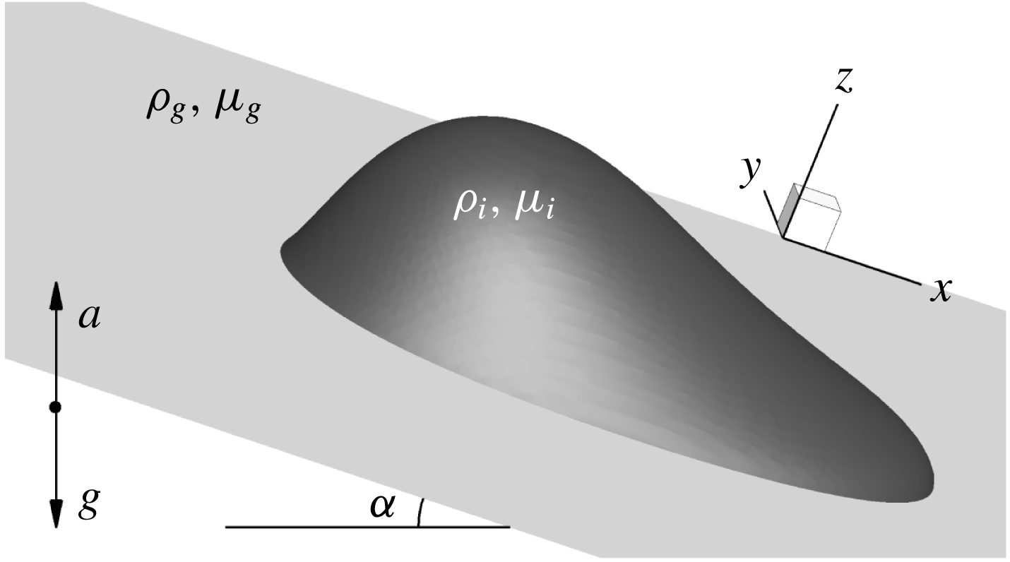
Sketch of a moving drop on an inclined plate that vibrates vertically at an acceleration of
 $a=\unicode[STIX]{x1D706}_{a}a_{0}\sin \unicode[STIX]{x1D719}$
.

In this paper, we investigate the ratchet mechanism of drops climbing a vibrated oblique plate based on three-dimensional (3D) direct numerical simulations, which can reproduce the existing experiment of Brunet et al. (Reference Brunet, Eggers and Deegan2007) with respect to the evolution of drop shapes. This is the first time that the combined effects of vibration, inertia, viscosity, gravity and contact angle hysteresis have been taken into account in 3D numerical simulations. The numerical simulations allow us to access the time variation of the wetted area of the drop, which is difficult to measure in experiments. We find that the drop has a larger wetted area when it slides down than when it moves up. A new hydrodynamic model is proposed based on the balance of the forces exerted on the drop, and shows that the asymmetry of the wetted area is responsible for the uphill net displacement of the drop. The model correlates the net drop velocity with the vibration (both amplitude and frequency), the contact angle hysteresis and the non-harmonic response of the drop, and is verified by comparison with numerical results.
2 Methodology
We solve the 3D Navier–Stokes equations coupled with a diffuse interface model to simulate the dynamics of a liquid drop on an oblique plate vibrated vertically, as depicted in figure 1. The method allows for two-phase flows with large density and viscosity ratios (Ding, Spelt & Shu Reference Ding, Spelt and Shu2007), moving contact lines (CLs) (Ding & Spelt Reference Ding and Spelt2007a
) and contact angle hysteresis (Ding & Spelt Reference Ding and Spelt2008) without using any ad hoc phenomenological models. The liquid–gas interface is represented by the volume fraction of the liquid,
 $C$
, the evolution of which is governed by
 $$\begin{eqnarray}\frac{\unicode[STIX]{x2202}C}{\unicode[STIX]{x2202}t}+\unicode[STIX]{x1D735}\boldsymbol{\cdot }(\boldsymbol{u}C)=\frac{1}{Pe}\unicode[STIX]{x1D6FB}^{2}\unicode[STIX]{x1D713},\end{eqnarray}$$
where the chemical potential
 $\unicode[STIX]{x1D713}$
is defined as
 $$\begin{eqnarray}\unicode[STIX]{x1D713}=C^{3}-1.5C^{2}+0.5C-Cn^{2}\unicode[STIX]{x1D6FB}^{2}C\end{eqnarray}$$
and the Cahn number
 $Cn$
is a dimensionless measure of the thickness of the diffuse interface. Accordingly, the density and viscosity of the fluid can be calculated by
 $\unicode[STIX]{x1D70C}=C\unicode[STIX]{x1D70C}_{l}+(1-C)\unicode[STIX]{x1D70C}_{g}$
and
 $\unicode[STIX]{x1D707}=C\unicode[STIX]{x1D707}_{l}+(1-C)\unicode[STIX]{x1D707}_{g}$
, where the subscripts
 $l$
and
 $g$
denote liquid and gas respectively. The wettability of the substrate is prescribed by the advancing contact angle
 $\unicode[STIX]{x1D703}_{A}$
and the receding contact angle
 $\unicode[STIX]{x1D703}_{R}$
. A geometrical formulation (Ding & Spelt Reference Ding and Spelt2007a
) is used to impose the wetting condition involving the contact angle hysteresis, and serves as the boundary condition for
 $C$
at the solid substrate. At each time step, the local value of the contact angle is first determined after the advection of the diffuse interface (Ding & Spelt Reference Ding and Spelt2007b
). If this value is outside the hysteresis window, either
 $\unicode[STIX]{x1D703}_{A}$
or
 $\unicode[STIX]{x1D703}_{R}$
is prescribed by setting the appropriate value of
 $C$
at a layer of ghost cells below the solid wall; otherwise, the
 $C$
value at the corresponding ghost cells remains unchanged (Ding & Spelt Reference Ding and Spelt2008). It should be noted that this contact angle hysteresis model excludes the mechanism of nonlinear capillary forces suggested by Brunet et al. (Reference Brunet, Eggers and Deegan2007), in which the local contact angle is assumed to be a function of the CL speed when outside the hysteresis window. Unless otherwise stated, in the simulations, the interface is represented by the
 $C=0.5$
contour,
 $Cn$
is set to
 $0.7\unicode[STIX]{x0394}x$
and the Péclet number is chosen as
 $Pe=1/Cn$
, where
 $\unicode[STIX]{x0394}x$
is the mesh size. More details of the numerical implementation can be found in Ding & Spelt (Reference Ding and Spelt2008).
For convenience of computation, all of the governing equations are solved in a non-inertial frame of reference fixed to the plate, which is assumed to be infinitely large (figure 1). As a result, the effect of the harmonic vibration of the plate on the fluids can be modelled by including an additional volumetric force density
 $\unicode[STIX]{x1D706}_{a}\,a_{0}\unicode[STIX]{x1D70C}\sin \unicode[STIX]{x1D719}\,\boldsymbol{j}$
in the Navier–Stokes equations, where
 $a_{0}$
and
 $\unicode[STIX]{x1D706}_{a}$
are the characteristic and dimensionless amplitudes of the acceleration respectively,
 $\unicode[STIX]{x1D719}$
the phase of the acceleration and
 $\boldsymbol{j}$
the vertical unit vector. In the present study, we set
 $a_{0}=174~\text{m}~\text{s}^{-2}$
to be consistent with the experiments by Brunet et al. (Reference Brunet, Eggers and Deegan2007) and choose
 $V^{1/3}$
and
 $a_{0}^{1/2}V^{1/6}$
as the characteristic length and velocity respectively. The dynamics of the drop motion can be represented by a group of dimensionless parameters, namely the Weber number
 $We$
(
 $=\unicode[STIX]{x1D70C}_{l}a_{0}V^{2/3}/\unicode[STIX]{x1D70E}$
), the Reynolds number
 $Re$
(
 $=\unicode[STIX]{x1D70C}_{l}a_{0}^{1/2}V^{1/2}/\unicode[STIX]{x1D707}_{l}$
), the Froude number
 $Fr$
(
 $=\sqrt{a_{0}/g}$
) and the Strouhal number
 $St$
(
 $=\unicode[STIX]{x1D701}V^{1/6}a_{0}^{-1/2}$
), where
 $\unicode[STIX]{x1D70E}$
is the surface tension,
 $V$
is the drop volume and
 $\unicode[STIX]{x1D701}$
is the vibration frequency. Thus, the phase
 $\unicode[STIX]{x1D719}$
is related to the dimensionless time
 $t$
by
 $\unicode[STIX]{x1D719}=2\unicode[STIX]{x03C0}St\cdot t$
. A fixed inclination angle (
 $\unicode[STIX]{x1D6FC}=45^{\circ }$
) is considered, and the density and viscosity ratios of the gas to the liquid are 0.001 and 0.01 respectively.
In all of the calculations reported here, half of the drop has been simulated in a domain of
 $6\times 2\times 2$
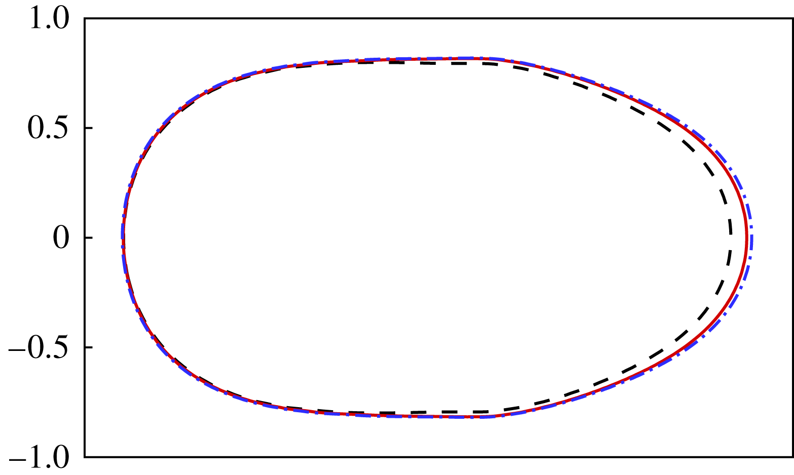
on a uniform Cartesian mesh. Figure 3 shows the grid-independence study with respect to the CL shape at
 $\unicode[STIX]{x1D719}=7/10\unicode[STIX]{x03C0}$
for three different mesh sizes (
 $\unicode[STIX]{x0394}x=1/40$
,
 $1/60$
and
 $1/70$
). We can see that the results with
 $\unicode[STIX]{x0394}x=1/60$
and
 $1/70$
are virtually overlapped. Therefore, in the following, we use the Cartesian mesh with
 $\unicode[STIX]{x0394}x=1/60$
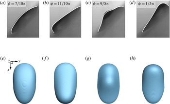
in the simulations. The method is also validated by comparing with the experimental data of Brunet et al. (Reference Brunet, Eggers and Deegan2007) (figure 2
a), and, clearly, good agreement has been achieved on the evolution of the drop shape. On the other hand, the dimensionless net drop velocity,
 $U_{m}$
, is approximately
 $0.008$
in the numerical simulation, which is of the same order as but faster than the experimental result (i.e. 1.79 mm
 $\text{s}^{-1}$
or
 $U_{m}\approx 0.003$
). This is mainly because of the limitation of computational capability. For the millimetre-sized drops considered here, the slip length at the CL is
 ${\sim}10~\unicode[STIX]{x03BC}\text{m}$
in the simulation (Ding & Spelt Reference Ding and Spelt2007a
), which falls short of realistic conditions, e.g.
 ${\sim}O(0.1~\unicode[STIX]{x03BC}\text{m})$
(Marsh, Garoff & Dussan Reference Marsh, Garoff and Dussan1993), thereby leading to the faster displacement of the drop.
3 Results and discussion
Snapshots of a climbing drop at different phases with
 $Re=30.9$
,
 $We=9.17$
,
 $St=0.185$
,
 $Fr=17.8$
,
 $\unicode[STIX]{x1D706}_{a}=1.03$
,
 $\unicode[STIX]{x1D703}_{A}=77^{\circ }$
,
 $\unicode[STIX]{x1D703}_{R}=44^{\circ }$
and
 $\unicode[STIX]{x1D6FC}=45^{\circ }$
. (a–d) Comparison with the experimental data obtained by Brunet et al. (Reference Brunet, Eggers and Deegan2007) under the same flow conditions. Side views of the drop from the numerical results (white curves) are superimposed on the experimental snapshots. (e–h) Top view of the drop shape in the numerical simulations at the same phases as in (a–d).

Convergence study for the shape of the CL at
 $\unicode[STIX]{x1D719}=7/10\unicode[STIX]{x03C0}$
. The flow parameters are the same as in figure 2. The numerical results are obtained on meshes of different resolutions:
 $\unicode[STIX]{x0394}x=1/40$
(dashed),
 $1/60$
(solid) and
 $1/70$
(dash-dotted).

3.1 The dynamics of a climbing drop
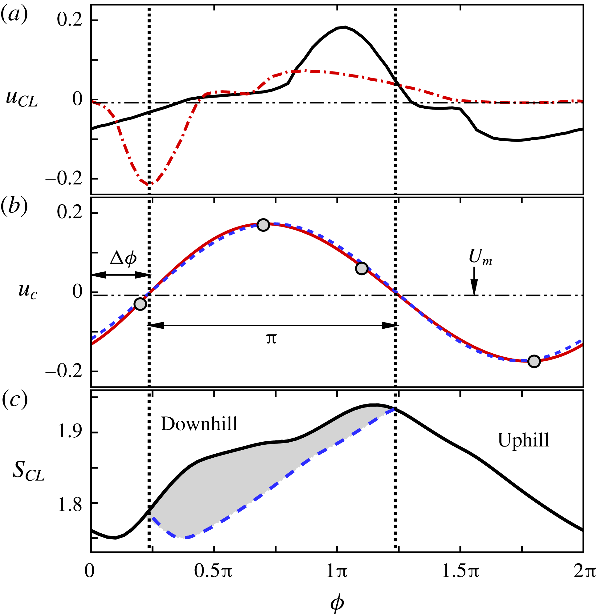
Figure 2 shows snapshots of a climbing drop at different phases. We can see that the drop motion is accompanied by a capillary wave travelling at the surface of the drop. The capillary wave is more noticeable when the drop moves up than when it slides down. The interaction between the capillary wave and the CL results in complicated CL motion at the upper and lower ends of the drop in one period of acceleration (figure 4
a), and the CL speed
 $u_{CL}$
reaches its maximum value at roughly
 $\unicode[STIX]{x1D719}=1/4\unicode[STIX]{x03C0}$
for the upper end and
 $\unicode[STIX]{x1D719}=\unicode[STIX]{x03C0}$
for the lower end. By contrast, the variation of the volume-averaged
 $x$
component of the drop velocity,
 $u_{c}=(1/V)\int _{\unicode[STIX]{x1D6FA}(t)}u\,\text{d}\unicode[STIX]{x1D6FA}$
, is close to a harmonic function with a shift of
 $U_{m}$
(figure 4
b), where
 $u$
is the projection of the fluid velocity
 $\boldsymbol{u}$
on the
 $x$
-axis and
 $\unicode[STIX]{x1D6FA}(t)$
is the space occupied by the drop at time
 $t$
. The oscillation of the drop on the plate has the same frequency as the acceleration but experiences a delay of
 $\unicode[STIX]{x0394}\unicode[STIX]{x1D719}$
in phase due to the inertia of the drop. Therefore, we can quantitatively divide the drop motion in one period into two stages of equal phase interval: the downhill stage [
 $\unicode[STIX]{x0394}\unicode[STIX]{x1D719},\,\unicode[STIX]{x03C0}+\unicode[STIX]{x0394}\unicode[STIX]{x1D719}$
] and the uphill stage [
 $\unicode[STIX]{x03C0}+\unicode[STIX]{x0394}\unicode[STIX]{x1D719},\,2\unicode[STIX]{x03C0}+\unicode[STIX]{x0394}\unicode[STIX]{x1D719}$
] (figure 4
b). We can see that figures 2(e) and 2(g) correspond to the drop shapes with the maximum average speed of motion downhill and uphill respectively. Their difference indicates the fore–aft asymmetry of drop deformation during its oscillation on the substrate. Figure 4(c) shows the evolution of the wetted area of the drop,
 $S_{CL}$
. We find that the broken symmetry causes a non-harmonic variation in the wetted area, thereby leading to a hysteresis loop of the wetted area in one period. In particular, the average wetted area in the downhill stage is larger than that in the uphill stage. This will be shown to induce the net uphill displacement of the drop.
The variation of the flow quantities in one period of acceleration. It should be noted that this is the same case as in figure 2. (a) The variation of the CL speed
 $u_{CL}$
at the upper end (dash-dotted line) and lower end (solid line) of the CL. (b) The variation of the volume-averaged drop velocity
 $u_{c}$
(solid line), which is close to a harmonic function (dotted line). The bullets indicate the corresponding phases shown in figure 2. (c) The non-harmonic variation of the wetted area
 $S_{CL}$
. The dashed line represents an image of the variation of the wetted area in the uphill stage. The region in grey corresponds to the difference in the wetted area between the uphill and downhill stages in one period, i.e.
 $\unicode[STIX]{x03C0}\cdot \unicode[STIX]{x0394}S$
.

3.2 The forces exerted on the drop
We analyse here the forces acting on the drop, in order to interpret the ratchet mechanism that causes the net uphill movement of the drop. These forces consist of the contributions from the plate (i.e. capillary force at the CL, viscous force and plate vibration), gravity and the surrounding gas. Among them, we can neglect the force exerted by the gas. It is primarily due to the low density and viscosity of the gas and the insignificant difference in velocity between the drop and the surrounding gas. Hence, the variation of drop momentum in a dimensionless form yields
 $$\begin{eqnarray}\int _{\unicode[STIX]{x1D6FA}}\frac{\text{D}\boldsymbol{u}}{\text{D}t}\,\text{d}V=\frac{1}{Re}\int _{S_{CL}}\boldsymbol{n}_{w}\boldsymbol{\cdot }\unicode[STIX]{x1D64F}\,\text{d}S+\frac{1}{We}\oint _{CL}\unicode[STIX]{x1D749}\,\text{d}l+\int _{\unicode[STIX]{x1D6FA}}\left(\unicode[STIX]{x1D706}_{a}\sin \unicode[STIX]{x1D719}+\frac{1}{Fr^{2}}\right)\boldsymbol{j}\,\text{d}V,\end{eqnarray}$$
where
 $\boldsymbol{n}_{w}$
denotes the unit vectors normal to the wall and pointing away from the drop,
 $\unicode[STIX]{x1D64F}$
is the stress tensor and
 $\unicode[STIX]{x1D749}$
is the unit vector tangential to the interface in the plane spanned by the vectors normal to the substrate and to the CL.
The effect of the gravitational force simply prompts the drop to slide down, and it has been experimentally shown that it does not contribute to the uphill motion of the drop (Brunet et al. Reference Brunet, Eggers and Deegan2007). Therefore, in the following studies, we rule out the gravitational force and mainly focus on the role of the forces exerted by the plate in the uphill net displacement of the drop, or, more specifically, the role of the viscous force, the volumetric force due to plate vibration and the capillary force arising from contact angle hysteresis.
For convenience of analysis, we define the time average of any quantity
 $q$
over the downhill or uphill stage by
 $$\begin{eqnarray}\langle q\rangle _{M}=\frac{2}{T}\int _{T/2}q\,\text{d}t,\end{eqnarray}$$
where the subscript
 $M$
can be up or down, corresponding to the uphill and downhill stages respectively.
3.3 The ratchet mechanism of drop climbing
We first consider cases in the absence of contact angle hysteresis, i.e.
 $(1/We)\oint _{CL}\unicode[STIX]{x1D749}\,\text{d}l\approx 0$
. Integration of the
 $x$
component of (3.1) over one period suggests that the time average of the viscous force exerted by the wall should be approximately zero, or
 $\langle f_{v}\rangle _{up}+\langle f_{v}\rangle _{down}\approx 0$
, where
 $f_{v}$
is the
 $x$
component of the viscous force. We tentatively write the average viscous force
 $\langle f_{v}\rangle$
as
 $-\unicode[STIX]{x1D6FD}\langle u_{c}\rangle \langle S_{CL}\rangle /Re$
, where
 $\unicode[STIX]{x1D6FD}$
is a positive coefficient that relates to the distribution of shear strain near the wall. Assuming that the value of
 $\unicode[STIX]{x1D6FD}$
is roughly the same in the uphill and downhill stages, we can obtain
 $$\begin{eqnarray}\displaystyle \langle u_{c}\rangle _{up}\langle S_{CL}\rangle _{up}+\langle u_{c}\rangle _{down}\langle S_{CL}\rangle _{down}\approx 0. & & \displaystyle\end{eqnarray}$$
For simplicity, we define
 $S_{m}=(\langle S_{CL}\rangle _{up}+\langle S_{CL}\rangle _{down})/2$
and
 $\unicode[STIX]{x0394}S=\langle S_{CL}\rangle _{down}-\langle S_{CL}\rangle _{up}$
(as illustrated in figure 4
b). Then, taking the net velocity of the drop
 $U_{m}=(\langle u_{c}\rangle _{up}+\langle u_{c}\rangle _{down})/2$
into account and assuming
 $\unicode[STIX]{x0394}S^{2}\ll S_{m}^{2}$
, (3.3) can be rewritten as
 $$\begin{eqnarray}\displaystyle -U_{m}\approx \langle f_{v}\rangle _{down}\frac{Re}{\unicode[STIX]{x1D6FD}}\frac{\unicode[STIX]{x0394}S}{S_{m}^{2}}. & & \displaystyle\end{eqnarray}$$
On the other hand, we note that the drop momentum has the same value at the start and end of the downhill (and also uphill) stage (see figure 4
a). This implies that the viscous force should be balanced by the volumetric force arising from the plate acceleration during the downhill (and uphill) stage. Integration of the
 $x$
component of (3.1) over the period of the downhill stage yields
 $$\begin{eqnarray}\displaystyle \langle f_{v}\rangle _{down}=\frac{2\unicode[STIX]{x1D706}_{a}}{\unicode[STIX]{x03C0}}\sin \unicode[STIX]{x1D6FC}\cos \unicode[STIX]{x0394}\unicode[STIX]{x1D719}. & & \displaystyle\end{eqnarray}$$
By substituting (3.5) into (3.4), we can obtain a quantitative estimate of the net drop velocity,
 $$\begin{eqnarray}\displaystyle Ca\propto \unicode[STIX]{x1D706}_{a}\cos \unicode[STIX]{x0394}\unicode[STIX]{x1D719}\,We\,\sin \unicode[STIX]{x1D6FC}\,\frac{\unicode[STIX]{x0394}S}{S_{m}^{2}}, & & \displaystyle\end{eqnarray}$$
where
 $Ca=-U_{m}\,\unicode[STIX]{x1D707}\sqrt{a_{0}V^{1/3}}/\unicode[STIX]{x1D70E}$
. We can conclude from (3.6) that in the absence of contact angle hysteresis, the drop will always move uphill with
 $\unicode[STIX]{x0394}S>0$
and
 $\unicode[STIX]{x0394}\unicode[STIX]{x1D719}<\unicode[STIX]{x03C0}/2$
. The term
 $\unicode[STIX]{x0394}S/S_{m}^{2}$
represents the non-harmonic response of the drop to the spatial asymmetry and vibration, and thus is directly related to the mobility of the drop. This explains the experimental observations of Sartori et al. (Reference Sartori, Quagliati, Varagnolo, Pierno, Mistura, Magaletti and Casciola2015), namely that it is more likely for a drop to move uphill on a hydrophobic substrate than a hydrophilic one. For a drop of fixed volume, the more hydrophobic the substrate is, the smaller
 $S_{m}$
is, and thus the higher the drop mobility is.
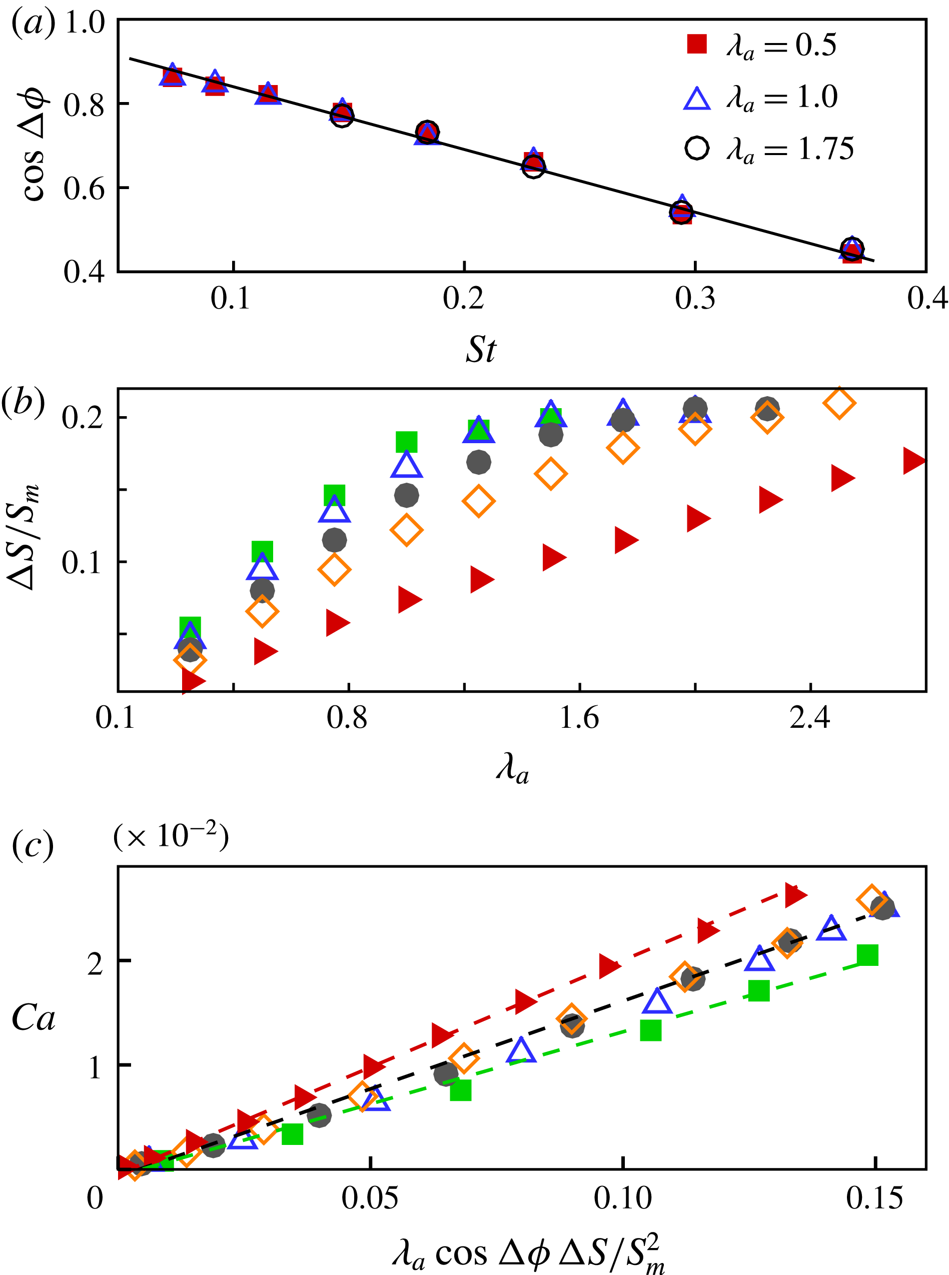
Numerical results in the absence of gravity and contact angle hysteresis (
 $\unicode[STIX]{x1D703}_{A}=\unicode[STIX]{x1D703}_{R}=60^{\circ }$
) at
 $We=6.6$
and
 $Re=23.6$
. (a) The variation of
 $\cos \unicode[STIX]{x0394}\unicode[STIX]{x1D719}$
as a function of
 $St$
. The solid line is a linear fitting of the data. (b) The variation of
 $\unicode[STIX]{x0394}S/S_{m}$
as a function of
 $\unicode[STIX]{x1D706}_{a}$
. (c) Comparison of the net drop velocity between numerical results and the predictions of (3.6); the dashed lines represent linear fittings. It should be noted that the same cases are included in (b) and (c), with
 $St=0.115$
(▪), 0.148 (▵), 0.184 (●), 0.231 (♢) and 0.294 (▸).

Numerical experiments are performed to verify the theoretical prediction of (3.6). Figure 5 shows the numerical results for a variety of values of
 $\unicode[STIX]{x1D706}_{a}$
and
 $St$
, and several observations can be made. First, correlation is only seen between
 $\unicode[STIX]{x0394}\unicode[STIX]{x1D719}$
and
 $St$
; this is reasonable since
 $\unicode[STIX]{x0394}\unicode[STIX]{x1D719}$
reflects the temporal response of the drop inertia to variation of the acceleration. In addition,
 $\cos \unicode[STIX]{x0394}\unicode[STIX]{x1D719}$
appears to decrease linearly with increase of
 $St$
in the parameter space considered (figure 5
a). Second,
 $\unicode[STIX]{x0394}S/S_{m}$
linearly increases with
 $\unicode[STIX]{x1D706}_{a}$
for a relatively small amplitude of vibration (
 $\unicode[STIX]{x1D706}_{a}<1$
) and the slope is dependent on
 $St$
: the higher the frequency of the plate vibration is, the gentler the slope is. For sufficiently large
 $\unicode[STIX]{x1D706}_{a}$
,
 $\unicode[STIX]{x0394}S/S_{m}$
approaches a maximum value (
 ${\sim}20\,\%$
), which is independent of
 $St$
. Figure 5(c) shows a comparison of
 $Ca$
between the numerical results and the theoretical prediction, and good agreement has been obtained. The results at
 $St=0.148$
,
 $0.184$
and
 $0.231$
nearly collapse onto a single line, probably because the frequency of the acceleration in these cases is close to the resonance frequency of the drop, i.e.
 $f=63$
Hz or
 $St=0.185$
(Celestini & Kofman Reference Celestini and Kofman2006). For the other two cases (
 $St=0.115$
and
 $0.294$
), (3.6) remains valid, but the proportion factors are apparently different. This implies that the value of
 $\unicode[STIX]{x1D6FD}$
may also be a function of the frequency of the plate vibration. Overall, our numerical experiments confirm the prediction of (3.6).
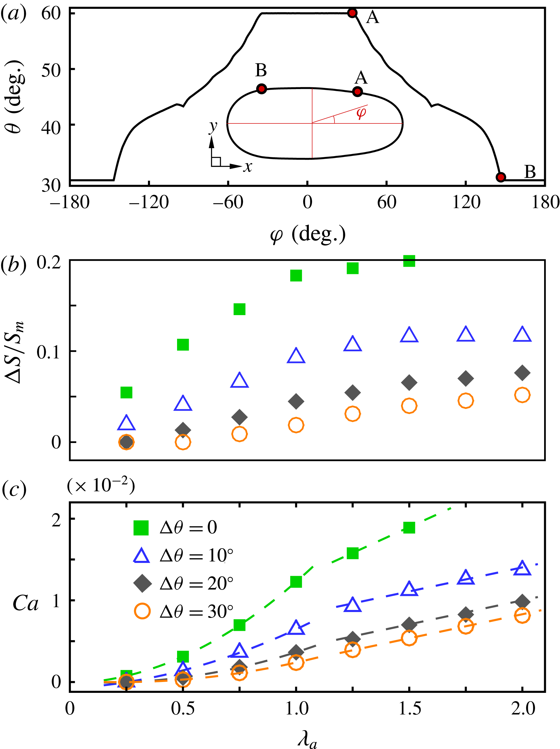
Numerical results in the absence of gravity at
 $We=6.6$
,
 $Re=23.6$
and
 $\unicode[STIX]{x1D703}_{A}=60^{\circ }$
. (a) The contact angle distribution at
 $\unicode[STIX]{x1D719}=\unicode[STIX]{x03C0}$
, with
 $St=0.148$
,
 $\unicode[STIX]{x1D706}_{a}=1.75$
and
 $\unicode[STIX]{x1D703}_{R}=30^{\circ }$
. (b,c) The same cases at
 $St=0.115$
; the results are denoted by the same symbols. The variation of
 $\unicode[STIX]{x0394}S/S_{m}$
and the net drop velocity
 $Ca$
at different values of
 $\unicode[STIX]{x0394}\unicode[STIX]{x1D703}$
are shown in (b) and (c) respectively. The dashed lines in (c) represent data fittings (quadratic for
 $\unicode[STIX]{x1D706}_{a}\leqslant 1$
and linear for
 $\unicode[STIX]{x1D706}_{a}\geqslant 1.25$
).

3.4 The role of contact angle hysteresis
We further analyse the role of contact angle hysteresis,
 $\unicode[STIX]{x0394}\unicode[STIX]{x1D703}$
(
 $=\unicode[STIX]{x1D703}_{A}-\unicode[STIX]{x1D703}_{R}$
), in the drop motion. First, contact angle hysteresis gives rise to the capillary force at the CL that is against drop displacement, e.g. subject to the shear force from the surrounding fluid (Ding, Gilani & Spelt Reference Ding, Gilani and Spelt2010) or the gravitational force (Podgorski, Flesselles & Limat Reference Podgorski, Flesselles and Limat2001). The magnitude of the capillary force depends on the distribution of the contact angle along the CL. A typical case is shown in figure 6(a), where the local contact angle on the sides of the CL mainly falls in the range
 $\unicode[STIX]{x1D703}_{R}<\unicode[STIX]{x1D703}<\unicode[STIX]{x1D703}_{A}$
. Therefore, the capillary force can be approximated by
 $(\cos \unicode[STIX]{x1D703}_{R}-\cos \unicode[STIX]{x1D703}_{A})W_{CL}\,We^{-1}$
, where
 $W_{CL}$
is the dimensionless width of the CL. We can expect that the drop stays in the static regime for low acceleration such that
 $\unicode[STIX]{x1D706}_{a}We\,(\cos \unicode[STIX]{x1D703}_{R}-\cos \unicode[STIX]{x1D703}_{A})^{-1}\sim O(1)$
, in which the vibration is not strong enough to depin the CL. This is confirmed by numerical results in figure 6(c), and the threshold value of
 $\unicode[STIX]{x1D706}_{a}$
increases with
 $\unicode[STIX]{x0394}\unicode[STIX]{x1D703}$
(
 $\unicode[STIX]{x1D706}_{a}\sim 0.25$
at
 $\unicode[STIX]{x0394}\unicode[STIX]{x1D703}=10^{\circ }$
and
 ${\sim}0.5$
at
 $\unicode[STIX]{x0394}\unicode[STIX]{x1D703}=30^{\circ }$
).
Second, contact angle hysteresis tends to reduce the drop mobility. Under extreme conditions such as
 $\unicode[STIX]{x1D703}_{A}=180^{\circ }$
and
 $\unicode[STIX]{x1D703}_{R}=0^{\circ }$
, in principle, the CL would be completely pinned, regardless of the acceleration amplitude. Numerical results in figure 6(b) show that
 $\unicode[STIX]{x0394}S/S_{m}$
decreases significantly with increase of
 $\unicode[STIX]{x0394}\unicode[STIX]{x1D703}$
. We can observe that
 $\unicode[STIX]{x0394}S/S_{m}$
changes linearly with
 $\unicode[STIX]{x1D706}_{a}$
for
 $\unicode[STIX]{x1D706}_{a}\leqslant 1$
and remains at roughly the same value for
 $\unicode[STIX]{x1D706}_{a}\geqslant 1.25$
; interestingly, a transition of net drop velocity occurs simultaneously (figure 6
c). For relatively large
 $\unicode[STIX]{x1D706}_{a}$
, the vibration depins the CL, especially at the upper and lower parts. Since the variation of
 $W_{CL}$
is insignificant (see figure 2
e–h), it can be assumed that the capillary forces in the uphill and downhill stages cancel each other out. Consequently, the transition of
 $Ca$
with
 $\unicode[STIX]{x1D706}_{a}$
in the presence of contact angle hysteresis can be well predicted by (3.6). Specifically, we can obtain
 $Ca\propto \unicode[STIX]{x1D706}_{a}^{2}$
for
 $0.5\leqslant \unicode[STIX]{x1D706}_{a}\leqslant 1$
and
 $Ca\propto \unicode[STIX]{x1D706}_{a}$
for
 $\unicode[STIX]{x1D706}_{a}\geqslant 1.25$
, in agreement with numerical results (figure 6
c). This transition of
 $Ca$
with
 $\unicode[STIX]{x1D706}_{a}$
was also observed in experiments (Brunet et al.
Reference Brunet, Eggers and Deegan2007) in a similar range of
 $\unicode[STIX]{x1D706}_{a}$
(
 ${\sim}1\,-\,1.2$
), accompanied by a change of wetting behaviour at the trailing end of the drop.
4 Conclusion and perspectives
In summary, we have investigated the ratchet mechanism of a drop climbing a vibrated oblique plate based on numerical simulations that are verifiable with experiments. We found that the spatial asymmetry causes a non-harmonic response of the wetted area to the harmonic acceleration, and, in particular,
 $\langle S_{CL}\rangle _{down}>\langle S_{CL}\rangle _{up}$
. A new hydrodynamic model has been developed, to associate the net drop velocity with the acceleration, drop mobility, inertia, viscosity and contact angle hysteresis. This model suggests that the hysteresis loop of the wetted area represents the effect of a ratchet mechanism, and that the resultant nonlinear viscous force accounts for the net displacement of the drop. The prediction of the model was verified by numerical simulations. Although the contact angle hysteresis is apparently reduced by sufficiently strong vibration (Daniel et al.
Reference Daniel, Sircar, Gliem and Chaudhury2004; Brunet et al.
Reference Brunet, Eggers and Deegan2007), it was found to significantly affect the variation of the net drop velocity with the acceleration amplitude.
The presence of gravity makes the drop prone to sliding down the inclined plate. Since gravity is much smaller than the acceleration of the plate (such that
 $\unicode[STIX]{x1D706}_{a}^{2}Fr^{2}\gg 1$
), it is supposed to have little effect on the drop shape, as experimentally confirmed by Brunet et al. (Reference Brunet, Eggers and Deegan2007). It is also reasonable to expect that the gravitational force would not affect the wetted area of the drop either. As a result, the drop can appropriately adjust its net velocity
 $U_{m}$
in such a way that the gravitational force is eventually balanced by the resultant upward net viscous force exerted by the plate. Furthermore, a nonlinear capillary force and a nonlinear viscous force may coexist in the ratchet mechanism of net uphill drop motion. It would be interesting to know which of the two is more important under a particular set of conditions. For this purpose, a dynamic contact angle model is required in the numerical simulation. This is beyond the scope of the present study but will be the focus of our future research.
Acknowledgements
We are grateful for the support of the National Natural Science Foundation of China (grant nos. 11425210, 11621202, 11672288), the Strategic Priority Research Program of the Chinese Academy of Sciences (grant no. XDB22040103) and the Fundamental Research Funds for the Central Universities.