1 Introduction
Magnetic reconnection is a fundamental process which causes magnetic field lines to change their topological connectivity over a diffusive region due to non-ideal magnetohydrodynamic (MHD) effects such as the plasma resistivity (Priest & Forbes Reference Priest and Forbes2009; Yamada, Kulsrud & Ji Reference Yamada, Kulsrud and Ji2010). Magnetic reconnection has generally been understood as a suitable mechanism to accelerate protons and electrons in some astrophysical contexts, especially, in solar flares (Goldstein, Matthaeus & Ambrosiano Reference Goldstein, Matthaeus and Ambrosiano1986; Benz, Grigis & Battaglia Reference Benz, Grigis and Battaglia2006; Knizhnik, Swisdak & Drake Reference Knizhnik, Swisdak and Drake2011; Lin Reference Lin2011). Observing the solar corona, Ramaty High Energy Solar Spectroscopic Imager (RHESSI) detection instruments have measured a large number of accelerated protons and electrons with energies of the order of keV and MeV (Lin et al. Reference Lin2003).
Non-ideal diffusive regions, where magnetic reconnection takes place in three dimensions, have been thought to be the source of accelerated particles. While in two dimensions, reconnection takes place at an X-type magnetic null point within a localized diffusive region, in three dimensions it may also take place at null points or along separators or at locations where the magnetic field does not vanish, called non-null points (Priest & Pontin Reference Priest and Pontin2009; Pontin Reference Pontin2011; Pontin, Al-Hachami & Galsgaard Reference Pontin, Al-Hachami and Galsgaard2011). Spine and fan reconnection models assume that the reconnection takes place at null points and a strong current is flowing either along the spine axis (spine regime) or on the fan plane (fan regime). However, the non-null reconnection proceeds in localized non-ideal region where a non-zero electric field component parallel to the magnetic field exists. Therefore, such a type of reconnection may proceed without the presence of a null-point.
In the steady-state kinematic model of the non-null reconnection presented by Hornig & Priest (Reference Hornig and Priest2003), solutions of the incompressible MHD equations with a localized resistive diffusion region have been given. An X-type magnetic field in the
 $x{-}y$
plane was added to a uniform field in the
 $z$
-direction. Then, the resistive Ohm’s law imposes a particular solutions for the electric field and velocity called pure solutions. In the study of Wilmot-Smith, Hornig & Priest (Reference Wilmot-Smith, Hornig and Priest2006), the momentum equation has also been taken into the system of MHD equations. Our present study is based on the pure reconnection solutions for the perturbed electric and magnetic fields modelled in the latter study.
Recently, we investigated test particle acceleration in torsional spine and torsional fan reconnection regimes; two important three-dimensional reconnection types with a null point (Hosseinpour Reference Hosseinpour2014a ,Reference Hosseinpour b ). By adopting typical parameters for the solar corona, we found that a proton can be accelerated to MeV and even higher kinetic energies in less than a few milliseconds. Its trajectory and final energy strongly depend on its initial injection position around a null point; acceleration along the spine axis, on the fan plane or trapping around the null point are three possible scenarios for the proton trajectory. In our most recent study (Hosseinpour Reference Hosseinpour2015) we injected a population of 10 000 protons and concluded that almost half of the injected protons were accelerated in the form of two similar jets above and below the flan plane and most of the other half of the population were accelerated on the fan plane. Moreover, a considerable fraction of particles gained MeV kinetic energies. Now, it is of interest to investigate the same problem of proton acceleration in a different, but important, type of three-dimensional reconnection which is non-null-point reconnection. It is interesting to see whether jets of energetic protons can again be produced in this non-null type of reconnection and whether a considerable fraction of protons can reach MeV kinetic energies or not.
Thus, by considering a kinematic model of non-null reconnection, we investigate the trajectory and energy distribution for a population of 10 000 protons which are randomly distributed within a cubic space around a non-null point with typical parameters for the solar corona. These test protons move only due to the force of electric and magnetic fields.
The non-null-point reconnection model is briefly outlined in § 2 with a description of the ‘trajectory code’. Results and discussion regarding the particle acceleration and energy distribution are given in § 3. Finally, a brief conclusion is presented in § 4.
2 Non-null-point reconnection model
As mentioned, the present analysis builds on a three-dimensional non-null reconnection type demonstrated in detail by Wilmot-Smith et al. (Reference Wilmot-Smith, Hornig and Priest2006). According to this study, solutions of the following steady-state resistive MHD equations
 $$\begin{eqnarray}\displaystyle & \boldsymbol{E}+\boldsymbol{V}\times \boldsymbol{B}=\unicode[STIX]{x1D702}\boldsymbol{J}, & \displaystyle\end{eqnarray}$$
 $$\begin{eqnarray}\displaystyle & \unicode[STIX]{x1D735}\times \boldsymbol{E}=0, & \displaystyle\end{eqnarray}$$
 $$\begin{eqnarray}\displaystyle & \unicode[STIX]{x1D735}\times \boldsymbol{B}=\unicode[STIX]{x1D707}_{0}\boldsymbol{J}, & \displaystyle\end{eqnarray}$$
 $$\begin{eqnarray}\displaystyle & \unicode[STIX]{x1D735}\boldsymbol{\cdot }\boldsymbol{B}=0, & \displaystyle\end{eqnarray}$$
are obtained by expanding the variable quantities in powers of the Alfvén Mach number
 $M\equiv v/v_{A}<1$
, where
 $v$
and
 $v_{A}$
are the plasma flow and the Alfvén speed, respectively:
 $$\begin{eqnarray}\left.\begin{array}{@{}c@{}}\boldsymbol{B}=\boldsymbol{B}_{0}+M\boldsymbol{B}_{1}+M^{2}\boldsymbol{B}_{2}+\cdots \\ \boldsymbol{E}=\boldsymbol{E}_{0}+M\boldsymbol{E}_{1}+M^{2}\boldsymbol{E}_{2}+\cdots \\ \boldsymbol{v}=\boldsymbol{v}_{1}+M\boldsymbol{v}_{2}+M^{2}\boldsymbol{v}_{3}+\cdots \\ \boldsymbol{J}=M\boldsymbol{J}_{1}+M^{2}\boldsymbol{J}_{2}+\cdots \,.\end{array}\right\}\end{eqnarray}$$
The equilibrium magnetic field is given by
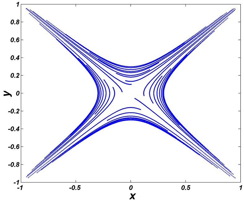
 $$\begin{eqnarray}\boldsymbol{B}_{0}=b_{0}(ky,kx,1),\end{eqnarray}$$
which has an X-type structure in the
 $x{-}y$
plane. Here,
 $k$
is a positive constant. Figures 1 and 2 plot some typical field lines for
 $\boldsymbol{B}_{0}$
with
 $k=0.5$
. Wilmot-Smith et al. (Reference Wilmot-Smith, Hornig and Priest2006) found pure reconnection solutions by inserting the expansions of (2.5) into both Ohm’s law and the equation of motion. Then, the terms with the same power of
 $M$
were compared with further assumptions of
 $\boldsymbol{v}_{1}=0$
and
 $\boldsymbol{E}_{0}=0$
. Moreover, to ensure the zeroth-order flow was ideal, it was assumed that
 $\boldsymbol{B}_{1}=0$
. According to the solutions presented by Wilmot-Smith et al. (Reference Wilmot-Smith, Hornig and Priest2006) for the case of a uniform current,
 $\boldsymbol{J}_{2}=J_{20}\hat{z}$
, the perturbed magnetic and electric fields are
 $$\begin{eqnarray}\boldsymbol{B}_{2}=-J_{20}y\hat{x},\end{eqnarray}$$
 $$\begin{eqnarray}\displaystyle \boldsymbol{E}_{1} & = & \displaystyle Q\,\text{e}^{\unicode[STIX]{x1D6FE}}\frac{(x\cosh (2kz)+y\sinh (2kz))}{l}\hat{x}+Q\,\text{e}^{\unicode[STIX]{x1D6FE}}\frac{(x\sinh (2kz)-y\cosh (2kz))}{l}{\hat{y}}\nonumber\\ \displaystyle & & \displaystyle +\,\left(Q\text{e}^{\unicode[STIX]{x1D6FE}}\frac{(2kxy\cosh (2kz)-k(x^{2}+y^{2})\sinh (2kz))}{l}+e_{0}\text{e}^{\unicode[STIX]{x1D6FE}}\text{e}^{-z^{2}/L^{2}}\right)\hat{z},\end{eqnarray}$$
with
 $$\begin{eqnarray}Q=\frac{e_{0}\sqrt{\unicode[STIX]{x03C0}}L}{l}\text{erf}\left(\frac{z}{L}\right),\end{eqnarray}$$
and
 $$\begin{eqnarray}\unicode[STIX]{x1D6FE}=-\frac{(x^{2}+y^{2})\cosh (2kz)-2xy\sinh (2kz)}{l^{2}}.\end{eqnarray}$$
The parameters
 $L$
and
 $l$
determine the length and width of the diffusion region, respectively. The equilibrium X-type configuration in the
 $x{-}y$
plane is maintained with this perturbation of magnetic field:
 $\boldsymbol{B}_{0}+M^{2}\boldsymbol{B}_{2}$
. However, it has separatrices inclined at a different angle.
Three-dimensional plot of magnetic field lines for equilibrium magnetic field given by (2.6).

Two-dimensional plot of magnetic field lines for equilibrium magnetic field given by (2.6).

Now, given the magnetic and electric fields,
 $\boldsymbol{B}=\boldsymbol{B}_{0}+M^{2}\boldsymbol{B}_{2}$
,
 $\boldsymbol{E}=M\boldsymbol{E}_{1}$
, we can study particle acceleration by solving the equations of motion of a particle:
 $$\begin{eqnarray}\displaystyle & \displaystyle \frac{\text{d}\boldsymbol{x}}{\text{d}t}=\frac{\boldsymbol{p}}{m_{0}\unicode[STIX]{x1D6FE}_{v}}, & \displaystyle\end{eqnarray}$$
 $$\begin{eqnarray}\displaystyle & \displaystyle \frac{\text{d}\boldsymbol{p}}{\text{d}t}=q\left(\boldsymbol{E}+\frac{\boldsymbol{p}}{m_{0}\unicode[STIX]{x1D6FE}_{v}}\times \boldsymbol{B}\right). & \displaystyle\end{eqnarray}$$
Here
 $t$
is time,
 $\boldsymbol{x}$
and
 $\boldsymbol{p}$
are the particle’s position and momentum vectors and
 $q$
and
 $m_{0}$
are its electric charge and rest mass. Also
 $\unicode[STIX]{x1D6FE}_{v}=1/\sqrt{1-v^{2}/c^{2}}$
. The ‘trajectory code’ computationally solves (2.11) and (2.12) by using the ‘ODE.f90’ routine to solve a system of ordinary differential equations (Shampine & Gordon Reference Shampine and Gordon975).
We have normalized length scales to the characteristic length
 $L=10~\text{km}$
, a typical scale in the solar corona, and the magnetic field by
 $b_{0}=0.01T$
, typical of an active region. Additionally, time is normalized by the gyro-period of a proton, namely,
 $T=2\unicode[STIX]{x03C0}m_{0}/(qb_{0})$
i.e.
 $T\approx 6.5~\unicode[STIX]{x03BC}\text{s}$
.
3 Results and discussion
At
 $t=0$
, we randomly inject 10 000 protons in the vicinity of a non-null point inside a region defined by
 $x=-1:1$
,
 $y=-1:1$
,
 $z=-1:1$
(in dimensionless units). Then, up to a final time of 2000, the trajectory of each proton is calculated by integrating (2.11) and (2.12). At this time, which corresponds to approximately 13 ms, almost all of the protons reach a constant kinetic energy. On the other hand, the injection velocities of the particles are isotropically randomized according to a Maxwellian distribution with a mean temperature of
 $T=86~\text{eV}$
(
 ${\sim}10^{6}~\text{K}$
) corresponding to a mean thermal speed of
 $v_{ave}\sim 1.3\times 10^{5}~\text{m}~\text{s}^{-1}$
. Here, we set
 $L=1$
,
 $l=1$
,
 $k=0.5$
,
 $M=0.01$
and the values of
 $b_{0}$
and
 $e_{0}$
vary as mentioned below.
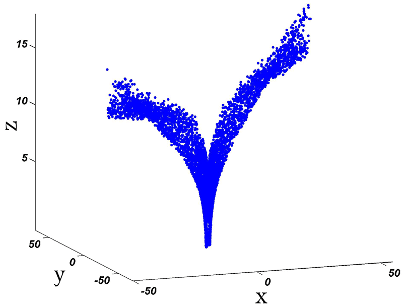
The final position of the protons in the Cartesian and spherical coordinates is shown in figures 3 and 4. As seen, most of the particles are accelerated to distances far away from the non-null point and mostly reach azimuthal angles
 $\unicode[STIX]{x1D719}\sim 45^{\circ }$
and
 $-135^{\circ }$
. Therefore, most of the protons (
 ${\sim}70\,\%$
of the population) are symmetrically distributed close to the bisector line of the first and third quarters of the
 $x{-}y$
plane.
Final position of the particles.

Final position of the particles in spherical coordinates (
 $\unicode[STIX]{x1D719},\unicode[STIX]{x1D703}$
).

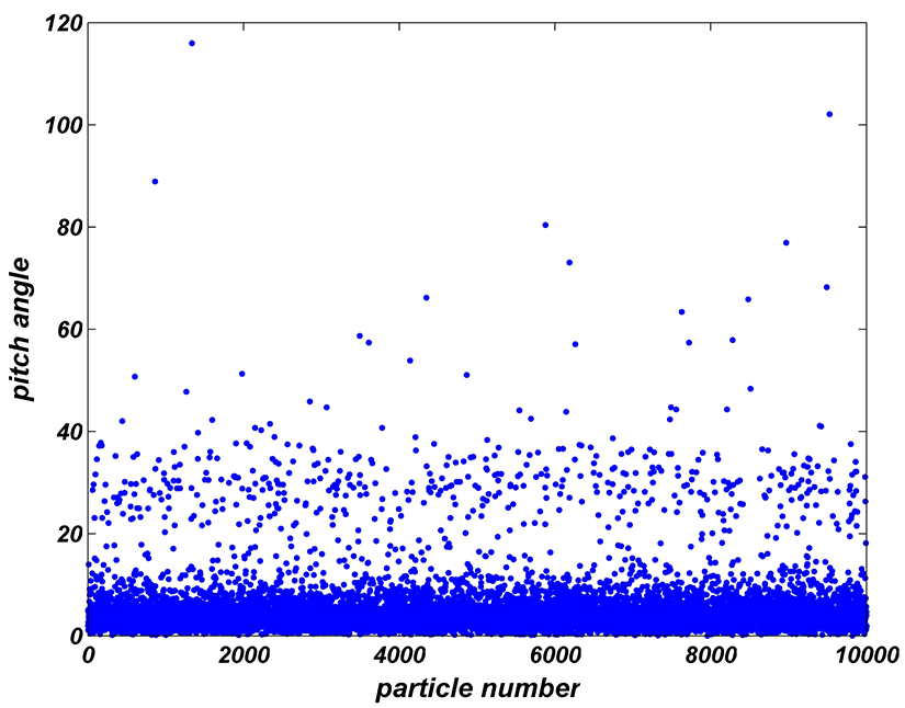
On the other hand, approximately 92 % of the population obtain a pitch angle less than
 $10^{\circ }$
(65 % less than
 $5^{\circ }$
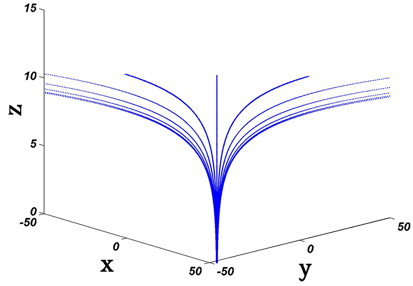
) at the final time (figure 5), indicating that most of the protons follow the direction of the magnetic field lines. The plot of magnetic field lines at larger distances is shown in figure 6.
Final pitch angle of the particles.

Plot of magnetic field lines for equilibrium magnetic field at larger distances.

To find out the reason of such a spatial distribution, we look at the variation of the magnitude of both the electric field and the electric drift velocity,
 $\boldsymbol{V}_{E}=(\boldsymbol{E}\times \boldsymbol{B})/\boldsymbol{B}^{2}$
, in the
 $x{-}y$
plane. Figures 7 and 8 show the contour plots for the magnitudes of the electric field given by (2.8) and the electric drift velocity, respectively. Note that in these figures, contours for very low magnitudes have not been plotted.
Contour plots of the magnitude of the electric field at the
 $x{-}y$
plane.

Contour plots of the magnitude of the electric drift velocity at the
 $x{-}y$
plane.

According to figures 7 and 8, the magnitudes of both the electric field and the electric drift velocity are greater close to the bisector lines of quarters in the
 $x{-}y$
plane. However, the maxima take place at the first and third quarters. Thus, it is expected that a particle injected close to
 $\unicode[STIX]{x1D719}\sim 45^{\circ }$
,
 $-135^{\circ }$
, finally, will be accelerated to a higher energy and so will move a greater distance from the non-null point. Moreover, since the drift velocity is also greater there, the particles finally drift to this regions. Figure 9 plots the initial positions of the injected particles where each point is colour coded according to the final particle energy so we can identify which initial positions will result in what final energy. The kinetic energy of a relativistic particle is calculated as
 $E_{k}=\sqrt{c^{2}p^{2}+m_{0}^{2}c^{4}}-m_{0}c^{2}$
which reduces to
 $E_{k}=1/2m_{0}v^{2}$
in the non-relativistic case. Particles represented by the black colour gain energies less than 100 keV. Blue and green points refer to kinetic energies of
 $100~\text{keV}<E_{k}<10~\text{MeV}$
,
 $10~\text{MeV}<E_{k}<100~\text{MeV}$
, respectively, while red coloured particles represent higher kinetic energies, greater than 100 MeV. As seen, particles injected close to
 $\unicode[STIX]{x1D719}\sim 45^{\circ }$
,
 $-135^{\circ }$
, where the electric field is strongest, obtain the highest kinetic energies. As expected, these particles move to distances farther away from the non-null point.
Initial position of particles (
 $\unicode[STIX]{x1D719}_{0}$
,
 $\unicode[STIX]{x1D703}_{0}$
). Black dots:
 $E_{k}<100~\text{keV}$
; blue dots:
 $100~\text{keV}<E_{k}<10~\text{MeV}$
; green dots:
 $10~\text{MeV}<E_{k}<100~\text{MeV}$
; red dots:
 $E_{k}>100~\text{MeV}$
.

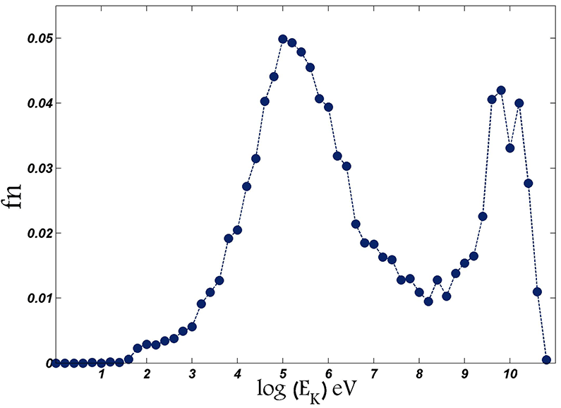
Furthermore, figure 10 shows the energy distribution of the population (the number of the particles in each energy range divided by the total number of particles,
 $fn$
) with
 $b_{0}=0.01T$
and
 $e_{0}=1.0~\text{kV}~\text{m}^{-1}$
. There are two peaks in the plot of energy distribution; the first peak at approximately
 $E_{k}\sim 100~\text{keV}$
and the other at very high energies of
 $E_{k}\sim 10~\text{GeV}$
. These peaks are attributed to acceleration by the strong electric fields around the two bisector lines; the bisector line of the first and third quarters and the bisector line of the second and fourth quarters. Since around the former bisector line the electric field is much stronger, the particles accelerated by this fields reach very high kinetic energies, even of the order of GeV. Production of GeV particles has already been reported in some observational studies. According to Aschwanden (Reference Aschwanden2012), the largest solar energetic particle events accelerate GeV ions with sufficient intensity so that secondary particles are also detected by ground-level facilities. Also, Falcone et al. (Reference Falcone2003), by using Milagrito as an extensive air-shower observatory, have found direct evidence for flux of energetic protons above 4 GeV. Moreover, recently, time profiles of the 0.1–1 GeV protons associated with solar relativistic particle events have been analysed and discussed by Kocharov et al. (Reference Kocharov2015).
Energy distribution of the particles
 $b_{0}=0.01T$
and
 $e_{0}=1.0~\text{kV}~\text{m}^{-1}$
.

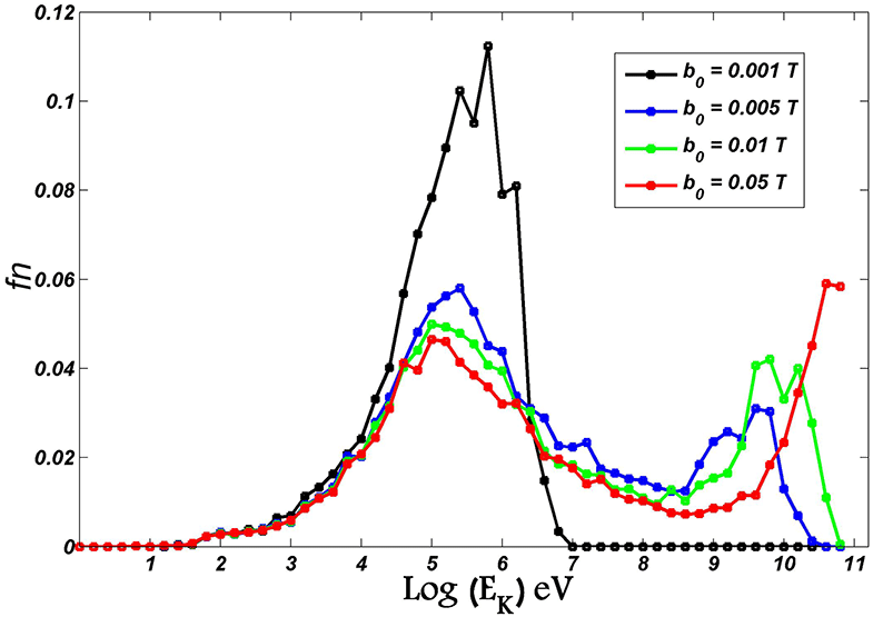
Energy distribution of the particles for different values of
 $b_{0}$
with
 $e_{0}=1.0~\text{kV}~\text{m}^{-1}$
.
The last point to note is that the energy distribution strongly depends on the magnetic and electric field amplitudes
 $b_{0}$
,
 $e_{0}$
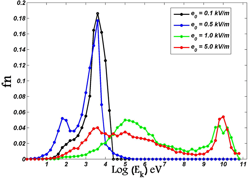
. Figures 11 and 12 plot the variation of energy distribution for different values of
 $b_{0}$
and
 $e_{0}$
. According to figure 11, where
 $e_{0}=1~\text{kV}~\text{m}^{-1}$
, with the smallest value of
 $b_{0}=0.001T$
there is only one peak between 100 keV–1 MeV, however by increasing
 $b_{0}$
, another peak appears at higher values of kinetic energy, which is shifted to very high kinetic energies at larger values of
 $b_{0}$
. Also, by increasing
 $b_{0}$
, a larger portion of the population obtains very high energies, of the order of a few
 $GeV$
. Similarly, according to figure 12, where
 $b_{0}=0.01T$
, with
 $e_{0}=0.1~\text{kV}~\text{m}^{-1}$
there is only one peak between 1 and 10 keV, however, by increasing
 $e_{0}$
, another peak appears at larger values of the energy. The second peak is shifted to higher energies as
 $b_{0}$
increases.
Energy distribution of the particles for different values of
 $e_{0}$
with
 $b_{0}=0.01T$
.

4 Conclusions
By taking into account the static electric and magnetic fields supporting a particular model of stationary non-null magnetic reconnection, we investigated, for the first time, features of the acceleration for a population of 10 000 protons. In this model, a uniform current flowing in only one direction was considered. The injection positions were inside a cubic space around the non-null point and the initial velocities of protons were randomly distributed according to a Maxwellian distribution. Presented results showed that most of the protons are accelerated and move on the bisector line of the first and third quarters in the
 $x{-}y$
plane, i.e.
 $\unicode[STIX]{x1D719}\sim 45^{\circ }$
,
 $-135^{\circ }$
. On this line, the electric field, and so also the electric drift velocity, have their maximum magnitudes. Hence, it is expected that a proton injected close to this line will be accelerated to higher energies. The spatial distribution, however, is not highly collimated in the form of jets, such as the one we found for torsional spine reconnection as a type of null-point reconnection (Hosseinpour Reference Hosseinpour2015). According to our results in non-null reconnection, divergence of the final positions is greater at large distances from the non-null point, similar to the divergence of magnetic field lines.
Furthermore, investigation of the energy distribution showed that with
 $e_{0}=1.0~\text{kV}~\text{m}^{-1}$
and
 $b_{0}=0.01T$
, the average kinetic energy is approximately 2.1 GeV, and therefore most of the particles obtain very high energies. Moreover, by increasing either
 $e_{0}$
or
 $b_{0}$
, two peaks appear in the plot of energy distribution. The second peak takes place at very high kinetic energies, of the order of
 $GeV$
. In our previous works on test particle acceleration with the presence of a null point, namely, torsional spine and fan regimes, (Hosseinpour Reference Hosseinpour2014a
,Reference Hosseinpour
b
, Reference Hosseinpour2015), the final kinetic energy of a proton with similar parameters was only of the order of a few MeV. Comparison of this energy with the average kinetic energy we found here indicates that a non-null model of three-dimensional reconnection is more efficient in accelerating particles to very high kinetic energies, of the order of GeV.
It is worth noting that regarding the number of accelerated particles, the study of Krucker et al. (Reference Krucker2010) reports on the observation of the 2007 DEC 31 Flare, in which the volume of the above-the-loop-top sources is
 $8\times 10^{26}~\text{cm}^{3}$
. This volume is almost
 $10^{11}$
times larger than the one considered in our simulation
 $(10^{15}~\text{cm}^{3})$
. Therefore, if we take into account such a volume, then the number of accelerated particles would be
 $10^{25}\times 10^{11}=10^{36}$
, which is of the same order as reported by Krucker et al. (Reference Krucker2010) and Zharkova et al. (Reference Zharkova, Arzner, Benz, Browning, Dauphin, Emslie, Fletcher, Kontar, Mann and Onofri2011). It also should be noted that we simulate acceleration due to only the magnetic reconnection phenomenon in a small reconnection site, while other acceleration mechanisms can also take part in accelerating particles on larger scales and so increase the number.
The production of accelerated protons with highly relativistic energies is definitely of great significance in explaining the sources of jets and energetic particles in astrophysical contexts, and especially in solar flares. Here we considered a particular model of non-null reconnection where the electric current was simply uniform. A similar analysis can also be extended to the case of a localized current. The authors believe that the results of this study can be of interest for those trying to investigate particle acceleration in more important, dynamic and complex models of non-null reconnection.