1 Introduction
The well-known Taylor–Couette flow (TCF), the flow between two rotating co-axial cylinders, serves as a canonical test bed for studies on hydrodynamic instability, pattern formation, bifurcation theory and the route to chaos (Taylor Reference Taylor1923, Reference Taylor1936a
,Reference Taylor
b
; Chandrasekhar Reference Chandrasekhar1960; Coles Reference Coles1965; Benjamin Reference Benjamin1978a
,Reference Benjamin
b
; Mullin & Benjamin Reference Mullin and Benjamin1980; Benjamin & Mullin Reference Benjamin and Mullin1981; Di Prima & Swinney Reference Di Prima, Swinney, Swinney and Gollub1981; Mullin Reference Mullin1982; Andereck, Liu & Swinney Reference Andereck, Liu and Swinney1986; Chossat & Iooss Reference Chossat and Iooss1994) as well as to understand high-speed turbulence (Grossmann et al.
Reference Grossmann, Lohse and Sun2016) – most of these works are confined to single-phase incompressible Newtonian fluids like water. Andereck et al. (Reference Andereck, Liu and Swinney1986) mapped out a comprehensive phase diagram as a function of the inner- and outer-cylinder Reynolds numbers and characterized numerous flow states via flow-visualization experiments for a Newtonian fluid. For a Newtonian fluid, the TCF, with only the inner cylinder rotating, is centrifugally unstable for any rotation
 $\unicode[STIX]{x1D714}_{i}>0$
according to Rayleigh’s inviscid stability criterion (Rayleigh Reference Rayleigh1916); however, the viscous stability analysis of Taylor (Reference Taylor1923) based on full Navier–Stokes equations (with periodic axial boundary conditions) confirmed a minimum value for the inner-cylinder rotation rate
 $\unicode[STIX]{x1D714}_{i}=\unicode[STIX]{x1D714}_{i}^{min}$
beyond which the purely azimuthal circular Couette flow (CCF) becomes unstable, leading to a stationary pattern of vortices stacked along the axial direction (called Taylor vortex flow, TVF), in excellent agreement with experimental results (Taylor Reference Taylor1936a
,Reference Taylor
b
; Donnelly & Fultz Reference Donnelly and Fultz1960). With further increase in the rotation rate, the stationary Taylor vortices undergo a secondary transition, yielding azimuthally propagating wavy Taylor vortices (WTV); the WTV subsequently giving birth to modulated waves before turbulence sets in.
In addition to numerous studies on the TCF of Newtonian fluids, including those with ‘counter-rotating’ and ‘co-rotating’ cylinders (Coles Reference Coles1965; Andereck et al. Reference Andereck, Liu and Swinney1986), this configuration has also been used as a model system to study flow instabilities in complex fluids due to its simple geometry and the ability to perform controlled experiments. For example, the studies by Larson, Shaqfeh & Muller (Reference Larson, Shaqfeh and Muller1990) uncovered the presence of purely elastic instabilities in Taylor–Couette flow of a dilute polymer solution; Groisman & Steinberg (Reference Groisman and Steinberg1997) observed solitary vortex pairs in Taylor–Couette flow of a highly elastic polymer solution; more recently, Fardin et al. (Reference Fardin, Lasne, Cardoso, Grégoire, Argentina, Decruppe and Lerouge2009) found Taylor-like vortices in a shear-banded flow of worm-like micelles. The above instabilities encountered in complex fluids typically occur at small Reynolds numbers (i.e. the fluid inertia is negligible) and are driven by normal-stress differences and fluid elasticity, and hence they are fundamentally different from well-studied ‘inertial’ instabilities (Taylor Reference Taylor1923; Chandrasekhar Reference Chandrasekhar1960) in Newtonian fluids. This paper deals with inertial instabilities in the Taylor–Couette flow of a non-Brownian Stokesian suspension of neutrally buoyant particles.
Particulate suspensions exhibit migration phenomena when a neutrally buoyant sphere is suspended in a shear flow. This was first observed in pipe Poiseuille flow by Segre & Silberberg (Reference Segre and Silberberg1962) who found that the sphere slowly moves to an equilibrium position at a location 60 % away from the centreline of the pipe. Analysis of the above phenomena using creeping flow approximation showed that this lateral migration was not possible. Later, it was found out theoretically that nonlinear inertial terms in the Navier–Stokes equations contributed to a lateral force due to the stress on the sphere surface (Ho & Leal Reference Ho and Leal1974; Vasseur & Cox Reference Vasseur and Cox1976). Halow & Wills (Reference Halow and Wills1970) observed that neutrally buoyant spheres in a cylindrical Couette geometry migrated to an equilibrium position around the mid-point of the Couette gap. More recently, Majji & Morris (Reference Majji and Morris2018) studied inertial migration of particles in different regimes of a Taylor–Couette system with a particle volume fraction of 0.001 (i.e. in the tracer limit). They found that while the particles are almost homogeneously distributed across the radial–axial plane in the WTV regime, the equilibrium position of particles corresponds to (i) a nearly circular region around each vortex in the TVF regime and (ii) an axial location around the mid-gap towards the inner cylinder in the CCF regime.
While the shear-induced/inertial migration of particles is well understood, the role of particles on inertial instabilities and the transition to turbulence is a relatively unexplored area. The effect of particles on the transition to turbulence in a pipe flow was studied by Matas, Morris & Guazzelli (Reference Matas, Morris and Guazzelli2003) for a wide range of particle loadings. They identified a dual effect of destabilization or stabilization of the flow depending on whether the ratio of the pipe diameter and the particle diameter is smaller, or larger than 65, respectively; while the delayed transition was explained in terms of the enhancement of the effective viscosity of the suspension, the sub-critical transition was thought to be due to the fluctuations triggered by the particles. In a recent experimental work, Majji, Banerjee & Morris (Reference Majji, Banerjee and Morris2018) carried out a set of carefully crafted flow-visualization experiments on inertial transitions in a Taylor–Couette set-up of a neutrally buoyant suspension with the inner cylinder rotating. They showed that the effect of particles is to reduce the critical Reynolds number, implying an early onset of primary instabilities compared to the Newtonian counterparts. For the first time they mapped out a phase diagram between Reynolds number and particle volume fraction, and identified two new states: (i) the spiral vortices and (ii) the ribbons. While the spiral vortices are axially propagating travelling waves, the ribbons (or inter-penetrating spirals, see Andereck et al. (Reference Andereck, Liu and Swinney1986)) represent nonlinear stationary patterns that originate from the interaction between up- and down-propagating spiral vortices. Both these ‘non-axisymmetric’ states were found to be a primary bifurcation from the CCF state of suspension, which are absent in a similar Taylor–Couette set-up with a Newtonian fluid. It may be noted that both spiral vortices and ribbons are known to appear in counter-rotating TCF (Coles Reference Coles1965; Andereck et al.
Reference Andereck, Liu and Swinney1986), as primary bifurcations from the circular Couette flow in the narrow-gap limit. Majji et al. (Reference Majji, Banerjee and Morris2018) presented most of their results for ramp-down experiments (decreasing the inner-cylinder rotation from a high value in a quasi-steady manner) between two different Reynolds numbers; they found that the ramp-up protocol (quasi-steady increase of the inner-cylinder rotation from a minimum value) results in particle accumulation in the core of the Taylor vortices which led to a concentration inhomogeneity. Ideally, both ramp-up and ramp-down experiments should be done to check whether (i) the observed patterns are associated with hysteresis; and/or, (ii) entirely new patterns may crop up during ramp-up experiments. Results presented in figure 10 of Majji et al. (Reference Majji, Banerjee and Morris2018) for a particle volume fraction of
 $\unicode[STIX]{x1D719}=0.1$
suggest that although the pattern transitions remain qualitatively the same during up-sweep and down-sweep experiments, there can be significant hysteresis for both primary and secondary bifurcations.
To better understand the patterns in suspension TCF, further studies are required with different flow conditions and geometric parameters as well as via torque (Taylor Reference Taylor1936a
) and velocity (Taylor Reference Taylor1936b
) measurements. Several questions arise to ascertain the structural characteristics of observed patterns in suspension TCF in terms of the velocity field. How do neutrally buoyant particles influence the structures of Taylor vortices and the related non-axisymmetric travelling patterns? How do particles influence the (i) mean azimuthal velocity and (ii) the fluctuation (radial and axial) kinetic energy in TCF? How does the fluctuation energy change with particle loading? The latter point is important since a prior work (Matas et al.
Reference Matas, Morris and Guazzelli2003) speculated about the possible role of fluctuations triggered by the particles on sub-critical transitions in a particulate pipe flow. These issues can be addressed only via detailed velocity measurements in the radial–axial (
 $r,z$
) and radial–azimuthal (
 $r,\unicode[STIX]{x1D703}$
) planes which constitute one major goal of the present work.
In this work, we carry out experiments to study the flow patterns of a neutrally buoyant non-Brownian suspension in a narrow-gap Taylor–Couette flow system. All experiments are conducted with the inner cylinder rotating and the outer one at rest. Along with flow visualization of the patterns, simultaneous torque measurements are also carried out. In addition, the velocity measurements are performed using particle image velocimetry in both the (
 $r,z$
) and (
 $r,\unicode[STIX]{x1D703}$
) planes. This paper is organized as follows. Experimental details are described in § 2. The critical parameters for both primary and secondary bifurcations on Newtonian TCF are verified in § 3.1 from both flow-visualization studies and torque measurements. In § 3.2, the flow-visualization observations of various patterns in suspension TCF are reported by varying the inner-cylinder Reynolds number (
 $Re$
), particle volume fraction (
 $\unicode[STIX]{x1D719}$
), aspect ratio (
 $\unicode[STIX]{x1D6E4}$
) and radius ratio (
 $\unicode[STIX]{x1D702}$
). Experiments are done in both ramp-up and ramp-down protocols; two novel co-existing states of stationary and travelling waves, found only during ramp-up experiments, are analysed in detail in § 3.2.2 using space–time plots; the similarities and differences with the recent work of Majji et al. (Reference Majji, Banerjee and Morris2018) are highlighted. The effects of varying
 $\unicode[STIX]{x1D6E4}$
and
 $\unicode[STIX]{x1D702}$
on the observed patterns are discussed in § 3.2.3, and the hysteresis for secondary bifurcation is analysed in § 3.2.4. The measurement of wave speeds of both azimuthally and axially propagating travelling waves is described in § 3.2.5. In § 4, the results of PIV (particle image velocimetry) measurements are reported for the velocity field in the radial–axial plane; the Taylor vortices are characterized in terms of their radial and axial velocities for a range of particle volume fractions. In § 5 the structural features and stability of the newly uncovered mixed patterns are analysed in terms of their (
 $r,z$
)-plane streamlines and radial velocities. The characteristics of the radial profiles of the azimuthal velocity are analysed in § 6.1 and the angular-momentum field is discussed in § 6.2 with reference to Rayleigh’s instability criterion. An overall summary of our findings and conclusions, with possible future work, are provided in § 7.
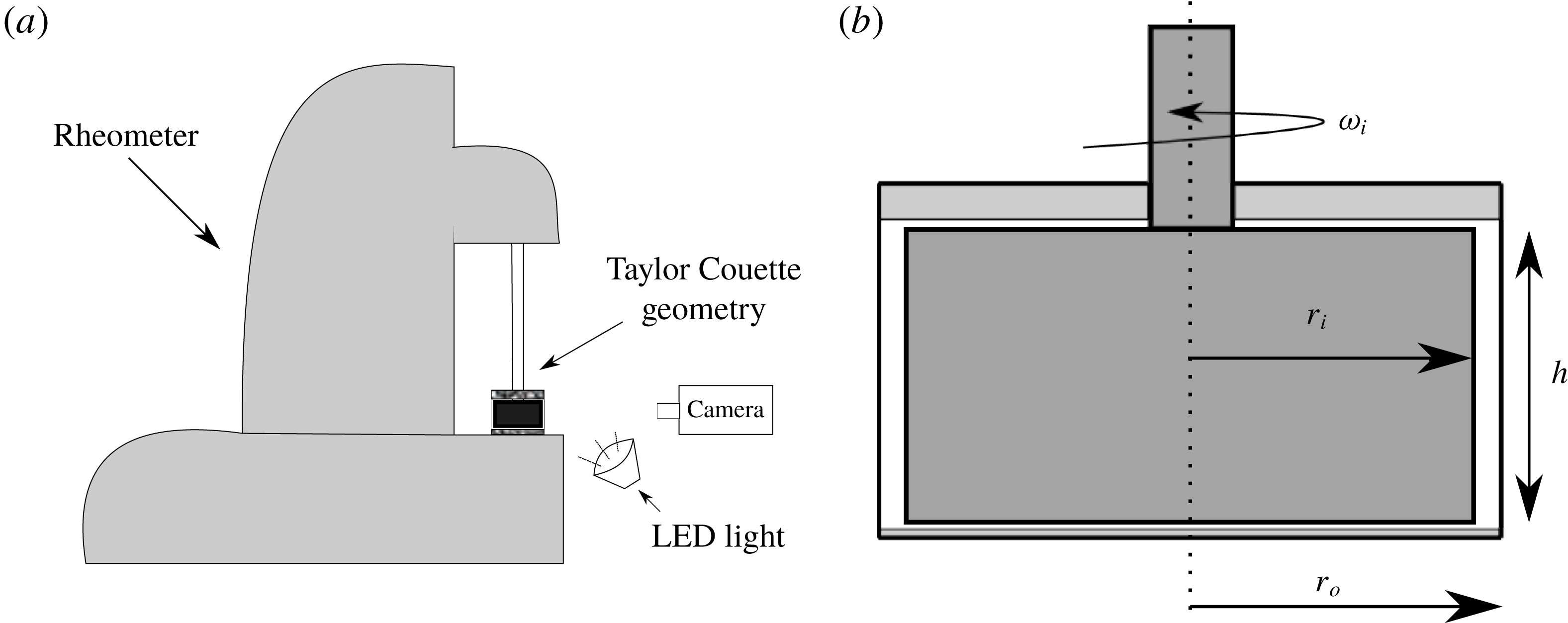
(a) Schematic of Taylor Couette set-up on an Anton-Paar MCR-302 rheometer with end caps for no-slip boundary condition on the top and bottom surfaces. (b) Front view of the Taylor–Couette set-up; there is a small clearance at the top and bottom to facilitate the motion of the inner cylinder.

2 Experimental details
2.1 Taylor–Couette cell and the rheometer
The experimental set-up, shown in figure 1, consists of a pair of concentric cylinders mounted on an Anton-Paar MCR-302 rheometer (which is mounted on an optical table in order to isolate it from external disturbances). The inner cylinder is made of anodized aluminium and is black in colour to minimize reflections. The outer cylinder is made of BK7 glass and is transparent to allow for optical access. The radii of the inner and outer cylinders are
 $r_{i}=16$
mm and
 $r_{o}=17.5$
mm, respectively, yielding a gap width of
 $\unicode[STIX]{x1D6FF}=r_{o}-r_{i}=1.5$
mm and a radius ratio of
 $\unicode[STIX]{x1D702}=r_{i}/r_{o}=0.914$
. The height of the inner cylinder is
 $h=16.5$
mm (as well as the height of the fluid level), which gives an aspect ratio of
 $\unicode[STIX]{x1D6E4}=h/\unicode[STIX]{x1D6FF}=11$
. An annular 3-D printed lid is placed on top of the inner cylinder and a circular disk is placed on the bottom of the inner cylinder to impose no-slip boundary conditions on the top and bottom surfaces. For most of the experiments reported here, the above two geometric parameters are fixed (
 $\unicode[STIX]{x1D6E4}=11$
and
 $\unicode[STIX]{x1D702}=0.914$
), but the protocol to vary
 $\unicode[STIX]{x1D6E4}$
and
 $\unicode[STIX]{x1D702}$
will be discussed in § 3.2.3 to assess the effects of finite values of
 $\unicode[STIX]{x1D6E4}$
and
 $\unicode[STIX]{x1D702}$
on observed patterns.
The inner cylinder is rotated at an angular speed
 $\unicode[STIX]{x1D714}_{i}$
using an electronically commutated motor which is attached to the rheometer. This rheometer allows for precise rotation control which helps in performing both ramp-up (increasing rotation rate
 $\unicode[STIX]{x1D714}_{i}$
) and ramp-down (decreasing rotation rate
 $\unicode[STIX]{x1D714}_{i}$
) experiments as described in § 2.3.
2.2 Neutrally buoyant suspension and its viscosity
The particles used for the suspension are Polymethyl methacrylate (PMMA) micro-spheres with a mean diameter
 $d_{p}=40~\unicode[STIX]{x03BC}\text{m}~(35~\unicode[STIX]{x03BC}\text{m}\leqslant d_{p}\leqslant 45~\unicode[STIX]{x03BC}\text{m})$
, material density
 $\unicode[STIX]{x1D70C}_{p}=1180~\text{kg}~\text{m}^{-3}$
and refractive index
 $n=1.4873$
. This yields a gap to particle size ratio of
 $\unicode[STIX]{x1D6FF}/d_{p}=37.5$
. A density- and refractive-index-matched solvent was prepared using the recipe suggested by Bailey & Yoda (Reference Bailey and Yoda2003) which consists of a ternary mixture of water (29.5 %), glycerine (34.3 %) and ammonium thiocyanate
 $\text{NH}_{4}\text{SCN}$
(36.2 %) by volume, yielding a solvent with effective density
 $\unicode[STIX]{x1D70C}=1182.16~\text{kg}~\text{m}^{-3}\approx \unicode[STIX]{x1D70C}_{p}$
, refractive index
 $n=1.4884$
and shear viscosity
 $\unicode[STIX]{x1D707}_{l}=6.846~\text{mPa}~\text{s}$
at
 $T=22\,^{\circ }$
C. The density of the solvent was measured using a density meter (Rudolph: DDM-2909).
The suspension is prepared at various values of particle volume fraction,
 $$\begin{eqnarray}\displaystyle \unicode[STIX]{x1D719}=\frac{\unicode[STIX]{x03C0}d_{p}^{3}N}{6V}, & & \displaystyle\end{eqnarray}$$
where
 $N$
is the total number of particles and
 $V$
is the volume of the annular cell. The shear viscosity of the suspension is measured separately using a parallel-plate geometry in the same Anton-Paar MCR-302 rheometer with a plate diameter of 50 mm and a gap of 0.8 mm. We have verified that the average suspension viscosity data (not shown) closely follow the Krieger–Dougherty relation,
 $$\begin{eqnarray}\displaystyle \unicode[STIX]{x1D707}=\unicode[STIX]{x1D707}_{l}\left(1-\frac{\unicode[STIX]{x1D719}}{\unicode[STIX]{x1D719}_{m}}\right)^{-\unicode[STIX]{x1D6FD}}, & & \displaystyle\end{eqnarray}$$
with exponents given by (i)
 $(\unicode[STIX]{x1D6FD},\unicode[STIX]{x1D719}_{m})=(1.8,0.55)$
and (ii)
 $(\unicode[STIX]{x1D6FD},\unicode[STIX]{x1D719}_{m})=(2,0.585)$
. The normal-stress differences were also measured (not shown) using the cone-plate and parallel-plate configurations in the same rheometer. We found that both first and second normal-stress differences are negative but negligible at
 $\unicode[STIX]{x1D719}\leqslant 0.15$
, and both increase in magnitude with increasing
 $\unicode[STIX]{x1D719}$
at
 $\unicode[STIX]{x1D719}\geqslant 0.2$
; our data closely follow the measured values reported on Stokesian suspensions (see the review article of Guazzelli & Pouliquen (Reference Guazzelli and Pouliquen2018)).
The Reynolds number of the flow, based on the rotational speed of the inner cylinder (
 $\unicode[STIX]{x1D714}_{i}r_{i}$
) and the gap width (
 $\unicode[STIX]{x1D6FF}=r_{o}-r_{i}$
) as the length scale, is defined as
 $$\begin{eqnarray}\displaystyle Re=\frac{\unicode[STIX]{x1D70C}\unicode[STIX]{x1D714}_{i}r_{i}\unicode[STIX]{x1D6FF}}{\unicode[STIX]{x1D707}}, & & \displaystyle\end{eqnarray}$$
where
 $\unicode[STIX]{x1D707}$
is the suspension viscosity (2.2). In the present set-up, we could access a range of Reynolds numbers up to
 $Re\leqslant 200$
.
The particle Reynolds number is
 $Re_{p}=\unicode[STIX]{x1D70C}\dot{\unicode[STIX]{x1D6FE}}{d_{p}}^{2}/4\unicode[STIX]{x1D707}_{l}\sim O(10^{-5})$
, the Stokes number is
 $St=m_{p}\dot{\unicode[STIX]{x1D6FE}}/3\unicode[STIX]{x03C0}\unicode[STIX]{x1D707}_{l}d_{p}\sim O(10^{-4})$
and the Péclet number is
 $Pe=3\unicode[STIX]{x03C0}\unicode[STIX]{x1D707}d^{3}\dot{\unicode[STIX]{x1D6FE}}/4k_{B}T\sim O(10^{8})$
for the range of shear rates (Blanc, Peters & Lemaire Reference Blanc, Peters and Lemaire2011),
 $$\begin{eqnarray}\displaystyle \dot{\unicode[STIX]{x1D6FE}}(r)=2\unicode[STIX]{x1D714}_{i}\frac{r_{i}^{2}r_{o}^{2}}{r_{o}^{2}-r_{i}^{2}}\frac{1}{r^{2}}, & & \displaystyle\end{eqnarray}$$
accessed in the present experiments. This implies that the particles are non-Brownian (
 $Pe\gg 1$
), the inertia of the particles is negligible (
 $Re_{p}\ll 1$
) and the fluid–particle interactions are strong (
 $St\ll 1$
). Therefore, the observed flow phenomena in our suspension TCF are largely driven by fluid inertia (2.3) and it is in this regard that the present experiments are similar to those of Majji et al. (Reference Majji, Banerjee and Morris2018).
2.3 Experimental protocols: flow visualization and torque measurements
The annular gap of the TC cell is filled with a well-mixed suspension of specified particle volume fraction
 $\unicode[STIX]{x1D719}$
. Experiments are started by rotating the inner cylinder, at an angular speed
 $\unicode[STIX]{x1D714}_{i}$
, which is tied to the rheometer and is controlled by a precision motor having a maximum angular frequency of 20 Hz. The temperature is controlled at
 $22\pm 0.01\,^{\circ }\text{C}$
using a water jacket flowing through an additional glass jacket around the outer cylinder.
The experiments are conducted using both ramp-up (increasing rotation speed from
 $\unicode[STIX]{x1D714}_{i}=\unicode[STIX]{x1D714}^{min}$
) and ramp-down (decreasing rotation speed from
 $\unicode[STIX]{x1D714}_{i}=\unicode[STIX]{x1D714}^{max}$
) protocols in a quasi-steady manner, with a ramping rate of
 $\text{d}Re/\text{d}\unicode[STIX]{x1D70F}_{d}\ll 1$
(where
 $Re\sim \unicode[STIX]{x1D714}_{i}$
and
 $\unicode[STIX]{x1D70F}_{d}=t/t_{d}$
is the dimensionless time, with
 $t_{d}=\unicode[STIX]{x1D70C}\unicode[STIX]{x1D6FF}^{2}/\unicode[STIX]{x1D707}$
being the diffusion time scale) between two Reynolds numbers to ensure no effects of acceleration/deceleration (Dutcher & Muller Reference Dutcher and Muller2009). The ramp-up and ramp-down protocols help to identify hysteresis effects during the onset of any flow transition.
Flow is visualized using anisotropic green mica flakes with the largest dimension of
 $35~\unicode[STIX]{x03BC}\text{m}$
and smaller dimensions in the perpendicular directions; typical seeding level is 0.14 % by volume; a 5 W LED lamp is used for illumination. A Nikon-D750 DSLR camera is used to capture images at regular intervals as well as to take videos at 60 fps; the camera is fitted with a 105 mm Nikkor Macro-lens and a polarizer. Images are analysed to construct the ‘space–time’ or ‘space–
 $Re$
’ diagrams of the patterns. Along with flow visualization studies on pattern transitions, the torque measurements are carried out simultaneously using the same rheometer.
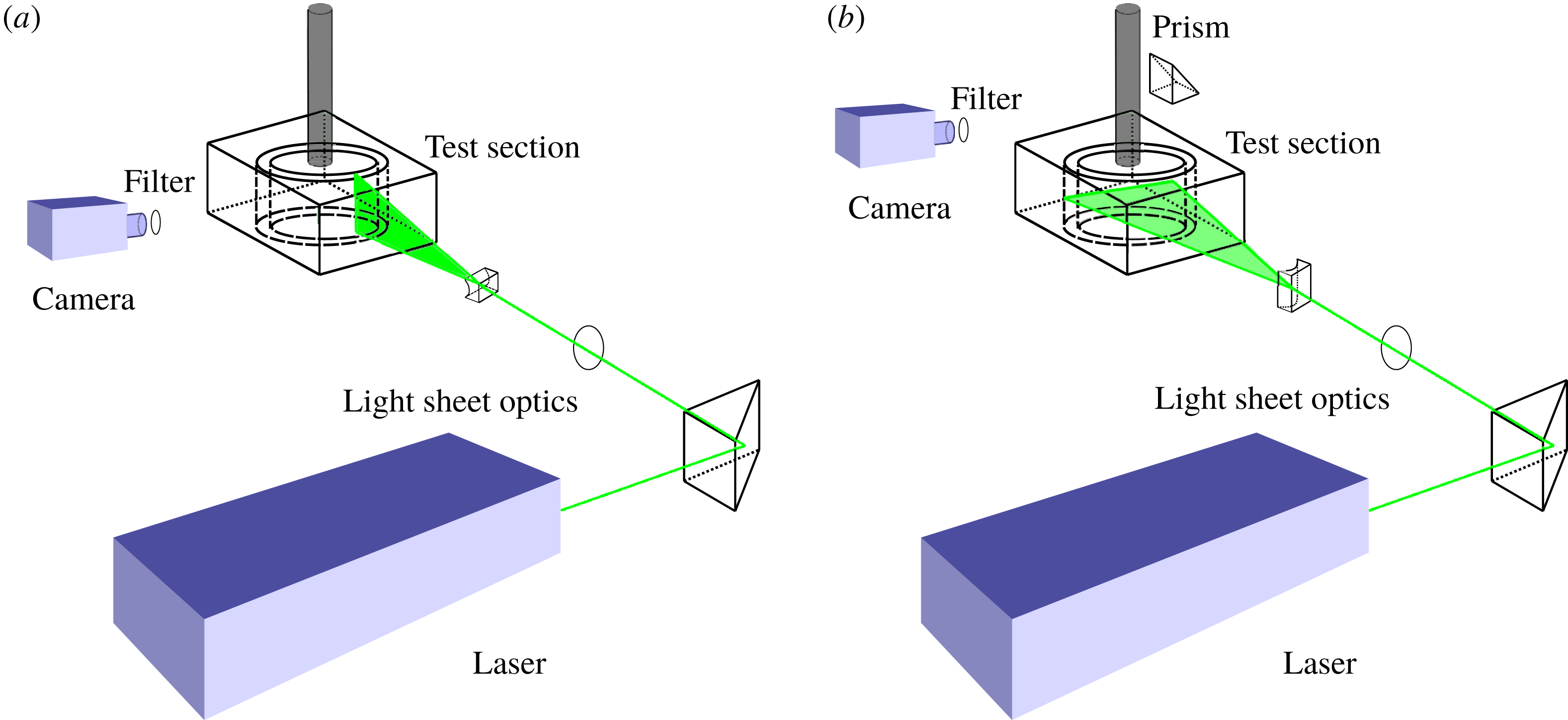
Schematics of the optical configuration for PIV measurements in the (a) gradient–vorticity (
 $r,z$
) plane and (b) flow–gradient (
 $r,\unicode[STIX]{x1D703}$
) plane. Note that an acrylic square box is placed around the cylindrical Taylor–Couette cell to eliminate optical distortions; see the text in § 2.4 for details.

2.4 Velocity measurements with particle image velocimetry
Particle image velocimetry (PIV) has been employed to measure velocity in the gradient–vorticity (
 $r,z$
) plane and the flow–gradient (
 $r,\unicode[STIX]{x1D703}$
) plane at mid-height (
 $h/2$
), as shown schematically in figure 2(a,b). A prism arrangement, as shown in figure 2(b), is made to capture images for PIV measurements in the flow–gradient (
 $r,\unicode[STIX]{x1D703}$
) plane. An acrylic outer cylinder (of radius
 $r_{o}=17.5$
mm and refractive index
 $n\approx 1.49$
) with an acrylic square box (
 $n\approx 1.49$
) around it is used with the Newtonian carrier fluid (
 $n=1.4884$
) filled in between. This led to refractive-index matching which is not possible with a glass (
 $n=1.53$
) outer cylinder. The square outer box has helped in minimizing refraction due to the curved surface of the outer cylinder. For velocity measurements, active temperature control is not possible in the modified system; however, the measurements are made at a room temperature of
 $22\,^{\circ }\text{C}$
, which is maintained constant to within
 $\pm 0.5\,^{\circ }\text{C}$
during each run. Following the procedure of Wereley & Lueptow (Reference Wereley and Lueptow1998) and Tokgoz et al. (Reference Tokgoz, Elsinga, Delfos and Westerweel2012), the fluid and ambient temperatures are monitored before and after each experiment. The temperature of the suspension did not vary by
 $\pm 0.2\,^{\circ }\text{C}$
during the experiment as the measurements were done at low Reynolds numbers. The viscosity of the working fluid is measured before and after the experiment and an uncertainty of 0.6 % was observed.
Fluorescent seeding particles (Cospheric: FMR-1.3) of effective diameter
 $d_{seed}=3~\unicode[STIX]{x03BC}\text{m}~(1~\unicode[STIX]{x03BC}\text{m}\leqslant d_{seed}\leqslant 5~\unicode[STIX]{x03BC}\text{m})$
(emission wavelength
 $=$
607 nm) and density
 $1.3~\text{g}~\text{cm}^{-3}$
were used as tracer particles for PIV measurements with a long-pass filter (550 nm) to eliminate laser (532 nm) reflections. The Péclet number for seeding particles is
 $$\begin{eqnarray}\displaystyle Pe_{seed}=\frac{3\unicode[STIX]{x03C0}\unicode[STIX]{x1D707}\,d_{seed}^{3}\,\dot{\unicode[STIX]{x1D6FE}}}{4k_{B}T}\sim O(10^{5}), & & \displaystyle\end{eqnarray}$$
and hence the Brownian motion of seeding particles can be neglected (Blanc et al. Reference Blanc, Peters and Lemaire2011).
A dual-head 532 nm Nd-YAG Litron laser (Litron Bernoulli laser series, 200 mJ/pulse, 15 Hz) is used for illumination, and the time between paired laser pulses is varied
 $\unicode[STIX]{x0394}t\in (80,500)~\unicode[STIX]{x03BC}\text{s}$
; the laser sheet thickness is approximately 1 mm. A CCD camera (Dantec Dynamics FlowSense, Model number: EO 16M-9) with a resolution of
 $4896\times 3264$
pixels (i.e.
 $16$
megapixel with pixel size of
 $5.5~\unicode[STIX]{x03BC}\text{m}$
and an inter-frame time limit of 200 ns) is synchronized with the laser to acquire double-frame images at 4.454 Hz. For each PIV measurement, 500 image pairs are acquired which are subsequently analysed using the adaptive-correlation technique of the ‘Dynamic-Studio’ software (of Dantec Dynamics A/S, Denmark, Version 6.2); an interrogation window of
 $32\times 32$
pixels with 75 % overlap is used for this analysis.
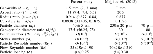
A comparison of geometric parameters and various non-dimensional numbers between the present work and Majji et al. (Reference Majji, Banerjee and Morris2018). For both studies, the system has dominant fluid inertia (
 $Re\gg 1$
), but the particle inertia (
 $Re_{p}\ll 1$
) is negligible and the fluid–particle coupling (
 $St\ll 1$
) is strong (representing non-Brownian viscous suspension).

3 Pattern transition and phase diagram
Most of the present experiments were performed with a radius ratio of
 $\unicode[STIX]{x1D702}=0.914$
and an aspect ratio of
 $\unicode[STIX]{x1D6E4}=11$
, with a rigid lid at the top of the Taylor–Couette cell. The effects of changing
 $\unicode[STIX]{x1D6E4}$
and
 $\unicode[STIX]{x1D702}$
on observed patterns were checked for a few cases (as well as with a free surface boundary condition at the top) as discussed in § 3.2.3. Table 1 indicates that the geometric parameters and various dimensionless numbers in the present set-up are of comparable magnitudes to those of Majji et al. (Reference Majji, Banerjee and Morris2018). For both studies, the system has dominant fluid inertia (
 $Re\gg 1$
), but the particle inertia (
 $Re_{p}\ll 1$
) is negligible and the fluid–particle coupling (
 $St\ll 1$
) is strong. In § 3.1 we briefly discuss different patterns in the TCF of a Newtonian fluid, followed by present results on suspension TCF in § 3.2.
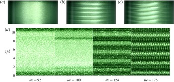
Snapshots of patterns in TCF of a Newtonian fluid at (a)
 $Re=92$
(circular Couette flow, CCF), (b)
 $Re=124$
(Taylor vortex flow, TVF) and (c)
 $Re=176$
(wavy Taylor vortex, WTV). (d) Space–time evolution of patterns: CCF (
 $Re=92$
), Ekman vortices with CCF (
 $Re=100$
), TVF (
 $Re=124$
) and WTV (
 $Re=176$
). The ramping rate is
 $\text{d}Re/\text{d}\unicode[STIX]{x1D70F}_{d}=0.027$
.

3.1 Taylor–Couette flow of a Newtonian fluid
For the Newtonian solvent (§ 2.2), the experiments were carried out in both ramp-up and ramp-down protocols with Reynolds numbers of
 $Re=90$
to
 $Re=190$
at a ramping rate of
 $\text{d}Re/\text{d}\unicode[STIX]{x1D70F}_{d}=0.027$
. Figure 3(a–c) displays typical snapshots of three distinct patterns with increasing Reynolds number; figure 3(d) displays the temporal evolution of these patterns at four values of
 $Re$
, each developed over a time span of 2 s. Note the emergence of two Ekman vortices near the end walls in the first (
 $Re=92$
) and second (
 $Re=100$
) images of figure 3(d) – the origin of such Ekman vortices (Coles Reference Coles1965; Cole Reference Cole1976) is tied to the no-slip boundary condition at the top and bottom rigid lids of finite-size Taylor–Couette cells. In any case, the ‘bulk’ flow at sub-critical Reynolds numbers such as in figure 3(a) appears to be purely azimuthal [
 $v_{\unicode[STIX]{x1D703}}(r)\neq 0$
,
 $v_{r}=0=v_{z}$
], except near the top and bottom lids – this is called CCF (circular Couette flow), which, with further increasing
 $Re$
, gives birth to an axial array of stationary Taylor vortices, see figure 3(b), called TVF (Taylor vortex flow). The stationarity of TVF is evident from the space–time diagram in the third image in figure 3(d) that corresponds to
 $Re=124$
. As
 $Re$
is increased further, the TVF becomes unstable, giving birth to wavy Taylor vortices (WTV), see figure 3(c), which are travelling waves propagating along the azimuthal direction. From the ‘space–
 $Re$
’ diagram (not shown), we find that the primary transition from CCF to TVF occurs at a critical Reynolds number of
 $Re_{c}\approx 122$
and the secondary bifurcation of TVF
 $\rightarrow$
WTV at
 $Re\approx 170$
.

Along with flow visualization, we have carried out torque measurements using the same rheometer that helped to identify the onset of primary bifurcation CCF
 $\rightarrow$
TVF. The variation of the dimensionless torque on the inner cylinder (Martínez-Arias et al.
Reference Martínez-Arias, Peixinho, Crumeyrolle and Mutabazi2014),
 $$\begin{eqnarray}\displaystyle G=\frac{{\mathcal{T}}}{2\unicode[STIX]{x03C0}\unicode[STIX]{x1D707}^{2}h/\unicode[STIX]{x1D70C}}, & & \displaystyle\end{eqnarray}$$
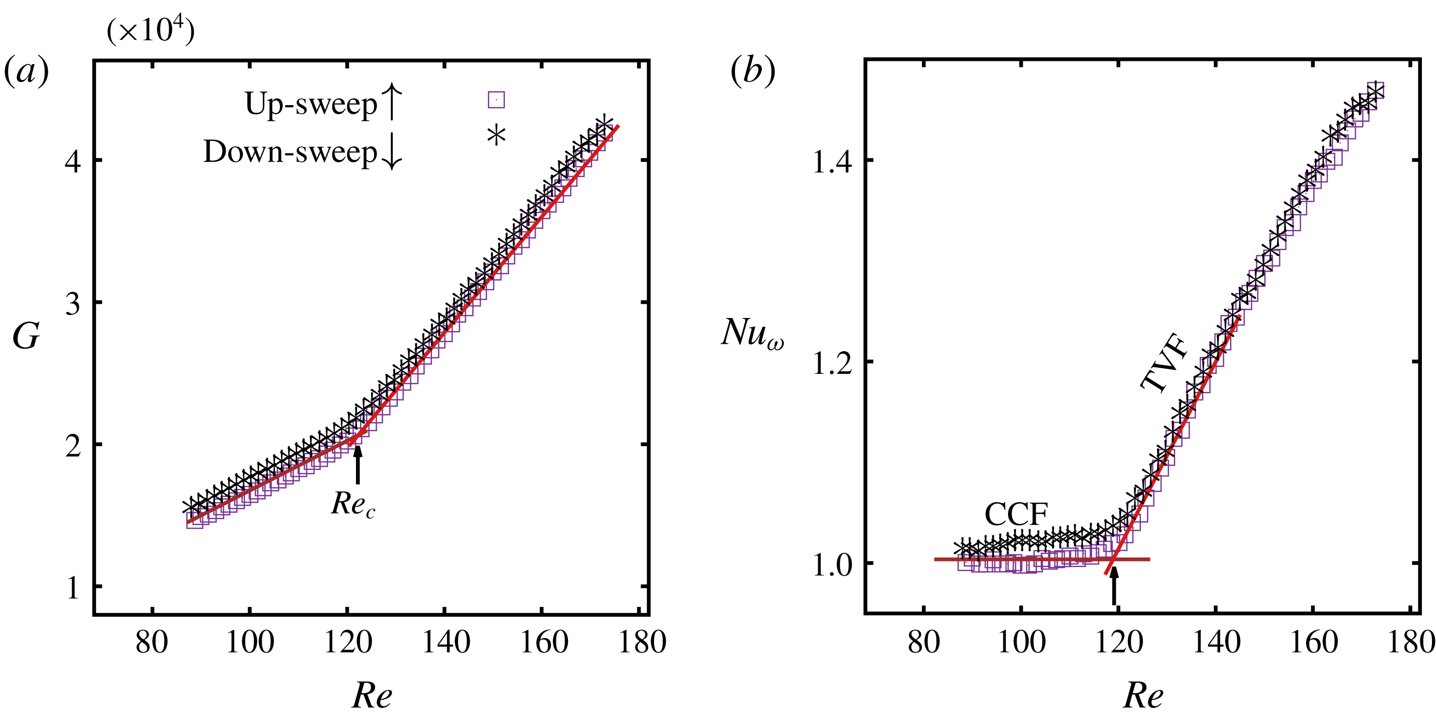
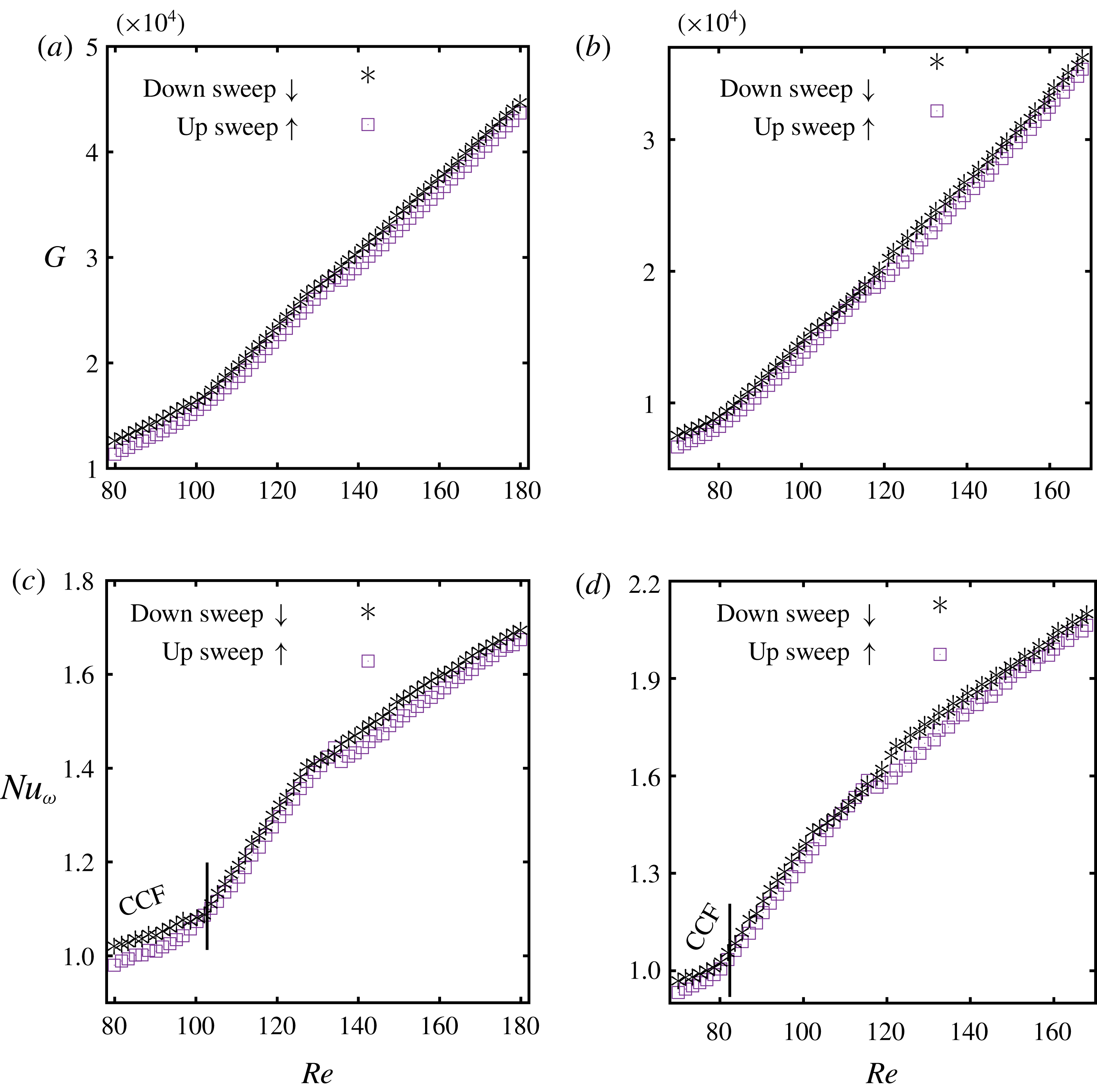
with Reynolds number is shown in figure 4(a) as measured during up-sweep (denoted by squares) and down-sweep (stars) protocols. For both cases, there is a clear change in the slope of the ‘torque–
 $Re$
’ curve around
 $Re=120$
as the flow makes a transition from CCF to TVF and vice versa. This transition becomes clearer in figure 4(b) which displays the
 $Re$
-variation of the effective Nusselt number (Eckhardt, Grossmann & Lohse Reference Eckhardt, Grossmann and Lohse2007)
 $$\begin{eqnarray}\displaystyle Nu_{\unicode[STIX]{x1D714}}=\frac{G}{G_{0}},\quad \text{where}~G_{0}=\frac{2\unicode[STIX]{x1D702}Re}{(1+\unicode[STIX]{x1D702})(1-\unicode[STIX]{x1D702})^{2}} & & \displaystyle\end{eqnarray}$$
is the laminar torque that holds in the CCF regime of the narrow-gap TCF with infinite cylinders. The ‘
 $Nu_{w}-Re$
’ plot in figure 4(b) confirms a continuous transition from
 $Nu_{w}=1$
(CCF) to
 $Nu_{w}\propto Re$
(TVF); the intersection of above two scaling relations occurs at
 $Re_{c}\approx 120$
which is close to the critical Reynolds number
 $Re_{c}\approx 122$
determined from the ‘space–
 $Re$
’ diagram of the image analysis. It must be noted that the secondary transition from TVF to WTV that occurs at
 $Re\approx 170$
has no discernible signature either in the torque–
 $Re$
curve (figure 4
a), or, in the
 $Nu_{w}-Re$
plot (figure 4
b).
Comparison of critical Reynolds numbers in Newtonian TCF. While Cole’s (Reference Cole1976) data are extrapolated for the present set-up of
 $\unicode[STIX]{x1D6E4}=11$
and
 $\unicode[STIX]{x1D702}=0.914$
, the theoretical values of Di Prima & Swinney (Reference Di Prima, Swinney, Swinney and Gollub1981) correspond to axially periodic boundary conditions (i.e.
 $\unicode[STIX]{x1D6E4}\rightarrow \infty$
).

For the present set-up with
 $\unicode[STIX]{x1D6E4}=11$
and
 $\unicode[STIX]{x1D702}=0.914$
, the experimental data of Cole (Reference Cole1976) can be extrapolated to obtain
 $Re_{c}=129.7$
for CCF
 $\rightarrow$
TVF, and
 $Re_{c}=173.4$
for TVF
 $\rightarrow$
WTV. These values are very close to our findings, see table 2. According to Cole (Reference Cole1976), for
 $\unicode[STIX]{x1D6E4}\leqslant 20$
the transition to TVF occurs at a lower
 $Re$
because of perturbations by end wall/Ekman vortices, and the transition to WTV occurs at a higher
 $Re$
since the waviness of Taylor vortices is delayed due to the stabilization offered by the end wall boundary layers; these two observations are also confirmed in table 2 that also compares the present data with the theoretical stability results of Di Prima & Swinney (Reference Di Prima, Swinney, Swinney and Gollub1981) for TCF with periodic boundary conditions. In summary, our Taylor–Couette set-up can quantitatively reproduce critical Reynolds numbers (Cole Reference Cole1976) for both primary (
 $\text{CCF}\rightarrow \text{TVF}$
) and secondary (
 $\text{TVF}\rightarrow \text{WTV}$
) bifurcations.
Before presenting results on suspension TCF, we would like to point out that the effect of the finite length of the cylinders on the nature of the primary bifurcation has not been quantified in this work – from the torque data in figure 4 (as well as in the Appendix), the primary bifurcation appears to be smooth for both Newtonian and suspension TCF. In this regard, it may be noted that the seminal works of Benjamin, Mullin and co-workers (Benjamin Reference Benjamin1978a
,Reference Benjamin
b
; Benjamin & Mullin Reference Benjamin and Mullin1981; Mullin Reference Mullin1982; Cliffe & Mullin Reference Cliffe and Mullin1985; Cliffe, Mullin & Schaeffer Reference Cliffe, Mullin and Schaeffer2012; Mullin, Heise & Pfister Reference Mullin, Heise and Pfister2017) have revealed that the primary bifurcation in ‘finite-length’ TC cells is very complicated and can occur via saddle-node bifurcations, leading to the multiplicity of states and the anomalous Taylor vortices (Benjamin & Mullin Reference Benjamin and Mullin1981); moreover, the secondary bifurcation from TVF to WTV can result in the appearance of novel singly, multiply or quasi-periodic oscillatory modes (Mullin & Benjamin Reference Mullin and Benjamin1980; Park Reference Park1984; Jones Reference Jones1985; Mullin Reference Mullin1985) depending on the aspect ratio
 $\unicode[STIX]{x1D6E4}$
and
 $Re$
. Tracking the anomalous modes (Benjamin & Mullin Reference Benjamin and Mullin1981) would require an experimental set-up in which
 $\unicode[STIX]{x1D6E4}$
can be changed quasi-statically in a controlled fashion, which is beyond the scope of the present work. For the range of Reynolds numbers
 $Re\leqslant 200$
studied in the present experiments, we did not observe the ‘jet-instability’ mode (Mullin & Benjamin Reference Mullin and Benjamin1980) in our set-up for Newtonian TCF, however, we uncovered two new co-existing states of stationary and travelling Taylor vortices that are reported in § 3.2 – the latter states will be characterized and contrasted with related findings of Mullin (Reference Mullin1985) in § 5.
3.2 Suspension Taylor–Couette flow: phase diagram and co-existing patterns
Moving to the Taylor–Couette flow of neutrally buoyant suspensions, the experiments are carried out for a range of particle volume fractions of
 $\unicode[STIX]{x1D719}=0.01$
, 0.03, 0.05, 0.10, 0.11, 0.12, 0.13, 0.15, 0.20 and 0.25; both ramp-up and ramp-down protocols, at a specified ramping rate
 $\text{d}Re/\text{d}\unicode[STIX]{x1D70F}_{d}\ll 1$
, are employed in all experiments. It must be noted that most of the results represented in this section (except in § 3.2.4) are based on separate/independent runs with ramp-up and ramp-down protocols: each experiment is started with a freshly prepared homogeneous suspension in the TC cell, with the rotation rate being (i) increased from
 $\unicode[STIX]{x1D714}_{i}=\unicode[STIX]{x1D714}_{i}^{min}$
(up-sweep) or (ii) decreased from
 $\unicode[STIX]{x1D714}_{i}=\unicode[STIX]{x1D714}_{i}^{max}$
(down-sweep) linearly at a specified ramping rate from; for both cases the rotation rate is quickly taken to the desired starting value. Torque measurements are also carried out simultaneously that help to identify the onset of primary transition (from the CCF to non-azimuthal flows) accurately. In addition to the well-known patterns (TVF and WTV) of Newtonian TCF, we shall describe non-axisymmetric patterns like the spiral vortex flow (SVF, see Majji et al. (Reference Majji, Banerjee and Morris2018)) as seen in ramp-down experiments as well as two new patterns, uncovered in the ramp-up experiments.
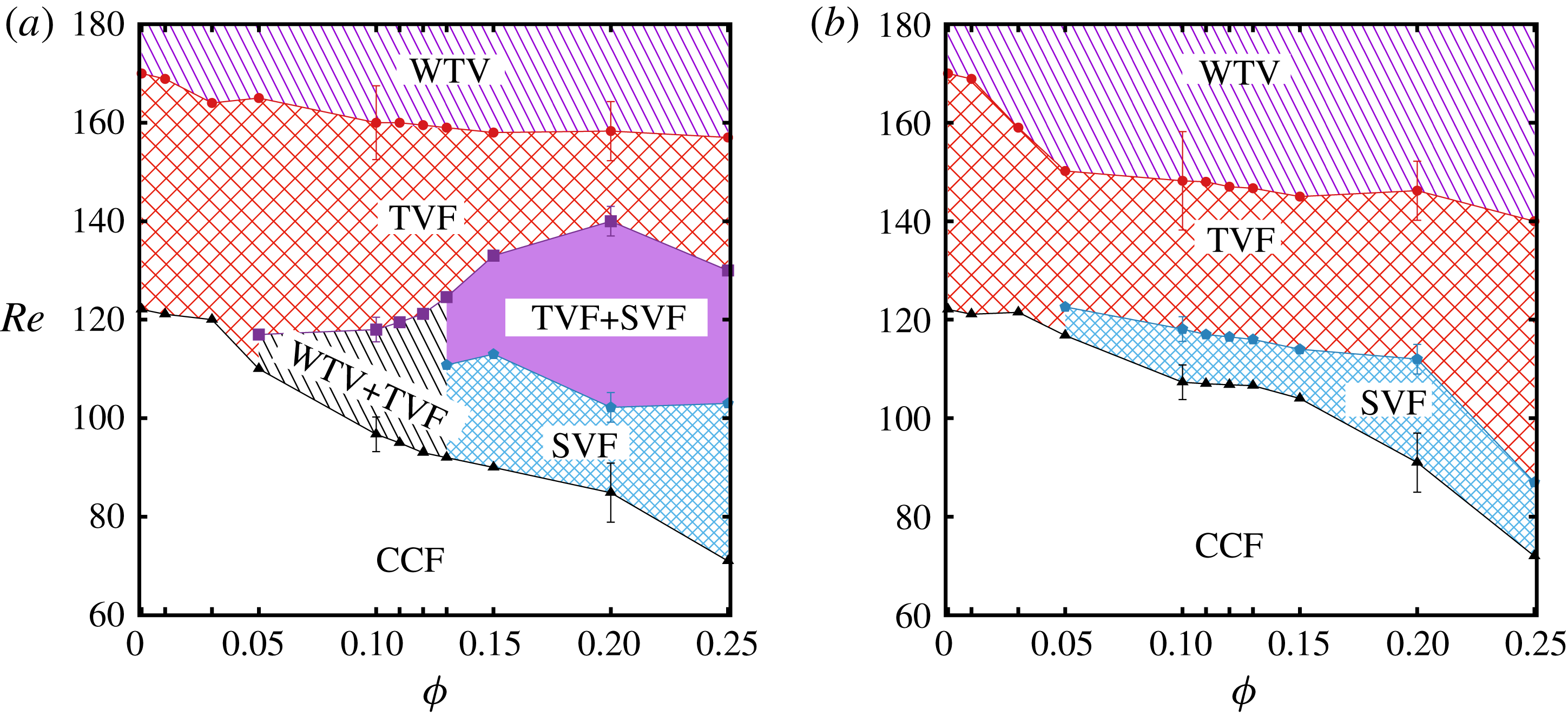
Phase diagrams of patterns in the
 $(Re,\unicode[STIX]{x1D719})$
plane for (a) up-sweep (ramp-up) and (b) down-sweep (ramp-down) experiments. Acronyms for different patterns are as follows: CCF (circular Couette flow), TVF (Taylor vortex flow), WTV (wavy Taylor vortex) and SVF (spiral vortex flow). The error bars at
 $\unicode[STIX]{x1D719}=0.1$
and 0.2 are representative of the maximum variation among three different runs for each experimental protocol.

3.2.1 Phase diagram and the comparison for primary transition
From the movies of quasi-steady ramp-up and ramp-down experiments, the ‘space–
 $Re$
’ plots are constructed that are subsequently used to identify transition from one state to another. Observed patterns are mapped onto a phase diagram in the Reynolds number (
 $Re$
) and particle volume fraction (
 $\unicode[STIX]{x1D719}$
) plane, see figure 5 – while panel (a) corresponds to patterns seen in ramp-up experiments, panel (b) corresponds to its ramp-down counterpart. Note that the up-sweep phase diagram shows more number of patterns compared to the down-sweep phase diagram. For a very dilute suspension with
 $\unicode[STIX]{x1D719}\leqslant 0.03$
, the flow transitions correspond to
 $\text{CCF}\rightarrow \text{TVF}\rightarrow \text{WTV}$
as in the Newtonian TCF, with a slight reduction in the critical
 $Re$
for both
 $\text{CCF}\rightarrow \text{TVF}$
and
 $\text{TVF}\rightarrow \text{WTV}$
transitions as compared to the Newtonian case. At higher particle loadings
 $\unicode[STIX]{x1D719}\geqslant 0.05$
, however, the critical Reynolds number for circular Couette flow to become unstable decreases sharply, with the emergence of new patterns, along with hysteresis, as discussed in § 3.2.2.
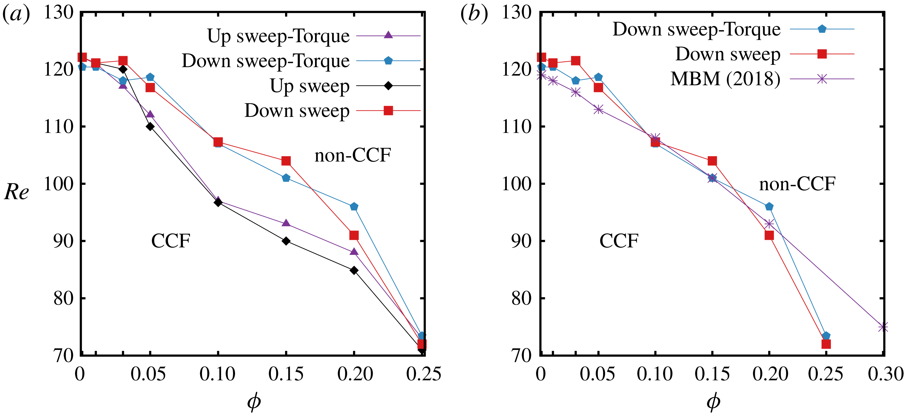
Figure 6(a) shows a comparison of critical
 $Re$
for the primary transition from CCF to other flow states obtained from (i) the image analysis as discussed above (space–
 $Re$
diagram and visual inspection) and (ii) the torque data procured simultaneously from the rheometer. It is seen that there is a close agreement between the image analysis and the torque data for both up-sweep and down-sweep protocols. Figure 6(b) shows a comparison of our critical
 $Re$
with the corresponding data extracted from the phase diagram of Majji et al. (Reference Majji, Banerjee and Morris2018) – both data sets refer to down-sweep protocols. Overall, our data on primary transition agree with the experiments of Majji et al. (Reference Majji, Banerjee and Morris2018), even though the geometrical parameters of two Taylor Couette set-ups differ in terms of both aspect ratio (
 $\unicode[STIX]{x1D6E4}=11$
versus
 $\unicode[STIX]{x1D6E4}_{M}=20.5$
) and radius ratio (
 $\unicode[STIX]{x1D702}=0.914$
versus
 $\unicode[STIX]{x1D702}_{M}=0.877$
). Note in figure 6(b) that there is a sharp decrease in
 $Re_{c}$
beyond
 $\unicode[STIX]{x1D719}=0.2$
as confirmed from both image analysis and torque data.
(a) Comparison of critical
 $Re$
for primary flow transition from CCF to different flow states obtained from space–
 $Re$
diagram and the torque data. (b) Comparison of our down-sweep data on
 $Re_{c}$
with those of Majji et al. (Reference Majji, Banerjee and Morris2018), marked by the starred line.

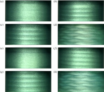
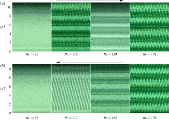
Snapshots of patterns in suspension TCF for
 $\unicode[STIX]{x1D719}=0.10$
. (a)
 $Re=85$
(CCF), (b)
 $Re=115$
(‘WTV
 $+$
TVF’), (c)
 $Re=130$
(TVF), (d)
 $Re=178$
(WTV), (e)
 $Re=92$
(CCF), (f)
 $Re=117$
(SVF), (g)
 $Re=125$
(TVF) and (h)
 $Re=179$
(WTV). Panels (a–d) are for up-sweep and (h–e) are for down-sweep experiments.

Space–time diagrams corresponding to flow structures shown in figure 7 for
 $\unicode[STIX]{x1D719}=0.1$
: top and bottom rows correspond to up-sweep and down-sweep runs, respectively. The ramping rate is
 $\text{d}Re/\text{d}\unicode[STIX]{x1D70F}_{d}=0.0149$
.

3.2.2 Non-axisymmetric and co-existing patterns
Figure 7 displays snapshots of patterns at different
 $Re$
for the case of
 $\unicode[STIX]{x1D719}=0.10$
; (a–d) correspond to up-sweep and (e–h) for down-sweep experiments, each with a ramping rate of
 $\text{d}Re/\text{d}\unicode[STIX]{x1D70F}_{d}=0.0149$
. Figure 8 shows space–time diagrams corresponding to flow patterns shown in figure 7; each panel for a given
 $Re$
corresponds to a time window of approximately 2 s.
In the ramp-up experiments, the flow starts as circular Couette flow (figure 7
a) and as
 $Re$
is increased, Ekman vortices develop and Taylor vortices (figure 7
b,c) begin to form. As will be confirmed later from the related space–time diagram (the second panel in the top row of figure 8), out of five pairs of Taylor vortices in figure 7(b), the top three represent wavy vortices and the remaining two are in TVF. This combination state of ‘WTV
 $+$
TVF’ (figure 7
b) is stable in time – the transition from CCF to ‘WTV
 $+$
TVF’ state occurs at
 $Re\approx 96$
. As
 $Re$
is increased further, the ‘WTV
 $+$
TVF’ state transitions into TVF (figure 7
c) at
 $Re\approx 118$
, with five pairs of stationary Taylor vortices spanning the entire length of the cylinder – the stationarity of suspension TVF is confirmed from the space–time plot displayed in the the third panel on the top row of figure 8. These Taylor vortices become unstable with increasing
 $Re$
, and the flow goes to WTV, see figure 7(d), at
 $Re\approx 160$
– the related space–time plot in the last panel on the top row of figure 8 confirms that the wavy vortices propagate along the azimuthal direction.
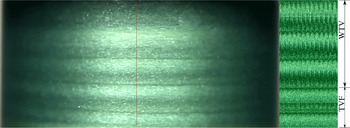
Co-existing state of ‘WTV
 $+$
TVF’ at
 $Re=115$
and
 $\unicode[STIX]{x1D719}=0.1$
during up-sweep runs. The space–time diagram (right) has been constructed by following the time evolution of a vertical line of one pixel width as marked on the left snapshot.

A closer comparison between the second and last panel on the top row of figure 8 confirms that the pattern in figure 9 (same as figure 7
b) is made up of two parts as (i) WTV on the top and (ii) TVF at the bottom, representing a ‘co-existing’ state, called ‘WTV
 $+$
TVF’, a part of which is a travelling wave and the remaining part is a stationary wave. This chimera-like new state appears as a primary bifurcation, see figure 5(a), only during ramp-up experiments when the particle volume fraction is
 $\unicode[STIX]{x1D719}\geqslant 0.05$
.
In the ramp-down experiments (figure 7
e–h and the bottom row of figure 8) at
 $\unicode[STIX]{x1D719}=0.1$
, the flow is initially in the WTV state (figure 7
h), and as
 $Re$
is decreased, it transitions into TVF (figure 7
g) at
 $Re\approx 152$
and subsequently to a new state of ‘spiral vortex flow’ (SVF), see figure 7(f), at
 $Re\approx 120.6$
. With further decrease in
 $Re$
, the flow returns back to the purely azimuthal CCF (figure 7
e) at
 $Re\leqslant 112$
. Referring to the pattern in figure 7(f) in which the Taylor vortices are aligned at some angle, the related space–time plot displayed in the second panel on the bottom row of figure 8 contains an array of inclined band, clearing indicating that this is a downward-propagating wave. In fact, the SVF can propagate up or down and represents a non-axisymmetric travelling wave which is absent in a Newtonian fluid when only inner cylinder rotates. Note that the SVF was found by Majji et al. (Reference Majji, Banerjee and Morris2018) in their experiments on suspension TCF.
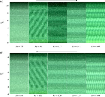
Space–time diagrams of patterns for up-sweep (top row) and down-sweep (bottom row) experiments at
 $\unicode[STIX]{x1D719}=0.2$
; each panel for specified
 $Re$
corresponds to a time window of approximately 2 seconds. The ramping rate is
 $\text{d}Re/\text{d}\unicode[STIX]{x1D70F}_{d}=0.0094$
.

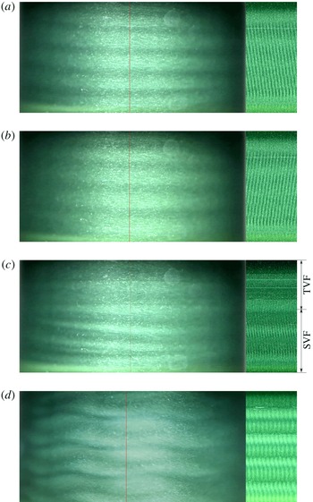
(a) Downward-propagating spiral vortex at
 $Re=91$
during up-sweep runs. (b) Upward-propagating spiral vortex at
 $Re=105$
during down-sweep runs. (c) Co-existing state of ‘TVF
 $+$
SVF’ at
 $Re=117$
during up-sweep runs. (d) WTV at
 $Re=166$
during up-sweep runs. For all cases,
 $\unicode[STIX]{x1D719}=0.2$
.

Figure 10 is an analogue of figure 8 (
 $\unicode[STIX]{x1D719}=0.1$
), displaying the space–time diagrams of up-sweep (top row) and down-sweep (bottom row) experiments for
 $\unicode[STIX]{x1D719}=0.2$
. In the ramp-up experiments, with increasing
 $Re$
the flow makes a transition from the featureless CCF (the left-most panels in top and bottom rows of figure 10) to spiral vortex flow at
 $Re\sim 85$
– a representative snapshot of the SVF (
 $Re=91$
) displayed in figure 11(a) is a downward-propagating spiral as confirmed from the backward inclined bands on the right panel of figure 11(a). As
 $Re$
is increased, the SVF transitions into a new combination state of ‘TVF
 $+$
SVF’ at
 $Re\sim 99$
, see the snapshot in figure 11(c). The latter is a combination of travelling and stationary waves which is confirmed from the space–time diagram on its right – in particular, the top two vortices represent stationary TVF, whereas the bottom three represent downward-propagating spiral vortices. This co-existing ‘TVF
 $+$
SVF’ state survives up to a Reynolds number of
 $Re\approx 136$
, beyond which it transitions to a stationary TVF state (the fourth panel on the top row of figure 10) and finally to a WTV state (figure 11
d) at
 $Re\geqslant 163$
. The space–time plots for the ramp-down protocol at
 $\unicode[STIX]{x1D719}=0.2$
(see panels on the bottom row in figure 10) confirms that the flow is initially in the WTV state; as the cylinder rotation speed is decreased, the flow transitions to TVF state, then to SVF and finally to the CCF state at
 $Re\leqslant 91$
. In particular, we find upward-propagating spiral vortices, see the snapshot in figure 11(b) and its space–time diagram (depicting ‘forward’ inclined bands) on its right.
Juxtaposing the observed patterns in figures 8 and 10 with two phase diagrams in figure 5, we find that there is a clear difference in the flow patterns seen during ramp-up and ramp-down protocols. The differences are found both in terms of new flow patterns seen over a range of Reynolds number as well as a change in the critical
 $Re$
for a pattern transition. While the non-axisymmetric spiral vortices were first reported by Majji et al. (Reference Majji, Banerjee and Morris2018) in suspension TCF, we have uncovered a new class of patterns (‘WTV
 $+$
TVF’ and ‘TVF
 $+$
SVF’), consisting of stationary and travelling waves living together along the axial direction of the cylinders, which have not been reported before in the context of TCF. Both represent an amalgamation of stationary Taylor vortices (TVF) in the one part of the TC cell with (i) an azimuthally propagating (WTV), or, (ii) an axially propagating (SVF) travelling wave in the remaining part. The internal structure and the stability of both co-existing patterns will be analysed in § 5 in terms of their radial–axial velocity fields.
Phase diagrams of patterns in
 $(Re,\unicode[STIX]{x1D6E4})$
plane in a TC cell of radius ratio
 $\unicode[STIX]{x1D702}=0.914$
. (a)
 $\unicode[STIX]{x1D719}=0.10$
(up-sweep) and (b)
 $\unicode[STIX]{x1D719}=0.20$
(up-sweep).

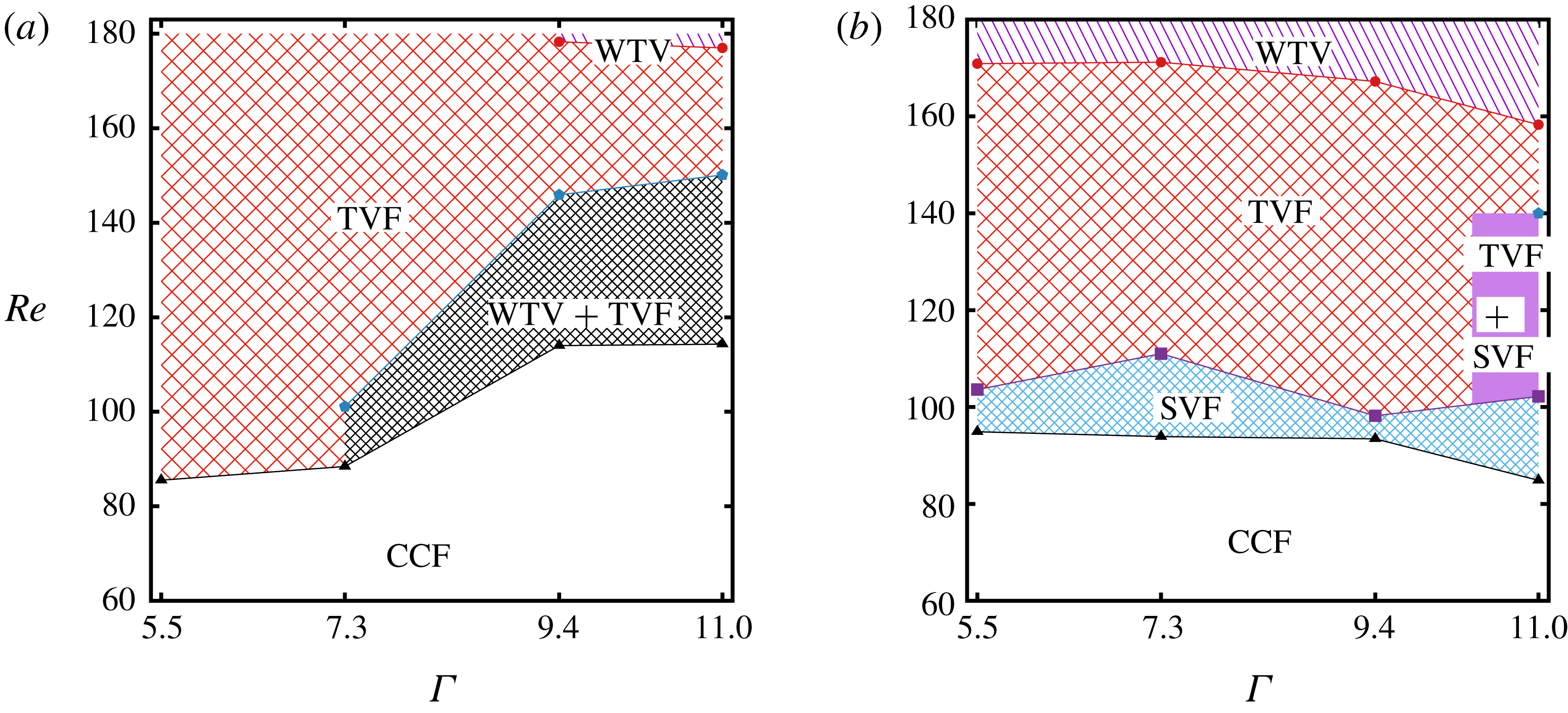
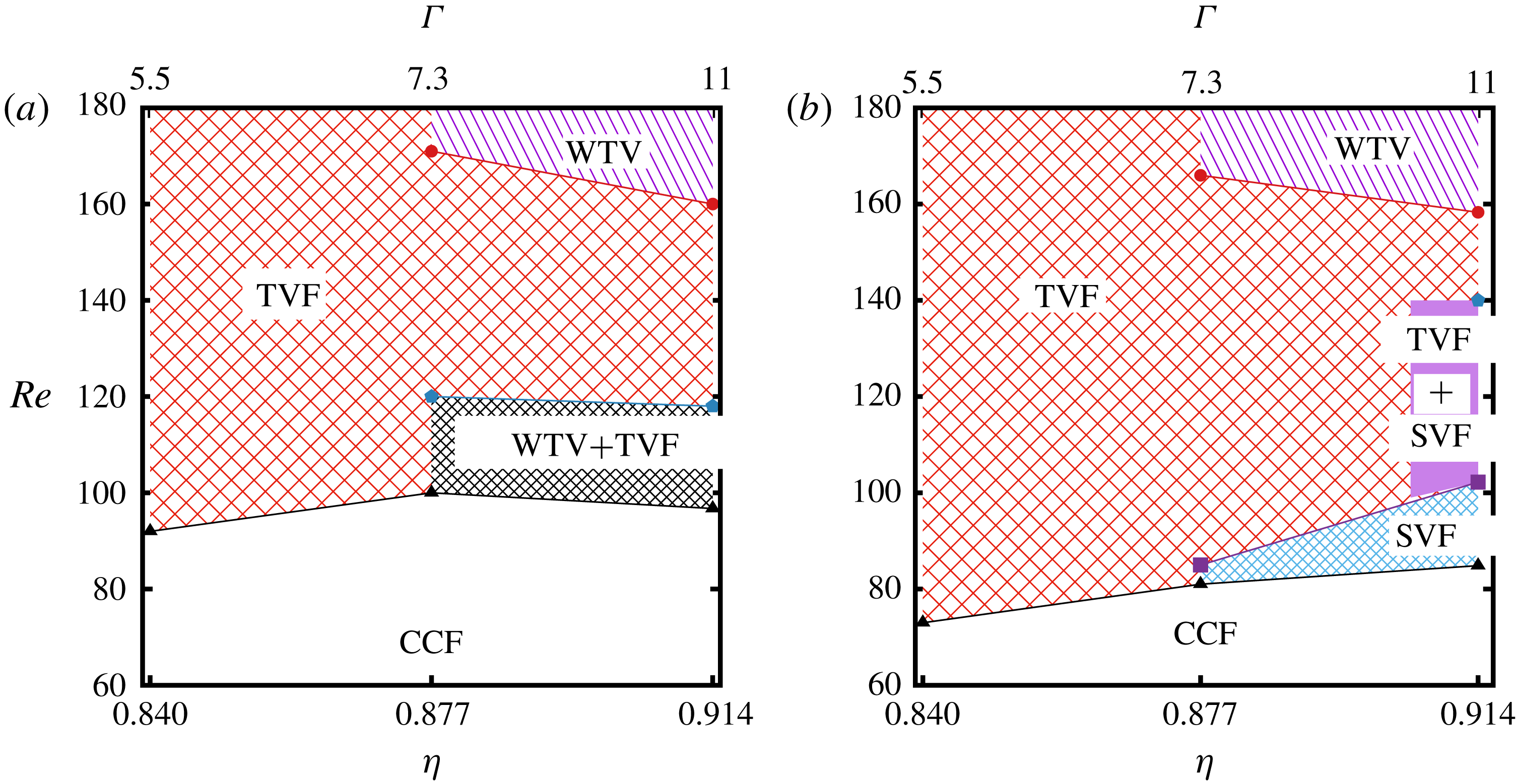
3.2.3 Effects of aspect ratio and radius ratio on phase diagram
All experiments described so far have been carried out in a Taylor–Couette cell of aspect ratio
 $\unicode[STIX]{x1D6E4}=h/\unicode[STIX]{x1D6FF}=11$
and the radius ratio
 $\unicode[STIX]{x1D702}=r_{i}/r_{o}=0.914$
with a rigid lid at the top of the TC cell. It is interesting to find out the possible effects of
 $\unicode[STIX]{x1D6E4}$
and
 $\unicode[STIX]{x1D702}$
on observed patterns – in particular, would the co-existing states survive for any
 $\unicode[STIX]{x1D6E4}$
and
 $\unicode[STIX]{x1D702}$
or are they a consequence of the small aspect ratio of our TC cell? To change
 $\unicode[STIX]{x1D6E4}$
, the height of the fluid level (
 $h$
) in the gap between two cylinders is changed by keeping the gap width (
 $\unicode[STIX]{x1D6FF}=1.5$
mm) constant and these experiments are performed for
 $\unicode[STIX]{x1D6E4}=5.5$
, 7.3, 9.4 and 11. On the other hand, to vary
 $\unicode[STIX]{x1D702}$
, outer cylinders with different radii (
 $r_{o}=17.5$
mm, 18.25 mm and 19 mm) are used to obtain
 $\unicode[STIX]{x1D702}=0.84$
, 0.877 and 0.914, by keeping the inner-cylinder radius (
 $r_{i}$
) and the fluid-level height (
 $h$
) fixed – in essence, both
 $\unicode[STIX]{x1D702}$
and
 $\unicode[STIX]{x1D6E4}$
are simultaneously varied in the latter experiments. Both sets of experiments have been carried out for
 $\unicode[STIX]{x1D719}=0.1$
and
 $\unicode[STIX]{x1D719}=0.2$
using up-sweep and down-sweep protocols with (i) a different outer cylinder (made of Plexiglas) and (ii) a ‘free surface’ at the top of the TC cell. For
 $\unicode[STIX]{x1D6E4}=11$
and
 $\unicode[STIX]{x1D702}=0.914$
, we have verified that the patterns depicted in figure 5 are recovered irrespective of the free surface, or, the rigid-lid boundary condition at the top.
Figures 12(a) and 12(b) display phase diagrams for
 $\unicode[STIX]{x1D719}=0.1$
and 0.2, respectively, in the (
 $Re,\unicode[STIX]{x1D6E4}$
)-plane for up-sweep experiments. Overall, the co-existing states like ‘WTV
 $+$
TVF’ and ‘TVF
 $+$
SVF’ are found only in the larger aspect-ratio TC cells; in particular, while the ‘WTV
 $+$
TVF’ state represents the primary bifurcation from the CCF state at
 $\unicode[STIX]{x1D6E4}\geqslant 7.3$
for
 $\unicode[STIX]{x1D719}=0.1$
, the ‘TVF
 $+$
SVF’ state is absent at
 $\unicode[STIX]{x1D6E4}\leqslant 9.4$
for
 $\unicode[STIX]{x1D719}=0.2$
. On the other hand, the non-axisymmetric states like the SVF survive even at
 $\unicode[STIX]{x1D6E4}=5.5$
for
 $\unicode[STIX]{x1D719}=0.2$
, see figure 12(b), and at
 $\unicode[STIX]{x1D6E4}\geqslant 7.4$
for
 $\unicode[STIX]{x1D719}=0.1$
(during down-sweep experiments, not shown). It is noteworthy that as the aspect ratio is decreased from
 $\unicode[STIX]{x1D6E4}=11$
, the onset of TVF occurs at a slightly lower value of
 $Re$
(figure 12
a), but the onset of WTV occurs at higher values of
 $Re$
(figure 12
b).
Phase diagrams of patterns in the
 $(Re,\unicode[STIX]{x1D702})$
plane where the fluid height
 $h$
is fixed but the radius of the outer cylinder
 $r_{o}$
is varied. (a)
 $\unicode[STIX]{x1D719}=0.10$
(up-sweep) and (b)
 $\unicode[STIX]{x1D719}=0.20$
(up-sweep).

The effects of changing
 $\unicode[STIX]{x1D702}$
and
 $\unicode[STIX]{x1D6E4}$
can be ascertained from figure 13. We find that both the non-axisymmetric patterns and the combination states are absent in wider (
 $\unicode[STIX]{x1D702}\leqslant 0.84$
) as well as in smaller aspect-ratio (
 $\unicode[STIX]{x1D6E4}\leqslant 5.5$
) TC cells. Collectively, figures 12 and 13 assert that all patterns observed in the present experiments (see the phase diagram in figure 5) are robust and devoid of (i) finite-size effects and (ii) the free surface or no-slip boundary condition at the top as long as the aspect ratio is
 $\unicode[STIX]{x1D6E4}\geqslant 7.3$
and the radius ratio is
 $\unicode[STIX]{x1D702}\geqslant 0.877$
.
Variations of critical Reynolds number for pattern transitions between different states, as obtained from consecutive ramp-up and ramp-down protocols, at
 $\unicode[STIX]{x1D719}=0.1$
(bottom rows) and 0.2 (top rows); see the text in § 3.2.4 for details on these experiments.

Hysteretic (sub-critical) nature of secondary transition from TVF
 $\rightarrow$
WTV with (a) varying
 $\unicode[STIX]{x1D719}$
at
 $\unicode[STIX]{x1D6E4}=11$
and (b) varying
 $\unicode[STIX]{x1D6E4}$
at
 $\unicode[STIX]{x1D719}=0.2$
.

3.2.4 Hysteresis and the secondary bifurcation TVF
 $\rightarrow$
WTV

To analyse hysteresis in pattern transitions, separate experiments have been carried out for particle volume fractions of
 $\unicode[STIX]{x1D719}=0.1$
and 0.2 as these two cases admit co-existing states of stationary and travelling waves during the onset of primary bifurcation from CCF. For each case (with a well-mixed suspension), starting from
 $Re\sim 75$
, the inner cylinder rotation is ramped-up quasi-steadily to
 $Re=180$
and the down-sweep is immediately initiated to return back to
 $Re=80$
at the same ramping rate – the related torque data, as measured in our rheometer, are discussed in the Appendix. Recall that all results described in the preceding sections §§ 3.2.1–3.2.3 correspond to up-sweep and down-sweep experiments in independent runs.
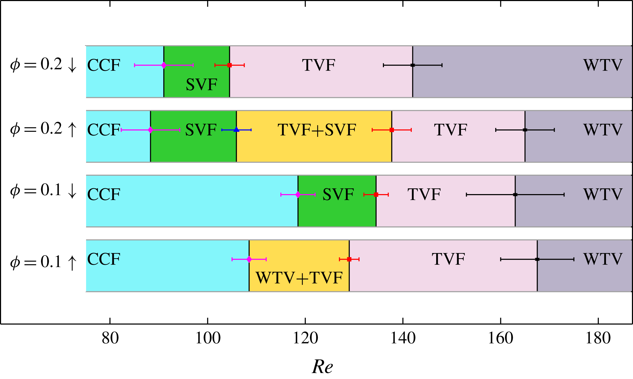
Figure 14 displays the ranges of Reynolds number over which each pattern persists in consecutive up-sweep and down-sweep experiments for
 $\unicode[STIX]{x1D719}=0.2$
(top rows) and 0.1 (bottom rows) – the error bars represent maximal variability in
 $Re$
, obtained from running images over three such experiments. It is seen that the primary bifurcation from CCF to a non-axisymmetric travelling wave (SVF) does not show hysteresis (i.e.
 $Re_{c}^{up}\approx Re_{c}^{down}$
) at
 $\unicode[STIX]{x1D719}=0.2$
, however, different patterns are uncovered during up-sweep and down-sweep at
 $\unicode[STIX]{x1D719}=0.1$
. In particular, the primary bifurcation at
 $\unicode[STIX]{x1D719}=0.1$
yields (i) a co-existing state of an axisymmetric stationary wave (TVF) and a non-axisymmetric azimuthally propagating wave (WTV) during up-sweep protocol and (ii) an axially propagating non-axisymmetric wave (SVF) during down-sweep protocol; decreasing the ramping rate from 0.015 to 0.005 did not affect the above pattern-transition scenario. These qualitative features of pattern transition remain similar to those depicted in figure 5(a,b) as obtained in independent up-sweep and down-sweep experiments.
At higher values of
 $Re>140$
, figure 14 indicates that the onset of secondary bifurcation from TVF to WTV is sub-critical in the sense that
 $Re_{c}^{up}>Re_{c}^{down}$
for both
 $\unicode[STIX]{x1D719}=0.1$
and 0.2, with the degree of sub-criticality (
 $Re_{c}^{up}-Re_{c}^{down}$
) increasing with increasing
 $\unicode[STIX]{x1D719}$
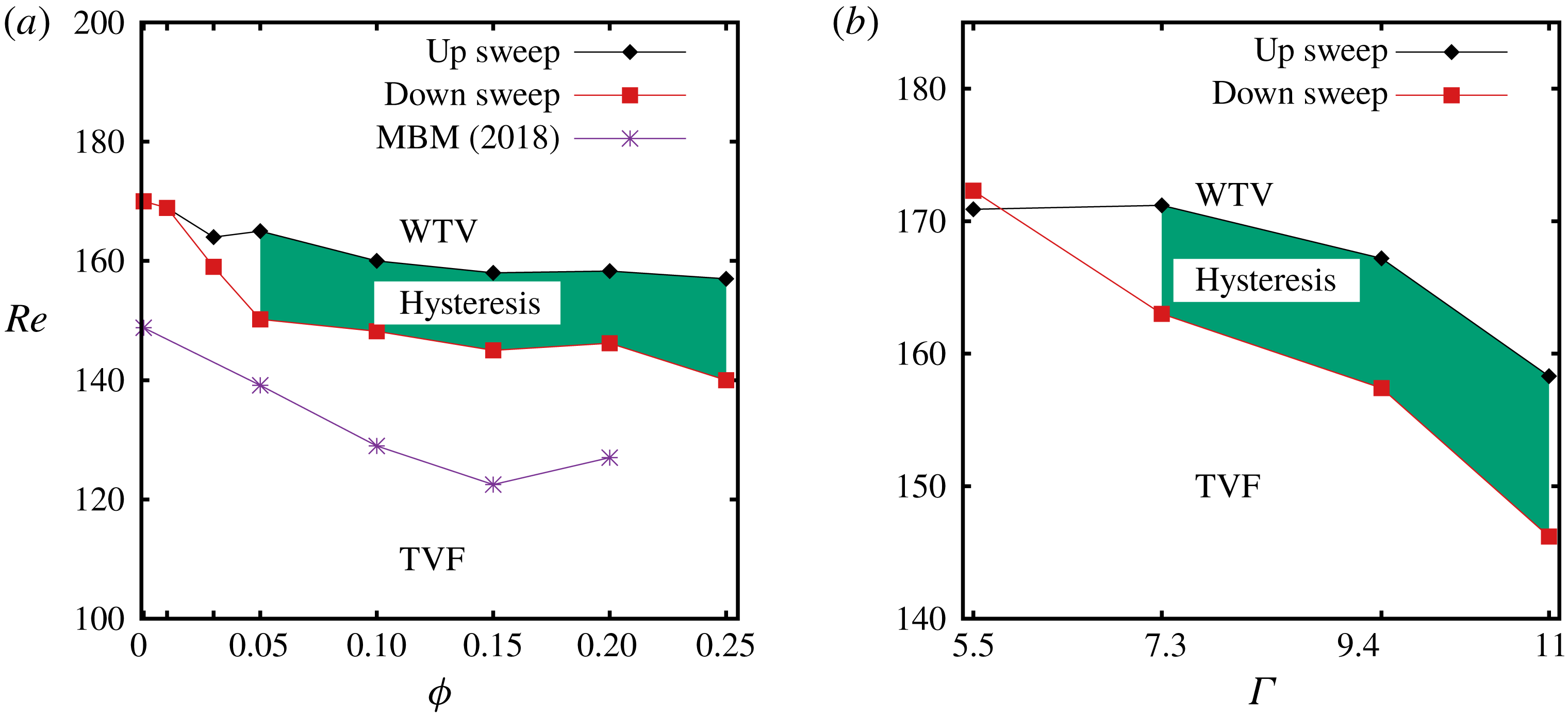
. The sub-critical nature of TVF
 $\rightarrow$
WTV transition holds for a range of
 $\unicode[STIX]{x1D719}>0$
, see figure 15(a), for a given aspect ratio
 $\unicode[STIX]{x1D6E4}=11$
– these data have been extracted from the phase diagram in figure 5. The effect of
 $\unicode[STIX]{x1D6E4}$
on TVF
 $\rightarrow$
WTV transition can be ascertained from figure 15(b) that corresponds to
 $\unicode[STIX]{x1D719}=0.2$
– the onset is expectedly delayed in smaller aspect-ratio cells, eventually inhibiting the formation of wavy Taylor vortices when the waviness of the Taylor vortices becomes comparable to
 $\unicode[STIX]{x1D6E4}$
. Collectively, figures 14 and 15 confirm that the secondary bifurcation, TVF
 $\leftrightarrow$
WTV, in suspension Taylor–Couette flow is sub-critical or hysteretic, in contrast to its super-critical nature in the TCF of a Newtonian fluid.
3.2.5 Wave speed in WTV and SVF
Power spectra of scattered light intensity in the WTV regime for (a) Newtonian fluid (
 $\unicode[STIX]{x1D719}=0$
) and (b) suspension (
 $\unicode[STIX]{x1D719}=0.1$
). (c) Variations of normalized wave speed with
 $\unicode[STIX]{x1D719}$
for WTV (at
 $Re=182$
) and SVF; triangles and squares (with error bars) represent wave speeds of SVF as calculated from ‘light-intensity spectra’ and the ‘Hough transform’, respectively. (d) Histogram of the slope data for SVF, obtained from the Hough transform (see the text in § 3.2.5 for details), at
 $\unicode[STIX]{x1D719}=5\,\%$
and
 $Re=121$
.

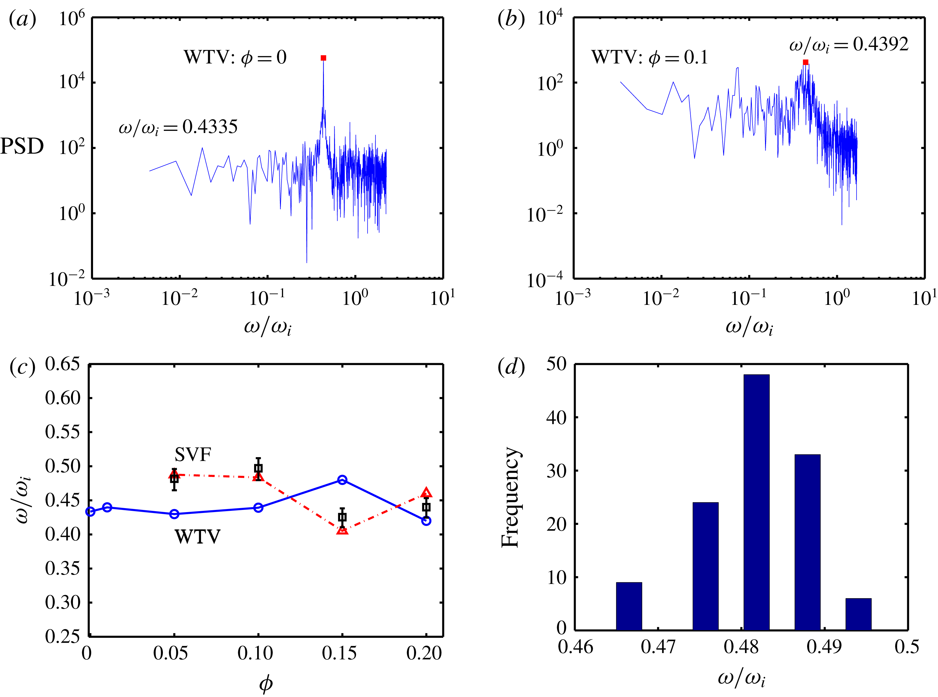
While the wavy Taylor vortices, such in figure 7(d,h), are azimuthally propagating waves, the spiral vortices, such as in figure 11(a,b), represent axially propagating (upward or downward travelling) waves. We have measured the speed of wavy Taylor vortices from the scattered light-intensity spectra as described in King et al. (Reference King, Li, Lee, Swinney and Marcus1984). In particular, the change in the intensity of the wave for
 $1/4$
th axial wavelength is used to construct a time series whose fast Fourier transform yields the underlying power spectra. Figures 16(a) and 16(b) display two such power spectra for WTV at
 $Re=182$
with
 $\unicode[STIX]{x1D719}=0$
(pure fluid) and
 $\unicode[STIX]{x1D719}=0.1$
, respectively – the peak in each panel represents the frequency of the wave. The peak frequency, normalized with the rotational speed of the inner cylinder, is plotted versus particle volume fraction in figure 16(c), denoted by circles.
The same procedure is followed to estimate the speed of the spiral vortices which can be positive or negative depending on whether it is propagating up or down axially. Recall that the slope of the inclined bands in the space–time diagrams of SVF (such as in the second panels of figure 10) is a measure of the speed of the spiral vortices – this has been extracted using a Hough transform which involves a sequence of operations: (i) identify the lines of constant phase in the space–time plots of SVF, (ii) measure the slope of these lines and (iii) generate the histogram of such slope data. A typical histogram of the slope data for SVF is shown in figure 16(d) for the case of
 $\unicode[STIX]{x1D719}=0.1$
and
 $Re=110$
– the mean of this histogram is the average speed with which the spiral vortices propagate axially up or down. The latter data are denoted by square symbols (with error bars representing the variance of the histogram, such as in panel
 $d$
) in figure 16(c) that agree well with wave-speed measurements of SVF from light-intensity spectra (denoted by triangles).
It is clear from figure 16(c) that, for both wavy Taylor and spiral vortices, the normalized wave speed is approximately one half of the rotational speed of the cylinder, and neither seem to depend on the particle volume fraction for
 $\unicode[STIX]{x1D719}\leqslant 0.2$
. Note that Majji et al. (Reference Majji, Banerjee and Morris2018) measured the wave speed of SVF from image analysis (their figure 18), and our data agree with their finding.
4 Velocity measurements and the characteristics of Taylor vortices
Recall from § 2.4 that we have used a refractive-index-matched solvent such that the ‘suspension’ particles are invisible, and the fluid velocity field is obtained from the analyses of PIV (particle image velocimetry) image pairs which contain information about the scattered light of ‘seeded’ fluorescent particles. Since the particle Reynolds number and Stokes number are
 $O(10^{-4})$
or less (see table 1), the particles are expected to follow fluid velocity field. We have not made any effort to separately measure the velocity of the particle phase or its concentration profile.
The velocity measurements are carried out for particle volume fractions of
 $\unicode[STIX]{x1D719}=0$
, 0.03, 0.05, 0.1 and 0.15 for a range of Reynolds numbers
 $25\leqslant Re\leqslant 182$
in a Taylor–Couette cell of aspect ratio
 $\unicode[STIX]{x1D6E4}=11$
and radius ratio
 $\unicode[STIX]{x1D702}=0.914$
with a free surface on the top. Note that these measurements are restricted to
 $\unicode[STIX]{x1D719}\leqslant 0.15$
since the PIV images of suspensions at higher particle loadings are found to be of poor quality due to the difficulties in obtaining precise refractive-index matching at
 $\unicode[STIX]{x1D719}>0.15$
. For stationary patterns such as CCF and TVF, the instantaneous PIV velocity is time averaged over the above time window to yield information on the average velocity field (
 $v_{\unicode[STIX]{x1D703}},v_{r},v_{z}$
) as discussed in §§ 4.1 and 4.2. On the other hand, for non-stationary patterns (such as WTV and SVF), the instantaneous velocity data in the (
 $r,z$
)-plane will be presented in § 5 in order to characterize the internal structure of the presently uncovered co-existing states like ‘TVF
 $+$
SVF’ and ‘TVF
 $+$
WTV’.
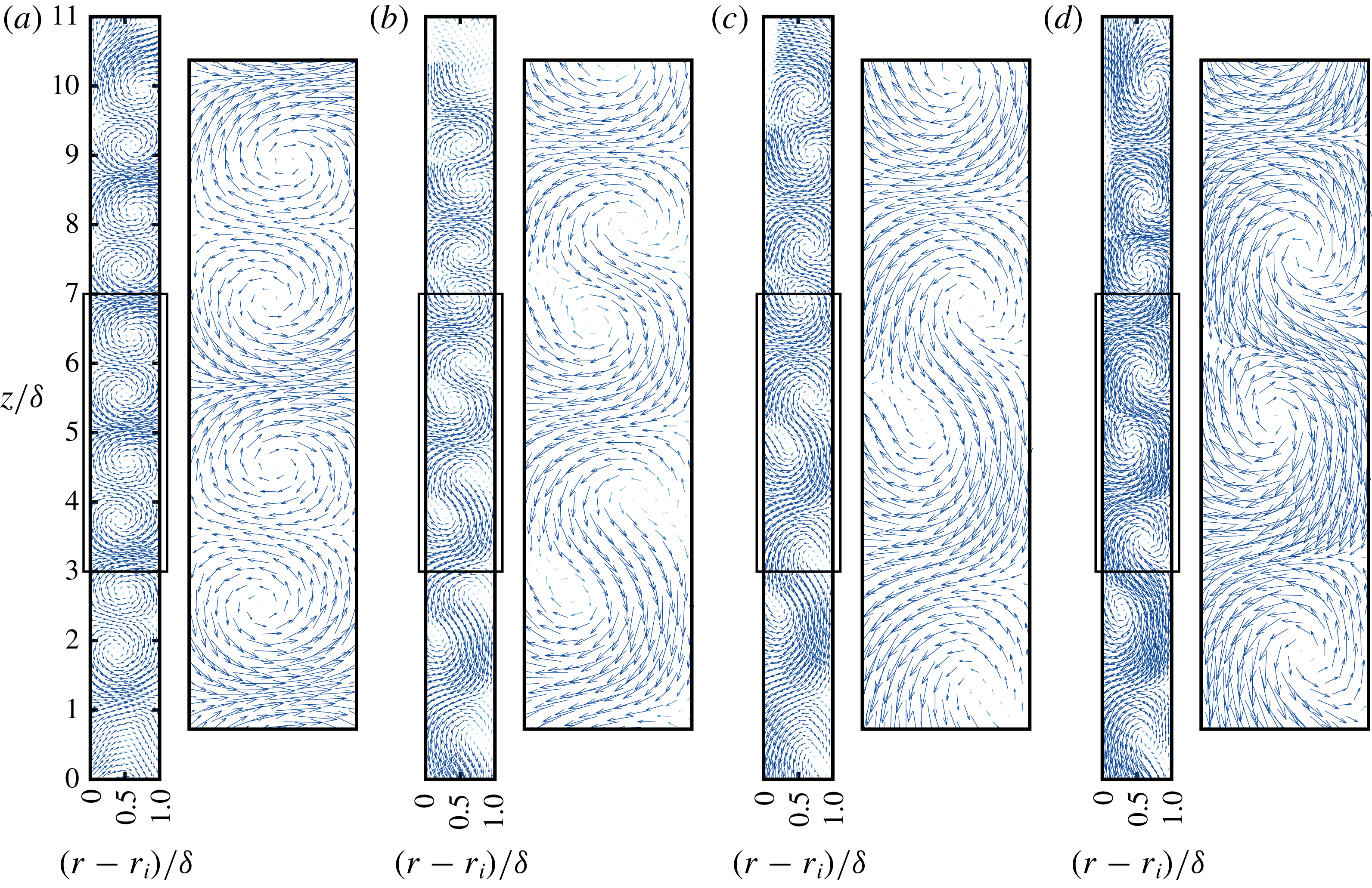
Average velocity vectors in the (
 $r,z$
) plane for stationary Taylor vortices (TVF at
 $Re=143$
) with (a)
 $\unicode[STIX]{x1D719}=0$
, (b)
 $\unicode[STIX]{x1D719}=0.05$
, (c)
 $\unicode[STIX]{x1D719}=0.10$
and (d)
 $\unicode[STIX]{x1D719}=0.15$
. In each panel, the right image is a zoomed version of the marked box on the left image of the full (
 $r,z$
) plane; for clarity, every fifth vector is shown in each image.

In this section, we restrict ourselves to stationary Taylor vortices that are characterized by non-zero radial and axial velocities (
 $v_{r}\neq 0$
and
 $v_{z}\neq 0$
). The measured (
 $v_{r},v_{z}$
) velocity field helped to answer four specific questions. (i) How does the fluctuation energy depend on particle loading in the TVF regime? (ii) Are the Taylor vortices in suspension TCF symmetric as in Newtonian TCF? (iii) Do they represent perfectly harmonic waves? (iv) Does the radial transport induced by Taylor vortices depend on particle loading?
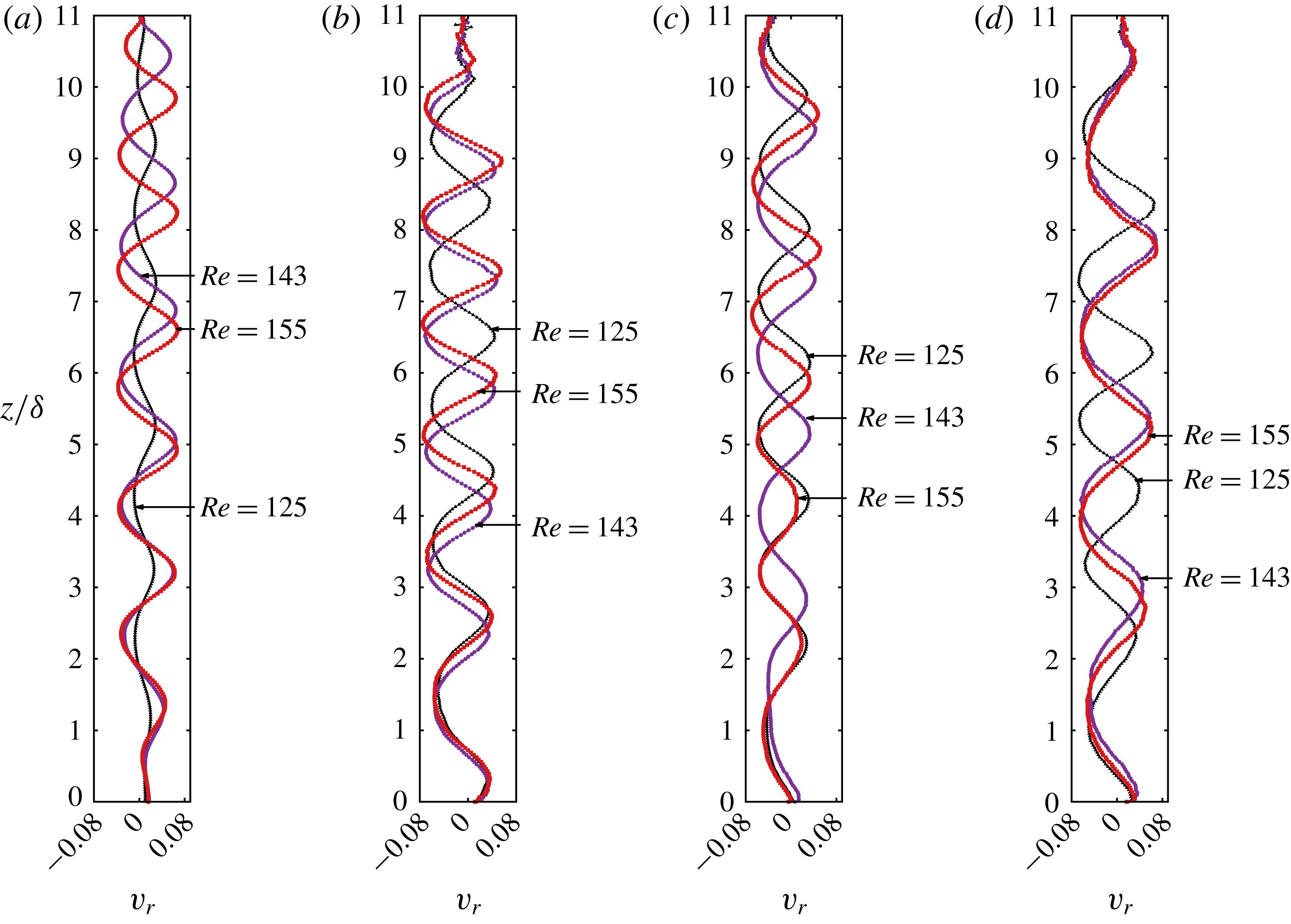
Axial variations of the dimensionless radial velocity,
 $v_{r}/r_{i}\unicode[STIX]{x1D714}_{i}$
, at the mid-gap
 $r=r_{i}+\unicode[STIX]{x1D6FF}/2$
for different
 $Re$
. (a) Newtonian
 $\unicode[STIX]{x1D719}=0$
, (b)
 $\unicode[STIX]{x1D719}=0.05$
, (c)
 $\unicode[STIX]{x1D719}=0.10$
and (d)
 $\unicode[STIX]{x1D719}=0.15$
.

4.1 Axial–radial velocities and kinetic energy
Figure 17 displays the velocity vectors in the (
 $r,z$
) plane for various particle volume fractions – for all cases, the Reynolds number is
 $Re=143$
that belongs to the TVF regime for all
 $\unicode[STIX]{x1D719}$
. For the Newtonian case in figure 17(a), the well-defined pairs of nearly symmetric Taylor vortices are established along the length of the cylinder – a zoomed in version of the velocity field around the mid-height of the TC cell, containing two pairs of Taylor vortices, is displayed next to the full image. On the other hand, for suspension TCF in figure 17(b–d), we find that the Taylor vortices appear to be elongated and the vortex centres are slightly offset from the mid-gap location
 $r=r_{i}+\unicode[STIX]{x1D6FF}/2$
.
Figure 18 displays the axial profiles of dimensionless radial velocity,
 $v_{r}/(r_{i}\unicode[STIX]{x1D714}_{i})$
, evaluated at the mid-gap
 $r=r_{i}+\unicode[STIX]{x1D6FF}/2$
, for different Reynolds numbers: (a), (b), (c) and (d) refer to
 $\unicode[STIX]{x1D719}=0$
,
 $\unicode[STIX]{x1D719}=0.05$
,
 $\unicode[STIX]{x1D719}=0.10$
and
 $\unicode[STIX]{x1D719}=0.15$
, respectively. Note that the zero crossings of the radial velocity profile are identified as approximate locations of the centres of Taylor vortices in Newtonian TCF. It is seen that the radial velocities of the top and bottom vortex pairs are markedly influenced by the end effects of the TC cell, irrespective of the value of
 $\unicode[STIX]{x1D719}$
– recall that there is a free surface at the top and a rigid lid at the bottom of our TC cell. Within the bulk of the TC cell,
 $2\leqslant z/\unicode[STIX]{x1D6FF}\leqslant 9$
, the mid-gap radial velocity is approximately symmetric (
 $v_{r}^{max}\approx v_{r}^{min}$
) in a Newtonian fluid (a), however, (b–d) indicate asymmetric nature of the radial velocity in a suspension – this is an important difference which will be quantified in § 4.2.
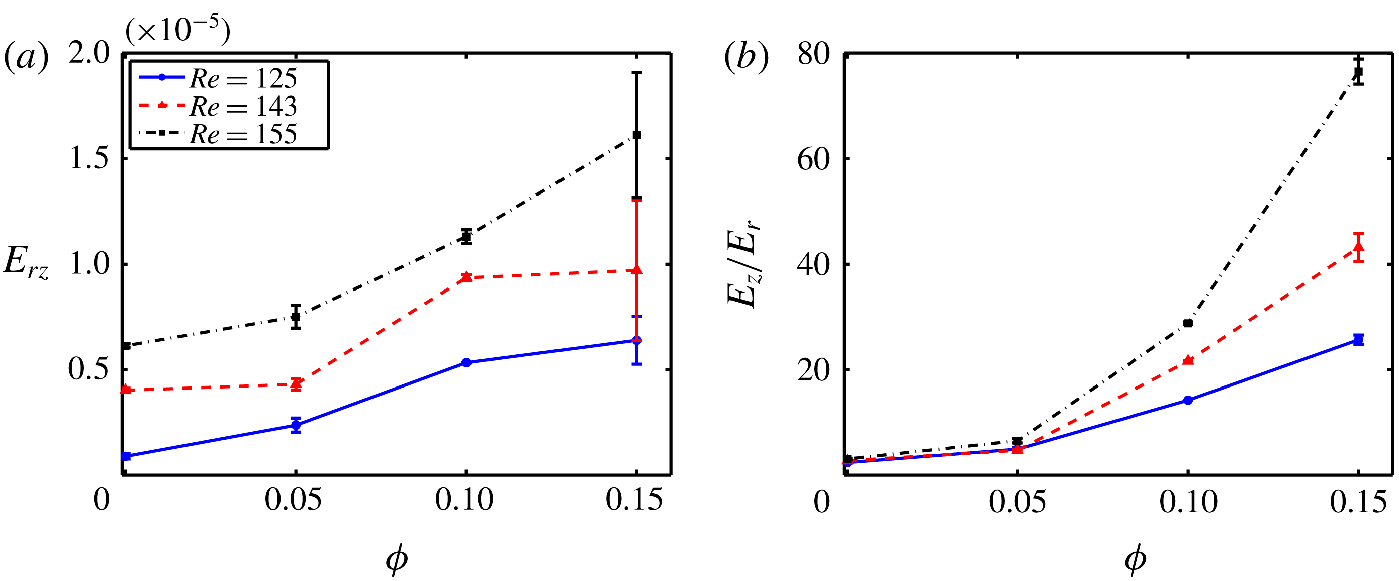
(a) Variations of dimensionless axial–radial kinetic energy,
 $E_{rz}=(E_{r}+E_{z})/\unicode[STIX]{x1D714}_{i}^{2}r_{i}^{2}$
, with particle volume fraction at different Reynolds numbers. (b) Ratio of axial-to-radial energy,
 $E_{z}/E_{r}$
, versus
 $\unicode[STIX]{x1D719}$
.

The data from figure 17 are used to estimate the specific kinetic energy associated with radial and axial motions,
 $$\begin{eqnarray}\displaystyle & \displaystyle E_{r}=\frac{1}{2}\langle u_{r}^{2}\rangle _{rz}=\frac{1}{2}\mathop{\sum }_{z=0}^{z=h}\mathop{\sum }_{r=r_{i}}^{r=r_{o}}u_{r}^{2} & \displaystyle\end{eqnarray}$$
 $$\begin{eqnarray}\displaystyle & \displaystyle E_{z}=\frac{1}{2}\langle u_{z}^{2}\rangle _{rz}=\frac{1}{2}\mathop{\sum }_{z=0}^{z=h}\mathop{\sum }_{r=r_{i}}^{r=r_{o}}u_{z}^{2} & \displaystyle\end{eqnarray}$$
respectively. Figure 19(a) shows the variations of the normalized axial–radial kinetic energy,
 $E_{rz}=(E_{r}+E_{z})/\unicode[STIX]{x1D714}_{i}^{2}r_{i}^{2}$
, with particle volume fraction at different values of
 $Re$
, evaluated over the whole domain of
 $z/\unicode[STIX]{x1D6FF}\in (0,11)$
. It is seen that
 $E_{rz}$
increases with increasing particle loading (
 $\unicode[STIX]{x1D719}$
) at any
 $Re$
which is expected since the shear viscosity increases in the same limit. This implies that, to maintain a given
 $Re$
, the inner-cylinder rotational speed should be increased with increasing particle volume fraction. The dependence of the axial–radial energy ratio
 $E_{z}/E_{r}$
on
 $\unicode[STIX]{x1D719}$
is shown in figure 19(b). It is seen that the axial kinetic energy is much larger than its radial component for all three values of
 $Re$
, and it increases with increasing
 $\unicode[STIX]{x1D719}$
. We may conclude from figure 19 that the enhanced velocity fluctuations in the TVF regime of suspension TCF are triggered by the particles.
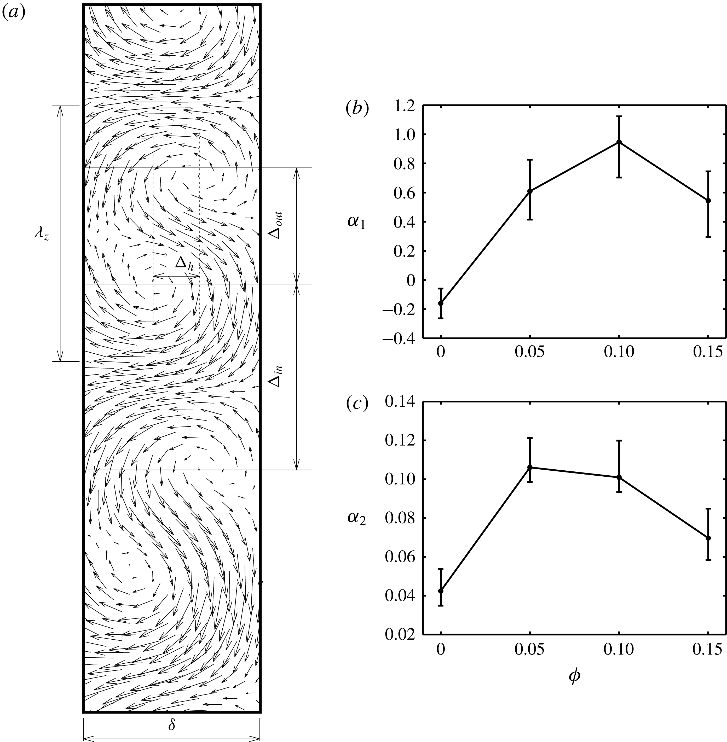
(a) Definition of different length scales for vortex flows in the
 $(r,z)$
-plane. Variations with particle volume fraction of (b) the degree of vertical anharmonicity
 $\unicode[STIX]{x1D6FC}_{1}$
as defined in (4.3) and (c) the degree of horizontal anharmonicity
 $\unicode[STIX]{x1D6FC}_{2}$
as defined in (4.4). All patterns represent stationary Taylor vortices (TVF) at
 $Re=143$
.

4.2 Suspension Taylor vortices: anharmonicity, asymmetry and radial transport
We have noted in figure 17(b–d) that the (
 $r,z$
) velocity field of stationary Taylor vortices in a suspension looks different from that of its Newtonian counterpart in figure 17(a) on two counts: (i) the distance between two successive vortex centres is seen to vary with particle loading
 $\unicode[STIX]{x1D719}$
and (ii) the vortex centres are not aligned for
 $\unicode[STIX]{x1D719}\neq 0$
. These structural features can be quantified in terms of three geometric parameters as marked in the sketch in figure 20(a): (i)
 $\unicode[STIX]{x1D6E5}_{in}$
and
 $\unicode[STIX]{x1D6E5}_{out}$
denote the axial distances between two successive vortex centres with (radially) inward and outward flows, respectively, with reference to the rotating inner cylinder, and (ii)
 $\unicode[STIX]{x1D6E5}_{h}$
is the mean radial offset between two successive counter-rotating vortex centres. For
 $\unicode[STIX]{x1D6E5}_{in}=\unicode[STIX]{x1D6E5}_{out}$
and
 $\unicode[STIX]{x1D6E5}_{h}=0$
, the axial array of counter-rotating Taylor vortices can be represented by harmonic waves, which holds perfectly near the onset Reynolds number
 $Re\sim Re_{c}$
. The anharmonicity of Taylor vortices can therefore be defined in terms of two dimensionless geometric parameters: (i) the degree of ‘vertical’ anharmonicity of the vortex flow is
 $$\begin{eqnarray}\displaystyle \unicode[STIX]{x1D6FC}_{1}=\frac{\unicode[STIX]{x1D6E5}_{in}}{\unicode[STIX]{x1D6E5}_{out}}-1, & & \displaystyle\end{eqnarray}$$
and (ii) the degree of ‘horizontal’ anharmonicity
 $$\begin{eqnarray}\displaystyle \unicode[STIX]{x1D6FC}_{2}=\frac{\unicode[STIX]{x1D6E5}_{h}}{\unicode[STIX]{x1D6FF}}, & & \displaystyle\end{eqnarray}$$
where
 $\unicode[STIX]{x1D6FF}$
the is the Couette gap. For the Reynolds number of
 $Re=143$
, the variations of
 $\unicode[STIX]{x1D6FC}_{1}$
and
 $\unicode[STIX]{x1D6FC}_{2}$
are shown in figures 20(b) and 20(c), respectively. In general we find that
 $\unicode[STIX]{x1D6FC}_{i}(\unicode[STIX]{x1D719}\neq 0)>\unicode[STIX]{x1D6FC}_{i}(\unicode[STIX]{x1D719})$
, indicating increased anharmonicity of Taylor vortices in a suspension.
The radial velocity profiles in figure 18 can be characterized in terms of the following quantity (Hoffmann et al. Reference Hoffmann, Lücke and Pinter2004),
 $$\begin{eqnarray}\displaystyle {\mathcal{P}}(r=r_{i}+\unicode[STIX]{x1D6FF}/2)=\frac{\displaystyle \int _{-\unicode[STIX]{x1D706}_{z}/2}^{\unicode[STIX]{x1D706}_{z}/2}|v_{r}(z,r)-v_{r}(-z,r)|\,\text{d}z}{\displaystyle \int _{-\unicode[STIX]{x1D706}_{z}/2}^{\unicode[STIX]{x1D706}_{z}/2}|v_{r}(z,r)+v_{r}(-z,r)|\,\text{d}z}, & & \displaystyle\end{eqnarray}$$
at the mid-gap (
 $r=r_{i}+\unicode[STIX]{x1D6FF}/2$
), where
 $\unicode[STIX]{x1D706}_{z}=2\unicode[STIX]{x03C0}/k$
is the axial wavelength of the vortices. This (4.5) is called the ‘asymmetry’ parameter (Hoffmann et al.
Reference Hoffmann, Lücke and Pinter2004; Abcha et al.
Reference Abcha, Crumeyrolle, Ezersky and Mutabazi2013) which has been used in the literature to distinguish between TVF and SVF since it is known that
 ${\mathcal{P}}\approx 0$
for Taylor vortices, but
 ${\mathcal{P}}=O(1)$
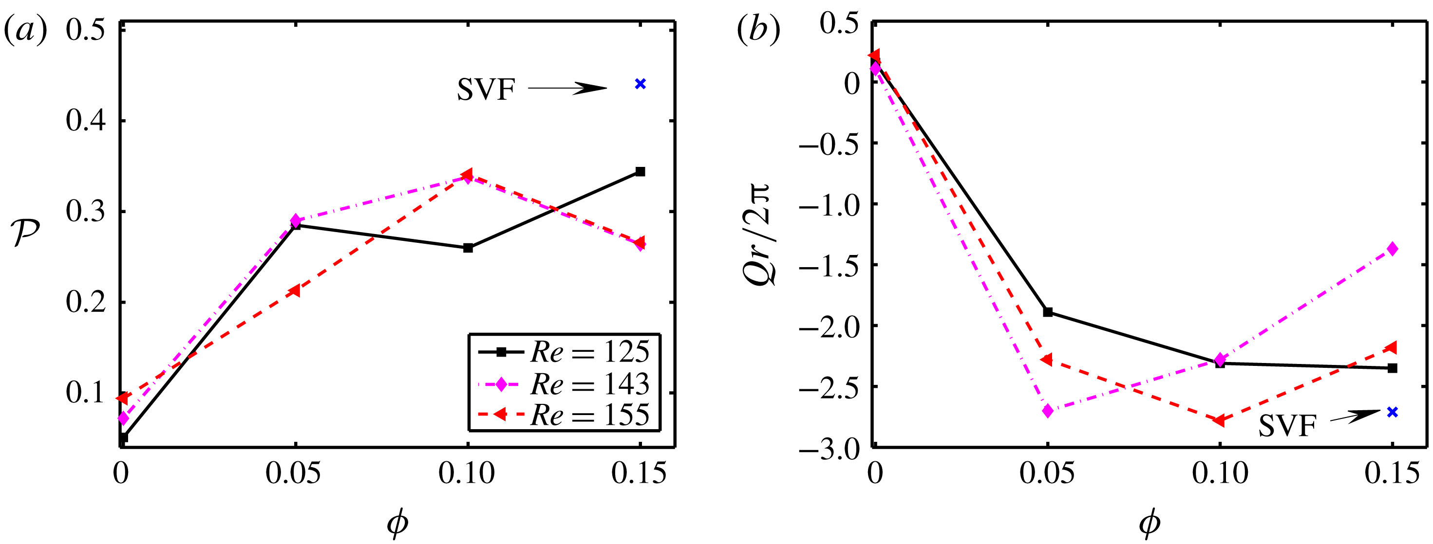
for spiral vortices in incompressible Taylor–Couette flows. Figure 21(a) shows the variations of
 ${\mathcal{P}}$
with
 $\unicode[STIX]{x1D719}$
for different
 $Re$
. It is clear that suspension Taylor vortices are more asymmetric than their Newtonian counterparts. The solitary data point (a cross) at
 $\unicode[STIX]{x1D719}=0.15$
in figure 21(a) corresponds to spiral vortex flow (SVF at
 $Re=100$
, see figure 5) for which
 ${\mathcal{P}}\approx 0.44$
, reconfirming previous observations (Abcha et al.
Reference Abcha, Crumeyrolle, Ezersky and Mutabazi2013) of increased asymmetry of SVF compared to that of TVF (in a Newtonian fluid).
(a) Effects of Reynolds number on the asymmetry parameter
 ${\mathcal{P}}$
(4.5) at different particle volume fractions. (b) Variations of dimensionless radial flow rate (
 $Q_{r}$
), equation (4.6), with particle volume fraction at different Reynolds numbers. The solitary data (cross) in both panels represents SVF at
 $Re=110$
.

Using the radial velocity profiles such as in figure 18, the local radial flow rate at the mid-gap,
 $r=r_{i}+\unicode[STIX]{x1D6FF}/2$
, integrated over one axial wavelength (
 $\unicode[STIX]{x1D706}_{z}$
) of Taylor vortices, can be calculated from
 $$\begin{eqnarray}\displaystyle Q_{r}=2\unicode[STIX]{x03C0}r\int _{-\unicode[STIX]{x1D706}_{z}/2}^{\unicode[STIX]{x1D706}_{z}/2}v_{r}(r,z)\,\text{d}z=2\unicode[STIX]{x03C0}(1+\unicode[STIX]{x1D709}/2)\int _{-\unicode[STIX]{x1D706}_{z}/2\unicode[STIX]{x1D6FF}}^{\unicode[STIX]{x1D706}_{z}/2\unicode[STIX]{x1D6FF}}v_{r}(r=1+\unicode[STIX]{x1D709}/2,z)\,\text{d}z, & & \displaystyle\end{eqnarray}$$
where
 $\unicode[STIX]{x1D709}=(1-\unicode[STIX]{x1D702})/\unicode[STIX]{x1D702}$
, with the factor
 $2\unicode[STIX]{x03C0}$
coming from the ansatz of flow homogeneity along the azimuthal direction (
 $\unicode[STIX]{x1D703}$
); note that the second equality in (4.6) represents the dimensionless flow rate. The variations of
 $Q_{r}$
with
 $\unicode[STIX]{x1D719}$
are shown in figure 21(b) for different
 $Re$
. It is seen that the radial flow rate in Taylor vortices is significantly enhanced in a suspension (
 $\unicode[STIX]{x1D719}\neq 0$
) in comparison to its Newtonian counterpart (
 $\unicode[STIX]{x1D719}=0$
). In addition, the solitary data for the spiral vortices (SVF) (marked by a cross in figure 21
b) at
 $Re=100$
confirms that the suspension Taylor vortices are comparable to their spiral counterparts in terms of radial transport.
Recall from figures 20 and 21 that the
 $\unicode[STIX]{x1D719}$
-dependences of both
 $\unicode[STIX]{x1D6FC}_{1}$
(figure 20
b) and
 $\unicode[STIX]{x1D6FC}_{2}$
(figure 20
c) as well as those of
 ${\mathcal{P}}$
(figure 21
a) and
 $Q_{r}$
(figure 21
b) are non-monotonic at higher Reynolds number (
 $Re\geqslant 143$
). Collectively, this implies that the asymmetry, anharmonicity and radial transport of Taylor vortices are most enhanced at some intermediate value of the particle volume fraction (
 $\unicode[STIX]{x1D719}\sim 0.1$
) beyond which the suspension Taylor vortices possibly undergo structural transitions to become more symmetric and harmonic. Velocity data at higher particle loadings (
 $\unicode[STIX]{x1D719}\geqslant 0.2$
) would be needed to make any concrete conclusion on the latter issue.
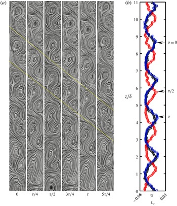
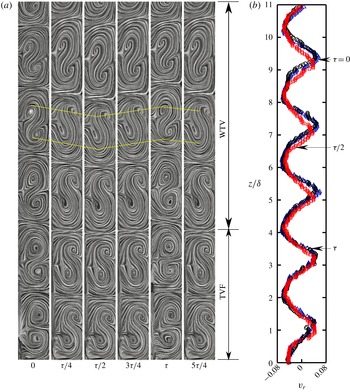
(a) Instantaneous streamlines of SVF (
 $Re=100$
and
 $\unicode[STIX]{x1D719}=0.15$
), and (b) its mid-gap radial velocity profile. Panel (a) contains six successive images of streamline patterns at times
 $t\approx n_{1}\unicode[STIX]{x1D70F}$
,
 $n_{2}\unicode[STIX]{x1D70F}+\unicode[STIX]{x1D70F}/4$
,
 $n_{3}\unicode[STIX]{x1D70F}+\unicode[STIX]{x1D70F}/2$
,
 $n_{4}\unicode[STIX]{x1D70F}+3\unicode[STIX]{x1D70F}/4$
,
 $n_{5}\unicode[STIX]{x1D70F}+\unicode[STIX]{x1D70F}$
and
 $n_{6}\unicode[STIX]{x1D70F}+5\unicode[STIX]{x1D70F}/4$
, where
 $\unicode[STIX]{x1D70F}\approx 0.281$
s is the time period of SVF (figure 16
c,
 $\unicode[STIX]{x1D70F}\equiv \unicode[STIX]{x1D70F}_{SVF}\approx 4\unicode[STIX]{x03C0}/\unicode[STIX]{x1D714}_{i}$
, with
 $\unicode[STIX]{x1D714}_{i}$
being the rotational speed of inner cylinder) and
 $n_{i}\gg 1$
is an integer.

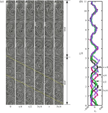
Same as figure 22, but for the co-existing state of ‘TVF
 $+$
SVF’ at
 $Re=120$
and
 $\unicode[STIX]{x1D719}=0.15$
. Here,
 $\unicode[STIX]{x1D70F}\equiv \unicode[STIX]{x1D70F}_{SVF}\approx 0.234$
.

Same as figure 23(a,b), but for the co-existing state of ‘WTV
 $+$
TVF’ at
 $Re=110$
and
 $\unicode[STIX]{x1D719}=0.1$
. Here,
 $\unicode[STIX]{x1D70F}\equiv \unicode[STIX]{x1D70F}_{WTV}\approx 0.328$
.

5 Skeletons and stability of co-existing stationary and travelling vortices
Since the wavy Taylor vortices and spiral vortices represent travelling waves, the averaging of PIV velocity data, procured over a time window, is complicated, and hence we have restricted ourselves to presenting the instantaneous velocity field as obtained from two successive PIV images, separated by a time delay of
 $\unicode[STIX]{x0394}t_{rz}\in (200,500)~\unicode[STIX]{x03BC}\text{s}$
. Such velocity data are used to generate instantaneous patterns of streamlines, see figure 22(a) for the temporal evolution of the internal structures of spiral vortices in the radial–axial plane; the parameter values are
 $\unicode[STIX]{x1D719}=0.15$
and
 $Re=110$
. The counter-rotating vortex pairs and their centres are clearly identified in each image – the asymmetry in the arrangement of the vortex centres is also evident. This represents a downward-propagating spiral vortex flow (SVF) which can be ascertained from the movement of the vortex pair bounded by two yellow lines. Note that the streamline plots have been drawn using the ‘surface-LIC’ (surface line-integral convolution) module of the Paraview software (Ahrens et al.
Reference Ahrens, Geveci, Law, Hansen and Johnson2005) – this helps in visualization by indicating an apparent motion along the direction of the vector field which is evident in figure 22(a).
Since the time period of the SVF state in figure 22(a) is
 $\unicode[STIX]{x1D70F}_{SVF}\approx 2\unicode[STIX]{x1D70F}_{i}=4\unicode[STIX]{x03C0}/\unicode[STIX]{x1D714}_{i}\approx 0.281~\text{s}$
(see figure 16
c) and the camera has a frame rate of 4.454 fps (i.e. the successive image pairs procured by the PIV camera are separated by a time delay of
 $\unicode[STIX]{x1D70F}_{cam}=1/4.454\approx 0.2245$
s), the streamline plots in figure 22(a) represent a sequence of images of the SVF, separated by a ‘longer’ time interval of
 $[(n_{i+1}-n_{i})+1/4]\unicode[STIX]{x1D70F}_{SVF}$
, where
 $n_{i}$
is a large integer. More specifically, for each PIV run, 500 image pairs are procured by the camera over a time span of approximately
 $400\unicode[STIX]{x1D70F}_{SVF}$
, with each pair yielding a streamline plot; five such streamline plots are selected from them, with two successive ones being approximately separated by
 $(\unicode[STIX]{x0394}n_{i}\unicode[STIX]{x1D70F}_{SVF}+\unicode[STIX]{x1D70F}_{SVF}/4)$
with
 $\unicode[STIX]{x0394}n_{i}\gg 1$
, to generate figure 22(a). It is clear from figure 22(a) that both the radial–axial plane structure of the vortex arrays and the spatio-temporal periodicity of SVF are maintained even after a long time, suggesting that the SVF is a stable state. The instantaneous radial velocity field has been extracted from the velocity data of figure 22(a); the axial profiles of the radial velocity,
 $v_{r}/\unicode[STIX]{x1D714}_{i}r_{i}$
, evaluated at the mid-gap
 $r=r_{i}+\unicode[STIX]{x1D6FF}/2$
are shown in figure 22(b) at different times. This figure reconfirms the spatio-temporal periodicity of the radial velocity field as well as the travelling nature of the SVF.
Following the same procedure as above, a time sequence of streamline patterns in the (
 $r,z$
)-plane and the corresponding mid-gap radial velocities are displayed in figures 23(a) and 23(b), respectively, for parameter values of
 $Re=120$
and
 $\unicode[STIX]{x1D719}=0.15$
. It is seen that the top three pairs of counter-rotating vortices remain fixed in space over time, representing stationary Taylor vortices (TVF), whereas the remaining vortices in the bottom represent downward-propagating spiral vortices whose structural characteristics resemble those in figure 22(a). The temporal evolution of the radial velocity in figure 23(b) shows its time invariance on the top-part of the TC cell over
 $z/\unicode[STIX]{x1D6FF}\in (5.5,11)$
, and its oscillatory nature over
 $z/\unicode[STIX]{x1D6FF}\in (0,5)$
. Therefore, figure 23 represents a co-existing pattern of stationary and travelling waves, ‘TVF
 $+$
SVF’, consisting of Taylor vortices and axially propagating spiral vortices – this is a stable pattern that persists over a long time
 $O(500\unicode[STIX]{x1D70F}_{SVF})$
.
For the co-existing state of ‘WTV
 $+$
TVF’ at
 $Re=110$
and
 $\unicode[STIX]{x1D719}=0.1$
, we show the (
 $r,z$
)-plane streamline patterns and the corresponding mid-gap radial velocities in figures 24(a) and 24(b), respectively. It is seen that while the bottom two pairs of counter-rotating vortices in figure 24(a) represent stationary Taylor vortices (TVF), the remaining vortex pairs on the top display an oscillatory motion. In particular, each of oscillatory counter-rotating vortex pairs appears to undergo dilation and compaction with respective vortex centres moving up and down with increasing time. In fact, the up–down motion of the vortex centres captures the azimuthal movement of wavy Taylor vortices, with peaks and valleys traversing the (
 $r,z$
)-plane in time – therefore, the vortices on the top part of the TC cell in figure 24(a) represent an azimuthally propagating travelling wave. The dilation–compaction cycle of a pair of counter-rotating wavy Taylor vortices as well as their oscillations can be closely observed by following the yellow lines that connect the vortex centres. The temporal evolution of the mid-gap radial velocity depicted in figure 24(b) reconfirms (i) the up–down oscillatory motion of WTV on the top of the TC cell and (ii) the stationarity of the Taylor vortices on the bottom.
Collectively, the long-time persistence of the internal structure of vortex pattern in the (
 $r,z$
)-plane and the underlying spatio-temporal periodicity as depicted in figures 23 and 24 are indeed a testimony to the long-time stability of both co-existing states: (i) ‘WTV
 $+$
TVF’ and (ii) ‘SVF
 $+$
TVF’ patterns. Such co-existing states of stationary TVF and (axially and azimuthally propagating) travelling vortices have not been reported in the context of TCF, although there is evidence of the co-existence of steady and (azimuthally periodic) oscillatory motions. For example, in a wide-gap (with a radius ratio of
 $\unicode[STIX]{x1D702}=0.615$
and aspect ratio of
 $\unicode[STIX]{x1D6E4}\leqslant 5$
) TC-cell, Mullin & Benjamin (Reference Mullin and Benjamin1980) identified a 4-cell Taylor vortex mode in which the upper and lower inter-cellular boundaries displayed periodic oscillations but the central boundary remained steady. Later experiments (with
 $\unicode[STIX]{x1D702}\leqslant 0.9$
and
 $12\leqslant \unicode[STIX]{x1D6E4}\leqslant 32$
) of Mullin (Reference Mullin1985) identified another mixed state in which the azimuthally propagating waves appeared only on ‘outflow’ boundaries and the flow remained steady at ‘inflow’ inter-cellular boundaries – this has some resemblance to the presently uncovered ‘WTV
 $+$
TVF’ state. However, Mullin (Reference Mullin1985) also showed that the above ‘jet-mode’ instability did not appear in narrow-gap (
 $\unicode[STIX]{x1D702}=0.9$
) TC cells but was found only in TC cells with
 $\unicode[STIX]{x1D702}\leqslant 0.83$
(wide gap) at a Reynolds number which is approximately five times larger than the critical Reynolds number
 $Re_{c}$
for primary bifurcation – the latter finding has also been confirmed in direct numerical simulations (Jones Reference Jones1985). Our phase diagram in figure 5 clarified that such a jet-instability mode is absent in the present set-up (
 $\unicode[STIX]{x1D702}=0.914$
and
 $\unicode[STIX]{x1D6E4}=11$
) for Newtonian TCF (
 $\unicode[STIX]{x1D719}=0$
). On the other hand, for our suspension TCF (
 $\unicode[STIX]{x1D719}\geqslant 0.05$
), both co-existing patterns are found at
 $Re\sim Re_{c}$
(see figure 5
a) and the ‘SVF
 $+$
TVF’ pattern is completely new. We conjecture that the suspended particles are playing a crucial role for the onset of ‘WTV
 $+$
TVF’ and ‘SVF
 $+$
TVF’ patterns in present experiments. The genesis of co-existing stationary and travelling vortices would require interactions between the respective travelling mode and the stationary TVF mode – a bifurcation scenario is anticipated to occur via a co-dimension-2 bifurcation (Chossat & Iooss Reference Chossat and Iooss1994).
6 Discussion: azimuthal velocity and angular momentum
We discuss the mean azimuthal velocity in § 6.1 and the angular-momentum field and Rayleigh’s instability criterion in § 6.2, with a goal to shed light on the possible roles of the base state fields in the observed patterns.
Radial profiles of the dimensionless azimuthal velocity with varying Reynolds number at (a)
 $\unicode[STIX]{x1D719}=0$
and (b)
 $\unicode[STIX]{x1D719}=0.05$
. Panel (c) displays the local shear-rate profiles
 $\dot{\unicode[STIX]{x1D6FE}}(r)$
of the velocity in (b).

6.1 Azimuthal velocity field and the signatures of shear-band formation
The time-averaged azimuthal velocity
 $v_{\unicode[STIX]{x1D703}}(r)$
is estimated from PIV measurements in the (
 $r,\unicode[STIX]{x1D703}$
)-plane at the mid-height
 $z=h/2$
of the TC cell. Note that the measurements in the (
 $r,\unicode[STIX]{x1D703}$
)-plane were found to be more difficult than those in the (
 $r,z$
)-plane; in particular, the contrast of the captured images needed to be improved. For this purpose, a Sobel edge-detection tool is applied, followed by morphological image processing tools of dilation and erosion, which helped in contrasting the PIV fluorescent seeding particles against the background image. For each run, 500 PIV image pairs are captured (with a time delay of
 $\unicode[STIX]{x0394}t_{r\unicode[STIX]{x1D703}}=(80,150)~\unicode[STIX]{x03BC}\text{s}$
between successive images, see § 2.4), and the average velocity profiles are evaluated subsequently. For a suspension of specified particle volume fraction
 $\unicode[STIX]{x1D719}\leqslant 0.15$
, all (
 $r,\unicode[STIX]{x1D703}$
) PIV measurements have been taken at a single axial location (
 $z=h/2$
) for a range of Reynolds numbers. It should be kept in mind that since the laser-sheet thickness is approximately 1 mm, the measured azimuthal velocities represent spatially averaged data over an axial distance that covers approximately
 $2/3$
of the height of a vortex (in the TVF regime).
Figure 25(a,b) displays the radial variations of the azimuthal velocity
 $v_{\unicode[STIX]{x1D703}}$
at different values of
 $Re$
. For the case of a Newtonian fluid (figure 25
a), there is a smooth linear decay of azimuthal velocity across the Couette gap (except near the outer cylinder) up to a Reynolds number of
 $Re=110$
that belongs to the laminar regime of the circular Couette flow – the local shear rate,
 $\dot{\unicode[STIX]{x1D6FE}}(r)$
, is nearly uniform for
 $Re\leqslant 110$
which is expected in the narrow-gap limit of CCF. However, at
 $Re=143$
and
 $Re=182$
, belonging to the TVF and WTV regimes, respectively,
 $v_{\unicode[STIX]{x1D703}}$
-profiles deviate significantly from linearity – this is due to the non-azimuthal flow in the presence of Taylor vortices at
 $Re>Re_{c}\sim 120$
. Note that the finite slip velocity near the outer cylinder seen in figure 25(a,b) could be an artefact of poorly resolved small azimuthal velocities or spurious vectors (Adrian & Westerweel Reference Adrian and Westerweel2011) near the stationary outer cylinder.
The Reynolds number dependence of
 $v_{\unicode[STIX]{x1D703}}(r)$
for a dilute suspension with
 $\unicode[STIX]{x1D719}=0.03$
(not shown) looks similar to those in figure 25(a) for its Newtonian counterpart. As the particle volume fraction is increased further to
 $\unicode[STIX]{x1D719}=0.05$
(figure 25
b), the shape of
 $v_{\unicode[STIX]{x1D703}}(r)$
is changed even at small values of
 $Re$
: while
 $v_{\unicode[STIX]{x1D703}}(r)$
-profiles at
 $Re\leqslant 50$
closely follow each other, they become spatially nonlinear at
 $Re=70$
and 90 for which the suspension is in the laminar CCF regime (viz. figure 5). In particular, the shear-rate variations, depicted in figure 25(c), indicate that
 $\dot{\unicode[STIX]{x1D6FE}}(r\approx 0.6)\rightarrow 0$
at
 $Re=90$
– this is reminiscent of the ‘gradient’ shear-band which refers to a slowly sheared zone co-existing with a faster region in the context of a variety of complex fluids including non-Brownian suspensions (Divoux et al.
Reference Divoux, Fardin, Manneville and Lerouge2016). For the present suspension TCF, the plateau in individual velocity profiles in figure 25(b) at
 $Re\geqslant 90$
can be identified with a shear-band – this plateau becomes more prominent at higher values of
 $Re=110$
(blue-squares line) and
 $143$
(purple diamond line), both belong to the regime of TVF; the location of the plateau is seen to shift towards the mid-gap location with increasing
 $Re$
. The above effect persists even at higher values of
 $Re=182$
, that belong to the WTV regime, as marked by the light green lines in figure 25(b,c). Clearly, the onset of Taylor and wavy Taylor vortices has a discernible influence on the azimuthal velocity profile (at mid-height) in the TCF of a dilute suspension (
 $\unicode[STIX]{x1D719}=0.05$
). The important point to be noted is that the related signatures of shear-banding begin to appear at sub-critical Reynolds numbers (
 $Re<Re_{c}\approx 110$
) and become stronger with increasing
 $Re$
.
It is interesting to note that prior works (Halow & Wills Reference Halow and Wills1970; Majji & Morris Reference Majji and Morris2018) have established that neutrally buoyant tracer particles in the CCF regime of a TC flow migrate to an equilibrium position around the mid-gap of the Couette cell – this is a consequence of the competition between the shear gradient and the wall interactions (Majji & Morris Reference Majji and Morris2018). In the present context, the formation of shear-band-type velocity profiles is likely to be due to the accumulation of particles around the centre of the Couette gap which results in a higher shear viscosity and hence a flatter velocity profile to maintain the same shear stress. In other words, the shear-induced migration of particles can create a viscosity gradient across the Couette gap which is likely responsible for the appearance of gradient shear-bands at constant shear stress.
Radial profiles of (a) angular momentum and (b) azimuthal velocity with varying particle volume fraction at a sub-critical Reynolds number of
 $Re=90$
.

6.2 Angular momentum and Rayleigh’s instability criterion
For axisymmetric swirling flows (i.e. the base-state velocity field is given by
 $v_{\unicode[STIX]{x1D703}}\equiv v_{\unicode[STIX]{x1D703}}(r)$
,
 $v_{r}=0=v_{z}$
) of incompressible fluids, Rayleigh’s inviscid stability criterion (Rayleigh Reference Rayleigh1916) asserts that the necessary and sufficient condition (Synge Reference Synge1933) for the flow to be stable to axisymmetric perturbations is given by whether
 $$\begin{eqnarray}\displaystyle \frac{\text{d}}{\text{d}r}(v_{\unicode[STIX]{x1D703}}^{2}r^{2})\equiv \frac{\text{d}{\mathcal{L}}^{2}}{\text{d}r}>0, & & \displaystyle\end{eqnarray}$$
holds everywhere in the flow, i.e. the specific angular momentum,
 ${\mathcal{L}}=v_{\unicode[STIX]{x1D703}}r$
, must increase towards the outer cylinder for the flow to remain in the CCF regime – (6.1) is always violated with the inner cylinder rotating and the outer one at rest, yielding a critical Reynolds number of
 $Re_{c}=0$
for inviscid instability, and Taylor (Reference Taylor1923) proved that viscosity provides stabilizing effects, leading to a finite value of
 $Re_{c}>0$
for instability to appear in the form of Taylor vortices (figure 4) which represent axisymmetric perturbations.
For the present experiments, the radial variations of the specific angular momentum,
 ${\mathcal{L}}=v_{\unicode[STIX]{x1D703}}r=\unicode[STIX]{x1D6FA}r^{2}$
, where
 $\unicode[STIX]{x1D6FA}(r)=v_{\unicode[STIX]{x1D703}}/r$
, are shown in figure 26(a) at a Reynolds number of
 $Re=90<Re_{c}$
. It is clear from this figure that the signatures of shear-banding in the azimuthal velocity profiles (figure 26
b) get translated into non-monotonic profiles of angular momentum. Interestingly, the angular-momentum field satisfies
 $\text{d}{\mathcal{L}}/\text{d}r>0$
locally (see the lines marked by squares, triangle and diamonds for
 $\unicode[STIX]{x1D719}=0.05$
, 0.1 and 0.15, respectively) over the radial extent where the local shear rate approaches zero. This implies that a part of the velocity profile is stable to inviscid axisymmetric perturbations according to (6.1), and the remaining part (where
 $\text{d}{\mathcal{L}}/\text{d}r<0$
) is unstable. Note, however, that Rayleigh’s criterion (6.1) is not applicable to non-axisymmetric perturbations (Chandrasekhar Reference Chandrasekhar1960), and hence our suspension TCF can still be unstable to non-axisymmetric perturbations (e.g. WTV or SVF) even if (6.1) is satisfied or violated locally.
Recall from the phase diagram in figure 5 that the primary bifurcation of suspension TCF yields (i) an axisymmetric state of TVF for
 $\unicode[STIX]{x1D719}<0.05$
and (ii) non-axisymmetric states (‘WTV
 $+$
TVF’ or SVF) for
 $\unicode[STIX]{x1D719}\geqslant 0.05$
. Interestingly, figures 25(a,b) and 26(b) confirm that the azimuthal velocity profile remains approximately linear for
 $\unicode[STIX]{x1D719}<0.05$
, but becomes nonlinear (shear-banded-type) for
 $\unicode[STIX]{x1D719}\geqslant 0.05$
at sub-critical values of the Reynolds number
 $Re<Re_{c}$
(i.e. in the CCF regime). We conjecture that the shear-band-type azimuthal velocity profile at
 $\unicode[STIX]{x1D719}\geqslant 0.05$
and the consequent non-monotonic angular-momentum field (figure 26
a) are playing crucial roles in the onset of non-axisymmetric Taylor vortices (and co-existing states) in the present system. This remains an open theoretical issue to be addressed in the future.
7 Summary and conclusion
We conducted experiments on the Taylor–Couette flow of a neutrally buoyant suspension of non-Brownian spheres with inner cylinder rotating (
 $\unicode[STIX]{x1D714}_{i}\neq 0$
) and keeping the outer cylinder at rest (
 $\unicode[STIX]{x1D714}_{o}=0$
). The density-matched particles were chosen such that (i) the Péclet number is
 $Pe\sim O(10^{8})$
, (ii) the particle Reynolds number is
 $Re_{p}\sim O(10^{-5})$
and (iii) the Stokes number is
 $St\sim O(10^{-4})$
, representing a non-Brownian viscous suspension in which the fluid–particle coupling is strong and the particle inertia is negligible. A small-scale TC set-up mounted on a rheometer was employed which allows simultaneous measurements of torque on the inner cylinder along with flow-visualization studies to identify various patterns. Experiments were conducted by varying the inner-cylinder Reynolds number (
 $Re=\unicode[STIX]{x1D70C}\unicode[STIX]{x1D714}_{i}r_{i}\unicode[STIX]{x1D6FF}/\unicode[STIX]{x1D707}\leqslant 200$
) at different values of the particle volume fraction (
 $\unicode[STIX]{x1D719}\leqslant 0.25$
). One goal of these experiments was to understand the effects of particles on the fluid-inertia-mediated pattern transitions in the suspension TCF. The second goal was to characterize various patterns in terms of their velocity field which was measured using the PIV technique.
A summary of all observed patterns can be ascertained from the phase diagram in the (
 $\unicode[STIX]{x1D719},Re$
)-plane in figure 5. Unlike in the TCF of a Newtonian fluid (with rotating inner cylinder), the non-axisymmetric patterns such as (i) the spiral vortex flow (SVF) and (ii) the co-existing states like (iia) the wavy Taylor vortex (WTV) and Taylor vortex flow (TVF) and (iib) the ‘TVF
 $+$
SVF’ states were uncovered in suspension TCF. The ‘WTV
 $+$
TVF’ state was found as a primary bifurcation from the circular Couette flow (CCF) at
 $0.05\leqslant \unicode[STIX]{x1D719}\leqslant 0.12$
, whereas the ‘TVF
 $+$
SVF’ state appeared as a secondary bifurcation from the SVF at
 $\unicode[STIX]{x1D719}\geqslant 0.13$
. Both co-existing patterns were found during ‘ramp-up’ experiments starting from CCF, while the ‘ramp-down’ protocol always yielded WTV
 $\rightarrow$
TVF
 $\rightarrow$
SVF
 $\rightarrow$
CCF. The simultaneous torque measurements showed a change in the slope of the torque versus
 $Re$
curve at a critical Reynolds number
 $Re_{c}(\unicode[STIX]{x1D719})$
that marked the primary bifurcation from the CCF to stationary TVF at
 $\unicode[STIX]{x1D719}<0.05$
, or to non-axisymmetric states (SVF or WTV
 $+$
TVF) at
 $\unicode[STIX]{x1D719}\geqslant 0.05$
but the signatures of secondary bifurcations were not visible in torque measurements. The non-axisymmetric patterns like upward- and downward-propagating SVF are similar to those uncovered by Majji et al. (Reference Majji, Banerjee and Morris2018); however, unlike in Majji et al. (Reference Majji, Banerjee and Morris2018), we did not observe ‘ribbons’ (a stationary pattern due to the nonlinear interactions between up- and down-propagating spirals). The absence of ribbons could be a consequence of the smaller aspect ratio of our TC cell which may be inhibiting the interactions of up- and down-propagating spirals. We found that the secondary bifurcation from TVF to WTV is sub-critical/hysteretic in suspensions, in contrast to its super-critical nature in the TCF of a Newtonian fluid. In general, there is a reduction in the value of the critical Reynolds number, i.e.
 $Re_{c}(\unicode[STIX]{x1D719}\neq 0)<Re_{c}(\unicode[STIX]{x1D719}=0)$
, for both primary (CCF
 $\rightarrow$
TVF or CCF
 $\rightarrow$
‘WTV
 $+$
TVF’ or CCF
 $\rightarrow$
SVF) and secondary (TVF
 $\leftrightarrow$
WTV) transitions, in agreement with Majji et al. (Reference Majji, Banerjee and Morris2018).
Most of the experiments were carried out in a narrow-gap TC cell with the aspect ratio
 $\unicode[STIX]{x1D6E4}=h/\unicode[STIX]{x1D6FF}=11$
, the radius ratio of
 $\unicode[STIX]{x1D702}=r_{i}/r_{o}=0.914$
and the curvature of
 $\unicode[STIX]{x1D705}=\unicode[STIX]{x1D6FF}/r_{i}=0.094$
; the effects of varying
 $\unicode[STIX]{x1D6E4}$
and
 $\unicode[STIX]{x1D702}$
on observed patterns were also checked for two values of
 $\unicode[STIX]{x1D719}=0.1$
and 0.2. We found that both the non-axisymmetric state (SVF) and the co-existing states (‘WTV
 $+$
TVF’ and ‘TVF
 $+$
SVF’) are absent in wider (
 $\unicode[STIX]{x1D702}\leqslant 0.84$
) as well as in smaller aspect-ratio (
 $\unicode[STIX]{x1D6E4}\leqslant 5.5$
) TC cells. Furthermore, the robustness of observed patterns in terms of having a free surface or a rigid-lid (no-slip) boundary condition at the top of the TC cell was confirmed via independent experiments with different boundary conditions at the top. Therefore, we conclude that all patterns observed in present experiments (such as in figure 5) are robust and devoid of (i) finite-size effects and (ii) the free surface or no-slip boundary condition at the top as long as the aspect ratio is
 $\unicode[STIX]{x1D6E4}\geqslant 7.3$
and the radius ratio is
 $\unicode[STIX]{x1D702}>0.84$
.
The speeds of wavy Taylor and spiral vortices were estimated. We found that the wave speeds of both WTV and SVF are slightly less than half of the rotational velocity of the inner cylinder, having negligible dependence on the particle volume fraction
 $\unicode[STIX]{x1D719}\leqslant 0.2$
.
The measured velocity-vector maps in the radial–axial (
 $r,z$
)-plane confirmed that the number of Taylor vortices in a suspension scales with the aspect ratio
 $\unicode[STIX]{x1D6E4}=h/\unicode[STIX]{x1D6FF}$
, and the vortex centres are offset from the mid-gap location
 $r=r_{i}+\unicode[STIX]{x1D6FF}/2$
. The radial–axial kinetic energy,
 $E_{rz}=\langle (v_{r}^{2}+v_{z}^{2})/2\rangle$
, was found to increase with increasing particle volume fraction at any value of
 $Re$
, confirming the crucial role of particles in enhancing liquid velocity fluctuations; the axial component of energy
 $E_{z}$
far exceeded its radial component
 $E_{r}$
at
 $Re>Re_{c}$
. The analysis of the radial velocity field revealed that the Taylor vortices in a suspension are structurally different from the TVF in a Newtonian fluid: the former were found to be strongly asymmetric and anharmonic, with enhanced radial transport, in contrast to the well-studied symmetric Taylor vortices in the TCF of a Newtonian fluid. We further showed that the radial transport and asymmetry of stationary Taylor vortices in a suspension (at some value of
 $Re$
) is comparable to those of propagating spiral vortices that appear at much lower values of
 $Re$
.
The structural characteristics of the co-existing ‘WTV
 $+$
TVF’ and ‘SVF
 $+$
TVF’ patterns were ascertained by analysing the instantaneous streamline patterns in the radial–axial plane and the temporal evolution of the axial profiles of the respective mid-gap radial velocity. For the ‘TVF
 $+$
SVF’ state, it was found that while some pairs of counter-rotating vortices remained fixed in space over time, representing stationary Taylor vortices (TVF), the remaining vortices resembled axially propagating modes whose shape remained unaltered in the (
 $r,z$
)-plane. On the other hand, for the ‘WTV
 $+$
TVF’ state, the (
 $r,z$
)-plane streamline patterns for WTV showed an up–down oscillatory motion with increasing time, with the vortices of a counter-rotating pair undergoing dilation and compaction while their respective vortex centres move up and down. The latter up–down motion captured the azimuthal movement of wavy Taylor vortices, with their peaks and valleys traversing the (
 $r,z$
)-plane in time, representing an azimuthally propagating travelling wave. We have demonstrated the long-time persistence of the internal structure of the vortex pattern in the radial–axial plane as well as its spatio-temporal periodicity, and hence both co-existing states represent a stable pattern.
The azimuthal velocity field across the Couette gap was found to be considerably different from a linear profile even in the laminar CCF regime at
 $\unicode[STIX]{x1D719}\geqslant 0.05$
. In particular, a plateau developed in one part of the azimuthal profile where the shear rate approached zero but remained finite in the remaining part of the Couette gap, resembling shear-bands that are typically found in many sheared complex fluids. The plateau formation started to occur below the critical Reynolds number
 $Re<Re_{c}$
for the onset of Taylor vortices and became stronger in the TVF regime (
 $Re>Re_{c}$
). This effect was most prominent at an intermediate value of the particle volume fraction of
 $\unicode[STIX]{x1D719}=0.1$
, irrespective of the value of
 $Re$
. The formation of such (fluid-inertia-induced) shear-band-type velocity profiles is likely to be due to the accumulation of particles at some radial location around the Couette gap which results in a higher shear viscosity and hence a flatter velocity profile to maintain the same shear stress across the Couette gap.
From experimental perspectives, one future work is to measure the concentration profile which is likely to help in understanding the mechanism responsible for the genesis of gradient shear-banding that we have observed in azimuthal velocity profiles. In particular, the simultaneous measurement of velocity and concentration fields in both (
 $r,\unicode[STIX]{x1D703}$
) and (
 $r,z$
) planes would help to decipher the effective flow-concentration coupling in the present system – this remains a challenging experimental task. The effects of the finite length of the cylinders on the nature of the primary bifurcation remains to be investigated; this can be studied in a future work by following the experimental protocols of Benjamin (Reference Benjamin1978a
,Reference Benjamin
b
) and Mullin (Reference Mullin1982). In this regard, the PIV measurements of the radial–axial velocities can help to accurately predict the bifurcation type as well as to shed light on the possible existence of anomalous Taylor vortices (Benjamin & Mullin Reference Benjamin and Mullin1981; Mullin et al.
Reference Mullin, Heise and Pfister2017) in suspension TCF. The measured velocity field can also be used to construct low-dimensional dynamical models (Berkooz, Holmes & Lumley Reference Berkooz, Holmes and Lumley1993) via spectral analyses of the instantaneous velocity data – the stability analyses of such dynamical models would be helpful to understand the origin of different patterns (TVF, WTV and SVF) and their chimera-like cousins (‘WTV
 $+$
TVF’ and ‘SVF
 $+$
TVF’). In any case, the presently uncovered co-existing states of stationary and travelling vortices and the non-axisymmetric patterns of Majji et al. (Reference Majji, Banerjee and Morris2018) constitute a benchmark to validate continuum models (Nott & Brady Reference Nott and Brady1994; Morris & Boulay Reference Morris and Boulay1999; Saha & Alam Reference Saha and Alam2017) of particulate suspensions.
Acknowledgements
The velocity measurements were possible thanks to a recently procured high-resolution camera, the funding for which came from a different project. We are grateful to BARC, Mumbai, Government of India, for related funding supports (Ref. BARC/MA/4350). Experiments along with data analysis were carried out by P.R., and S.B. helped in velocity measurements; this work was conceived, supervised and written by M.A.
Appendix. Torque scaling in suspension TCF
Variations of dimensionless torque
 $G$
(top row) and the effective Nusselt number,
 $Nu_{\unicode[STIX]{x1D714}}=G/G_{0}$
, (bottom row) during consecutive up-sweep (squares) and down-sweep (stars) experiments for (a,c)
 $\unicode[STIX]{x1D719}=0.1$
(the ramping rate is
 $\text{d}Re/\text{d}\unicode[STIX]{x1D70F}_{d}=0.0147$
) and (b,d)
 $\unicode[STIX]{x1D719}=0.2$
(the ramping rate is
 $\text{d}Re/\text{d}\unicode[STIX]{x1D70F}_{d}=0.0094$
). Data correspond to phase diagrams in figure 14.

For the flow-visualization results depicted in figure 14, the torque on the inner cylinder has been monitored in our rheometer. The related data on the dimensionless torque
 $G$
, equation (3.1), and the effective Nusselt number
 $Nu_{\unicode[STIX]{x1D714}}=G/G_{0}$
, equation (3.2), are shown in figure 27; the left (a,c) and right (b,d) panels refer to
 $\unicode[STIX]{x1D719}=0.1$
and
 $\unicode[STIX]{x1D719}=0.2$
, respectively. It is seen that the torque variations become relatively smoother with increasing
 $\unicode[STIX]{x1D719}$
as compared to their Newtonian counterparts in figure 4. Note that the primary transition is more clearly captured in the (
 $Nu_{\unicode[STIX]{x1D714}},Re$
) plane (c,d) than in the (
 $G,Re$
) plane. Panels (c,d) indicate that there is another (milder) change in the slope of the
 $Nu_{\unicode[STIX]{x1D714}}$
–
 $Re$
plot at
 $Re\sim 130$
(
 $\unicode[STIX]{x1D719}=0.1$
) and
 $Re\sim 110$
(
 $\unicode[STIX]{x1D719}=0.2$
) – this could be identified with the transition from non-axisymmetric (SVF or WTV
 $+$
TVF) to axisymmetric (TVF) patterns (see the phase diagram in figure 5). On the other hand, the torque data do not show any discernible signature of the secondary transition, TVF
 $\leftrightarrow$
WTV, that occurs at
 $Re\in (150,165)$
(see figure 15
a).
Figure 27(c,d) indicates that the effective Nusselt number increases with increasing
 $Re$
in the CCF regime of a suspension, in contrast to its
 $Nu_{\unicode[STIX]{x1D714}}\propto Re^{0}$
scaling in a Newtonian fluid, see figure 4(b). This is possibly due to the development of the inhomogeneous distribution of particles along the radial direction that changes the local shear rate near the inner cylinder (see figure 25), resulting in different values of the dimensionless torque
 $G\propto \dot{\unicode[STIX]{x1D6FE}}(r=r_{i})/\unicode[STIX]{x1D707}(\unicode[STIX]{x1D719})\propto Re^{\unicode[STIX]{x1D6FC}}$
(3.1), with
 $\unicode[STIX]{x1D6FC}=1$
for a Newtonian fluid and
 $\unicode[STIX]{x1D6FC}>1$
for a suspension with
 $\unicode[STIX]{x1D719}\geqslant 0.05$
. Hence, the
 $Re$
-scaling for the Nusselt number
 $Nu_{\unicode[STIX]{x1D714}}=G/G_{0}$
, with
 $G_{0}\propto Re$
, would also change with
 $\unicode[STIX]{x1D719}$
in the CCF-regime.
Recall that the torque data of figure 14 have been procured by carrying out two successive experiments in a single run: (i) ramping-up from a well-mixed suspension in the CCF regime (
 $Re\sim 80$
) to a Reynolds number of
 $Re\sim 180$
) and (ii) then immediately ramping-down to
 $Re\sim 80$
at the same rate. A closer look at figure 27(c) reveals that the effective Nusselt number (
 $Nu_{\unicode[STIX]{x1D714}}=G/G_{0}$
) does not return to the same starting value after down-sweep. This is because the up-sweeping initial condition corresponds to a nearly homogeneous suspension, but the particle distribution in the annulus is unlikely to return to the same state (during the down-sweep run from the WTV state), resulting in a different value of the torque. These two values can differ by several per cent, especially at
 $\unicode[STIX]{x1D719}\geqslant 0.1$
, depending on experimental protocols. In any case, although the effective torque on the inner cylinder at CCF can change for a given
 $\unicode[STIX]{x1D719}$
, the critical Reynolds number
 $Re_{c}$
, obtained from the slope change of the ‘
 $Nu_{\unicode[STIX]{x1D714}}$
versus
 $Re$
’ plot, for the primary transition (from/to CCF) remains relatively unaffected within the range of error bars mentioned. A detailed analysis of the torque scaling in different regimes of TCF is deferred to a future work.