NOMENCLATURE
- c
wing chord length, m
- fg
gust frequency, Hz
- fw
wing flapping frequency, Hz
- k
reduced frequency = (π fwc)/(2 U∞)
- t
time, sec
 $\overrightarrow{{\rm u}}$
flow velocity, m/s
- $\overrightarrow{{{\rm u}}_{{\rm g}}}$
velocity of the moving mesh, m/s
- Awing
planform area of wing, mm2
- ${{{{\rm{C}}_{{\rm{HC}}}}} \over {{{\rm{C}}_{{\rm{HC}}}}}}$
instantaneous coefficient of horizontal force with constant inflow condition gust cycle averaged coefficient of horizontal force with constant inflow condition
- ${{{{\rm{C}}_{{\rm{HG}}}}} \over {{{\rm{C}}_{{\rm{HG}}}}}}$
instantaneous coefficient of horizontal force with gusty inflow condition gust cycle averaged coefficient of horizontal force with gusty condition
- ${{{{\rm{C}}_{{\rm{VC}}}}} \over {{{\rm{C}}_{{\rm{VC}}}}}}$
instantaneous coefficient of vertical force with constant inflow condition gust cycle averaged coefficient of vertical force with constant inflow condition
- ${{{{\rm{C}}_{{\rm{VG}}}}} \over {{{\rm{C}}_{{\rm{VG}}}}}}$
instantaneous coefficient of vertical force with gusty inflow condition gust cycle averaged coefficient of vertical force with gusty inflow condition
- FHC
instantaneous horizontal force with constant inflow condition
- FHG
instantaneous horizontal force with gusty inflow condition
- FVC
instantaneous vertical force with constant inflow condition
- FVG
instantaneous vertical force with gusty inflow condition
- N
length of data series
- Re
Reynolds number = ρ c U ∞/ μ
- Sij
rate of strain
- Sφ
source term
- St
Strouhal number = fw c/ U ∞
- T
period of flapping, sec
- Tg
period of gust, sec
- Ug
gust amplitude, m/s
- Uw
root mean square average flapping velocity at the tip of the wing, m/s
- UG
gust velocity, m/s
- U∞
mean free stream velocity, m/s
arbitrary control volume


Greek symbols
- γ
diffusion coefficient
- Ωij
vorticity magnitude
- ε
threshold distance
- ∅
any scalar quantity
- λmax
maximum eigenvalue of Cauchy Green deformation tensor
- μ
kinematic viscosity, Ns/m2
- ψ
flapping angle, deg
- $\mathop \psi \limits^.$
flapping angular velocity, rad/sec
- ρ
fluid density, kg/m3
- Γ
elliptical flow domain around the wing
- Δ
cubical flow domain with deforming grid
- Λ
Cauchy – Green deformation tensor
- Σ
Finite-Time Lyapunov Exponent (FTLE)

1.0 INTRODUCTION
Ornithopters and entomopters have evolved in many forms for applications in the civilian and defence sector like urban traffic control, aerial surveillance, detection of toxic elements, rescue operations, security, and disaster management. Research on various aspects of the flapping flyers such as wing’s aerodynamics, lightweight airframe structures, compliant flapping mechanisms, flight controls, and autopilot algorithms are strong attractors for researchers across the globe. On the aerodynamic front, the studies have primarily focused on understanding the flow physics of flapping wings for different kinematics(Reference Ania, Poirel and Potvin1), aspect ratio(Reference Wilkins and Knowles2), and corrugated wings(Reference Elarbi and Qin3). Fluid dynamics of flapping wings in various modes of flight viz. hover(Reference Phillips and Knowles4) and forward flight(Reference Zakaria, Allen, Woolsey and Hajj5) have been studied. Apart from assessing the flow physics of single wing, studies have also been reported on tandem wings with different inter-wing positions(Reference Warkentin and Delaurier6) and relative kinematics(Reference Lim and Tay7). The flexibility of flapping wings influences the force patterns. Hence, aero-elastic studies(Reference Fitzgerald, Valdez, Vanella, Balaras and Balachandran8) of flexible flapping wings have also been carried out. Ground effects on the flow field around flapping wings(Reference Srinidhi and Vengadesan9), in-line(Reference Ghommem and Calo10) and tandem flight dynamics(Reference Dimitriadis, Gardiner, Tickle, Codd and Nudds11) have also been deliberated. Most of this literature has considered the inflow conditions as either constant inflow velocity (forward flight) or zero inflow velocity (hovering).
The anthropogenic flyers have always faced challenges in retaining flight stability in outdoor gusty atmospheric conditions. Studies report that with a reduction in the wingspan, the gusts near the ground adversely affect the roll moments and destabilise the flights of MAVs and NAVs(Reference Watkins, Milbank, Loxton and Melbourne12). Computational studies(Reference Lian and Shyy13) have shown that gusts with relatively low frequency can be mathematically modelled as a quasi-steady process. Even a gust of minor magnitude can lead to the crash of aerial vehicles(Reference Wan and Huang14). Various numerical approaches like algebraic moving grid technique(Reference Lian15), LES code with sub-grid stress models(Reference viswanath and Tafti16), and Lagrangian particle based algorithms(Reference Sarkar, Chajjed and Krishnan17) have been used to study the effect of gust on the force patterns of flapping wings in 2D and 3D reference frames. For flapping wings in tandem configuration, the effect of gusts on the fore-wing wake as well as the interaction of this wake with the hind-wing have been discussed in the literature(Reference Prater and Lian18). Numerical studies focusing on mitigation of the undesirable loads on flapping wings under gusty condition by changing the camber during flapping have also been reported(Reference Zhu, Jiang, Zhao, Tao and Lei19). Recent 3D studies have focused on understanding the detrimental effect of lateral, downward, and frontal gusts on forces generated by horizontally flapping wings(Reference Jones and Yamaleev20). Flapping foils have also been studied from the viewpoint of understanding the effect of gusts on their energy extraction capability(Reference Zhan, Xu, Wu and Wu21).
The above-mentioned literature primarily focused on studying force patterns, generated by flapping wings in single and tandem configurations, under temporally varying sinusoidal gusty inflow conditions in 2D and 3D reference frame with varying kinematics and camber. The planforms considered for these studies either resembled insect wings or were a regular geometric shape like a rectangle.
There are literature that report studies on the effect of planform shape on force patterns of flapping wing in hovering mode or forward flight with constant inflow condition. Researchers have postulated correlations between flight performance and wing shapes(Reference Betts and Wootton22). Complex interactions between planform shape, unsteady fluid effects, and wing flexibility have also been reported(Reference Combes and Daniel23). Effect of planform shapes on the flow structures during hovering mode of flight(Reference Luo and Sun24) have also been deliberated. It has been recommended that wings with a nearly straight leading edge should be used for getting better flight performance(Reference Ansari, Knowles and Zbikowski25). It has been observed that a properly optimised wing planform of ornithopter could result in about 6% improvement in propulsive efficiency(Reference Zakaria, Taha and Hajj26). On the other hand, few researchers(Reference Phillips, Knowles and Lawson27) experimentally studied flapping wings of different planform shapes in hovering mode and reported that the flow patterns were similar in structure in spite of the difference in the planform shapes. Comparative studies(Reference Yu, Wang and Hu28) of wings with rectangular and bio-inspired planform shape in forward flight revealed that the former shape exhibited better flight performance due to the difference in the dynamic behaviour of the LEV in both the wings. Studies of wings with different planform shape in hovering mode(Reference Wang, Goosen and Keulen29) revealed that wings with higher areas in front of the pitching axis were relatively more energy efficient. Smoke flow visualisation and PIV imaging of flapping wing in quiescent surrounding conditions revealed that while the flow structures across wings with different planform shapes were similar in nature, introducing flexibility in the wings improved the flight performance(Reference Deshpande, Antony, Narayanan, Rajashesan, Singh and Ramesh30). Numerical studies of 2 DoF flapping wings in hovering mode with different planform shape(Reference Shahzad, Tian, Young and Lai31) revealed that wings with more outboard area exhibited better performance in terms of flapping cycle averaged and peak instantaneous vertical forces. On the other hand, wings with less wing area distribution in the outboard were more efficient(Reference Shahzad, Tian, Young and Lai31). When the aspect ratio was changed(Reference Shahzad, Tian, Young and Lai32) it was found that the wings with a lower radius of the first moment and higher aspect ratio exhibited maximum power economy for a given lift.
The above-mentioned studies primarily reported the assessment of wing planforms’ effect on force patterns in hovering mode in the quiescent air or forward flights with constant frontal inflow condition. A comparative study of the performance of flapping wings with different planform shapes in a gusty environment has not been reported yet to the best of the authors’ knowledge. Hence, in the present work, we have made an attempt to provide an insight into this aspect. The sensitivity of wing with five planform shapes to a gusty inflow condition in the 3D reference frame has been numerically studied. Rigid wing undergoing asymmetric 1 degree of freedom (DoF) flapping kinematics was considered in the present study. The gust model consisted of a single frequency sinusoidally fluctuating temporal velocity term and a linear shear gradient velocity term superimposed over a non-zero mean velocity.
2.0 METHODOLOGY
2.1 Numerical formulation
3D, unsteady, and laminar Navier-Stokes equations were solved using finite volume formulation. Mass and momentum equations were solved in a fixed inertial reference frame(Reference Ferziger and Peric33). The generic integral form of the conservation equation for a scalar quantity ϕ on an arbitrary control volume,  , with moving boundaries inside it is as follows:

Here ρ is the fluid density,  $\overrightarrow{{\rm u}}$ is the flow velocity,
 $\overrightarrow{{{\rm u}}_{{\rm g}}}$ is the velocity of the moving mesh, γ is the diffusion coefficient and Sφ is the source term. Spatial discretisation is second order upwind and the temporal discretisation is second order implicit. Pressure Implicit with Splitting of Operator (PISO) scheme(Reference Issa34) was employed for pressure-velocity coupling. The solution was considered to be converged when mass and momentum residues dropped below O(10−6). Spring-based smoothing and local re-meshing based on size functions were used for dynamically updating the mesh while marching in time and simulating the flapping motion of the wing. No turbulence models were used.
2.2 Domain details and boundary conditions
The domain details are shown in Fig. 1. The wing was bounded by a non-deforming spherical flow domain, Γ. This domain moved with the wing. The non-deforming domain was bounded by a cubical deforming flow domain, Δ. The finite volumes in this domain deformed and re-gridded to adjust their shapes and sizes as the wing with the non-deforming domain, Γ, marched in time and moved subjected to the prescribed flapping kinematics. The grids in the non-deforming flow domain, Δ, and cubical deforming flow domain, Δ, were unstructured grids. The grid inside the flow domain was created from the surface and thickness of the wing. Growth rate of the grid was specified at 0.001 times the elemental size of the mesh on the surface of the wing so as to generate fine grids near the wing and gradually coarsen the size as the grid grew towards the spherical boundary of the domain. Surface grids on the suction and pressure surface of the wing and along the thickness were quadrilateral in nature. The elemental size of the surface mesh was decided based on the findings of the grid independence study. Surface grids on the far-field faces of the cubical flow domain were also quadrilateral in nature. The elemental size of the surface grid was 100c in all the dimensions. The deforming domain, Δ was formed by six faces. The spherical surface, forming the non-deforming inner domain, Γ, was considered to be an interior face. Boundary conditions for different faces are mentioned in Table 1.
Details of the domain.

Details of the boundary condition

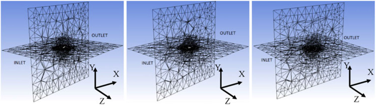
The faces forming the wing were attributed with the impervious wall boundary condition. Dynamic meshing technique was used in the present study of simulating flapping wing involving moving body. This approach always raises an apprehension of distortion of grids in the space between the sphere and the cubic far-field and affecting the prescribed boundary conditions at the inlet and outlet. This concern was addressed by choosing a larger cubic far-field domain. Two orthogonal longitudinal planes (XY and XZ planes) bisecting the computational domain were created and the shape of the deformed mesh during supination, mean and pronation phase of the flapping was plotted. Snapshots of the plots showing the mesh in the two planes and outlet are shown in Fig. 2. It was observed that while the quality of the mesh near the spherical sub-domain exhibited deformation, the quality of mesh near the inlet and outlet were not affected. Hence the dynamic mesh did not affect the boundary conditions during the simulation.
Grid during different wing positions (a) Pronation (b) Mean (c) Supination.

This apart, the maximum allowable skewness of the grid in the dynamic meshing setting of the solver was limited to 0.8. Laplacian smoothening operator was applied to the quadrilateral grid to reposition the nodes. This resulted in a check on the distortion of grids at each instance of wings’ movement and ensuring that the quality of the grid was acceptable. Visual impression from Fig. 2 is that the meshes at certain locations of the outer zone of the computational domain are highly skewed. However, upon carrying out the grid quality check throughout the period of the flapping cycle, it was observed that the skewness in these finite volumes ranged between 0.6 to 0.75, grid Jacobian was in the range of 0.5 to 0.6 and volume skewness ranged between 0.7 to 0.8. In light of these statistics of grid quality, the grid was considered to be acceptable for the envisaged simulation with dynamic meshing technique.
2.3 Verification and validation studies
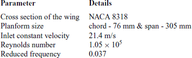
Usage of Ansys Fluent is reported in literature for analysing flow past flapping foils. Gharali et al (Reference Gharali and Johnson35) have used Ansys Fluent to investigate flapping foil under unsteady free stream conditions. Rezaei and Taha(Reference Razaei and Taha36) employed Ansys Fluent to study the lift frequency response of pitching airfoil and identify the effect of viscosity on the effect created by the airfoil kinematics. Taha and Rezaei(Reference Taha and Razaei37) reported studies on the unsteady viscous lift force response using triple deck theory. In line with these literature, verification and validation of the numerical model were carried out prior to employing the numerical model for investigating the sensitivity of the planform shapes to the gusty condition. The verification and validation studies aimed at ascertaining the accuracy and reliability of the present numerical model to handle simulation involving moving boundaries. These studies included domain, grid and time-step independence studies. The accuracy of the numerical model was ascertained by comparing the numerical predictions with the experimental observations(Reference Fejtek and Nehera38). Experiments were conducted in an open-return wind tunnel with a closed working section of 61 cm × 91 cm. A scotch yoke mechanism in combination with a rack and spur gear flapped the wing sinusoidally. The flapping mechanism was operated using a chain drive coupled to a 25 W induction motor. The wing was mounted on a steel sting in such a way that the hinge line was level with the surface of the wind tunnel floor. The sting was strain-gauged and the forces were measured using a Wheatstone bridge circuit. A high-speed A/D converter was used to scan the outputs of the Wheatstone bridge and forces were calculated by resolving the measured forces into the horizontal plane perpendicular and parallel to the direction of the free stream. The flapping kinematics for the experimental studies was simple symmetric flapping with flapping amplitude of 45 deg. and flapping frequency of 3.3 Hz. Details of the case study parameters like wing cross-sectional geometry, kinematics, and inflow condition are tabulated in Table 2.
Details of the wing and flow parameters

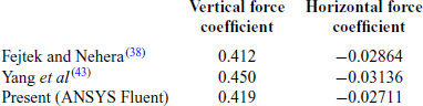
The flapping kinematics and the inflow conditions reported in the experimental benchmark studies translate to the variation of the angle of attack in the range of −5.63º to +5.63º at the mid-span location of the wing during a flapping cycle. Instantaneous vertical and horizontal forces generated by the wing during one flapping cycle can be reasonably derived based on the variation of the angle of attack and resolution of the corresponding static lift and drag forces in the vector directions parallel and perpendicular to the inflow velocity vector. Force coefficients were computed from the surface integrals of the pressure acting on the wing, resolving them in horizontal (along X-axis) and vertical (along Y-axis) direction and non-dimensionalising them by dynamic force based on the constant free stream velocity and wing’s planform area. NACA 8314, which is a cambered airfoil, is used for general aviation(Reference Abbott and Sherman39) and morphing UAV applications(Reference Prisacariu and Rau40). Fritz and Long(Reference Fritz and Long41) have reported its usage for flapping wing application. The static aerodynamic characteristics of the profile are reported by Jacob and Sherman(Reference Jacobs and Sherman42). Domain independence studies were carried out by considering five domains with the extent of domain size along X, Y, and Z axis ranging from 900c to 2500c. Here, c is the mean chord of the flapping foil. Grid independence studies were carried out by considering five grids with ds/c ranging from 0.01 to 0.1 with a total number of nodes ranging from 36,800 to 7,70,000, respectively. Here, ds is the elemental equally sized cell length of the side of the elemental quadrilateral grids, which covered the surface of the wing. Time-step independence studies were carried out by considering five-time step sizes ranging from T/25 to T/1000. Here, T is the period of one flapping cycle. From these independence studies, a domain with an extension of [−1050,1050] along X, Y, and Z axis, a grid with ds/c of 0.025 and 2.15 × 10⁵ nodes and a time-step size of T/500 was chosen. The solver exhibited transients in the estimates of the forces generated due to the flapping wing. In order to address this aspect in the numerical simulation, time-synchronous averaged force coefficients were calculated. The present simulations are carried out using a laminar computational model. Yang et al.(Reference Yang, Bifeng, Wenping and Liguang43) had carried out validation of their numerical models with Spalart-Allmaras turbulence modelling for the same experimental benchmark case(Reference Fejtek and Nehera38). A comparative plot of the present predictions with the benchmark experimental data(Reference Fejtek and Nehera38) and numerical predictions by Yang et al.(Reference Yang, Bifeng, Wenping and Liguang43) are shown in Fig. 3. Error bands in the experimental data have also been indicated in the comparative plots. In spite of usage of turbulence model in their numerical method, Yang et al.(Reference Yang, Bifeng, Wenping and Liguang43) reported deviations between the experimental data and numerical predictions during pronation and supination. For the experimental data, four active arm Wheatstone bridge circuit was used and a 10 Hz cut-off low pass filter was applied to filter out the noise and vibration-induced input signals(Reference Fejtek and Nehera38). Comparative plots of the instantaneous vertical and horizontal force coefficients are shown in Fig. 3(a) and (b), respectively, and cycle-averaged values are provided in Table 3.
Instantaneous vertical and horizontal force coefficients versus non-dimensional time. (a) Vertical force coefficient (b) Horizontal force coefficient.

Flapping cycle averaged vertical and horizontal force coefficients

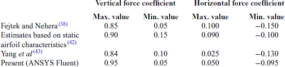
Comparison of the maximum and minimum instantaneous force coefficients based on the experiments(Reference Fejtek and Nehera38), estimates based on the static airfoil characteristics of NACA 8318(Reference Jacobs and Sherman42), numerical predictions(Reference Yang, Bifeng, Wenping and Liguang43) and the present approach are shown in Table 4.
Instantaneous vertical and horizontal force coefficients

The experimental results, which have been compared with the present laminar numerical simulation, corresponding to a Reynolds number of 1 × 10⁵. Differences between the experimental and numerically predicted instantaneous force coefficients are observed during the pronation and supination. These aspects raise concern on the choice of benchmark case and reliability of the numerical solver. In spite of these deviations between the experimental data and the numerical predictions, the trends of variation of the instantaneous force coefficients are similar in nature. It was observed that the predicted flapping cycle averaged vertical and horizontal force coefficient values from the present method were within 5% of the reference benchmark case. In light of these facts, the present numerical approach was considered reliable. These validation studies further confirmed that the present methodology could handle unsteady flow physics across a flapping wing with moving boundaries and constant frontal inflow condition. Simulation Reynolds number in the comparative studies, reported in this paper, was maintained within 104. Hence the usage of laminar models was justified.
2.4 Wing planform shapes
Wings with five different planform shapes, as shown in Fig. 4(a)–(e), were considered. Cross section of the wing was a flat plate with a constant thickness of 0.3 mm with chord length varying according to the planform shape. Among these five planform shapes, three wing shapes i.e. rectangular, triangular and elliptical wings [Fig. 4(a)–(c)] were symmetric about the spanwise axis passing through their root mid-chord. The other two wings i.e. semi-ellipse and inverse semi-ellipse [Fig. 4(d) & (e)], were asymmetric about the spanwise axis passing through their root mid-chord. Wingspan (155 mm) i.e. distances between the root chord to the wing tip and wing area (11,625 mm2) was kept constant to maintain same aspect ratio for all the wings.
Symmetric and asymmetric wing planforms.

2.5 Wing kinematics
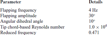
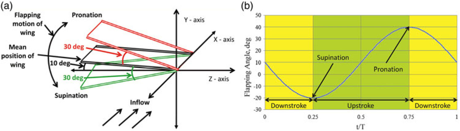
Generally, ornithopters use a combination of flapping and pitching and entomopters use a combination of flapping, pitching, and sweeping kinematics for flying. However, before studying the fluid dynamics of such complex flapping kinematics, it is imperative to first understand the fluid dynamics of the fundamental canonical forms of flapping kinematics and then graduate to complexities at next level of study. Hence, the present study is limited to one such canonical form of flapping i.e. asymmetric 1 DoF flapping. The wing is allowed to perform a simple flapping movement about X-axis. The mean position of flapping lies at an angular dihedral of 10º from the Z-axis (looking clock-wise from upwind). This angular dihedral of the mean position of wing results in the generation of a positive mean vertical force during flapping of the wing. In absence of this angular dihedral asymmetry, i.e. if the mean position of the wing coinciding with Z-axis, the vertical force produced during the upstroke and downstroke would nullify each other and the net vertical force generated during one flapping cycle would be zero. This study provided a baseline context before higher degrees of complex flapping kinematics and unsteady aerodynamics associated with real ornithopters and entomopters are attempted. This asymmetric kinematics has been reported by Hong and Altman(Reference Hong and Altman44). Details of the kinematic parameters and flow conditions are provided in Table 5.
Details of the kinematic parameters and flow conditions

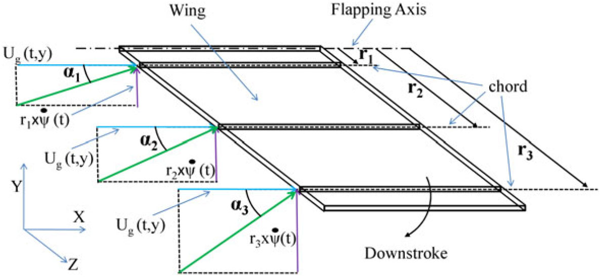
Even though the kinematics is a canonical form of asymmetric 1 DoF flapping, due to gusty shear inflow and spanwise variation of velocity vector hitting the wing, description of the angle of attack becomes complicated. Spanwise variation of the inflow velocity vector for the wing with rectangular planform shape is shown in Fig. 5.
Spanwise variation of the inflow velocity vector of a rectangular wing.

The angle of attack, α is calculated using the following expression:
 $$
\alpha ={{\rm tan}}^{{\rm -1}}\left(\frac{{{\rm U}}_{{\rm G}}{\rm (t,y)}}{{\rm r\times }\mathop \psi \limits^. {\rm (t)}}\right)$$
Here, UG(t, y) is the spatiotemporal gust frontal velocity vector and r is the spanwise radial distance of any cross-section of the wing from the flapping axis. As observed from the expression of the angle of attack, it varies along the span as well as at each instant of flapping due to gusty inflow condition. Hence, the variation of flapping angle, ψ, is reported instead of angle of attack. Wing kinematics and variation of the flapping angle, ψ, during one flapping cycle are shown in Fig. 6. The frontal inflow is along the X-axis. In order to simulate the kinematics, a User Defined Function (UDF) sub-routine was written. Different phases of the flapping cycle involve the wing flapping from the mean position, downward travel, supination, upward travel, pronation and then return back to the mean position. There is no dwell during the pronation or supination of the wing.
Wing kinematics. (a) Wing motion (b) Variation of flapping angle.

2.6 Gust model
Harland and Jacob(Reference Harland and Jacob45) have reported different models for representing unsteady gusts. Most commonly adopted temporally varying gust models amongst them are sharp-edged gust and oscillatory gust models. However, in a real-life gust, apart from the temporally varying component, there also exist spatial gradients or wind shear. Hence, we propose a simple gust model with a single gust frequency and a 1-D spatial gradient superimposed over a non-zero mean free stream velocity. The equation is as follows:
 $$
\frac{U_G}{U_w}=\frac{U_{\infty }}{U_w}+\left(\frac{U_g}{U_w}\right)sin\left(2\pi \frac{f_g}{f_w}t\right){\pm}\left(\frac{V_{grad}}{U_w}\right)y
$$
Here, UG is the gust velocity in m/s, U∞ is mean free stream velocity in m/s, Ug is gust amplitude in m/s, Vgrad is the linear velocity gradient along the Y-axis in m/s per m, fg is gust frequency in Hz, fw is the wing flapping frequency in Hz, y is spatial dimension along Y-axis in m and t is time in second. The velocity components were non-dimensionalised using Uw, the root mean square average flapping velocity at the wing tip in m/s. The nature of spatiotemporal gust model and velocity vector at the inlet is shown in Fig. 7(a) and (b) respectively. For the present study, Ug was considered to be 10% of Uw. The ratio of fg to fg was 0.1. Spatial velocity gradient, i.e. ratio of Vgrad to Uw, was considered to be 10. U∞ was considered as 2 m/s to confine the fluid dynamic parameter to laminar and unsteady state. Considering the free stream velocity to 2 m/s translated to simulation Re of 1.0 × 10⁴ (i.e. laminar state), and reduced frequency, k of 0.471 (i.e. unsteady state) based on the average chord of the wing.
Spatio-temporal gust model. (a) Frontal shear gust profile at inlet, (b) Velocity vectors representing shear gust profile at different instances of Tg at inlet.

3.0 RESULTS AND DISCUSSIONS
Baseline simulations were carried out for a constant velocity inflow condition for all the five wings. Subsequently, frontal spatiotemporally varying gusty inflow condition was specified. Findings were analysed by comparing the force patterns and carrying out the numerical flow visualization. Findings are reported in the following sub-sections.
3.1 Force patterns
Three approaches were adopted to compare force patterns and ascertain gust sensitivity of the five wings with different wing planform shapes. These approaches included a comparison of differences in the instantaneous force coefficients for different inflow conditions over a gust cycle, ordinal score based on gust cycle averaged force coefficients, and phase space diagrams.
3.1.1 Variation in instantaneous force coefficients over a gust cycle
As mentioned earlier, simulations were carried out and instantaneous force coefficient in vertical and horizontal directions with constant (CVC and CHC) and gusty (CVG and CHG) inflow conditions were computed. The expressions to calculate these force coefficients are as follows:
 $$
{{\rm C}}_{{\rm VC}}=\frac{{{\rm F}}_{{\rm VC}}}{\frac{1}{2}{\rm \times }{\rho} {\rm \times }{{\rm A}}_{{\rm wing}}{\rm \times }{{\rm U}}_{\infty }},\quad {{\rm C}}_{{\rm HC}}=\frac{{{\rm F}}_{{\rm HC}}}{\frac{1}{2}{\rm \times }{\rho } {\rm \times }{{\rm A}}_{{\rm wing}}{\rm \times }{{\rm U}}_{\infty }},\quad {{\rm C}}_{{\rm VG}}=\frac{{{\rm F}}_{{\rm VG}}}{\frac{1}{2}{\rm \times }{\rho } {\rm \times }{{\rm A}}_{{\rm wing}}{\rm \times }{{\rm U}}_{\infty }} \& \\
{{\rm C}}_{{\rm HG}}=\frac{{{\rm F}}_{{\rm HG}}}{\frac{1}{2}{\rm \times }{\rho} {\rm \times }{{\rm A}}_{{\rm wing}}{\rm \times }{{\rm U}}_{\infty }}
$$
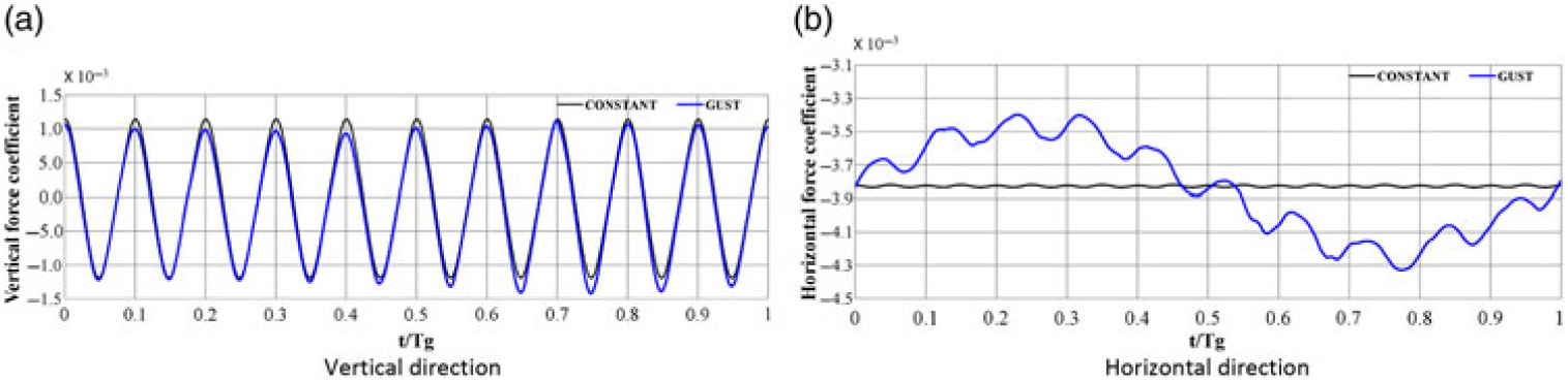
Here, Awing is wing planform area, U∞ is free-stream velocity and FVC, FHC, FVG, and FHG are vertical and horizontal forces generated by the wing with constant and gusty inflow conditions respectively. Temporal variation in the force coefficients for a rectangular wing is shown in Fig. 8(a) and (b). Similar patterns were observed for other four wings with triangle, elliptical, semi-elliptical, and inverse semi-elliptical planform shape.
Temporal variation in force coefficient for a wing with rectangular planform shape. (a) Vertical direction (b) Horizontal direction.

In order to assess the effect of gust on wings with different planform shapes, differences of the instantaneous force coefficients in vertical and horizontal directions with different inflow conditions were compared. The expression to calculate these differences are shown below:
 $$
\textrm{Difference of force coefficients in the vertical direction},\ \Delta {\rm C}{}_{\rm V} = {{\rm C}}_{{\rm VG}}-{{\rm C}}_{{\rm VC}}$$
 $$
\textrm{Difference of force coefficients in the horizontal direction,}\ \Delta {\rm C}{}_{\rm H} = {{\rm C}}_{{\rm HG}}-{{\rm C}}_{{\rm HC}}
$$
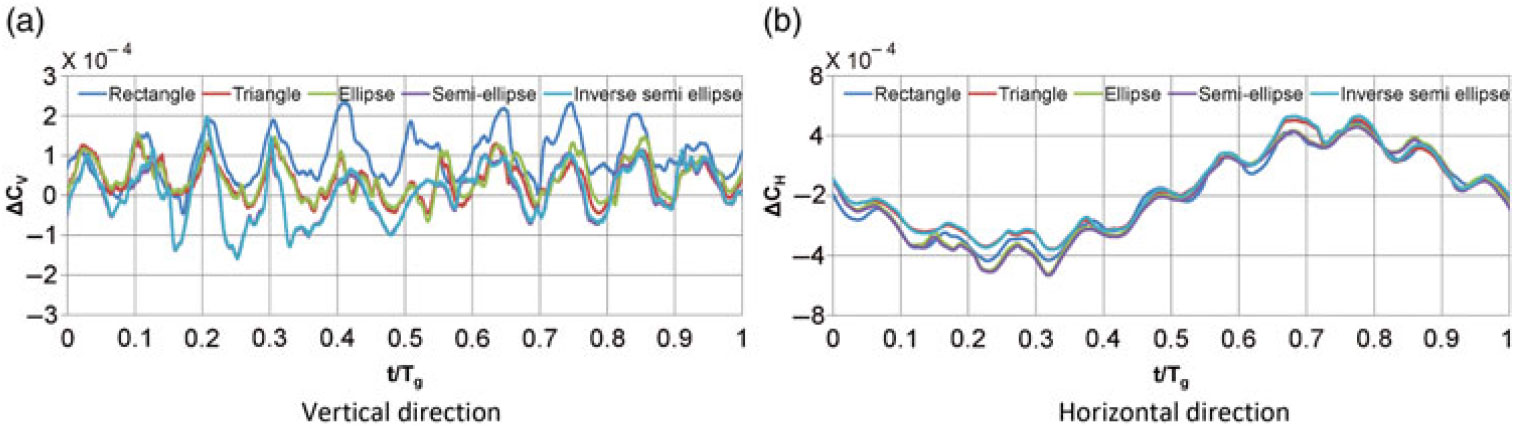
Instantaneous variations of the differences in the force coefficients for all the five wing planforms are shown in Fig. 9(a) and (b). It was observed that gust affected the instantaneous vertical and horizontal force coefficients throughout the gust cycle.
Temporal variation in the difference in instantaneous force coefficients for all wing planforms. (a) Vertical direction (b) Horizontal direction.

3.1.2 Ordinal scores for wings based on gust cycled average force coefficients
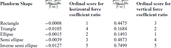
In order to have an overall assessment of the sensitivity of the wing planforms, ordinal scores were allocated to the wing planform shapes. The ordinal score is a well-proven methodology in statistics. The scores are assigned to the objects to determine the relative extent to which they possess a certain characteristic. It helps in identifying whether the object has a superior or inferior characteristic as compared to the other object. An ordinal score of 1 corresponds to the least change in the gust averaged force coefficients. An ordinal score of 5 corresponds to the higher change in the force coefficients. In order to have an overall assessment of the sensitivity, the ordinal scores based on the horizontal and vertical force coefficients for the respective planform shapes were summed up.
For assigning ordinal scores to the wings, gust cycle averaged force coefficients were calculated for all the wings with different planform shapes. One gust cycle consisted of 10 flapping cycles. In the present study, three gust cycles were simulated for each wing. The solver exhibited transients during first few flapping cycles of the first gust cycle. Hence, time-synchronous averaged force coefficients based on the second and third gust cycle were considered. To calculate the average force coefficients for the constant inflow condition, the same duration of the simulation, which was considered for calculating the gust cycle averaged force coefficients, was considered. Details of the findings are summarised in Table 6.
Force coefficient ratios and their ordinal scores

From the findings, it was observed that the effect of a gust on the horizontal force pattern was less for wings with rectangular and elliptical wing planform. The effect of gust was less for elliptical and triangular wings when compared in terms of vertical force pattern. Accordingly, ordinal scores were separately assigned to the wings with different planform shapes based on the differences in the horizontal and vertical force coefficient for constant and gusty inflow conditions and were summed up. It was observed that the total ordinal score for the respective wing planform shapes summed as 4 for a wing with rectangular planform shape, 6 for a wing with triangular planform shape, 3 for a wing with elliptical planform shape, 7 for wing with semi-elliptical planform shape and 10 for a wing with inverse semi-elliptical planform shape. Hence, the order of sensitivity of wings to an incoming spatiotemporal gust is elliptical, rectangular, triangular, semi-elliptical and inverse semi-elliptical wing planform shape in ascending manner of their sensitivity to gust. The order is from least sensitive to the most sensitive shape of wing planform. This indicated that the elliptical wing was least susceptible to a spatiotemporal wind gust, while inverse semi-elliptical wing’s performance was most affected by a gusty condition.
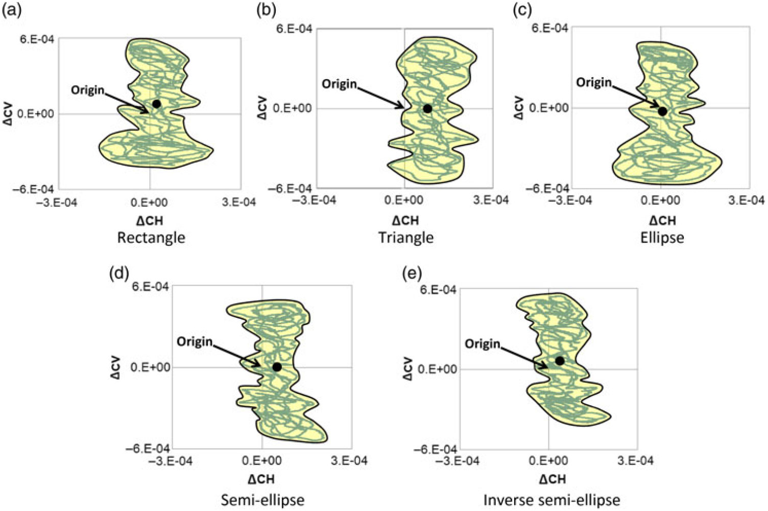
Phase space diagrams. (a) Rectangle (b) Triangle (c) Ellipse (d) Semi-ellipse (c) Inverse semi-ellipse.

3.1.3 Phase space diagrams
In order to further study the effect of gust on the force patterns generated by wings with different planform shapes, phase space diagrams based on the instantaneous differences of force coefficients were plotted. The instantaneous difference in horizontal force coefficient with constant and gusty inflow conditions was plotted on the abscissa. The instantaneous difference in vertical force coefficient with constant and gusty inflow conditions was plotted on the ordinate. The diagrams are shown in Fig. 10(a)–(e). The area bounded under the phase space diagram are shown by shading so as to mutually differentiate them. The centroid of the bounded area have also been marked and shown for respective phase space plots. Nearness of the centroid vis-à-vis the origin of the phase space diagram is an indicator of the sensitivity of the wing to the inflow condition. If the centroid is at the origin, it indicates that the overall effect of the instantaneous differences in the force coefficients due to different inflow condition over a gust cycle is neutral. It is observed from the plots that for the wing with the elliptical wing, the centroid was closest to the origin of the plot. The centroid for the inverse semi-elliptical wing was relatively furthest. This implied that the elliptical wing was least sensitive and inverse semi-elliptical wing was more sensitive to the gusty inflow condition. This observation was also in line with the sensitivity ranking arrived by ordinal score approach.
3.2 Numerical flow visualization
Quantitative and qualitative findings of the effect of planform shapes on the force generation pattern of flapping wings were reported in the previous section. This section reports the numerical flow visualization of the flow field in the vicinity of the wings with different planform shapes. Three approaches viz. vortex structure identification based on Q criteria, surface static pressure contour plots, and plots of Lagrangian Coherent Structure (LCS) along the spanwise axis of the wing have been adopted. Variation of the differences in instantaneous vertical force coefficient due to different inflow conditions was observed throughout the gust cycle. Variation of the differences in instantaneous horizontal force coefficient due to different inflow conditions was lowest and highest during t/Tg = 0.2 – 0.35 and t/Tg = 0.65 – 0.8 respectively. Hence the vortex structures, surface pressure plots and LCS at t/Tg = 0.30 and t/Tg = 0.75 were plotted. The downstroke and upstroke angles of attack corresponding to these two instants are 17.4° and −17.4° respectively. They are the maximum and minimum angles of attack occurring during the flapping cycle. These approaches helped in distinguishing the fluid dynamics of wings with different planform shape under constant and gusty inflow conditions.
3.2.1 Vortex patterns based on Q-criteria
3D vortical structures were visualised by employing the Q-criterion. It is the second invariant of the velocity gradient tensor. It represents the local balance between shear strain rate and vorticity magnitude and identifies vortices as areas in the flow field where the vorticity magnitude is greater than the magnitude of rate-of-strain i.e. Q > 0. Q is calculated using Eq. (Reference Warkentin and Delaurier6).
 $$
{\rm Q=}\frac{1}{2}\left[{\left\|{\Omega }_{{\rm ij}}\right\|}^{2}-{\left\|{{\rm S}}_{{\rm ij}}\right\|}^{2}\right]$$
Here  ${\Omega }_{ij}=\frac{1}{2}\left(\frac{\partial u_i}{\partial x_j}-\frac{\partial u_j}{\partial x_i}\right){\rm \ and}{{\rm \ S}}_{ij}=\frac{1}{2}\left(\frac{\partial u_i}{\partial x_j}+\frac{\partial u_j}{\partial x_i}\right)$
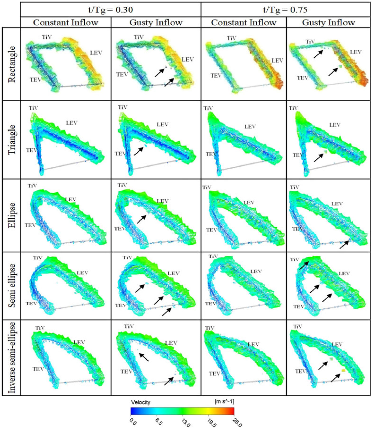
Vortical structures like leading-edge vortex (LEV), trailing edge vortex (TEV) and tip vortex (TiV) at t/Tg=0.30 and t/Tg=0.75 were plotted. For ease of identifying the inflow direction, leading edge (LE) and trailing edge (TE) are labelled. The flow visualisation plots are shown in Fig. 11. Vortical structures were rendered with velocity magnitudes to distinguish the structures.
Vortex patterns based on Q-criteria in the vicinity of different wings.

At t/Tg=0.30, the wing undergoes downstroke and is at its mean position. The LEV, TEV and TiV are observed to be attached on the suction surface of the wing. At t/Tg=0.75, the wing undergoes upstroke and is at its mean position. The LEV, TEV and TiV are observed to be attached on the pressure surface of the wing. A close study of the plots revealed that there exists a difference in the primary vortex patterns at the edge of the wings with constant and gusty inflow conditions. Secondary vortex patterns were observed in the vicinity of primary circulation about the wing for gusty inflow condition near the leading edge for the same instance of time. Presence of these secondary flow structures and their shedding in the wake was advanced due to the gusty inflow condition. These secondary blobs of vortices are mainly observed (shown with arrows in Fig. 11) for wings with rectangular, triangular, semi-elliptical and inverse semi-elliptical planforms as compared to the elliptical wing.
From these observations, it was inferred that the effect of gust on the elliptically shaped wing was less as compared to the other four wings considered in the present study. It was further observed that the tip vortex structures of the elliptically shaped wing were similar for constant and gusty inflow conditions. For the other four wings with sharp corners at the tip, the TiVs formed for constant and gusty inflow were different. This difference was primarily attributed to the fact that the elliptically shaped wing had a continuous and smooth wing boundary edge, whereas all the other wings had sharp corners at their peripheral boundaries. These sharp corners in the peripheral boundaries of the wings became pockets of sensitive zones. Flow pattern at these geometric discontinuities differed for the constant and gusty inflow in these zones. These differences in the flow patterns translated into the differences observed in the forces occurring during flapping of these wings with different inflow condition and justified the quantitative inferences made in the previous section. These differences become more pronounced during the stroke reversal and hence translate into the difference in the instantaneous force coefficients.
Surface pressure contours over suction and pressure surfaces of different wings.

Lagrangian Coherent Structures along the spanwise axis of different wings.

3.2.2 Surface static pressure contours
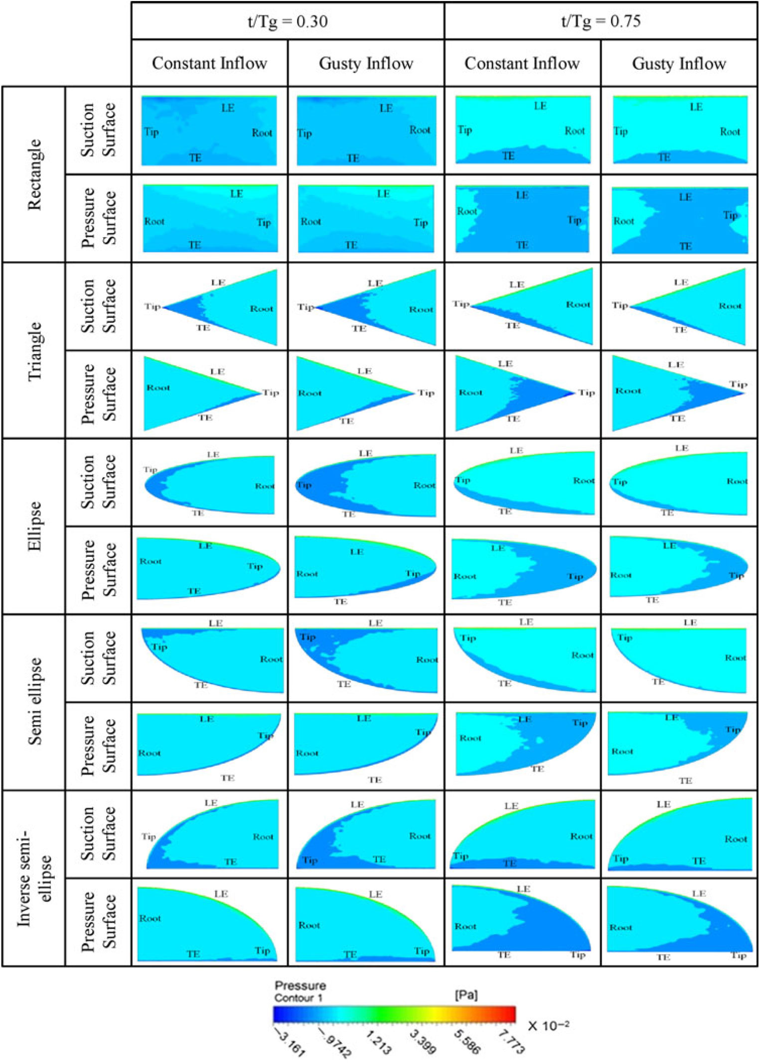
While numerical flow visualisation of the vortex structures in the vicinity of the moving wings revealed an insight into the vortical structures occurring in the vicinity of the wing, the surface static pressure contours represented the effect of the vortex structures on the wing. Surface integrals of these pressure forces occurring over the suction and pressure surface of the wing along X and Y axis were carried out to compute the horizontal and vertical forces generated by the wing at that instance of flapping. Hence, comparative study of the surface static pressure contours over the flapping wing with constant and gusty inflow conditions helped us to physically interpret the differences in force patterns. The contours are shown in Fig. 12.
Differences in the pressure distribution over the wing surfaces are clearly visible for constant and gusty inflow conditions. The differences in pressure contours predominantly occur at the out-board suction and pressure surfaces of the wing for t/Tg=0.30 and t/Tg=0.75, respectively. When compared with the elliptically shaped wing, the differences were distinct and prominent for the other four wings considered in the present study. Also, the zone of influence over the wing surfaces was observed to be more for the gusty inflow condition. It was observed that the low static pressure zones over the wing had increased due to the gusty inflow condition. However, as mentioned, these differences in the pressure zones were observed to be less for the elliptical wing with constant and gusty inflow condition. The effect was observed to be more for the semi-elliptical and inverse semi-elliptical wing. For the rectangular and triangular wings, the effect was observed to be moderate during the two temporal instances. These observations reinforced the inferences made in the previous section that the elliptically shaped wing exhibited less sensitivity to the frontal gusty inflow condition as compared to the wings with rectangular, triangular, semi-elliptical and inverse semi-elliptical planform shapes.
3.2.3 Lagrangian coherent structures along spanwise axis
Vortex structures near the flapping wings at t/Tg=0.30 and t/Tg=0.75 occurring in the plane passing through longitudinal spanwise axis were visualised by computing the Lagrangian Coherent Structures (LCS). They are the ridges of Finite-Time Lyapunov Exponent (FTLE) field and are shown in Fig. 13. The FTLE measures the maximum rate of separation around a certain location in the fluid domain(Reference Rockwood, Huang and Green46). Flow map of particles over an integration time, T, is initially computed. Then the Cauchy-Green strain tensor is constructed from the spatial gradient of the flow map. Subsequently, the FTLE field is computed from the maximum eigenvalue of the Cauchy-Green strain tensor. Detailed numerical formulations are reported by Srinidhi and Vengadesan(Reference Srinidhi and Vengadesan47). The time period of one gust cycle was chosen as the integration time, T, for computing the FTLE in the present study. For t/Tg=0.30 and t/Tg=0.75, the LCS was observed over the suction and pressure surfaces of the wing, respectively. Root and tip vortices were prominently visible. The intensity of the LCS along the span was the representative of the spanwise transport of the fluid particles.
While the structure of LCS was observed to be similar in nature, the intensity varies from constant inflow to gusty inflow at both the temporal instances viz. t/Tg=0.30 and t/Tg=0.75. The intensity was observed to be more prominent for wing with semi-elliptical and inverse semi-elliptical planform shapes. This implied that flow patterns occurring in the vicinity of these two wings were affected more due to the gusty inflow condition. Differences in the intensity of LCS for the wings with rectangular and triangular planform shapes were observed to be slightly less as compared with the two former wings. The intensity of LCS for the elliptical wing was marginally different. From these observations, it was inferred that the flow along the spanwise axis for the elliptical wing was affected least and that for semi-elliptical and inverse semi-elliptical wing were affected most. The flows along the spanwise axis of the rectangular and triangular wing were affected moderately. These observations supported the quantitative observations made in the previous sections based on the force patterns.
4.0 CONCLUSIONS
Sensitivity assessment of five wing planforms to a spatiotemporally varying frontal gusty inflow has been reported in the present paper. The gust model consisted of a single frequency temporally fluctuating velocity term, a 1D frontal velocity gradient term and a non-zero mean velocity. A canonical form of flapping kinematics i.e. asymmetric 1 degree of freedom flapping (DoF) kinematics was considered. Findings were analyzed quantitatively by comparing the differences in the instantaneous and gust cycle averaged vertical and horizontal force coefficients, ordinal scores, and phase space diagrams. Qualitative comparisons were made based on visualization of vortex structures using Q-criteria, surface static pressure contour plots and visualization of spanwise flow features using LCS. Studies revealed that the elliptical wing exhibited the least sensitivity to the frontal gusty inflow profile as compared to the other wing planform shapes. Even though the present study was limited to a canonical case of 1 DoF asymmetric flapping kinematics and a specific case of frontal gusty inflow condition, the finding that elliptical wing is relatively less sensitive to gust ratified the fact that many natural flyers like forest raptors, non-migratory passerines, pheasants and partridges have adopted elliptical wing planforms for efficient flying.