2 Formulation and linear stability

The two-dimensional modified Rayleigh–Bénard convection (MRBC) model filters out fast gravity waves and hence represents a projection of the primitive equations onto the slow manifold. As a result, the model is suitable for studying strongly driven systems in which gravity wave frequencies are high and the simulation of the primitive equations prohibitively expensive. In two dimensions the dimensionless model equations take the form (Xie et al. Reference Xie, Knobloch, Miquel and Julien2017)

(2.1a ) $$\begin{eqnarray}\displaystyle \frac{1}{\mathit{Sc}}\left[\frac{\unicode[STIX]{x2202}}{\unicode[STIX]{x2202}t}\unicode[STIX]{x1D6FB}^{2}\unicode[STIX]{x1D713}+{\mathcal{J}}(\unicode[STIX]{x1D713},\unicode[STIX]{x1D6FB}^{2}\unicode[STIX]{x1D713})\right] & = & \displaystyle -\frac{\unicode[STIX]{x2202}S}{\unicode[STIX]{x2202}x}+(\unicode[STIX]{x0394}^{-1}\unicode[STIX]{x2202}_{xx}+\unicode[STIX]{x1D6FB}^{4})\unicode[STIX]{x1D713},\end{eqnarray}$$

(2.1b ) $$\begin{eqnarray}\displaystyle \frac{\unicode[STIX]{x2202}}{\unicode[STIX]{x2202}t}S+{\mathcal{J}}(\unicode[STIX]{x1D713},S)+\mathit{Ra}\frac{\unicode[STIX]{x2202}\unicode[STIX]{x1D713}}{\unicode[STIX]{x2202}x} & = & \displaystyle \unicode[STIX]{x1D6FB}^{2}S.\end{eqnarray}$$

$\unicode[STIX]{x1D713}$

$S$

${\mathcal{J}}(a,b)\equiv a_{x}b_{z}-a_{z}b_{x}$

$\unicode[STIX]{x0394}^{-1}$

The dimensionless quantities present in (2.1) are defined as follows:

(2.2a-d ) $$\begin{eqnarray}t=\frac{\unicode[STIX]{x1D705}_{S}}{d^{2}}t^{\ast },\quad (x,\,z)=\frac{1}{d}(x^{\ast },\,z^{\ast }),\quad \unicode[STIX]{x1D713}=\frac{1}{\unicode[STIX]{x1D705}_{S}}\unicode[STIX]{x1D713}^{\ast }\quad \text{and}\quad S=\frac{\mathit{R}_{\unicode[STIX]{x1D70C}}\unicode[STIX]{x1D70F}}{\unicode[STIX]{x1D6FD}_{S}d}S^{\ast },\end{eqnarray}$$

where $^{\ast }$ indicates dimensional quantities and

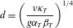(2.3) $$\begin{eqnarray}d=\left(\frac{\unicode[STIX]{x1D708}\unicode[STIX]{x1D705}_{T}}{g\unicode[STIX]{x1D6FC}_{T}\unicode[STIX]{x1D6FD}_{T}}\right)^{1/4}\end{eqnarray}$$

is the (dimensional) natural finger scale.

The MRBC model describes salt-finger convection in the limit $\unicode[STIX]{x1D70F}\rightarrow 0$ , $\mathit{R}_{\unicode[STIX]{x1D70C}}\rightarrow \infty$ , a regime described by two independent dimensionless parameters instead of the usual three, the Prandtl number $\mathit{Pr}\equiv \unicode[STIX]{x1D708}/\unicode[STIX]{x1D705}_{T}$ , the density ratio $\mathit{R}_{\unicode[STIX]{x1D70C}}\equiv \unicode[STIX]{x1D6FC}_{T}\unicode[STIX]{x1D6FD}_{T}/(\unicode[STIX]{x1D6FC}_{S}\unicode[STIX]{x1D6FD}_{S})$ and the diffusivity ratio $\unicode[STIX]{x1D70F}\equiv \unicode[STIX]{x1D705}_{S}/\unicode[STIX]{x1D705}_{T}$ . The model assumes that these two remaining parameters, the Rayleigh ratio

(2.4) $$\begin{eqnarray}\mathit{Ra}\equiv \frac{1}{\mathit{R}_{\unicode[STIX]{x1D70C}}\unicode[STIX]{x1D70F}}=\frac{\mathit{Ra}_{S}}{\mathit{Ra}_{T}}\end{eqnarray}$$

and the Schmidt number $\mathit{Sc}\equiv \unicode[STIX]{x1D708}/\unicode[STIX]{x1D705}_{S}$ , both remain of order one. Here

(2.5a,b ) $$\begin{eqnarray}\mathit{Ra}_{T}=\frac{g\unicode[STIX]{x1D6FC}_{T}\unicode[STIX]{x1D6FD}_{T}H^{4}}{\unicode[STIX]{x1D708}\unicode[STIX]{x1D705}_{T}}\quad \text{and}\quad \mathit{Ra}_{S}=\frac{g\unicode[STIX]{x1D6FC}_{S}\unicode[STIX]{x1D6FD}_{S}H^{4}}{\unicode[STIX]{x1D708}\unicode[STIX]{x1D705}_{S}}\end{eqnarray}$$

are the usual thermal and solutal Rayleigh numbers characterizing the stabilizing temperature and destabilizing salinity profiles. In these expressions $\unicode[STIX]{x1D6FC}_{T,S}$ are the expansion coefficients, $\unicode[STIX]{x1D705}_{T,S}$ are the diffusivities, $\unicode[STIX]{x1D6FD}_{T,S}$ are the background gradients, $g$ is the gravitational acceleration, $H$ is the layer depth and $\unicode[STIX]{x1D708}$ is the kinematic viscosity; the subscripts $T$ and $S$ denote temperature and salinity, respectively. When $\unicode[STIX]{x1D70F}$ is small, i.e. when the temperature field diffuses much more rapidly than salinity, the above regime corresponds to strong driving via an unstable salt stratification. In this regime the temperature field is slaved to the velocity field and may be eliminated from the governing equations via a systematic asymptotic expansion in the small parameter $\unicode[STIX]{x1D70F}$ (Xie et al. Reference Xie, Knobloch, Miquel and Julien2017). Equations (2.1) represent the leading-order description of the system to within $O(\unicode[STIX]{x1D70F})$ corrections.

To relate the intrinsic scale for salt-finger convection to the scale $d$ we substitute a normal mode ansatz of the form $(\unicode[STIX]{x1D713},S)=\text{e}^{\unicode[STIX]{x1D706}t+\text{i}(kx+mz)}(\unicode[STIX]{x1D713}_{0},S_{0})$ into (2.1), linearized around $S=\unicode[STIX]{x1D713}=0$ . We find that the linear growth rate $\unicode[STIX]{x1D706}$ satisfies

(2.6) $$\begin{eqnarray}\unicode[STIX]{x1D706}^{2}+\left[|\boldsymbol{k}|^{2}+\frac{\mathit{Sc}}{|\boldsymbol{k}|^{4}}(k^{2}+|\boldsymbol{k}|^{6})\right]\unicode[STIX]{x1D706}+\frac{\mathit{Sc}}{|\boldsymbol{k}|^{2}}(k^{2}+|\boldsymbol{k}|^{6}-\mathit{Ra}k^{2})=0,\end{eqnarray}$$

where $|\boldsymbol{k}|^{2}=k^{2}+m^{2}$ . This equation informs us that linear instability is present only when the last term is negative, i.e. when

(2.7) $$\begin{eqnarray}\mathit{Ra}>\mathit{Ra}(k,m)\equiv 1+\frac{|\boldsymbol{k}|^{6}}{k^{2}}.\end{eqnarray}$$

This condition is independent of $\mathit{Sc}$ and so applies even in the limit $\mathit{Sc}\rightarrow \infty$ appropriate for terrestrial oceans. The critical value of $\mathit{Ra}$ for linear instability is thus $\mathit{Ra}_{c}=1$ and the instability sets in with wavenumbers $(k,m)=(0,0)$ . In the following we find that the quantity ${\mathcal{R}}\equiv \mathit{Ra}-1$ provides a convenient measure of the distance from threshold, i.e. the supercriticality of the system. The positive (unstable) solution of (2.6) is

(2.8) $$\begin{eqnarray}\displaystyle \unicode[STIX]{x1D706} & = & \displaystyle \frac{1}{2}\left(\vphantom{\sqrt{\frac{1}{2}^{1}}}-\left[|\boldsymbol{k}|^{2}+\frac{\mathit{Sc}}{|\boldsymbol{k}|^{4}}(k^{2}+|\boldsymbol{k}|^{6})\right]\right.\nonumber\\ \displaystyle & & \displaystyle \left.+\,\sqrt{\left[|\boldsymbol{k}|^{2}+\frac{\mathit{ Sc }}{|\boldsymbol{k}|^{4}}(k^{2}+|\boldsymbol{k}|^{6})\right]^{2}-\frac{4\mathit{Sc }}{|\boldsymbol{k}|^{2}}(k^{2}+|\boldsymbol{k}|^{6}-\mathit{Ra}k^{2})}\right)\!,\end{eqnarray}$$

which reduces in the limit of $\mathit{Sc}\rightarrow \infty$ to the growth rate of the inertia-free salt-finger convection (IFSC) model derived by Xie et al. (Reference Xie, Knobloch, Miquel and Julien2017):

(2.9) $$\begin{eqnarray}\unicode[STIX]{x1D706}_{\mathit{IFSC}}=\mathit{Ra}\frac{k^{2}|\boldsymbol{k}|^{2}}{k^{2}+|\boldsymbol{k}|^{6}}-|\boldsymbol{k}|^{2}.\end{eqnarray}$$

When the supercriticality ${\mathcal{R}}$ is small, we find that the optimal growth rate behaves like

(2.10) $$\begin{eqnarray}\unicode[STIX]{x1D706}_{opt}=\frac{2}{3^{3/2}}{\mathcal{R}}^{3/2}+\text{h.o.t.},\end{eqnarray}$$

a quantity independent of $\mathit{Sc}$ to leading order, and hence identical to that for $\mathit{Sc}=\infty$ (Xie et al. Reference Xie, Knobloch, Miquel and Julien2017, equation (26b)), matching the small- $\mathit{Pr}$ result of Brown et al. (Reference Brown, Garaud and Stellmach2013, equation (B20)).

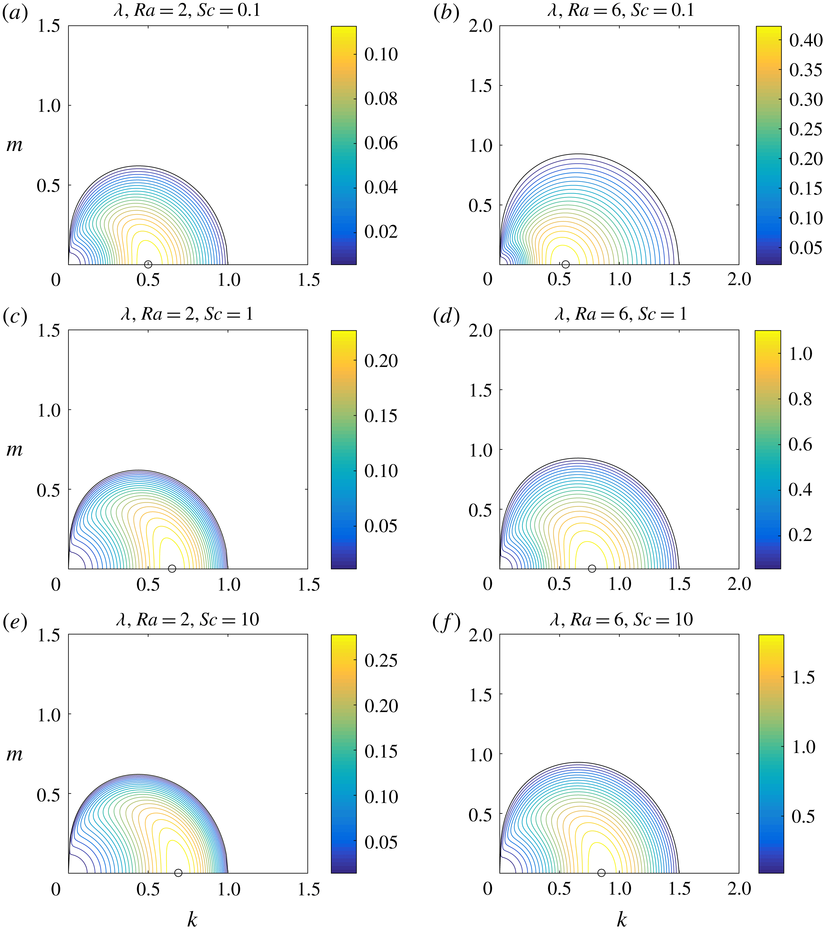
The linear growth rate $\unicode[STIX]{x1D706}(k,m)$ for $\mathit{Ra}=2$ and $\mathit{Ra}=6$ and three different values of $\mathit{Sc}$ is shown in figure 1. The figure highlights the anisotropic dependence of $\unicode[STIX]{x1D706}$ on $k$ and $m$ : for fixed $m$ , not too large, there exists an optimal $k$ that maximizes the growth rate, whereas when $k$ is fixed, an optimal $m$ exists for small $k$ , but for large $k$ the growth rate decreases monotonically with increasing $m$ . The sequence of plots in each column shows that the linear growth rate and the horizontal wavenumber $k$ of the most unstable mode increase with increasing $\mathit{Sc}$ , and we find that they reach a regular limit as $\mathit{Sc}\rightarrow \infty$ . The most unstable modes are the so-called elevator modes with $m=0$ . These modes are unstable within a band of horizontal wavenumbers $k$ that is well captured by the supercriticality ${\mathcal{R}}$ ,

(2.11) $$\begin{eqnarray}0<k^{4}<{\mathcal{R}},\end{eqnarray}$$

and are exact solutions of the nonlinear equations (2.1) with periodic boundary conditions in the vertical. However, in contrast to the IFSC model valid in the limit $\mathit{Sc}\rightarrow \infty$ , these modes are not directly involved in the saturation process. The reasons for this difference are elaborated below.

Figure 1.

Contour plots of the linear growth rate $\unicode[STIX]{x1D706}(k,m)$ of the MRBC model (2.1) defined in (2.8). Results for $\mathit{Ra}=2$ (a,c,e) and $\mathit{Ra}=6$ (b,d,f), respectively, for $\mathit{Sc}=0.1$ (a,b), $1$ (c,d) and $10$ (e,f). Only positive growth rates are shown. Circles mark the optimal wavenumbers: $0.50$ , $0.65$ and $0.68$ for $\mathit{Ra}=2$ and increasing $\mathit{Sc}$ , approaching the optimal wavenumber $0.69$ when $\mathit{Sc}=\infty$ ; and $0.55$ , $0.77$ and $0.85$ for $\mathit{Ra}=6$ and increasing $\mathit{Sc}$ , approaching the optimal wavenumber $0.88$ when $\mathit{Sc}=\infty$ .

3 Nonlinear simulations

In this section, we present two representative numerical simulations of the MRBC system (2.1). These use a Fourier pseudospectral method with $2/3$ dealiasing in space with resolution $512\times 512$ and a fourth-order explicit Runge–Kutta scheme in time with a fixed time step $5\times 10^{-3}$ in which the nonlinear terms are treated explicitly and linear terms implicitly using an integrating factor method. All calculations are initialized with small-amplitude random Gaussian fields whose amplitude determines the time required to reach saturation. The numerical results provide an empirical foundation for the theoretical development in later sections.

3.1 Simulation of the MRBC system with $\mathit{Ra}=6$ , $\mathit{Sc}=1$

We begin with the case $\mathit{Ra}=6$ , $\mathit{Sc}=1$ . This case corresponds to high-density-ratio simulations of two-dimensional salt-finger convection using primitive equations by Garaud & Brummell (Reference Garaud and Brummell2015), and therefore permits validation of the MRBC system. We present here the results of a simulation initialized with small homogeneous random perturbations $\unicode[STIX]{x1D713}$ and $S$ in a doubly periodic domain of size $L_{x}\times L_{z}\equiv 32l_{opt}\times 32l_{opt}$ . Here $l_{opt}=2\unicode[STIX]{x03C0}/k_{opt}$ is the wavelength of the fastest growing mode in the limit $\mathit{Sc}\rightarrow \infty$ , where

(3.1) $$\begin{eqnarray}k_{opt}^{4}={\textstyle \frac{1}{2}}(-2-\mathit{Ra}+\sqrt{\mathit{Ra }^{2}+8\mathit{Ra}}).\end{eqnarray}$$

In figure 2 we show the time evolution of the salinity potential energy $P_{S}$ , the salinity flux $F_{S}$ , the kinetic energy $K_{jet}$ in the jets that form and the fluctuation kinetic energy $K_{fluc}$ , defined as follows:

(3.2a ) $$\begin{eqnarray}\displaystyle P_{S} & = & \displaystyle \frac{1}{2A}\int S^{2}\,\text{d}x\,\text{d}z,\end{eqnarray}$$

(3.2b ) $$\begin{eqnarray}\displaystyle F_{S} & = & \displaystyle \frac{1}{A}\int \unicode[STIX]{x1D713}_{x}S\,\text{d}x\,\text{d}z,\end{eqnarray}$$

(3.2c ) $$\begin{eqnarray}\displaystyle K_{tot} & = & \displaystyle \frac{1}{2A}\int \left[(\unicode[STIX]{x1D713}_{x})^{2}+(\unicode[STIX]{x1D713}_{z})^{2}\right]\,\text{d}x\,\text{d}z,\end{eqnarray}$$

(3.2d ) $$\begin{eqnarray}\displaystyle K_{jet} & = & \displaystyle \frac{1}{2L_{z}}\int \left(\frac{1}{L_{x}}\int \unicode[STIX]{x1D713}_{z}\,\text{d}x\right)^{2}\,\text{d}z=\frac{1}{2L_{z}}\int \bar{U}^{2}\,\text{d}z,\end{eqnarray}$$

(3.2e ) $$\begin{eqnarray}\displaystyle K_{fluc} & = & \displaystyle K_{tot}-K_{jet}.\end{eqnarray}$$

Here $L_{x}$ and $L_{z}$ represent the domain size in the $x$ and $z$ directions, respectively, and $A=L_{x}L_{z}$ is the domain area. For the purposes of these definitions we speak of a jet whenever the horizontally averaged horizontal velocity $\bar{U}$ is non-zero. Although we refer here to $P_{S}$ simply as a potential energy it is in fact the consumed available potential energy, defined for a weak salinity redistribution as the potential energy difference between the perturbed state and the unstably stratified background salinity field.

Figure 2.

Evolution of salinity potential energy $P_{S}$ , salinity flux $F_{S}$ , kinetic energy $K_{jet}$ in the jets and the fluctuation kinetic energy $K_{fluc}$ in a doubly periodic domain of size $L_{x}\times L_{z}\equiv 32l_{opt}\times 32l_{opt}$ obtained from the MRBC equations (2.1) when $\mathit{Ra}=6$ and $\mathit{Sc}=1$ . Panel (e) shows a comparison of phases of these quantities (suitably normalized) for $t\in [1200,\,1500]$ .

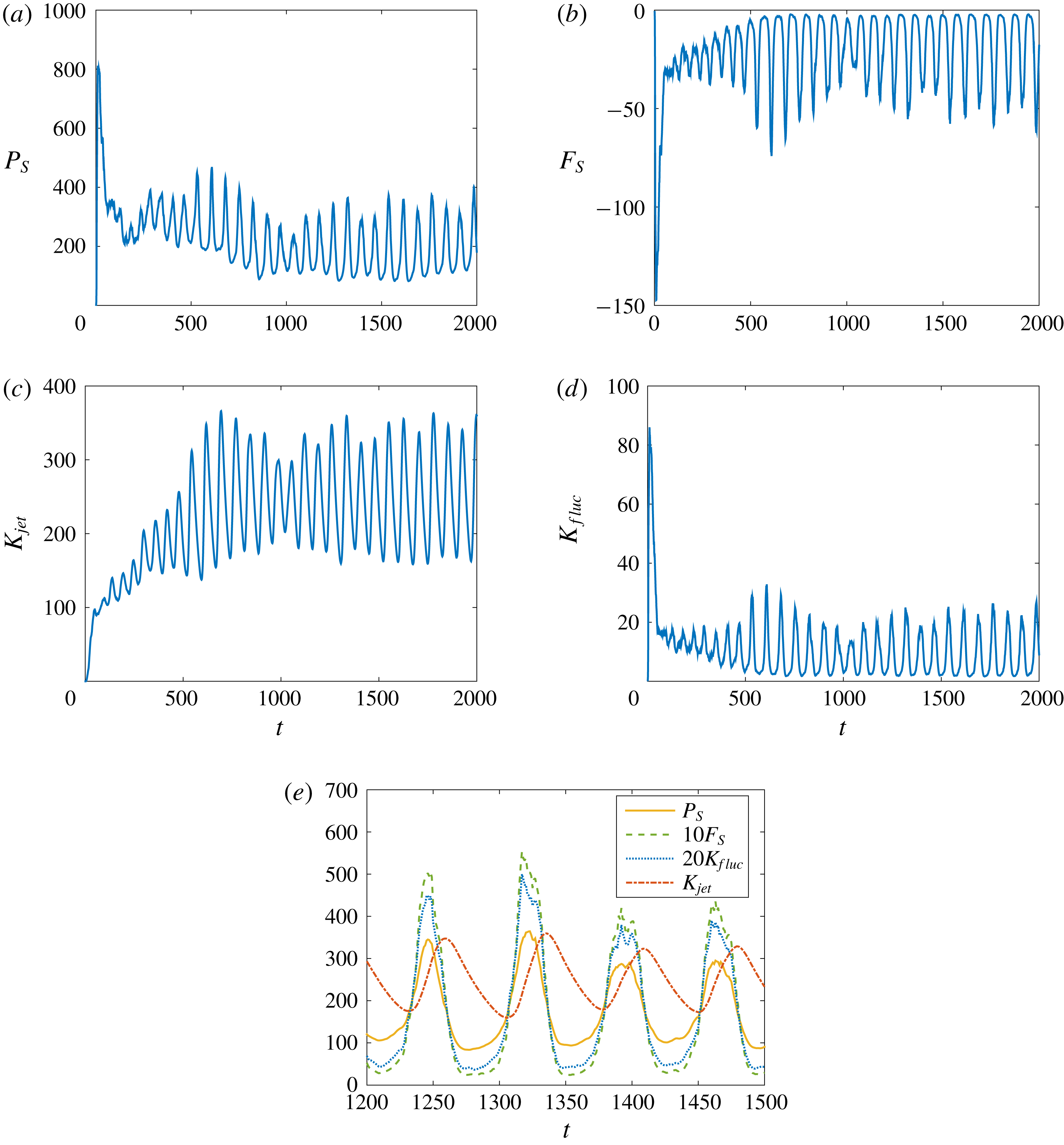
In this parameter regime the MRBC system exhibits remarkable relaxation oscillations that are also shared by the primitive equations (Garaud & Brummell Reference Garaud and Brummell2015). After an initial transient, a statistically stationary state is achieved in which the four global quantities defined in (3.2) all oscillate with a well-defined period but fluctuate in amplitude. Figure 2(e) shows that the salinity potential energy $P_{S}$ , salinity flux $F_{S}$ and the fluctuation kinetic energy $K_{fluc}$ all oscillate in phase but that the kinetic energy $K_{jet}$ in the jets lags behind. The presence of very similar behaviour in both the primitive equations and the asymptotic MRBC system indicates that the latter is not missing any essential physics. We understand this behaviour as follows: efficient fingering, characterized by large salinity flux $F_{S}$ , drives horizontal jets resulting in the growth of $K_{jet}$ . The strengthening jets shear out the salt-finger field (Linden Reference Linden1974; Smyth & Kimura Reference Smyth and Kimura2007; Fernandes & Krishnamurti Reference Fernandes and Krishnamurti2010; Radko Reference Radko2010; Radko et al. Reference Radko, Ball, Colosi and Flanagan2015), resulting in an abrupt collapse of the fluctuations that feed the jets. As a result the jet starts to weaken, and when it is weak enough the fluctuations driven by the salinity stratification regrow and the jet starts to strengthen again. This process then repeats, leading to the observed relaxation oscillations (Garaud & Brummell Reference Garaud and Brummell2015). A similar mechanism is responsible for relaxation oscillations in two-dimensional high- $\mathit{Ra}$ , moderate- $\mathit{Pr}$ Rayleigh–Bénard convection (Rucklidge & Matthews Reference Rucklidge and Matthews1996; Fitzgerald & Farrell Reference Fitzgerald and Farrell2014; Goluskin et al. Reference Goluskin, Johnston, Flierl and Spiegel2014), in three-dimensional Rayleigh–Bénard convection (Matthews et al. Reference Matthews, Rucklidge, Weiss and Proctor1996) and in magnetoconvection (Rucklidge & Matthews Reference Rucklidge and Matthews1996). In § 6 we use this idea to propose a phenomenological model of these relaxation oscillations in order to explain the observed $\mathit{Ra}$ -dependence of the jet properties.

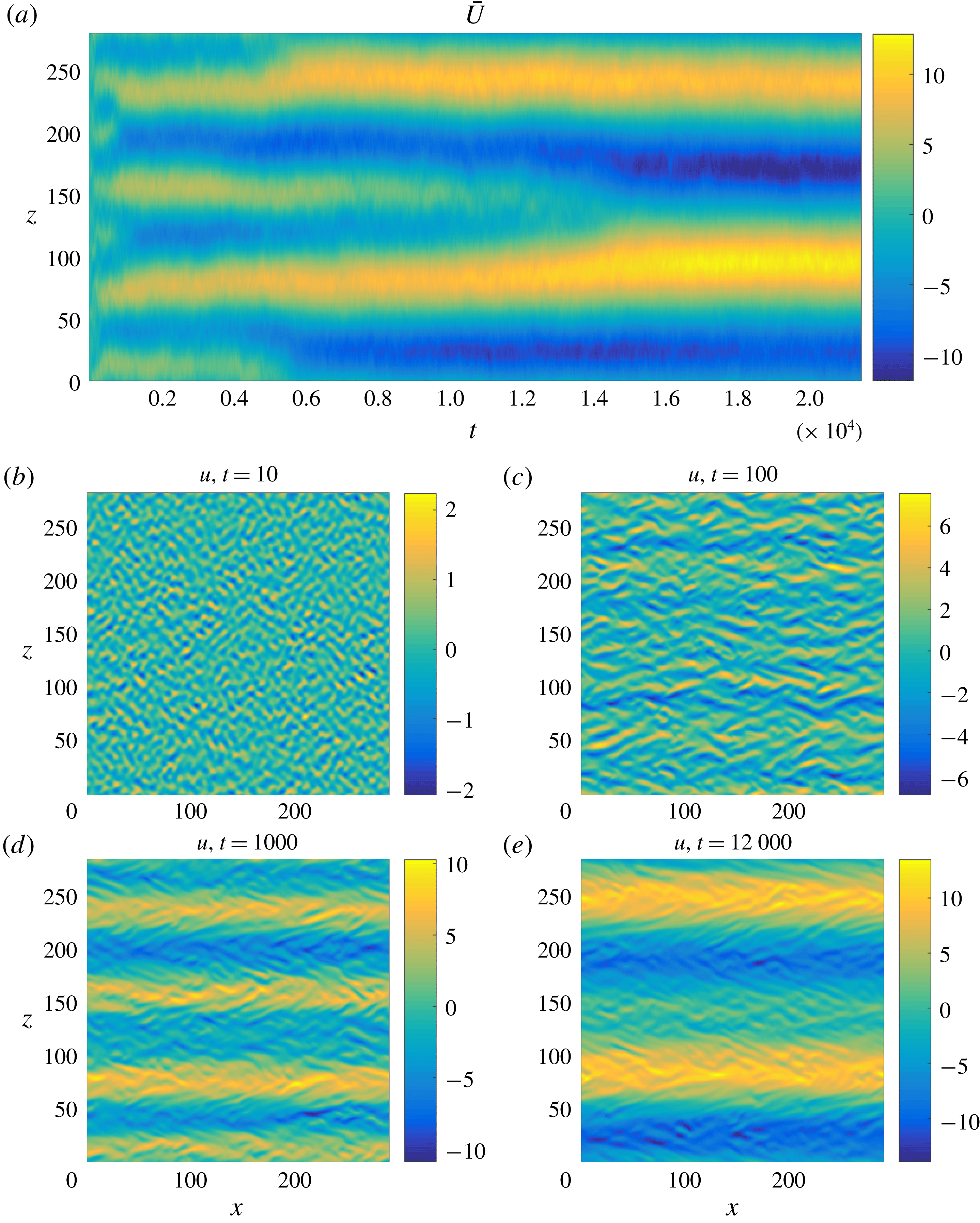
The evolution of the jets in time is shown in figure 3 in terms of a space–time Hovmöller plot of the horizontally averaged horizontal velocity $\bar{U}(z,t)$ . The jets initially coarsen, but subsequently the coarsening process appears to terminate. Superposed on the jets are relaxation oscillations that are observed at all times after an initial transient. These oscillations are almost exactly in phase in all the jets, even though the jets are not all equally strong.

Figure 3.

Space–time evolution of the jet profile $\bar{U}(z,t)$ in the MRBC system when $\mathit{Ra}=6$ and $\mathit{Sc}=1$ .

3.2 Simulation of the MRBC system with $\mathit{Ra}=2$ , $\mathit{Sc}=1$

In this section we show the corresponding results with $\mathit{Ra}=2$ and $\mathit{Sc}=1$ in a doubly periodic domain of the same effective size $L_{x}\times L_{z}=32l_{opt}\times 32l_{opt}$ , with $l_{opt}$ now computed for $\mathit{Ra}=2$ . In this case the density ratio is three times larger and comparable to the inverse of the small diffusivity ratio. This parameter regime is hard to reach in DNS of the primitive equations describing salt-finger convection owing to the high buoyancy frequency associated with large density ratios (Garaud & Brummell Reference Garaud and Brummell2015). However, the MRBC system (2.1) is quite capable of reaching this extreme parameter regime and at low cost.

In figure 4 we show the time evolution of the salinity potential energy $P_{S}$ , salinity flux $F_{S}$ , kinetic energy $K_{jet}$ in the jets and the fluctuation kinetic energy $K_{fluc}$ . We see that $P_{S}$ , $F_{S}$ and $K_{fluc}$ equilibrate relatively quickly while the jet kinetic energy $K_{jet}$ undergoes several step-like increases that correlate well with jet mergers (figure 5 a). The resulting two-jet state persists for a long time, but not forever: if the calculation is continued to ${\gtrsim}10^{5}$ (not shown) one finds that the two jets eventually also merge and the final state of the system therefore consists of a single jet to the right (accompanied, of course, by a similar jet to the left). Moreover, the relaxation oscillations that proved so dominant at $\mathit{Ra}=6$ are now largely submerged in the fluctuation field.

Figure 4.

Evolution of salinity potential energy $P_{S}$ , salinity flux $F_{S}$ , kinetic energy $K_{jet}$ in the jets and the fluctuation kinetic energy $K_{fluc}$ in a doubly periodic domain of size $L_{x}\times L_{z}=32l_{opt}\times 32l_{opt}$ obtained from the MRBC equations (2.1) when $\mathit{Ra}=2$ and $\mathit{Sc}=1$ . A statistically stationary state is present for $t\gtrsim 1.5\times 10^{4}$ .

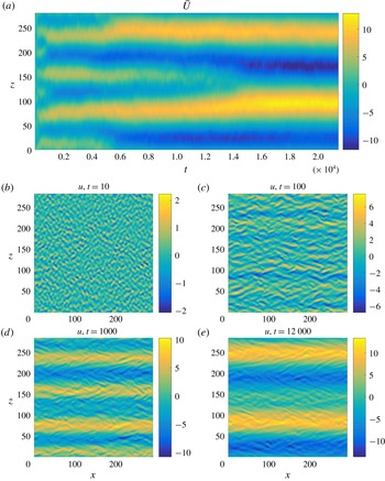
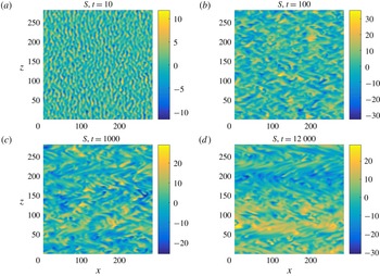
Because of the longer time integration, $t=[0,\,2.2\times 10^{4}]$ , as compared with that in § 3.1, we observe more coarsening events – the four jets coarsen into three around $t=5000$ and then into two around $t=14\,000$ . The snapshots of the horizontal velocity field $u(x,z,t)$ (figure 5 b–e) show that at the very initial time, the salt-finger distribution is almost uniform in height, with no hint of jet formation. However, as time proceeds, jets begin to form and strengthen as a result of repeated mergers. Figure 6 shows the corresponding snapshots of the salinity field $S$ . The salt fingers are clearly visible in the initial stages of evolution but are subsequently shredded by the growing horizontal flow.

Figure 5.

(a) Space–time evolution of the jet profile $\bar{U}(z,t)$ in the MRBC system when $\mathit{Ra}=2$ and $\mathit{Sc}=1$ . (b–e) Snapshots of $u(x,z,t)$ at $t=10,\,100,\,1000$ and $12\,000$ , respectively.

Figure 6.

(a–d) Snapshots of $S(x,z,t)$ at $t=10,\,100,\,1000$ and $12\,000$ , respectively.

To describe the jets we define the dominant jet wavenumber

(3.3) $$\begin{eqnarray}m_{\mathit{dominant}}=\frac{\displaystyle \int |m|^{3}|\hat{\bar{\unicode[STIX]{x1D713}}}|^{2}\,\text{d}m}{\displaystyle \int |m|^{2}|\hat{\bar{\unicode[STIX]{x1D713}}}|^{2}\,\text{d}m},\end{eqnarray}$$

where $\hat{\bar{\unicode[STIX]{x1D713}}}$ is the Fourier transform of the horizontally averaged streamfunction $\bar{\unicode[STIX]{x1D713}}$ . Figure 7 shows the dependence of the total kinetic energy on the dominant jet wavenumber during a simulation run, with the latter normalized by the wavenumber corresponding to the domain height. Thus, at the end of this simulation, $2\unicode[STIX]{x03C0}m/L_{z}$ reaches $2$ . We observe that as the system evolves, the dominant wavenumber decreases and the jet kinetic energy surpasses the fluctuation kinetic energy. In addition, we identify a scaling law for the total kinetic energy, $K_{tot}\sim m_{\mathit{dominant}}^{-\unicode[STIX]{x1D6FC}}$ with $5/3\lesssim \unicode[STIX]{x1D6FC}\lesssim 2$ , quantifying the growth in kinetic energy as the system coarsens.

Figure 7.

Dependence of the total kinetic energy $K_{tot}$ (blue solid curve), the kinetic energy $K_{jet}$ in the jets (red dashed curve) and the kinetic energy $K_{fluc}$ in the fluctuations (green dotted curve) on the dominant jet wavenumber $m_{\text{dominant}}$ . The black arrow indicates the direction of time evolution. The black dashed and dot-dashed lines represent $m^{-2}$ and $m^{-5/3}$ relations, respectively, and are provided for visual guidance.

To illuminate the details of this energy increase, we show in figure 8 the spectrum of the jet kinetic energy

(3.4) $$\begin{eqnarray}E_{Kjet}={\textstyle \frac{1}{2}}m^{2}|\hat{\unicode[STIX]{x1D713}}(0,m)|^{2}\end{eqnarray}$$

at $t=3000$ , $8000$ and $15\,000$ , corresponding to states with $4$ , $3$ and $2$ jets, respectively (figure 5 a). We observe that except on the largest scales, the jet kinetic energy spectrum exhibits a $m^{-4}$ scaling, for which we provide an explanation in § 5. We can also identify a bulge in energy at the largest scale present and track it to yet larger scales as time progresses and the system coarsens. Throughout the paper, we use the notation $E$ to denote spectra – for example, if $K_{jet}$ is the domain-averaged jet kinetic energy then $E_{Kjet}$ is the corresponding spectrum.

Figure 8.

Jet kinetic energy spectrum at $t=3000$ , $8000$ and $15\,000$ . The black dot-dashed line represents the $m^{-4}$ relation and is provided for visual guidance.

We next focus on gathering information about the dynamics and dominant balances in the MRBC system (2.1) in spectral space. For this purpose we observe that in spectral space

(3.5) $$\begin{eqnarray}\frac{\text{d}}{\text{d}t}E_{Ktot}=T_{\unicode[STIX]{x1D713}}+F_{\unicode[STIX]{x1D713}}-Dl_{\unicode[STIX]{x1D713}}-Ds_{\unicode[STIX]{x1D713}},\end{eqnarray}$$

where

(3.6a ) $$\begin{eqnarray}\displaystyle E_{Ktot} & = & \displaystyle {\textstyle \frac{1}{2}}(k^{2}+m^{2})|\hat{\unicode[STIX]{x1D713}}(k,m)|^{2},\end{eqnarray}$$

(3.6b ) $$\begin{eqnarray}\displaystyle T_{\unicode[STIX]{x1D713}} & = & \displaystyle {\textstyle \frac{1}{2}}(\hat{\unicode[STIX]{x1D713}}^{\ast }\widehat{{\mathcal{J}}(\unicode[STIX]{x1D713},\unicode[STIX]{x1D6FB}^{2}\unicode[STIX]{x1D713})}+\text{c.c.}),\end{eqnarray}$$

(3.6c ) $$\begin{eqnarray}\displaystyle F_{\unicode[STIX]{x1D713}} & = & \displaystyle -{\textstyle \frac{1}{2}}(\text{i}k\hat{\unicode[STIX]{x1D713}}{\hat{S}}^{\ast }+\text{c.c.}),\end{eqnarray}$$

(3.6d ) $$\begin{eqnarray}\displaystyle Dl_{\unicode[STIX]{x1D713}} & = & \displaystyle \frac{k^{2}}{k^{2}+m^{2}}|\hat{\unicode[STIX]{x1D713}}(k,m)|^{2},\end{eqnarray}$$

(3.6e ) $$\begin{eqnarray}\displaystyle Ds_{\unicode[STIX]{x1D713}} & = & \displaystyle (k^{2}+m^{2})^{2}|\hat{\unicode[STIX]{x1D713}}(k,m)|^{2}.\end{eqnarray}$$

Here the superscript * indicates a complex conjugate. Equation (3.5) describes the contributions to the evolution of $E_{Ktot}$ arising from energy transport through advection ( $T_{\unicode[STIX]{x1D713}}$ ) and buoyancy ( $F_{\unicode[STIX]{x1D713}}$ ) together with energy losses via large-scale ( $Dl_{\unicode[STIX]{x1D713}}$ ) and small-scale ( $Ds_{\unicode[STIX]{x1D713}}$ ) dissipation. Next, we introduce a decomposition into a mean and a fluctuating part, $\unicode[STIX]{x1D713}=\bar{\unicode[STIX]{x1D713}}+\unicode[STIX]{x1D713}^{\prime }$ , and separate the fluctuation transport equation into mean–fluctuation and fluctuation–fluctuation contributions, defined as follows:

(3.7a ) $$\begin{eqnarray}\displaystyle T_{\unicode[STIX]{x1D713},m+f\rightarrow f} & = & \displaystyle {\textstyle \frac{1}{2}}(\hat{\unicode[STIX]{x1D713}}^{\prime \ast }\widehat{(\unicode[STIX]{x1D713}_{x}^{\prime }\bar{\unicode[STIX]{x1D713}}_{zzz}-\bar{\unicode[STIX]{x1D713}}_{z}\unicode[STIX]{x1D6FB}^{2}\unicode[STIX]{x1D713}_{x}^{\prime })}+\text{c.c.}),\end{eqnarray}$$

(3.7b ) $$\begin{eqnarray}\displaystyle T_{\unicode[STIX]{x1D713},f+f\rightarrow f} & = & \displaystyle {\textstyle \frac{1}{2}}(\hat{\unicode[STIX]{x1D713}}^{\prime \ast }\widehat{{\mathcal{J}}(\unicode[STIX]{x1D713}^{\prime },\unicode[STIX]{x1D6FB}^{2}\unicode[STIX]{x1D713}^{\prime })}+\text{c.c.}).\end{eqnarray}$$

Thus $T_{\unicode[STIX]{x1D713},f}=T_{\unicode[STIX]{x1D713},m+f\rightarrow f}+T_{\unicode[STIX]{x1D713},f+f\rightarrow f}$ is the total fluctuation transport.

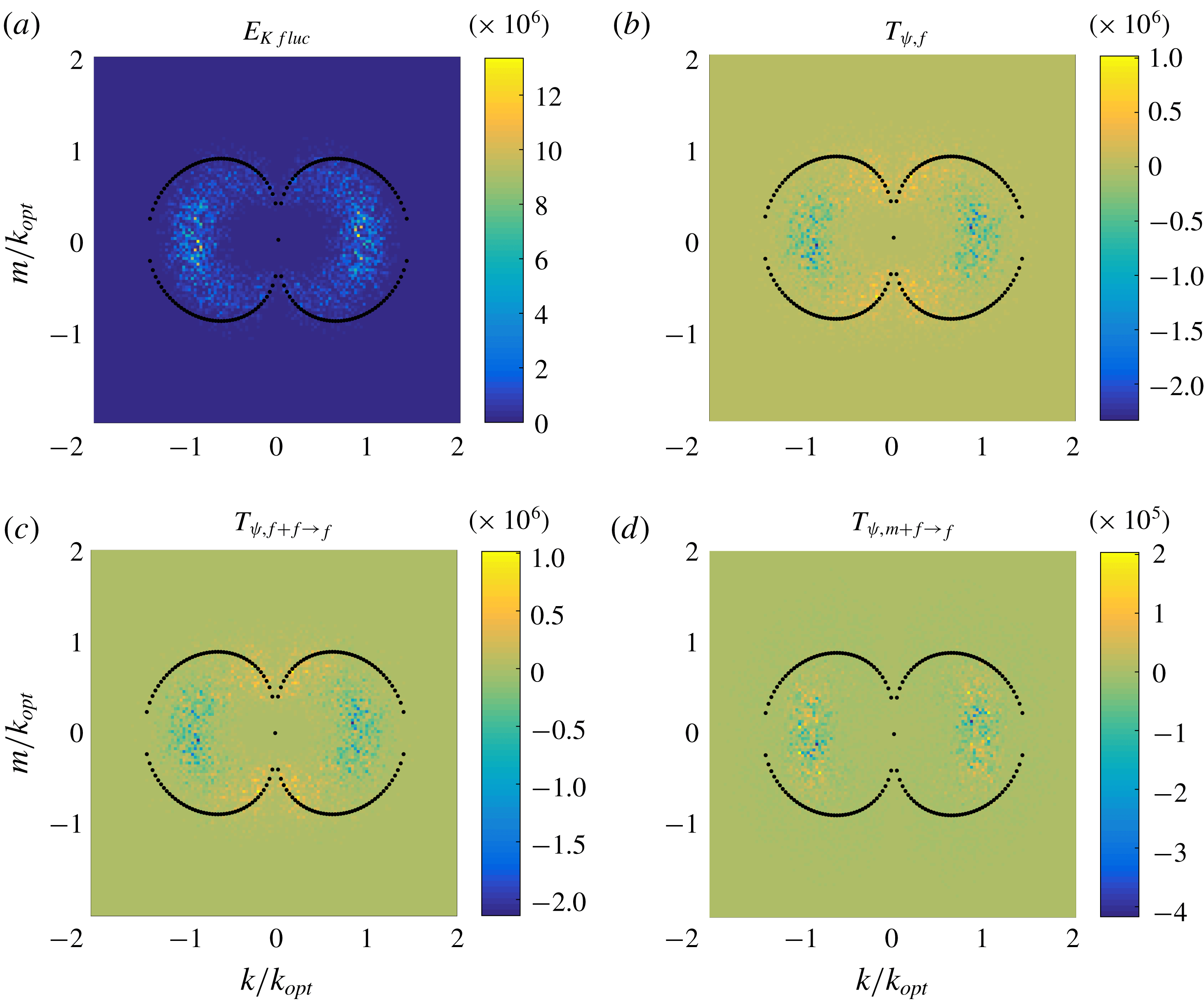
We begin by focusing on the fluctuating component by subtracting the spectrum of the mean from the total spectrum, and define the fluctuation kinetic energy spectrum as $E_{Kfluc}=E_{Ktot}-E_{Kjet}$ . In figure 9 we show the fluctuation spectrum $E_{Kfluc}$ at $t=10$ , the initial stage of evolution. Figure 9(a) shows that the fluctuation kinetic energy initially centres on the optimal wavenumber for instability, much as in the IFSC regime in the limit $\mathit{Sc}\rightarrow \infty$ . Comparison of panels (b–d) shows that advection is dominated by the fluctuation–fluctuation interaction, while the mean–fluctuation interaction is of higher order, as is made explicit by the colour difference in the associated colour maps. The transport of energy from small scales to large scales (inverse cascade) via the fluctuation–fluctuation interaction resembles that in 2D turbulence. This is illustrated in figure 9(c) by the extraction and injection of energy around the optimal wavenumber and marginal curve at $k=0$ , respectively.

Figure 9.

Spectra of (a) the fluctuation kinetic energy $E_{Kfluc}$ , (b) energy transport $T_{\unicode[STIX]{x1D713},f}$ , (c) fluctuation–fluctuation interaction $T_{\unicode[STIX]{x1D713},f+f\rightarrow f}$ and (d) the mean–fluctuation interaction $T_{\unicode[STIX]{x1D713},m+f\rightarrow f}$ at $t=10$ , computed from the MRBC system (2.1) with $\mathit{Ra}=2$ and $\mathit{Sc}=1$ . The black dots mark the marginal curve for linear instability.

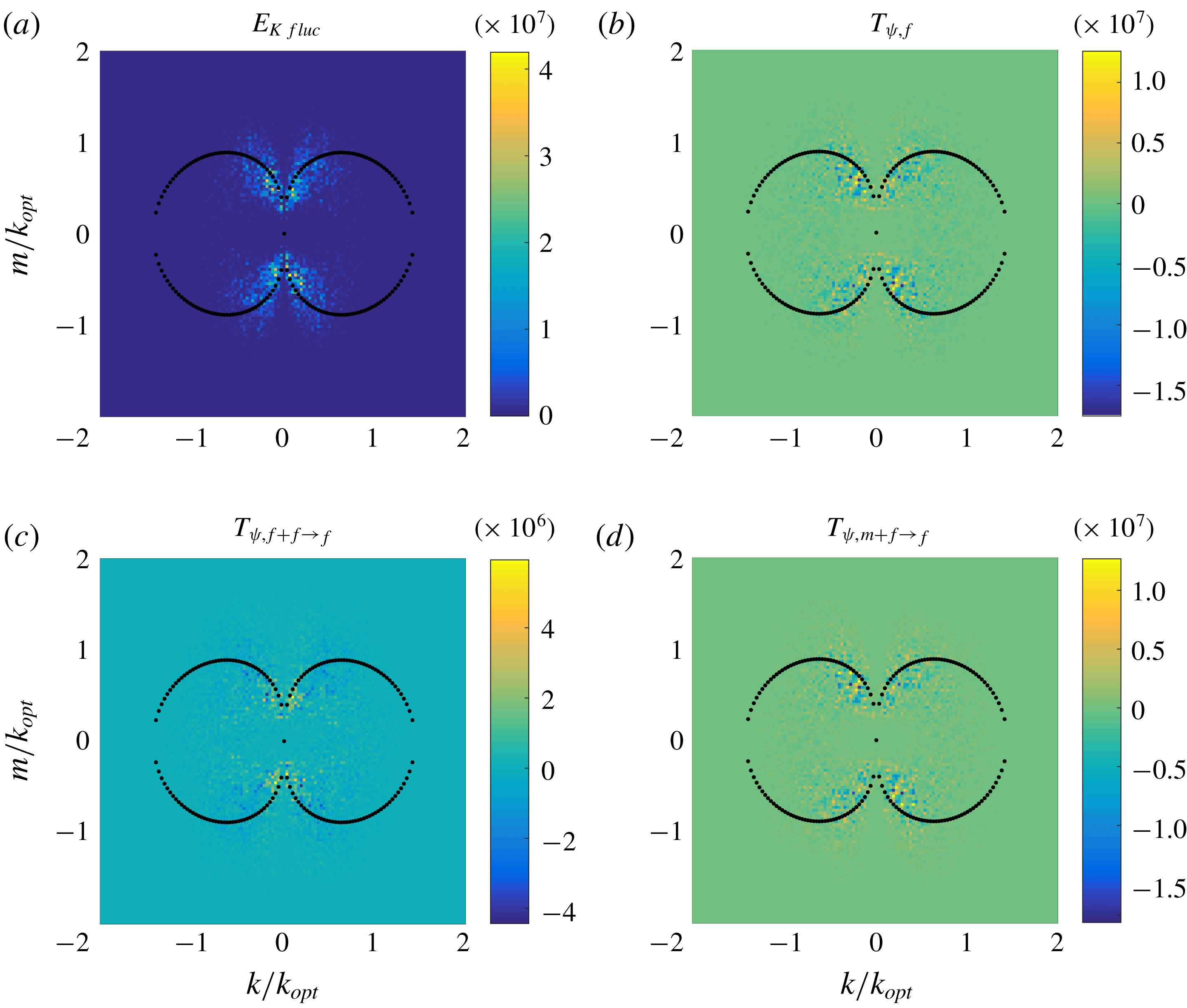
When jets form, the dominant balance changes. In figure 10 we show the spectra of the various contributions to (3.5) at $t=1000$ . The fluctuation kinetic energy spectrum no longer concentrates around the optimal wavenumber, but now centres around the marginal curve at $k\approx 0$ . In addition, as evidenced by the differing range of scale in the colour maps, the dominant component in energy transport is now the mean–fluctuation interaction instead of the fluctuation–fluctuation interaction. We will make use of this important observation in the next section.

Figure 10.

Spectra of (a) the fluctuation kinetic energy $E_{Kfluc}$ , (b) energy transport $T_{\unicode[STIX]{x1D713},f}$ , (c) fluctuation–fluctuation interaction $T_{\unicode[STIX]{x1D713},f+f\rightarrow f}$ and (d) the mean–fluctuation interaction $T_{\unicode[STIX]{x1D713},m+f\rightarrow f}$ at $t=1000$ , computed from the MRBC system (2.1) with $\mathit{Ra}=2$ and $\mathit{Sc}=1$ . The black dots mark the marginal curve for linear instability.

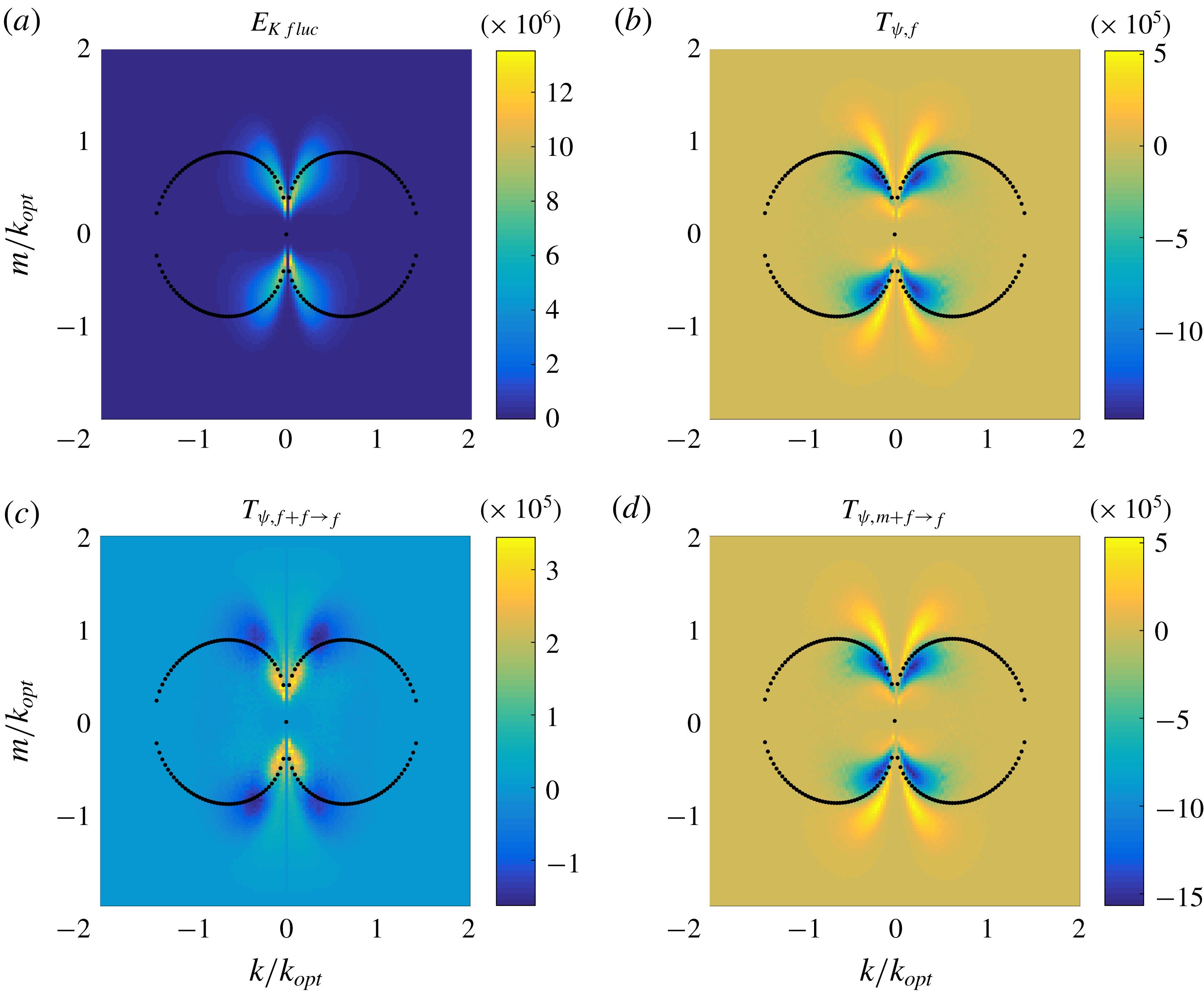
The direction of transport is revealed in figure 11, which shows the spectra of the various contributions to (3.5) averaged over $t=[9000,\,12\,000]$ , a time interval corresponding to the presence of three jets. The fluctuation kinetic energy spectrum $E_{Kfluc}$ centres around the marginal curve and transport is dominated by the mean–fluctuation interactions. The latter transport energy from small to large scales along the marginal curve, while the mean–fluctuation interaction transports energy mostly across the marginal curve.

Figure 11.

Spectra of (a) the fluctuation kinetic energy $E_{Kfluc}$ , (b) the energy transport $T_{\unicode[STIX]{x1D713},f}\equiv T_{\unicode[STIX]{x1D713},f+f\rightarrow f}+T_{\unicode[STIX]{x1D713},m+f\rightarrow f}$ , and its decomposition into (c) the fluctuation–fluctuation interaction $T_{\unicode[STIX]{x1D713},f+f\rightarrow f}$ and (d) the mean–fluctuation interaction $T_{\unicode[STIX]{x1D713},m+f\rightarrow f}$ averaged over $t=[9000,\,12\,000]$ , as computed from the MRBC system (2.1) with $\mathit{Ra}=2$ and $\mathit{Sc}=1$ . The black dots mark the marginal curve for linear instability.

We can obtain an analogous description of salinity transport in spectral space. Multiplying (2.1a ) by ${\hat{S}}^{\ast }$ and adding the complex conjugate leads to the potential energy equation

(3.8) $$\begin{eqnarray}\frac{\text{d}}{\text{d}t}E_{S}=T_{S}+F_{S}-D_{S},\end{eqnarray}$$

where

(3.9a ) $$\begin{eqnarray}\displaystyle E_{S} & = & \displaystyle {\textstyle \frac{1}{2}}|{\hat{S}}(k,m)|^{2},\end{eqnarray}$$

(3.9b ) $$\begin{eqnarray}\displaystyle T_{S} & = & \displaystyle {\textstyle \frac{1}{2}}(\hat{\unicode[STIX]{x1D713}}^{\ast }\widehat{{\mathcal{J}}(\unicode[STIX]{x1D713},S)}+\text{c.c.}),\end{eqnarray}$$

(3.9c ) $$\begin{eqnarray}\displaystyle F_{S} & = & \displaystyle +{\textstyle \frac{1}{2}}(\text{i}k\hat{\unicode[STIX]{x1D713}}{\hat{S}}^{\ast }+\text{c.c.})=-F_{\unicode[STIX]{x1D713}},\end{eqnarray}$$

(3.9d ) $$\begin{eqnarray}\displaystyle D_{S} & = & \displaystyle (k^{2}+m^{2})|{\hat{S}}(k,m)|^{2}.\end{eqnarray}$$

As before, we define the jet and fluctuation parts of the salinity potential energy spectrum

(3.10a ) $$\begin{eqnarray}\displaystyle E_{Sjet} & = & \displaystyle {\textstyle \frac{1}{2}}|{\hat{S}}(0,m)|^{2},\end{eqnarray}$$

(3.10b ) $$\begin{eqnarray}\displaystyle E_{Sfluc} & = & \displaystyle E_{S}-E_{Sjet},\end{eqnarray}$$

and the mean–fluctuation and fluctuation–fluctuation transports:

(3.11a ) $$\begin{eqnarray}\displaystyle T_{S,m+f\rightarrow f} & = & \displaystyle {\textstyle \frac{1}{2}}(S^{\prime \ast }\widehat{(\unicode[STIX]{x1D713}_{x}^{\prime }\bar{S}_{z}-S_{x}^{\prime }\bar{\unicode[STIX]{x1D713}}_{z})}+\text{c.c.}),\end{eqnarray}$$

(3.11b ) $$\begin{eqnarray}\displaystyle T_{S,f+f\rightarrow f} & = & \displaystyle {\textstyle \frac{1}{2}}(S^{\prime \ast }\widehat{{\mathcal{J}}(\unicode[STIX]{x1D713}^{\prime },S^{\prime })}+\text{c.c.}),\end{eqnarray}$$

(3.11c ) $$\begin{eqnarray}\displaystyle T_{S,f} & = & \displaystyle T_{S,m+f\rightarrow f}+T_{S,f+f\rightarrow f}.\end{eqnarray}$$

Figure 12 shows $E_{Sfluc}$ and $T_{S,f}$ averaged over $t=[9000,\,12\,000]$ . The salinity field differs from the streamfunction by its concentration at large scale both horizontally and vertically.

Figure 12.

Spectra of (a) the fluctuation salinity potential energy $E_{Sfluc}$ , (b) the salinity transport $T_{S,f}\equiv T_{S,f+f\rightarrow f}+T_{S,m+f\rightarrow f}$ and its decomposition into (c) the fluctuation–fluctuation interaction $T_{S,f+f\rightarrow f}$ and (d) the mean–fluctuation interaction $T_{S,m+f\rightarrow f}$ averaged over $t=[9000,\,12\,000]$ , as computed from the MRBC system (2.1) with $\mathit{Ra}=2$ and $\mathit{Sc}=1$ . The black dots mark the marginal curve for linear instability.

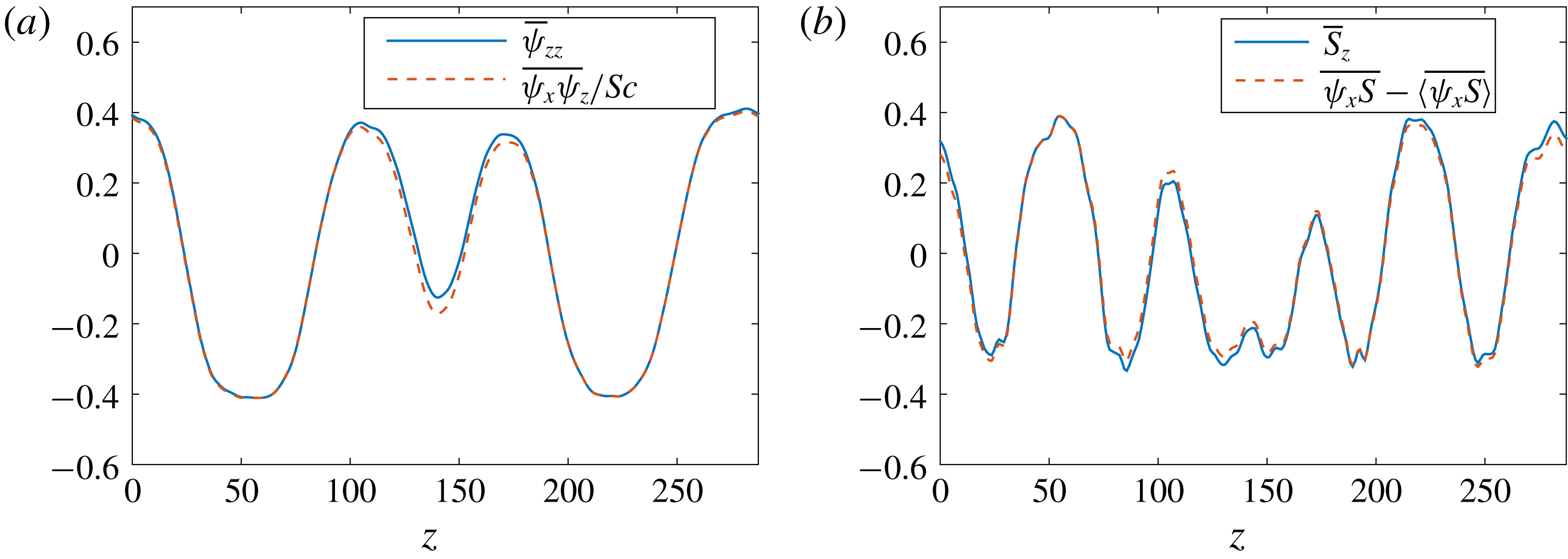
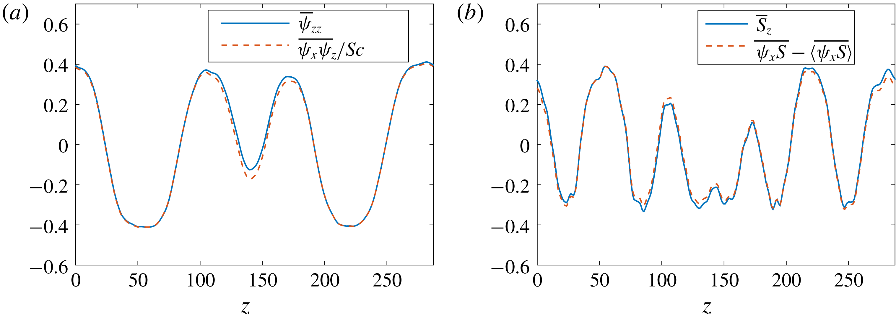
To understand the mean balance, we take the time and horizontal (zonal) average over a statistically steady state of the MRBC system (2.1). We obtain

(3.12a ) $$\begin{eqnarray}\displaystyle \frac{1}{\mathit{Sc}}\overline{\unicode[STIX]{x1D713}_{x}\unicode[STIX]{x1D713}_{z}}=\bar{\unicode[STIX]{x1D713}}_{zz}, & & \displaystyle\end{eqnarray}$$

(3.12b ) $$\begin{eqnarray}\displaystyle \overline{\unicode[STIX]{x1D713}_{x}S}=\bar{S}_{z}+\text{const.}, & & \displaystyle\end{eqnarray}$$

a result confirmed in figure 13, indicating that the system has reached a statistically steady state in which the jet structure is in balance with dissipation. In (3.12b ) the constant of integration corresponds to the total downward salinity flux that drives the system by transferring available potential energy in the salinity field into kinetic energy, and hence must be non-zero. In contrast, equation (3.12a ) contains no integration constant because the $x\rightarrow -x$ symmetry of the MRBC model prohibits shear with a preferred direction. The small differences between the left- and right-hand sides of (3.12) seen in figure 13 are a consequence of the slow coarsening process.

Figure 13.

Contributions to the balance equations (3.12) for the MRBC system (2.1) with $\mathit{Ra}=2$ and $\mathit{Sc}=1$ , time-averaged over $t=[9000,\,12\,000]$ . (a) Mean $\unicode[STIX]{x1D713}$ balance. (b) Mean $S$ balance.

4 Further reduction

In the previous section we found that horizontal jets are the dominant structures in the MRBC system (2.1) at late times and that in the jet regime the mean–fluctuation interaction is stronger than the fluctuation–fluctuation interaction. In this section we make use of these findings to obtain two further simplifications of the MRBC system that continue to retain the essential dynamics of this system. These are the quasilinear system studied in § 4.1, obtained by neglecting the fluctuation–fluctuation interaction, and the single-mode system studied in § 4.2, with only one horizontal wavenumber. The results show that these two further reductions do, at least qualitatively, capture the phenomena of jet formation and coarsening, and provide us with additional confidence in the phenomenological theory described in § 5.

4.1 Quasilinear system

In this section, we present the study of the quasilinear system obtained by neglecting the fluctuation–fluctuation interaction in the MRBC system (2.1). Mathematically, we replace the nonlinear advection terms by their quasilinear approximation:

(4.1) $$\begin{eqnarray}{\mathcal{J}}(a,b)\rightarrow {\mathcal{J}}(\bar{a},b^{\prime })+{\mathcal{J}}(a^{\prime },\bar{b}),\end{eqnarray}$$

where $a$ and $b$ are arbitrary fields. Thus the mean–perturbation interaction contains both the mean-advected perturbation field and the perturbation-advected mean field. This approximation has been widely used in studies of jet formation on the $\unicode[STIX]{x1D6FD}$ -plane with random forcing (cf. Farrell & Ioannou Reference Farrell and Ioannou2003, Reference Farrell and Ioannou2007; O’Gorman & Schneider Reference O’Gorman and Schneider2007; Marston, Conover & Schneider Reference Marston, Conover and Schneider2008; Srinivasan & Young Reference Srinivasan and Young2012) because it leads to a relatively simple description of the statistical properties of the solution in terms of cumulants. However, the quasilinear approximation may apply to deterministic systems as well. In some cases the approximation may be justified by appropriate asymptotic analysis (Beaume et al. Reference Beaume, Chini, Julien and Knobloch2015), but here it is made on the basis of our numerical observations. We show below that the mean–fluctuation interaction alone can generate and maintain horizontal jets, without the presence of an inverse cascade mechanism due to the fluctuation–fluctuation interaction. For this study we therefore retain the parameters $\mathit{Ra}=2$ and $\mathit{Sc}=1$ and likewise retain the domain size and resolution of the previous section, unless otherwise specified.

Figure 14.

Blue solid curves: evolution of the salinity potential energy $P_{S}$ , salinity flux $F_{S}$ , the jet kinetic energy $K_{jet}$ and the kinetic energy $K_{fluc}$ of the associated fluctuations computed from the quasilinear system with $\mathit{Ra}=2$ and $\mathit{Sc}=1$ in a doubly periodic domain of size $L_{x}\times L_{z}=32l_{opt}\times 32l_{opt}$ . Red dashed curves: corresponding quantities from the MRBC system (shown in figure 4).

Figure 15.

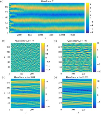
(a) Space–time evolution of the jet profile $\bar{U}(z,t)$ in the quasilinear system when $\mathit{Ra}=2$ and $\mathit{Sc}=1$ . (b–e) Snapshots of $u(x,z,t)$ at $t=10,\,100,\,1000$ and $12\,000$ , respectively.

Numerical integration of the resulting quasilinear system shows that all quantities settle into a statistically steady state, although here they do so much faster than the corresponding quantities in figure 4. In figure 14 we compare the time evolution of the salinity potential energy $P_{S}$ , salinity flux $F_{S}$ , and the kinetic energy $K_{jet}$ and $K_{fluc}$ of the jets and the associated fluctuations in the quasilinear system (blue curves) with the corresponding results from the MRBC model (red curves). The figure shows that the salinity potential energy and the fluctuation kinetic energy in the saturated state are larger than those in the MRBC system, while the salinity flux and the jet kinetic energy are weaker. However, a more careful look reveals that the jet kinetic energy in the quasilinear linear system saturates at approximately the same level as the initial saturation level in the MRBC system, although subsequent coarsening in the latter leads to growing divergence between the two. At the same time the coarsening in the MRBC system leads to growing convergence with the salinity potential energy in the quasilinear system. Figure 15 shows a typical evolution of the horizontally averaged horizontal velocity as well as snapshots of the instantaneous horizontal velocity $u(x,z,t)$ . The key feature we observe is that jets still form, indicating that the primary mechanism behind jet formation is the mean–fluctuation interaction. As in the full system, we observe that initially narrow jets gradually coarsen into fewer broader and more energetic jets, although here the three-jet state appears to be more stable and persists for a longer time than in the MRBC system. However, the structure of the fluctuating horizontal velocity field $u(x,z,t)$ differs in detail from that of the MRBC system (figure 5), with small horizontal scale structures suppressed and replaced over time by prominent V-shaped structures that stretch across the domain in the horizontal direction (figure 15 b–e).

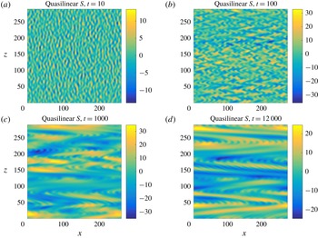
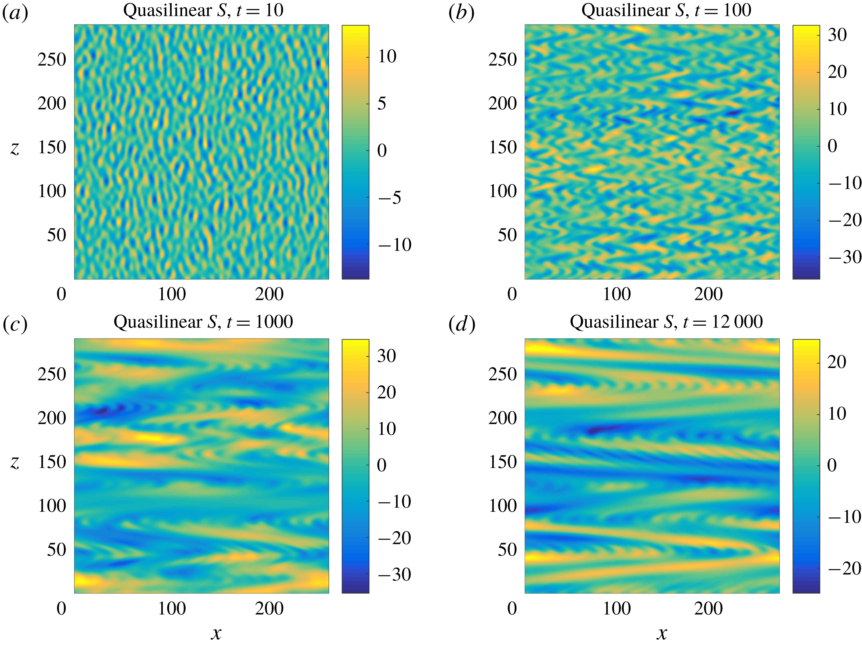
Figure 16 shows the corresponding snapshots of the salinity field $S(x,z,t)$ , whose behaviour also resembles that of the full MRBC system (figure 6) – as the mean velocity field strengthens with time, it shears the salt fingers more efficiently and we observe smaller-scale fingers. These are gradually submerged into horizontal domain-size structures reflecting similar structures in the $u(x,z,t)$ snapshots. Qualitatively similar results were obtained for moderately low Prandtl numbers by Radko (Reference Radko2010) using a weakly nonlinear mean-field approach.

Figure 16.

(a–d) Snapshots of $S(x,z,t)$ at $t=10,\,100,\,1000$ and $12\,000$ , respectively, for the quasilinear system with $\mathit{Ra}=2$ , $\mathit{Sc}=1$ .

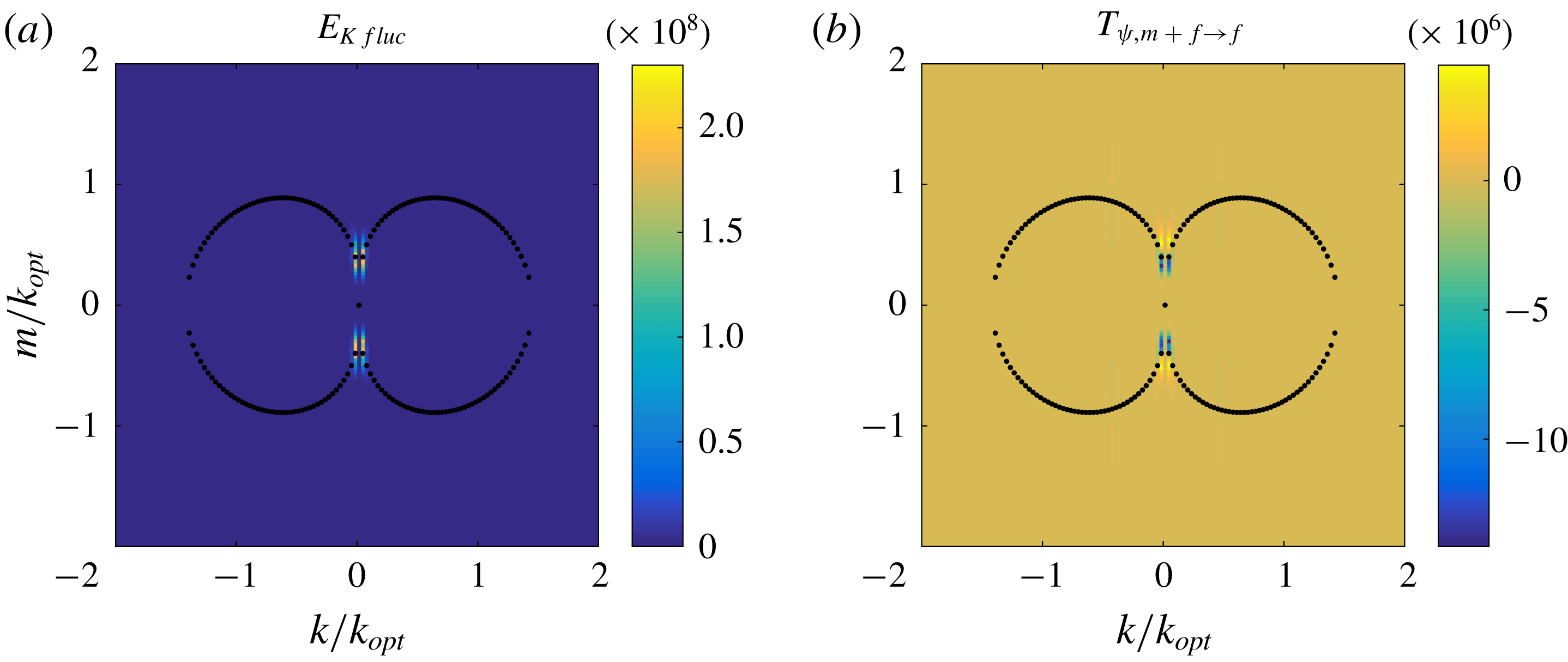
We conclude this subsection with figure 17, showing the spectrum of the fluctuation kinetic energy $E_{Kfluc}$ and the transport term $T_{\unicode[STIX]{x1D713}}$ averaged over $t=[10\,000,\,11\,000]$ . The figure shows that the fluctuation kinetic energy concentrates at the horizontal wavenumber corresponding to the domain size while centring around the marginal curve. These large horizontal scale structures are particularly prominent in figure 15(e). From the transport term shown in figure 17(b) we see that advection transports energy from linearly growing modes to linearly damped modes, much as occurs in the full MRBC system.

Figure 17.

(a,b) Spectra of the fluctuation kinetic energy $E_{Kfluc}$ and energy transport $T_{\unicode[STIX]{x1D713},f}$ in the quasilinear system arising from the mean–fluctuation interaction, averaged over $t=[10\,000,\,11\,000]$ . The black dots mark the marginal curve for linear instability.

4.2 Single-mode system

In the previous section we found that the quasilinear system can successfully generate jets and that energy concentrates at the largest horizontal scales accessible to the system. In this section we use this information to reduce the quasilinear system yet further, to a single-mode system with only one horizontal wavenumber corresponding to the domain size, $k=\unicode[STIX]{x03C0}/(16l_{opt})$ , retained in the fluctuation field. As before we present results from this procedure for the parameters $\mathit{Ra}=2$ and $\mathit{Sc}=1$ .

Figure 18 shows the time evolution of the salinity potential energy $P_{S}$ , salinity flux $F_{S}$ , kinetic energy $K_{jet}$ in the jets and the kinetic energy $K_{fluc}$ in the associated fluctuations and compares it with the evolution of the corresponding quantities in the MRBC system. As in the quasilinear system, the single-mode system also shows an initial energy peak, but this time the ‘final’ state is not as steady and bursts appear in the energy evolution. This abrupt bursting behaviour is also observed in the evolution of the jet state shown in figure 19. The main distinguishing feature of the single-mode system is that the jet coarsens to the domain size very quickly, but the subsequent properties of the jet structure are qualitatively similar to those found in both the quasilinear system and the MRBC system. Indeed, figure 18 shows that the salinity potential energy and the fluctuation kinetic energy are reproduced almost perfectly, although the salinity flux and the jet kinetic energy are in general weaker.

Figure 18.

Blue solid curves: evolution of the salinity potential energy $P_{S}$ , salinity flux $F_{S}$ , the jet kinetic energy $K_{jet}$ and the kinetic energy $K_{fluc}$ of the associated fluctuations computed from the single-mode system with $\mathit{Ra}=2$ and $\mathit{Sc}=1$ and wavenumber $k=\unicode[STIX]{x03C0}/(16l_{opt})$ in a doubly periodic domain of size $L_{x}\times L_{z}=32l_{opt}\times 32l_{opt}$ . Red dashed curves: corresponding quantities from the MRBC system (shown in figure 4).

Figure 19.

Space–time evolution of the jet profile $\bar{U}(z,t)$ in the single-mode system with $\mathit{Ra}=2$ and $\mathit{Sc}=1$ and wavenumber $k=\unicode[STIX]{x03C0}/(16l_{opt})$ .

5 Spectra

In the previous section we showed that the quasilinear and single-mode models capture the essential behaviour of the MRBC model – jet formation and coarsening – despite differences in the detailed properties of the solutions. In this section we perform a more quantitative comparison by comparing and contrasting in detail the spectra of the solutions to the MRBC model and the quasilinear and single-mode approximations to it.

Figure 20 shows that all three systems exhibit the same zonal velocity spectrum $\bar{E}_{u}(m)=|\hat{u} (k=0,m)|^{2}/2\sim m^{-4}$ and the same mean salinity spectrum $\bar{E}_{Sjet}(m)=|{\hat{S}}(k=0,m)|^{2}/2\sim m^{-2}$ at sufficiently small $m/k_{opt}$ . In view of our reduction procedure, this robust scaling must be a consequence of the mean–fluctuation interaction and insensitive to the fluctuation–fluctuation interactions. In fact, the fluctuation–fluctuation interactions are important only for wavenumbers $m/k_{opt}\gtrsim 0.7$ . We emphasize that this scaling differs from the $m^{-5}$ scaling for the planetary ( $\unicode[STIX]{x1D6FD}$ -plane) jet based on the Rossby wave dispersion relation (Rhines Reference Rhines1975).

Figure 20.

Compensated spectra of (a) the mean velocity and (b) the mean salinity for the MRBC model, the quasilinear (QL) model and the single-mode model with wavenumber $k=\unicode[STIX]{x03C0}/(16l_{opt})$ .

To understand the origin of these large-scale spectral scalings we examine the dominant balances in the governing equations in spectral space. However, finding these balances in the MRBC and quasilinear models is not simple, owing to the $k$ dependence of the terms. Figures 21 and 22 show the $m$ dependence of $E_{\unicode[STIX]{x1D713}}=|\hat{\unicode[STIX]{x1D713}}|^{2}/2$ and $E_{S}=|{\hat{S}}|^{2}/2$ for fixed horizontal wavenumbers $k=2\unicode[STIX]{x03C0}n_{k}/L_{x}$ , $n_{k}=1,\,2\,\ldots ,$ computed from the MRBC and quasilinear models, respectively. We see that while the spectrum of $E_{\unicode[STIX]{x1D713}}$ does depend on $k$ , the $m$ -dependence of $E_{S}$ is almost independent of $k$ . Note that in these figures the quantities marked ‘averaged’ correspond to averaging over all the horizontal wavenumbers $k$ , and not only over the five smallest wavenumbers shown in the plots.

Figure 21.

The quantities $E_{\unicode[STIX]{x1D713}}$ and $E_{S}$ at differing fixed horizontal wavenumbers $k$ computed from the MRBC system with $\mathit{Ra}=2$ , $\mathit{Sc}=1$ . The black curve shows the spectrum obtained by averaging over $k$ . The red star is the marginal vertical wavenumber corresponding to the smallest horizontal wavenumber $2\unicode[STIX]{x03C0}/L_{x}$ . (a) MRBC, fluctuation $\unicode[STIX]{x1D713}$ spectrum. (b) MRBC, fluctuation $S$ spectrum.

Figure 22.

The quantities $E_{\unicode[STIX]{x1D713}}$ and $E_{S}$ at different fixed horizontal wavenumbers $k$ computed from the quasilinear system with $\mathit{Ra}=2$ , $\mathit{Sc}=1$ . The black curve shows the spectrum obtained by averaging over $k$ . The red star is the marginal vertical wavenumber corresponding to the smallest horizontal wavenumber $2\unicode[STIX]{x03C0}/L_{x}$ . (a) QL, fluctuation $\unicode[STIX]{x1D713}$ spectrum. (b) QL, fluctuation $S$ spectrum.

The situation is simpler in the single-mode case. Figure 23 shows the spectra of the different contributions to the fluctuation momentum and fluctuation salinity balance in spectral space ((3.5) and (3.8)) as computed from the single-mode system in a statistically steady state when $\mathit{Ra}=2$ and $\mathit{Sc}=1$ . We find that in the large-scale regime (small $m$ ) all quantities exhibit power-law behaviour. The dominant balance in the momentum equation is between energy pumping by buoyancy $F_{\unicode[STIX]{x1D713}}$ and large-scale damping $Dl_{\unicode[STIX]{x1D713}}$ ; the slight imbalance between the two quantifies the contribution of the transport term $T_{\unicode[STIX]{x1D713}}$ . In the salinity equation, the flux $F_{S}$ , damping $D_{S}$ and the transport term $T_{S}$ are all comparable and in balance.

Figure 23.

Contributions to (a) fluctuating momentum balance and (b) fluctuating salinity balance, in spectral space, obtained from the single-mode model with $\mathit{Ra}=2$ , $\mathit{Sc}=1$ and wavenumber $k=\unicode[STIX]{x03C0}/(16l_{opt})$ . The star is the marginal vertical wavenumber corresponding to $k=\unicode[STIX]{x03C0}/(16l_{opt})$ .

Figure 24 shows the spectrum of the transport term $T_{\unicode[STIX]{x1D713}}$ in the momentum equation. This term consists of two contributions

(5.1a,b ) $$\begin{eqnarray}T_{\unicode[STIX]{x1D713}1}={\textstyle \frac{1}{2}}(\hat{\unicode[STIX]{x1D713}}^{\ast }\widehat{\bar{\unicode[STIX]{x1D713}}_{z}\unicode[STIX]{x1D6FB}^{2}\unicode[STIX]{x1D713}_{x}^{\prime }}+\text{c.c.})\quad \text{and}\quad T_{\unicode[STIX]{x1D713}2}={\textstyle \frac{1}{2}}(\hat{\unicode[STIX]{x1D713}}^{\ast }\widehat{\unicode[STIX]{x1D713}_{x}^{\prime }\bar{\unicode[STIX]{x1D713}}_{zzz}+\text{c.c.}}).\end{eqnarray}$$

Of these $T_{\unicode[STIX]{x1D713}1}$ is the dominant term, while $T_{\unicode[STIX]{x1D713}2}$ has the opposite sign and therefore reduces (slightly) the overall effectiveness of the first term.

Figure 24.

Transport terms in spectral space computed from the single-mode model with $\mathit{Ra}=2$ , $\mathit{Sc}=1$ and wavenumber $k=\unicode[STIX]{x03C0}/(16l_{opt})$ .

We can express the above leading- and next-order balances in the $\unicode[STIX]{x1D713}$ fluctuation equation as

(5.2a ) $$\begin{eqnarray}\displaystyle F_{\unicode[STIX]{x1D713}} & {\sim} & \displaystyle Dl_{\unicode[STIX]{x1D713}},\end{eqnarray}$$

(5.2b ) $$\begin{eqnarray}\displaystyle T_{\unicode[STIX]{x1D713}1} & {\sim} & \displaystyle Dl_{\unicode[STIX]{x1D713}}+F_{\unicode[STIX]{x1D713}},\end{eqnarray}$$

$T_{\unicode[STIX]{x1D713}}$

$T_{\unicode[STIX]{x1D713}1}$

$Dl_{\unicode[STIX]{x1D713}}+F_{\unicode[STIX]{x1D713}}$

$Dl_{\unicode[STIX]{x1D713}}+F_{\unicode[STIX]{x1D713}}\sim mDl_{\unicode[STIX]{x1D713}}$

$k\leqslant m\ll 1$

$\unicode[STIX]{x0394}\sim m^{-2}$

(5.3a ) $$\begin{eqnarray}\displaystyle {\hat{S}}^{\prime } & {\sim} & \displaystyle \frac{1}{m^{2}}\hat{\unicode[STIX]{x1D713}}^{\prime },\end{eqnarray}$$

(5.3b ) $$\begin{eqnarray}\displaystyle \widehat{\bar{\unicode[STIX]{x1D713}}_{z}\unicode[STIX]{x1D6FB}^{2}\unicode[STIX]{x1D713}_{x}^{\prime }} & {\sim} & \displaystyle m\frac{1}{m^{2}}\hat{\unicode[STIX]{x1D713}}^{\prime }.\end{eqnarray}$$

(5.4a ) $$\begin{eqnarray}\displaystyle \widehat{\unicode[STIX]{x1D713}_{z}^{\prime }\unicode[STIX]{x1D713}_{x}^{\prime }}\sim m^{2}\hat{\bar{\unicode[STIX]{x1D713}}}, & & \displaystyle\end{eqnarray}$$

(5.4b ) $$\begin{eqnarray}\displaystyle \widehat{\unicode[STIX]{x1D713}_{x}^{\prime }S^{\prime }}\sim m\hat{\bar{S}}. & & \displaystyle\end{eqnarray}$$

To solve the closed system (5.3)–(5.4) we must compute the convolution integrals. These do not have a suitable asymptotic expansion valid in our large-scale regime, and we therefore calculate them numerically. For this purpose we assume that all quantities are described by piecewise power laws, i.e.

(5.5) $$\begin{eqnarray}\hat{f}(m)=\left\{\begin{array}{@{}l@{}}|m|^{\unicode[STIX]{x1D6FC}},\quad |m|<m_{0},\quad \\ |m|^{\unicode[STIX]{x1D6FD}},\quad |m|\geqslant m_{0},\quad \end{array}\right.\end{eqnarray}$$

where $m_{0}$ denotes the transition between large and small scales. We also assume that the transition between these two regimes occurs at the marginal wavenumber, $m_{0}=m_{\text{mar}}=(\mathit{Ra}-1)^{1/6}k^{1/3}=(\mathit{Ra}-1)^{1/6}(2\unicode[STIX]{x03C0}/L_{x})^{1/3}$ , as observed in figure 23. In the above expressions, the convergence of the Fourier transform requires that $\unicode[STIX]{x1D6FD}<0$ .

Figure 25.

Numerical (green solid curve) and theoretical estimates of the left-hand side of (5.3b ). The theoretical estimates use different values of the small-scale exponent $\unicode[STIX]{x1D6FD}$ : blue curve for $\unicode[STIX]{x1D6FD}=-10$ and red curve for $\unicode[STIX]{x1D6FD}=-\infty$ .

For convenience, we define a function $C(n_{1},n_{2})$ that approximates the exponent of the convolution of two functions $f_{1}$ and $f_{2}$ with the piecewise power-law spectra defined above in (5.5) and large-scale exponents $\unicode[STIX]{x1D6FC}=n_{1}$ and $\unicode[STIX]{x1D6FC}=n_{2}$ , respectively, i.e. $\widehat{f_{1}f_{2}}\sim m^{C(n_{1},n_{2})}$ for $m<m_{0}$ . Here, we assume that $C(n_{1},n_{2})$ is independent of the small-scale exponents, as confirmed numerically in figure 25, and determine this quantity from a power-law fit to the convolution in the range $k\lesssim m\lesssim m_{0}$ . Thus $C(n_{1},n_{2})$ is determined empirically.

Assuming that the fluctuation and mean fields are well approximated for $k\lesssim m\lesssim m_{0}$ by the power laws

(5.6a-d ) $$\begin{eqnarray}\hat{\unicode[STIX]{x1D713}}^{\prime }\sim m^{a},\quad \hat{\bar{\unicode[STIX]{x1D713}}}\sim m^{b},\quad {\hat{S}}^{\prime }\sim m^{c}\quad \text{and}\quad \hat{\bar{S}}\sim m^{d},\end{eqnarray}$$

and that $k\ll 1$ is fixed, a balance of the exponents in (5.3)–(5.4) implies

(5.7a ) $$\begin{eqnarray}\displaystyle c & = & \displaystyle a-2,\end{eqnarray}$$

(5.7b ) $$\begin{eqnarray}\displaystyle C(b+1,a+2) & = & \displaystyle a-1,\end{eqnarray}$$

(5.7c ) $$\begin{eqnarray}\displaystyle C(a+1,a) & = & \displaystyle b+2,\end{eqnarray}$$

(5.7d ) $$\begin{eqnarray}\displaystyle C(a,c) & = & \displaystyle d+1.\end{eqnarray}$$

$m$

$m_{0}$

$m\gtrsim k$

$C(a,b)$

$a$

$b$

(5.8a-d ) $$\begin{eqnarray}a\approx 2,\quad b\approx -3,\quad c\approx 0,\quad d\approx -1\end{eqnarray}$$

is found to lead to smallest error in (5.7) and matches well the numerical results for the mean velocity and salinity spectra presented in figure 20(a,b). Thus despite its empirical nature the above procedure provides a pathway to understanding the origin of the observed large-scale behaviour of the jet spectrum.

In figure 25 we show the matching between the numerical simulation results and the theoretical prediction for the left-hand side of (5.3b ) and hence (5.7b ). The convolution of functions of the form of (5.5) is well approximated by a power law in the large-scale regime. In addition, since the $\unicode[STIX]{x1D6FD}=-10$ and $\unicode[STIX]{x1D6FD}=-\infty$ cases are indistinguishable at large scales, we conclude that the small-scale exponent is unimportant in the computation of $C$ . This provides a plausible explanation why the three systems – MRBC, quasilinear and single mode – all have the same large-scale spectrum, even though their small-scale spectra are very different.

We close this section by discussing the physical space structure corresponding to the large-scale scaling (5.8), focusing on the mean velocity $\bar{U}$ characterizing the jet structure. In view of the scaling $\hat{\bar{\unicode[STIX]{x1D713}}}\sim m^{-3}$ of the mean streamfunction, the mean velocity scales as $\hat{\bar{U}}\sim m^{-2}$ . The inverse-square dependence of the spectrum of the jet velocity $\bar{U}$ on the wavenumber $m$ is consistent with a zigzag profile: at the jet flank the mean velocity depends linearly on $z$ and the shear is therefore constant, $\bar{U}_{z}=\text{const}.$ , a conclusion that is confirmed in figure 26. Similar linkage between a power-law spectrum and spatial structure also appears in other systems. For example, the Phillips spectrum is based on the assumption that gravity waves have a wedge shape (Phillips Reference Phillips1958).

Figure 26.

Mean velocity $\bar{U}$ and shear $\bar{U}_{z}$ for the full MRBC system at $t=20\,000$ .

6 Turbulent Hopf bifurcation

One striking phenomenon observed in the simulations of the MRBC system (2.1), beyond the appearance of jets, is the turbulent state with superposed, approximately periodic oscillations present when $\mathit{Ra}=6$ . In contrast, when $\mathit{Ra}=2$ these oscillations are absent and the state is statistically steady, albeit turbulent. An intriguing question arises therefore as to the mechanism whereby these oscillations first appear as $\mathit{Ra}$ increases from $\mathit{Ra}=2$ . This section is devoted to this question.

Figure 27 shows the projection of the MRBC dynamics on two quantities characteristic of the large-scale dynamics, the kinetic energy $K_{jet}$ in the jets and the salinity potential energy $P_{S}$ , for four values of the Rayleigh ratio, $\mathit{Ra}=2,\,3,\,4$ and $6$ . We see that when $\mathit{Ra}=2$ the system evolves towards a fixed-point attractor corresponding to a statistically steady state. As $\mathit{Ra}$ increases, an attractor remains but becomes a statistical limit cycle, corresponding to the appearance of oscillations with a well-defined period, cf. figure 2.

Figure 27.

Projection of the MRBC dynamics on the salinity potential energy $P_{S}$ and the kinetic energy $K_{jet}$ in the jets within the time range $t\in [0,\,2000]$ as computed from the MRBC system (2.1) with $\mathit{Sc}=1$ and (a–d) $\mathit{Ra}=2,\,3,\,4,\,6$ , respectively. All curves start close to (0, 0).

6.1 Phenomenological model

The basic mechanism for the saturation of the MRBC model is as follows: if nonlinear advection is absent, the linear dynamics indicate that the energy of the growing (respectively damped) modes increases (respectively decreases) exponentially; nonlinear advection couples these modes by transferring energy from the linearly growing modes to the linearly damped modes via the horizontally averaged mode, the jet mode. Based on the above considerations, we propose a three-component phenomenological model consisting of one linearly growing mode ( $A$ ), one linearly damped mode ( $B$ ) and one mean mode ( $C$ ):

(6.1a ) $$\begin{eqnarray}\displaystyle A_{t} & = & \displaystyle \unicode[STIX]{x1D706}A-eCA-\unicode[STIX]{x1D6FC}CB,\end{eqnarray}$$

(6.1b ) $$\begin{eqnarray}\displaystyle B_{t} & = & \displaystyle -\unicode[STIX]{x1D6FF}B-eCB+\unicode[STIX]{x1D6FC}CA,\end{eqnarray}$$

(6.1c ) $$\begin{eqnarray}\displaystyle C_{t} & = & \displaystyle -dC+A^{2}+B^{2},\end{eqnarray}$$

where $\unicode[STIX]{x1D706}$ is the growth rate, $\unicode[STIX]{x1D6FF}$ is the damping rate, $d$ is the decay rate of the mean mode and $\unicode[STIX]{x1D6FC}$ and $e$ capture the strength of stable–unstable and mean–fluctuation interactions, respectively. The form of the nonlinear terms preserves total energy $E=(A^{2}+B^{2}+eC^{2})/2$ when the linear terms are absent. The signs in front of $A^{2}+B^{2}$ in the third equation and $\unicode[STIX]{x1D6FC}CA$ in the second equation have been taken to be the same, so that in steady state perturbation energy is transferred from the linearly growing mode $A$ to the linearly damped mode $B$ ; moreover, this sign must be opposite to that in front of the $e$ -terms, while the signs of the two $\unicode[STIX]{x1D6FC}$ -terms are opposite, ensuring that the nonlinear terms preserve energy. Although we can set two coefficients in the above model to be unity, e.g. $d=e=1$ , by an appropriate rescaling of the variables and the time scale, we do not do so here as some of the coefficients have clear physical meanings that we hope to explore in future work. We remark that this model has been developed to describe the strongly driven turbulent regime and so differs from other models of convectively driven shear flows that are based on the interaction between near-marginal modes (Howard & Krishnamurti Reference Howard and Krishnamurti1986; Hughes & Proctor Reference Hughes and Proctor1990; Rucklidge & Matthews Reference Rucklidge and Matthews1996).

In this model, we expect the linear growth rate $\unicode[STIX]{x1D706}$ to be an increasing function of $\mathit{Ra}$ and therefore show in figure 28 numerical solutions of (6.1) for different $\unicode[STIX]{x1D706}$ but keeping the other parameters fixed: $\unicode[STIX]{x1D6FC}=2$ , $\unicode[STIX]{x1D6FF}=1$ , $d=1$ and $e=1$ . This simple case study shows that when the growth rate is small, $\unicode[STIX]{x1D706}=0.5$ , corresponding to small $\mathit{Ra}$ , a steady state is reached, while for slightly larger growth rate, $\unicode[STIX]{x1D706}=1$ , corresponding to a larger $\mathit{Ra}$ , a periodic state is reached. In this state a phase lag between the wave and the mean, resembling that in the bottom panel in figure 2, is also observed.

Figure 28.

Energy evolution in the three-mode model (6.1) with the parameters $\unicode[STIX]{x1D6FC}=2$ , $\unicode[STIX]{x1D6FF}=1$ , $d=1$ , $e=1$ and (a) $\unicode[STIX]{x1D706}=0.5$ , (b) $\unicode[STIX]{x1D706}=1$ . In (b) we only show a window of the final periodic state.

Although the model (6.1) is based on our understanding of the energy transfer and is not asymptotically derived, its simple form enables us to carry out a detailed analysis. The steady state of the model is given by

(6.2a ) $$\begin{eqnarray}\displaystyle A_{0}^{2} & = & \displaystyle \frac{d\unicode[STIX]{x1D706}}{(1+\unicode[STIX]{x1D6FD}^{2})(e+\unicode[STIX]{x1D6FC}\unicode[STIX]{x1D6FD})},\end{eqnarray}$$

(6.2b ) $$\begin{eqnarray}\displaystyle B_{0}^{2} & = & \displaystyle \frac{d\unicode[STIX]{x1D706}\unicode[STIX]{x1D6FD}^{2}}{(1+\unicode[STIX]{x1D6FD}^{2})(e+\unicode[STIX]{x1D6FC}\unicode[STIX]{x1D6FD})},\end{eqnarray}$$

(6.2c ) $$\begin{eqnarray}\displaystyle C_{0} & = & \displaystyle \frac{\unicode[STIX]{x1D706}}{(e+\unicode[STIX]{x1D6FC}\unicode[STIX]{x1D6FD})},\end{eqnarray}$$

where

(6.3) $$\begin{eqnarray}\unicode[STIX]{x1D6FD}=\frac{1}{2\unicode[STIX]{x1D6FF}\unicode[STIX]{x1D6FC}}\left[-e(\unicode[STIX]{x1D6FF}+\unicode[STIX]{x1D706})+\sqrt{e^{2}(\unicode[STIX]{x1D6FF}+\unicode[STIX]{x1D706})^{2}+4\unicode[STIX]{x1D706}\unicode[STIX]{x1D6FF}\unicode[STIX]{x1D6FC}^{2}}\right].\end{eqnarray}$$

This state is stable for small $\unicode[STIX]{x1D706}$ , as shown in figure 28(a), but not for larger $\unicode[STIX]{x1D706}$ . To demonstrate this we examine the linear stability of this state described by the matrix

(6.4) $$\begin{eqnarray}\unicode[STIX]{x1D647}=\left(\begin{array}{@{}ccc@{}}\unicode[STIX]{x1D706}-eC_{0} & -\unicode[STIX]{x1D6FC}C_{0} & -eA_{0}-\unicode[STIX]{x1D6FC}B_{0}\\ \unicode[STIX]{x1D6FC}C_{0} & -1-eC_{0} & \unicode[STIX]{x1D6FC}A_{0}-eB_{0}\\ 2A_{0} & 2B_{0} & -d\end{array}\right).\end{eqnarray}$$

Figure 29 shows the parameter dependence of the eigenvalues of $\unicode[STIX]{x1D647}$ on $\unicode[STIX]{x1D706}$ with the other parameters held fixed. As $\unicode[STIX]{x1D706}$ increases, two eigenvalues cross the imaginary axis from left to right, indicating a (supercritical) Hopf bifurcation that we identify with the appearance of the statistical limit cycle observed in the numerical simulations of the MRBC model in figure 27. We mention that other examples of oscillatory instability of a turbulent state are known (e.g. Mujica & Lathrop Reference Mujica and Lathrop2015; Fauve et al. Reference Fauve, Herault, Michel and Pétrélis2017).

Figure 29.

The eigenvalues of the nonlinear steady state of the model (6.1) with $\unicode[STIX]{x1D6FC}=2$ , $\unicode[STIX]{x1D6FF}=1$ , $d=1$ , $e=1$ and $\unicode[STIX]{x1D706}$ in the range $[0.2,\,2]$ . The arrows indicate the direction of increasing $\unicode[STIX]{x1D706}$ .

7 Summary and discussion

In this paper we have studied the MRBC system (2.1) that describes salt-finger convection in the regime of strong forcing by the unstable salinity stratification and low salinity diffusivity. The system resembles Rayleigh–Bénard convection but includes dissipation on large scales arising from thermal effects. As a result instability sets in with an intrinsic length scale that is unrelated to externally imposed scales.

We have shown that the MRBC system, asymptotically valid in the limit $\unicode[STIX]{x1D70F}\rightarrow 0$ , evolves towards a structure consisting of horizontal jets which disrupt the salt-finger field and coarsen with increasing time. In the final, statistically steady state the large-scale jet structures coexist dynamically with small-scale fluctuations. Although our calculations were carried out for Schmidt number $\mathit{Sc}=1$ , we believe that this value captures the essential dynamics of the system, since it lies between the case $\mathit{Sc}\rightarrow \infty$ studied by Xie et al. (Reference Xie, Knobloch, Miquel and Julien2017) and the opposite extreme case $\mathit{Sc}\rightarrow 0$ in which the temperature field is no longer slaved to the dynamics and therefore cannot be eliminated. The latter regime is neither geophysically nor astrophysically relevant, however, although it could apply to isothermal systems with competing salt–sugar stratification.

We confirmed the validity of the MRBC system as a model of salt-finger convection by comparing the results of numerical simulations of the model with those of the primitive equations for Rayleigh ratio $\mathit{Ra}=6$ carried out by Garaud & Brummell (Reference Garaud and Brummell2015) and corresponding to salinity forcing of intermediate strength. The comparison between these two simulations reveals common features, and in particular the presence of relaxation oscillations: the fingers force the jets, while the jets shear the fingers, and these two processes occur out of phase. However, we are unable to provide a quantitative explanation of the oscillation period observed by Garaud & Brummell (Reference Garaud and Brummell2015) because in our scaling we take $\unicode[STIX]{x1D705}_{T}$ to infinity while the primitive simulations employ a time scale based on the thermal time.

The case $\mathit{Ra}=2$ , corresponding to a larger density ratio, is expensive for direct numerical simulation of the primitive equations but is easily accessible in the MRBC system. In our simulations, initialized with small-amplitude random noise, we observe that the jet dynamics consist of two stages: the first stage is dominated by the linear salt-finger instability and the jets are weak. In this stage the energy concentrates around the optimal linear wavenumber and the nonlinear term transfers energy gradually away from the linearly unstable wavenumbers. In the second and later stage, the jets are strong and the kinetic energy concentrates around the marginal modes. A statistically steady state is reached through energy transport from the linearly growing wavenumbers to linearly damped wavenumbers via the mean field. Simultaneously, the jets coarsen to smaller wavenumbers, leading to more and more kinetic energy in the jet mode. Our simulations indicate that during the coarsening process the kinetic energy grows with the decreasing wavenumber of the jet structure as $K_{tot}\sim m_{\text{dominant}}^{-5/3}$ as the system extracts potential energy from the unstable salinity field.

To understand the mechanism of jet formation, we studied two further reductions of the MRBC system: a quasilinear system in which fluctuation–fluctuation interactions are omitted, and a single-mode system which retains only one horizontal wavenumber in the fluctuations, the wavenumber corresponding to the domain-filling mode. The major finding is that even these highly simplified systems both generate jets, thereby confirming that the formation and maintenance of jets by the fluctuating fields is a consequence of mean–fluctuation interactions. However, the two systems do differ in some details from the MRBC system: the jets in the quasilinear system exhibit greater temporal variability and coarsen more slowly as compared with those in the MRBC system. In the single-mode model, temporal variability also includes intermittent bursts in the energy evolution.

Even though the details of the three systems are different, the energy spectra of the jets show a uniform wavenumber scaling at large scales, $E_{u}\sim m^{-4}$ and $E_{S}\sim m^{-2}$ , which enables us to use the one-dimensional balances in the single-mode system to study the formation and properties of the jet state. For the fluctuations, the dominant balance in the momentum equation is between energy pumping through the buoyancy term and large-scale damping; at next order advective transport accounts for the remaining imbalance. In the salinity equation, the flux, damping and transport terms all contribute to the leading-order balance. In contrast, in the mean-field equations, both the momentum and salinity equations have the same basic balance between nonlinear advection by the fluctuations and damping. A piecewise power-law model for the spectrum (5.5) was shown to capture self-consistently the observed spectra of both the mean and the fluctuating fields at large vertical scales. In particular, the observed scaling $E_{u}\sim m^{-4}$ indicates that the jets have a zigzag velocity profile, a prediction also consistent with the DNS studies. Based on the above balances we used phenomenological arguments to propose a simple three-variable model that appears to capture the basic properties of the statistically stationary state and its loss of stability to oscillations with increasing Rayleigh ratio.

The jet formation and subsequent coarsening process observed in the MRBC system are reminiscent of other two-dimensional systems with both small-scale and large-scale dissipation. The prototypical system of this type is provided by the two-dimensional vorticity equation with small-scale dissipation and large-scale damping analogous to Rayleigh friction and driven by an externally imposed small-scale random force (Smith & Yakhot Reference Smith and Yakhot1994; Bouchet & Simonnet Reference Bouchet and Simonnet2009; Laurie et al. Reference Laurie, Boffetta, Falkovich, Kolokolov and Lebedev2014; Frishman Reference Frishman2017; Frishman et al. Reference Frishman, Laurie and Falkovich2017). This system exhibits spectral condensation into domain-size vortex structures in square domains and into parallel jets in rectangular domains. In both cases these structures are long-time statistically stationary states of the system that are both maintained by and in equilibrium with the small-scale fluctuations introduced by the random force. In fact, similar phenomenology is also observed in three-dimensional but highly anisotropic systems, such as thin-layer turbulence (Francois et al. Reference Francois, Xia, Punzmann and Shats2013; Xia & Francois Reference Xia and Francois2017) and rapidly rotating Rayleigh–Bénard convection (Guervilly & Hughes Reference Guervilly and Hughes2017; Julien, Knobloch & Plumley Reference Julien, Knobloch and Plumley2018). Because of the strongly anisotropic motions, both these systems behave like two-dimensional systems. However, in both, the domain-size structures are in equilibrium with the small-scale fluctuations they themselves generate, as opposed to externally imposed fluctuations, exactly as in the MRBC system studied here. In each case the jets are statistical structures and so are contaminated by transient vortices and other small-scale features, as also observed in the MRBC system.

One may expect that some understanding of the spectral condensation process may be achieved using equilibrium statistical mechanics (Bouchet & Simonnet Reference Bouchet and Simonnet2009; Bouchet & Venaille Reference Bouchet and Venaille2012), as in other systems of this type (Julien et al. Reference Julien, Knobloch and Plumley2018), despite the fact that these systems are driven dissipative systems and so are not equilibrium systems in the statistical mechanics sense. However, the MRBC system is in fact far from equilibrium because the salinity field is not a passive scalar and is coupled to the streamfunction bidirectionally. As a result the buoyancy force does not behave like an external random force. Despite these essential differences, similarities between these systems remain and these can be traced to the presence of strong anisotropy: in contrast to the vorticity equation with large-scale but isotropic damping, the MRBC system has anisotropic large-scale dissipation that mimics the anisotropy introduced in the stochastically forced two-dimensional vorticity equation via the domain aspect ratio (Bouchet & Simonnet Reference Bouchet and Simonnet2009; Bouchet & Venaille Reference Bouchet and Venaille2012; Falkovich Reference Falkovich2016; Frishman et al. Reference Frishman, Laurie and Falkovich2017).

We close this paper with remarks on four future directions. First, the details of the coarsening process of the jets observed in the MRBC system, such as the mechanism behind coarsening, its time scale and the final jet scale, still remain to be understood. Second, assuming an equilibrium jet scale exists, its dependence on the external parameters needs to be determined. In fact, from the balance between the nonlinear and the large-scale damping terms in the mean-momentum equation we obtain a characteristic length scale,

(7.1) $$\begin{eqnarray}\ell =\left(\frac{U_{rms}}{\mathit{Sc}}\right)^{1/3}\left(\text{dimensional:}\,l^{\ast }=\left(\frac{U_{rms}^{\ast }\unicode[STIX]{x1D705}_{T}\unicode[STIX]{x1D705}_{S}^{2}}{g\unicode[STIX]{x1D6FC}_{T}\unicode[STIX]{x1D6FD}_{T}}\right)^{1/3}\right),\end{eqnarray}$$

that may play a similar role to the Rhines scale for $\unicode[STIX]{x1D6FD}$ -plane jets (Rhines Reference Rhines1975). Evidently, studies of the MRBC system for different values of the Schmidt number are desirable. Third, the validation of the phenomenological model (6.1) requires that its parameters be fixed by numerical data or theory in order to facilitate further study of bifurcations of the turbulent jet state. Fourth, the present work has focused on the two-dimensional dynamical MRBC model, and it is an open question whether the results we find in this paper generalize to three dimensions. A three-dimensional MRBC model is easily derived following Xie et al. (Reference Xie, Knobloch, Miquel and Julien2017), but isotropy in the horizontal plane may prevent the formation of coherent horizontal jets (Garaud & Brummell Reference Garaud and Brummell2015). However, a preferred direction may be selected through the use of a rectangular domain in the horizontal, as done for example by Guervilly & Hughes (Reference Guervilly and Hughes2017) and Julien et al. (Reference Julien, Knobloch and Plumley2018), and in this case coherent jets may still form.