

I. INTRODUCTION
In the last years, reactive wireless power transfer (WPT) has received a growing interest; the research is mainly focused on wireless resonant energy links (WRELs) based on a magnetic coupling between resonators. Generally, WRELs are implemented by means of a single receiver direct feed, that is a wireless link achieved by a magnetic coupling between a transmitting resonator connected to the power generator and a single receiving resonator connected to the device to be powered [Reference Kurs, Karalis, Moffatt, Joannopoulos, Fisher and Soljacic1–Reference Russer and Russer21]. With reference to these single receiver links, the problem of how to realize load and matching elements in such a way to maximize efficiency has been solved in [Reference Bird, Rypkema and Smart22, Reference Zargham and Gulak23]. More recently, by using a two-port network representation, in [Reference Dionigi, Mongiardo and Perfetti24] it has been demonstrated that the load impedances, which maximize efficiency are quite different from those required to maximize the power delivered to the load. Moreover, the approach has also provided the necessary reactive elements to obtain optimal performance.
However, although the problem of a single receiver direct feed has been studied widely in the literature by deriving accurate analytical solutions, to date, very few contributions have dealt with the multiple receiver case [Reference Cannon, Hoburg, Stancil and Goldstein9, Reference Fu, Zhang, Ma and Zhu25]. For instance, in [Reference Cannon, Hoburg, Stancil and Goldstein9] some experimental results demonstrating the feasibility of using a magnetic coupling to transmit power from a single transmitter to two small receivers is demonstrated. A theoretical analysis is reported in [Reference Fu, Zhang, Ma and Zhu25], where the problem of determining the load impedances for efficiency maximization has been solved in the case of multiple receivers. However, the analysis developed in [Reference Fu, Zhang, Ma and Zhu25] is limited to the case of uncoupled receivers and to efficiency maximization: no results are established for power maximization. According to these observations, the multiple receivers WREL system is a topic that still deserves further theoretical investigations.
To this regard, the following questions arise: theoretical results obtained for a single receiver WREL are still valid when a second receiver is added? In this case, which are the values of the loads that maximize either efficiency or the power delivered on the loads?
In this contribution, the answers to the above reported questions are provided. In particular, by analytical optimization, closed formulas for the optimal value of the loads for both power and efficiency maximization are derived for a two-receiver WREL system. It is demonstrated that these solutions are different from those obtained in the case of a single receiver.
The paper is organized as follows: in Section II we illustrate the problems we are referring to and we introduce the relevant notations. In Section III the theory is developed for two cases: the maximum power transfer case and the maximum efficiency case. In Section IV numerical examples illustrate the application of the developed theory.
II. PROBLEM DESCRIPTION AND TYPE OF DESIRED SOLUTION
A) Structure description
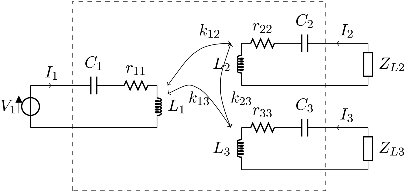
We consider a WREL system transmitting power by inductive coupling from a single transmitter to two receivers. As illustrated in Fig. 1, the structure can be schematized by means of three coupled inductors: L i with i = 1, 2, 3. We assume that a generator is present at port 1, while at port 2 and 3 we have the loads R 2 and R 3, respectively. We also assume that a compensating capacitor C i in series configuration with each inductor is present, so that the operating angular frequency ω 0 is: 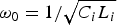 ${\omega _0} = {1 / {\sqrt {{C_i}{L_i}}}} $. In addition, we take into account losses by means of an equivalent series resistances r ii related to the respective quality factors Q i by the standard relationships Q i = ω 0L i/r ii.
Three–port network showing one transmitter at port 1 and two receivers at port 2 and 3.

In this paper we will consider the coupling between resonator i and the resonator j expressed by M ij as
 $${M_{ij}} = {k_{ij}}\sqrt {{L_i}{L_j}}, $$
where the terms k ij are the coupling coefficients and ω is the angular frequency. In the following part of this paper both the case of uncoupled receivers (i.e. k 23 = 0) and the case where a coupling between the two receivers is present (i.e. k 23 ≠ 0) will be considered.
B) Desired solutions
Let us denote with P 2 and P 3 the active power delivered to the loads on port 2 and 3. We also denote with P 1 the active power supplied to the network by the voltage source V 1. We assume that the operating frequency is  ${\omega _0} = \sqrt {{C_i}{L_i}} $ and we look for two types of solutions:
• power maximization on the loads: find the values of R 2, R 3, which maximize the total power P tot = P 2 + P 3;
• efficiency maximization: find the values of R 2, R 3, which maximize the efficiency η tot:
(2) $${\eta _{tot}} = {\eta _{12}} + {\eta _{13}},$$

where η 12 and η 13 are defined as follows:
 $$\eqalign{{\eta _{12}} =\, & \displaystyle{{{P_2}} \over {{P_1}}} \cr {\eta _{13}} =\, & \displaystyle{{{P_3}} \over {{P_1}}}.} $$
In order to find the desired solutions we will explicitly compute the relevant quantities and perform their derivatives with respect to R 2 and R 3. By setting these derivatives to zero we will find the sought value of load impedances.
III. POWER COMPUTATION AND OPTIMAL LOAD IMPEDANCES
The analysis of the circuit shown in Fig. 1 provides the following equations
 $${V_1} = \left( {{r_{11}} + j\omega {L_1} + \displaystyle{1 \over {j\omega {C_1}}}} \right){I_1} + j\omega {M_{12}}{I_2} + j\omega {M_{13}}{I_3}$$
 $$0 = j\omega {M_{12}}{I_1} + \left( {{Z_{L2}} + {r_{22}} + j\omega {L_2} + \displaystyle{1 \over {j\omega {C_2}}}} \right){I_2} + j\omega {M_{23}}{I_3}$$
 $$0 = j\omega {M_{13}}{I_1} + j\omega {M_{23}}{I_2} + \left( {{Z_{L3}} + {r_{33}} + j\omega {L_3} + \displaystyle{1 \over {j\omega {C_3}}}} \right){I_3}$$
Accordingly, the three-port network inside the dashed lines in Fig. 1 can be represented by the relation
 $${\bf V} = {{\bf Z}_{\bf 0}}{\bf I},$$
where V is the vector of port voltages, I is the vector of port currents and  ${{\bf Z}_{\bf 0}}$ is the impedance matrix, which is given by:
 $${{\bf Z}_{\bf 0}} = \quad \left( \matrix{ {{r_{11}} \!+\! j\omega {L_1}\left( {1 \!-\! \displaystyle{{\omega _0^2} \over {{\omega ^2}}}} \right)} & {j\omega {M_{12}}} & {j\omega {M_{13}}} \cr {j\omega {M_{12}}} & {{r_{22}} \!+\! j\omega {L_2}\left( {1 \!-\! \displaystyle{{\omega _0^2} \over {{\omega ^2}}}} \right)} & {j\omega {M_{23}}} \cr {j\omega {M_{13}}} & {j\omega {M_{23}}} & {{r_{33}} \!+\! j\omega {L_3}\left( {1 \!-\! \displaystyle{{\omega _0^2} \over {{\omega ^2}}}} \right)} } \right).$$
It is convenient to introduce the quantities x ij defined as:
 $${x_{ij}} = \omega {M_{ij}}{\kern 1pt}. $$
By using this definition, at the frequency of resonance ω 0,  ${{\bf Z}_{\bf 0}}$ assumes the following expression:
 $${{\bf Z}_{\bf 0}} = \left( {\matrix{ {{r_{11}}} & {j{x_{12}}} & {j{x_{13}}} \cr {j{x_{12}}} & {{r_{22}}} & {j{x_{23}}} \cr {j{x_{13}}} & {j{x_{23}}} & {{r_{33}}} \cr}} \right).$$
The vector of port voltages can be expressed as follows:
 $${\bf V} = \left( {\matrix{ {\matrix{ {{V_1}} \cr { - {R_2}{I_2}} \cr { - {R_3}{I_3}} \cr}} \cr}} \right) = \left( {\matrix{ {\matrix{ {{V_1}} \cr 0 \cr 0 \cr}} \cr}} \right) - \left( {\matrix{ 0 & 0 & 0 \cr 0 & {{R_2}} & 0 \cr 0 & 0 & {{R_3}} \cr}} \right){\bf I}{\,\rm \buildrel\textstyle.\over=\,} {\bf E} - {{\bf Z}_{\bf L}}{\bf I},$$
with obvious meaning of the symbols. By substitution into (4) we obtain:
 $${\bf E} - {{\bf Z}_{\bf L}}{\bf I} = {{\bf Z}_{\bf 0}}{\bf I},$$
or
 $${\bf I} = ({{\bf Z}_{\bf L}} + {{\bf Z}_{\bf 0}}{)^{ - 1}}{\bf E} = {\bf YE},$$
where we have introduced the admittance matrix Y.
We denote with P 1 the active power supplied by the voltage source; the active power absorbed by load i is denoted with P i and is given by
 $${P_i} = \displaystyle{1 \over 2}{R_i}{I_i}I_i^* = \displaystyle{{ \vert {V_1}{ \vert ^2}} \over 2}{R_i}{\kern 1pt} {y_{i1}}{\kern 1pt} y_{i1}^*, i = 2,3{\kern 1pt}, $$
where we have denoted with y ij the elements of the admittance matrix Y. It is convenient to introduce the following quantity
 $$\Delta = {r_{11}}{R_2}{R_3} + {r_{11}}{r_{22}}{R_3} + x_{12}^2 {R_3} + {r_{11}}{r_{33}}{R_2} + x_{13}^2 {R_2} + {r_{11}}{r_{22}}{r_{33}} + x_{12}^2 {r_{33}} + x_{13}^2 {r_{22}},$$
which allows to write the terms in the first column of the admittance matrix as
 $$\eqalign{{y_{11}} =\,\, & \displaystyle{{({R_2} + {r_{22}}){\kern 1pt} ({R_3} + {r_{33}})} \over \Delta} \cr {y_{21}} =\,\, & j\displaystyle{{{x_{12}}({R_3} + {r_{33}})} \over \Delta} \cr {y_{31}} =\,\, & j\displaystyle{{{x_{13}}{\kern 1pt} ({R_2} + {r_{22}})} \over \Delta}.} $$
It is also convenient to introduce the normalized powers P i defined as
 $${p_i} = \displaystyle{{8{r_{11}}{P_i}} \over { \vert {V_1}{ \vert ^2}}}{\kern 1pt}. $$
With the above definitions the power values are given by
 $$\eqalign{{p_1} =\, & 4{r_{11}}\displaystyle{{({R_2} + {r_{22}}){\kern 1pt} ({R_3} + {r_{33}})} \over \Delta} \cr {p_2} =\, & 4{r_{11}}\displaystyle{{x_{12}^2 \;{R_2}{{({R_3} + {r_{33}})}^2}} \over {{\Delta ^2}}} \cr {p_3} =\, & 4{r_{11}}\displaystyle{{x_{13}^2 \;{{({R_2} + {r_{22}})}^2}\;{R_3}} \over {{\Delta ^2}}}.} $$
A) Maximum power solution
In this section the problem of power maximization is addressed. The value of the load impedances, which allows to maximize the power delivered at port 2 and 3 is determined both in the case of coupled and uncoupled receivers. Note that in the case of coupled receivers the analytical complexity prevents to solve the problem in closed form. Nonetheless, by using appropriate reactive elements we can still retrieve the same results as in the uncoupled case.
1) The case of uncoupled receivers
We start our analysis by considering the case, where no coupling is present between the two receivers (i.e. resonators 2 and 3). In this case, the terms Z 0,23 and Z 0,32 of the impedance matrix  ${{\bf Z}_{\bf 0}}$ are equal to zero (i.e. x 23 = 0), and (7) simplifies as follows:
 $${{\bf Z}_{\bf 0}} = \left( {\matrix{ {{r_{11}}} & {j{x_{12}}} & {j{x_{13}}} \cr {j{x_{12}}} & {{r_{22}}} & 0 \cr {j{x_{13}}} & 0 & {{r_{33}}} \cr}} \right).$$
In order to better express the solutions it is convenient to introduce the following definitions:
 $$\eqalign{\chi _{12}^2 =\, & \displaystyle{{x_{12}^2} \over {{r_{11}}{\kern 1pt} {r_{22}}}} = k_{12}^2 {Q_1}{Q_2} \cr \chi _{13}^2 =\, & \displaystyle{{x_{13}^2} \over {{r_{11}}{\kern 1pt} {r_{33}}}} = k_{13}^2 {Q_1}{Q_3} \cr \chi _{23}^2 =\, & \displaystyle{{x_{23}^2} \over {{r_{22}}{\kern 1pt} {r_{33}}}} = k_{23}^2 {Q_2}{Q_3} \cr \theta \,=\, & \sqrt {\left( {1 + \chi _{12}^2 + \chi _{13}^2} \right)}.} $$
It is feasible, by using a computer algebra system, to perform the derivatives of the total power P tot = P 2 + P 3 with respect to R 2, R 3, equating them to zero and solving the system. The rather long expressions are not reported here. By doing this procedure we have obtained six solutions, but only one is meaningful since five solutions refer to negative resistance values. The load resistances that realize maximum power transfer are:
 $$\eqalign{& {{R_{2}^{\prime}}} = {r_{22}}{\kern 1pt} {\theta ^2} \cr & {{R_{3}^{\prime}}} = {r_{33}}{\kern 1pt} {\theta ^2}{\kern 1pt},} $$
where we have used the prime in order to refer to the maximum power solutions. It is noted that this result nicely extends the one obtained in [Reference Dionigi, Mongiardo and Perfetti24]. Note that when the results in (18) are inserted into (13) we recover the following expressions
 $$\eqalign{{y_{11}} =\, & \displaystyle{{{\theta ^2} + 1} \over {2{\kern 1pt} {r_{11}}{\kern 1pt} {\theta ^2}}} \cr {y_{21}} =\, & - j\displaystyle{{{\chi _{12}}} \over {2\sqrt {{r_{11}}{r_{22}}} {\theta ^2}}} \cr {y_{31}} =\, & - j\displaystyle{{{\chi _{13}}} \over {2\sqrt {{r_{11}}{r_{33}}} {\theta ^2}}}.} $$
2) The case of coupled receivers
Let us now consider the case of coupled receivers (i.e. k 23 ≠ 0). This case differs from the previous one because of the terms Z 0,23 and Z 0,32 of the impedance matrix  ${{\bf Z}_{\bf 0}}$ that are now different from zero and depend on the coupling between port 2 and port 3. In more detail, in the coupled case the three ports network is described by the impedance matrix
 ${{\bf Z}_{\bf 0}}$ as given in (7); it can be seen that at the frequency of resonance Z 0,23 and Z 0,32 are purely imaginary. As a consequence, we can infer that:
• the values of the resistances R′2, R′3 remain the same as found for the uncoupled case;
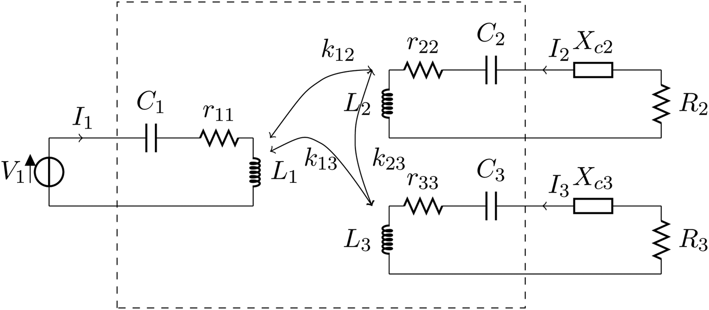
• we need to add two compensating series reactances X′c2, X′c3, as shown in Fig. 2, in order to maximize power.
Fig. 2.When the cross-coupling term k 23 is different from zero, it is still possible to add the compensating reactances X c2, X c3 that allows to retrieve the same results of the uncoupled case. The compensating reactances are the same for the maximum efficiency and maximum power transfer cases so that X″c2 = X′c2 = X c2, X″c3 = X′c3 = X c3.
In particular, the values of these compensating reactances are:
 $$\eqalign{{{X_{c2}^{\prime}}} = & - \displaystyle{{{x_{13}}{x_{23}}} \over {{x_{12}}}}\displaystyle{{{r_{22}}} \over {{r_{33}}}} \cr {{X_{c3}^{\prime}}} = & - \displaystyle{{{x_{12}}{x_{23}}} \over {{x_{13}}}}\displaystyle{{{r_{33}}} \over {{r_{22}}}}.} $$
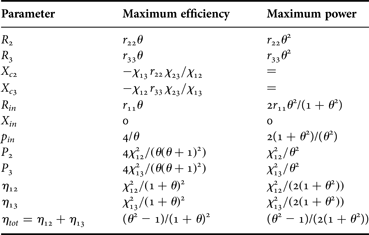
Note that when inserting the above elements in our network we recover again the admittances reported in (19). In fact, from a practical point of view, the purpose of these reactances is to compensate for the presence of a coupling between the two receivers, thus making the coupled case identical to the uncoupled one; so that, we recover the same solution for the load impedances. By using the values given in (18) and in (20) we get the corresponding input impedance, normalized powers and efficiencies as reported in Table 1.
A summary of the parameters values for the approaches that maximize efficiency and power.
The powers have been normalized with respect to  ${P_0} = {{V_1^2} / {(8{r_{11}})}}$. R in and X in are the real and the imaginary part of the input impedance (Z in) as seen from the generator (i.e. Z in = R in + jX in). p in is the normalized input power. The parameters have the following meanings:
 ${\chi _{12}} = {{{x_{12}}} / {\sqrt {{r_{11}}{r_{22}}}}} $,
 ${\chi _{13}} = {{{x_{13}}} / {\sqrt {{r_{11}}{r_{33}}}}} $,
 ${\chi _{23}} = {{{x_{23}}} / {\sqrt {{r_{22}}{r_{33}}}}} $,
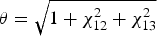 $\theta = \sqrt {1 + \chi _{12}^2 + \chi _{13}^2} $.
B) Maximum efficiency solution
In this section we look for the load impedances R 2 and R 3, which allow to maximize the efficiency as defined in (2).
1) The case of uncoupled receivers
This time, using again a computer algebra system, we have computed the derivatives of the efficiency defined in (2) with respect to R 2, R 3; we have equated them to zero and solved the system. The rather long expressions are not reported here. By doing this procedure we have obtained three possible solutions, with only one meaningful, since the other two solutions refer to negative impedance values. The load impedances, which maximize efficiency are:
 $$\eqalign{& {{R_{2}^{\prime \prime}}} = {r_{22}}\theta \cr & {{R_{3}^{\prime \prime}}} = {r_{33}}\theta,} $$
where we have used the double prime in order to refer to the maximum efficiency solution. It is noted that also this result extends the one obtained in [Reference Dionigi, Mongiardo and Perfetti24]. When using the values of (21) into (13) we obtain
 $$\eqalign{{y_{11}} =\, & \displaystyle{1 \over {{r_{11}}{\theta ^2}}} \cr {y_{21}} = & - j\displaystyle{{{\chi _{12}}} \over {2\sqrt {{r_{11}}{r_{22}}} (\theta (\theta + 1))}} \cr {y_{31}} = & - j\displaystyle{{{\chi _{13}}} \over {2\sqrt {{r_{11}}{r_{33}}} (\theta (\theta + 1))}}.} $$
2) The case of coupled receivers
We are not able to solve the maximum efficiency case when x 23 ≠ 0. In this regard, it is worth observing that in [Reference Dionigi, Mongiardo and Perfetti24] it was demonstrated that the compensating reactances to be added for maximum power or for maximum efficiency, are the same. Can we extend this result to the two receivers case? When we insert the compensating reactances given in (20) we retrieve the same results for powers in both the coupled and the uncoupled case, is this true also for the efficiency?
It can be demonstrated that the answer is positive for the special cases of the loads corresponding to maximum efficiency and maximum power solution. More in general, it can be demonstrated that the compensating reactances allow to retrieve the same results for powers and efficiency when the load impedances at port 2 and at port 3 satisfy the following relations:
 $$\eqalign{& {R_2} = {r_{22}}l \cr & {R_3} = {r_{33}}l{\kern 1pt},} $$
being l a constant.
This result can be demonstrated as follows. Let us write the impedance matrix of the network in the case of coupled receivers and when the compensating reactances expressed in (20) are present:
 $${{\bf Z}_{\bf c}} = \left( {\matrix{ {{r_{11}}} & {j{x_{12}}} & {j{x_{13}}} \cr {j{x_{12}}} & {{r_{22}} - j\displaystyle{{{x_{13}}{x_{23}}} \over {{x_{12}}}}\displaystyle{{{r_{22}}} \over {{r_{33}}}}} & {j{x_{23}}} \cr {j{\kern 1pt} {x_{13}}} & {j{\kern 1pt} {x_{23}}} & {{r_{33}} - j\displaystyle{{{x_{12}}{x_{23}}} \over {{x_{13}}}}\displaystyle{{{r_{33}}} \over {{r_{22}}}}} \cr}} \right).$$
From (9) and (24) we can derive that the admittance matrix ( ${{\bf Y}_{\bf c}}$) is given by:
 $${{\bf Y}_{\bf c}} = ({{\bf Z}_{\bf L}} + {{\bf Z}_{\bf c}}{)^{ - 1}} = {\left( {\matrix{ {{r_{11}}} & {j{x_{12}}} & {j{x_{13}}} \cr {j{x_{12}}} & {{r_{22}} + {R_2} + j{X_{c2}}} & {j{x_{23}}} \cr {j{x_{13}}} & {j{x_{23}}} & {{r_{33}} + {R_3} + j{X_{c3}}} \cr}} \right)^{ - 1}}.$$
From (20), (25), and (23) it can be verified that the following equalities hold:
 $$\eqalign{{y_{c,11}} =\, & {y_{11}} \cr {y_{c,21}} =\, & {y_{21}} \cr {y_{c,31}} =\, & {y_{31}}.} $$
As a consequence, we can conclude that when the loads at port 2 and at port 3 satisfy (23), the addition of the compensating reactances expressed in (20) allows to retrieve the same powers and efficiency for both the coupled and the uncoupled case.
From (21) and (18) it can be seen that both the load resistances that maximize power and the ones that maximize efficiency satisfy (23), therefore we can assert that, using the optimal loads, power and efficiency are the same with or without coupling k 23, provided that reactances (20) are inserted.
According to the above reported considerations, we derived the maximum efficiency solution for the coupled case by introducing the compensating reactances X″c2 = X′c2 = X c2, X″c3 = X′c3 = X c3, this way we have recovered the values reported in Table 1.
C) Discussion of the results
By comparing results reported in the previous part of this section with those reported in [Reference Dionigi, Mongiardo and Perfetti24], where the same problem is solved for a single-receiver system, we note that the introduction of an additional receiver changes the optimal load impedance. In particular, the load impedance is increased. Therefore, when a system with multiple loads is designed, one should take into account that the optimal impedance should be changed when a further receiver is present.
It is also noted that the solution, which delivers maximum power to the load always presents a larger resistance value with respect to the solution, which provides maximum efficiency. It is this range, i.e. R″2 >R 2 >R′2, R″3 >R 3 >R′3, which is the most interesting one for the selection of the load impedances.
IV. NUMERICAL RESULTS
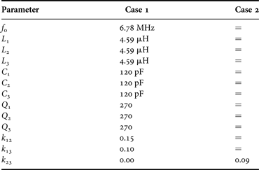
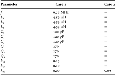
In order to illustrate the proposed approach, two numerical examples have been selected as illustrated in Table 2. Both examples refer to a two receivers WREL and differ only in the mutual coupling between the receivers: in the first example the receivers are not coupled (i.e. k 23 = 0), while in the second example the two receivers are coupled (i.e. k 23 ≠ 0). The parameters corresponding to the two examples are gathered in the second column (case 1) and in the third column (case 2) of Table 2.
Two cases of three coupled resonators: for case 1 (k 23 = 0), the terminating impedances are purely resistive. For case 2, all the couplings are considered and the terminating impedances become complex.
Using these values, we obtain the following impedance matrix:
 $$Z = \left( {\matrix{ {50.724 \, \Omega} & {j29.33 \, \Omega} & {j19.553 \, \Omega} \cr {j29.33 \, \Omega} & {0.7242 \, \Omega} & {j{x_{23}}} \cr {j19.553 \, \Omega} & {j{x_{23}}} & {0.7242 \, \Omega} \cr}} \right),$$
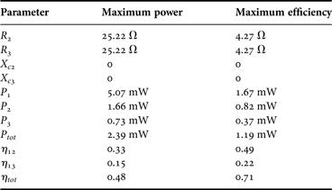
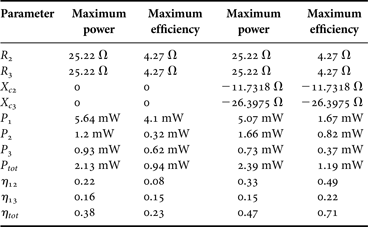
where the parameter x 23 is equal to zero for case 1, while it is equal to −17.6 Ω for case 2. By applying the formulas reported in Table 1 we obtain the results listed in Table 3 for case 1. It can be noticed that the impedances that realize maximum power transfer are greater than the ones that realize maximum efficiency. The results corresponding to the case, where the receivers are coupled (i.e. case 2 of Table 2) are given in Table 4. The first two columns illustrate the results calculated when the compensating reactances are not present, while the last two columns illustrate the results calculated by adding the compensating reactances X c2 = −11.7318 Ω and X c3 = −26.3975 Ω, which correspond to two series capacitances C 2 = 2 nF and C 3 = 889.26 pF. From the first two columns of Table 4, it can be noticed that the presence of a coupling between the two receivers affects both the power on the loads and the efficiency. Additionally, it is evident that the efficiency is more sensitive than power to this coupling; in fact, the total efficiency lowers from 0.71 to 0.23. By comparing the last two columns of Table 4 with Table 3, it can be derived that the addition of the compensating reactances allows retrieving the same results calculated for the uncoupled case for both the power on the loads and the efficiency, thus validating the analytical formulas derived in the previous section.
Results for three coupled resonators: the element values are listed in Table 2 and refer to case 1. We have assumed that a 1 V generator is present at port 1. It has also been assumed that the generator presents an internal impedance of 50 Ω which has been included in r 11.
Results for three coupled resonators: the element values are listed in Table 2 and refer to case 2. We have assumed that a 1 V generator is present at port 1. It has also been assumed that the generator presents an internal impedance of 50 Ω, which has been included in r 11. The first two columns illustrate the results calculated for case 2 without the compensating reactances X c2 and X c3, while the last two columns illustrate the results calculated by adding the compensating reactances X c2 and X c3.
In order to verify results summarized in Table 3 and 4, circuital simulations have been performed by using the commercial tool NI AWR design environment. Corresponding results are given in Figs 3–9. Figures 3–6 refer to case 1; in more detail, Figs 3 and 5 illustrate results obtained for the active power delivered to the loads (i.e. P 2, P 3, and P tot), while Figs 4 and 6 illustrate results obtained for the efficiency. Circuital simulations confirm that the values of the load impedances, which maximize power and efficiency are the ones given in Table 3, thus validating (18) and (21).
Power for case 1 as a function of R 2 and R 3. (a) Power on the load at port 2 (i.e. power dissipated on the resistance R 2). (b) Power on the load at port 3 (i.e. power dissipated on the resistance R 3). The results have been obtained by circuit simulations by varying the values of the loads R 2 and R 3. The numeric values on the contour lines indicate the values of the power in mW.
Efficiency for case 1 as a function of the loads R 2 and R 3. (a) Efficiency with respect to the load at port 2 (i.e. η 12). (b) Efficiency with respect to the load at port 3 (i.e. η 13). The results have been obtained by circuit simulations by varying the values of the loads R 2 and R 3. The numeric values on the contour lines indicate the values of the efficiency.
Total power for case 1 calculated by circuit simulations by varying the values of the loads R 2 and R 3. The numeric values on the contour lines indicate the values of the total power in mW.
Efficiency for case 1 calculated by circuit simulations by varying the values of the loads R 2 and R 3. The numeric values on the contour lines indicate the values of the efficiency.
Total power for case 2 calculated by circuit simulations by varying the values of the loads R 2 and R 3. The numeric values on the contour lines indicate the values of the total power in mW.
Efficiency for case 1 calculated by circuit simulations by varying the values of the loads R 2 and R 3. The numeric values on the contour lines indicate the values of the efficiency.
Difference between the total powers calculated for case 1 and case 2 by varying the values of the loads R 2 and R 3.
Results obtained for case 2 are given in Figs 7 and 8; also in the coupled case circuital simulations are in a perfect agreement with data summarized in Table 4, thus validating theoretical results reported in the previous section. In particular, circuital simulations for case 2 were performed by adding the compensating reactances X c2 and X c3 (see Table 4), results obtained this way confirm that these reactances allow to recover in the coupled case the same results obtained for the uncoupled case when the load impedances are the ones for power or efficiency maximization. This result is highlighted in Figs 9 and 10, where the difference between results obtained for case 1 and case 2 are illustrated. In more details, the figures show the quantities P diff and η diff, which are defined as the absolute value of the difference between the values calculated for case 1 and case 2 for the total power and the total efficiency, respectively. It can be seen that this difference is negligible in regions with maximum power or maximum efficiency.
Difference between the total efficiencies calculated for case 1 and case 2 by varying the values of the loads R 2 and R 3.
Finally, in order to investigate the dependence of the results reported in Figs 3–8 on possible variations of the couplings among the resonators, a sensitivity analysis has been performed.
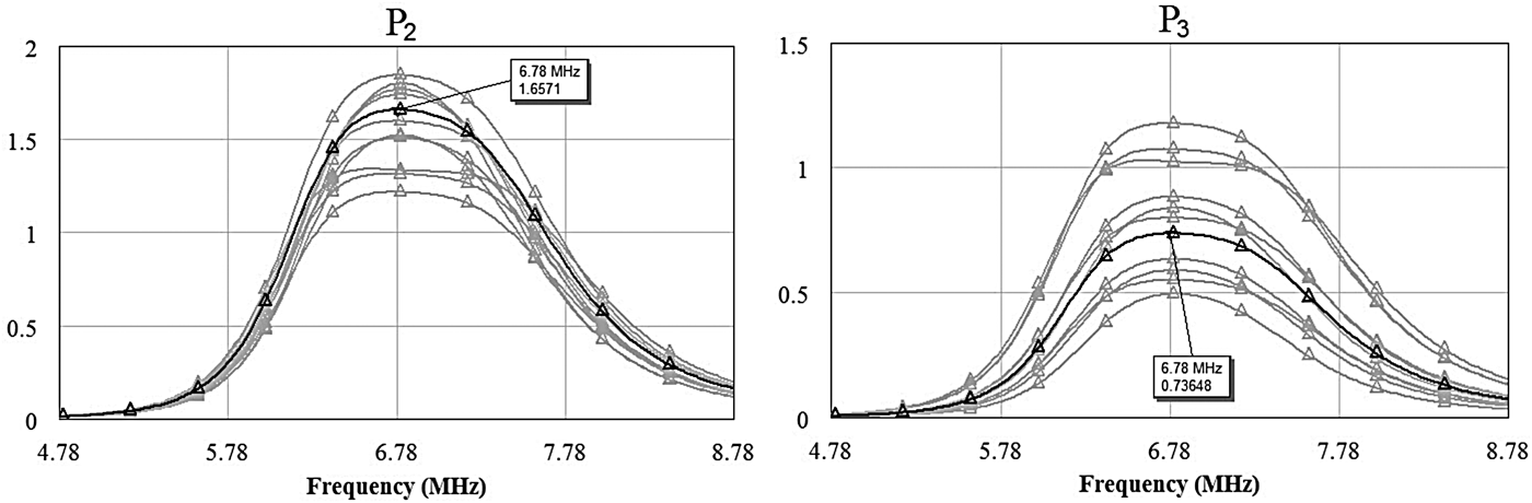
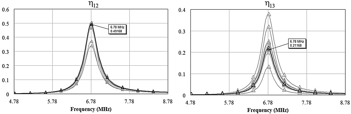
More specifically, we assumed for both the k 12 and the k 13 parameters a uniform distribution with a 20% standard deviation from their nominal values. Accordingly, circuit simulations have been performed by randomly varying the k 12 parameter in the range (0.12, 0.18) and the k 13 parameter in the range (0.08, 0.12).
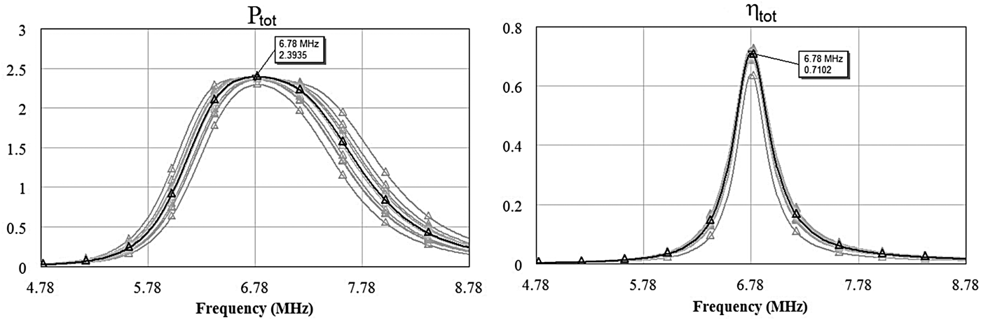
Results obtained for the case of uncoupled receivers (i.e. k 23 = 0) are summarized in Figs 11–13. As it can be seen, with respect to the values calculated at the nominal values of k 12 and k 13, a large variation has been obtained for the efficiencies η 12 and η 13 and the powers P 2 and P 3, while a more robust behavior has been obtained for the total efficiency η tot and the total power P tot.
Sensitivity analysis results calculated by circuit simulations for the powers P 2 and P 3. The values assumed for the loads are the ones corresponding to power maximization (i.e. R L2 = R L3 = 25.22 Ω). The black curves are the results calculated by setting the couplings k 12 and k 13 at their nominal values (i.e. k 12 = 0.15 and k 13 = 0.1), whereas the gray curves are the results obtained by randomly varying k 12 in the range (0.12, 0.18) and k 13 in the range (0.08, 0.12). The powers are in mW.
Sensitivity analysis results calculated by circuit simulations for the efficiencies η 12 and η 13. The values assumed for the loads are the ones corresponding to efficiency maximization (i.e. R L2 = R L3 = 4.27 Ω). The black curves are the results calculated by setting the couplings k 12 and k 13 at their nominal values (i.e. k 12 = 0.15 and k 13 = 0.1), whereas the gray curves are the results obtained by randomly varying k 12 in the range (0.12, 0.18) and k 13 in the range (0.08, 0.12).
Sensitivity analysis results calculated by circuit simulations for the total power P tot (on the left) and the total efficiency η tot (on the right). Results referring to P tot have been calculated by using for R L2 and R L3 the values corresponding to power maximization (i.e. R L2 = R L3 = 25.22 Ω), while results referring to η tot have been calculated by using for R L2 and R L3 the values corresponding to efficiency maximization (i.e. R L2 = R L3 = 4.27 Ω). The black curves are the results calculated by setting the couplings k 12 and k 13 at their nominal values (i.e. k 12 = 0.15 and k 13 = 0.1), whereas the gray curves are the results obtained by randomly varying k 12 in the range (0.12, 0.18) and k 13 in the range (0.08, 0.12). Results reported for the power are in mW.
V. CONCLUSION
The problem of magnetic resonant wireless power transfer between one transmitter and two loads has been considered from a rigorous network viewpoint. Given the network parameters, the problem of maximizing either the power on the loads or the efficiency has been analytically solved. With respect to the use of a circuit simulator to solve the same problem, the main advantages of the proposed analysis is that it provides closed form formulas for the optimal loads, which can be used in order to evaluate the sensitivity of the link performance on the network parameters.
Both cases of coupled and uncoupled receivers have been considered; it has been demonstrated that in the case of coupled receivers the addition of appropriate compensating reactances allows retrieving the same results corresponding to the uncoupled case.
Two numerical simulations have been selected and calculated. The results have indicated that, by introducing an additional receiver, the optimal load impedances (both for maximum efficiency and for maximum power transfer) are changed.
Giuseppina Monti Giuseppina Monti received the Laurea degree in Telecommunication Engineering (with honors) from the University of Bologna, Italy, in 2003, and the Ph.D. in Information Engineering from University of Salento (Italy), in 2007. She is currently with the Department of Innovation Engineering (University of Salento), where she is a temporary researcher and lecturer in CAD of Microwave circuits and Antennas. Her current research interest includes the analysis and applications of artificial media (such as, for instance, double-negative metamaterials and nano-carbontube), the analysis of electromagnetic compatibility and electromagnetic interference problems in planar microwave circuits, the design and realization of: microwave components and MEMS-based reconfigurable antennas and devices, rectenna systems, systems and devices for wireless power transmission applications. She has co-authored a chapter of a book and about 100 papers appeared in international conferences and journals.
Wen Quan Che Wen Quan Che (M-01–SM-11) received the B.Sc. degree from the East China Institute of Science and Technology, Nanjing, China, in 1990, the M.Sc. degree from the Nanjing University of Science and Technology (NUST), Nanjing, China, in 1995, and the Ph.D. degree from the City University of Hong Kong (CITYU), Kowloon, Hong Kong, in 2003. In 1999, she was a Research Assistant with the City University of Hong Kong. From March to September 2002, she was a Visiting Scholar at the Polytechnique de Montreal, Montreal, QC, Canada. She is currently a Professor at the Nanjing University of Science and Technology, Nanjing, China. From 2007 to 2008, she conducted academic research with the Institute of High Frequency Technology, Technische Universitaet Muenchen. During the summers of 2005–2006 and 2009–2013, she was with the City University of Hong Kong, as Research Fellow and Visiting Professor. She has authored or coauthored over 120 internationally referred journal papers and over 60 international conference papers. She has been a reviewer for IET Microwaves, Antennas and Propagation. Her research interests include electromagnetic computation, planar/coplanar circuits and subsystems in RF/microwave frequency, microwave monolithic integrated circuits (MMICs) and medical application of microwave technology. Dr. Che has been a reviewer for the IEEE transactions on microwave theory and techniques, IEEE transactions on antennas and propagation, IEEE transactions on industrial electronics, and IEEE microwave and wireless components letters. She was the recipient of the 2007 Humboldt Research Fellowship presented by the Alexander von Humboldt Foundation of Germany, the 5th China Young Female Scientists Award in 2008, and the recipient of Distinguished Young Scientist award by the National Natural Science Foundation Committee (NSFC) of China in 2012.
Qinghua Wang Qinghua Wang was born in Jiangsu Province; China in 1993. She received the B.Sc. degree in 2014 from Nanjing University of Science and Technology (NUST), Nanjing, China. She is currently working towards the Ph.D. degree at NUST. Her research interest is mainly on wireless power transmission.
Marco Dionigi has received the laurea degree (110/110 cum laude) in Electronic Engineering from the University of Perugia. He achieved at the same university the title of Ph.D. In 1997 he became Assistant Professor at the Faculty of Engineering of the University of Perugia. He took part in several research project regarding the development of software tools for waveguide and antenna fullwave simulation, the development of permittivity and moisture microwave sensors, the development of a SAR and ultrawideband antennas. He was coauthor of a paper awarded of the “Young Engineers Prize” at the European Microwave Conference 2005 in Paris. He is now involved in the study and development of high efficient wireless electromagnetic power transfer for industrial applications. He is author of more than 70 papers on international journal and conferences.
Mauro Mongiardo received the laurea degree (110/110 cum laude) in Electronic Engineering from the University of Rome “La Sapienza” in 1983. In 1991 he became Associate Professor of Electromagnetic Fields and from 2001 he is Full Professor of Electromagnetic Fields at the University of Perugia. He has been elected Fellow of the IEEE “for contributions to the modal analysis of complex electromagnetic structures” in 2013. His scientific interests concern primarily the numerical modeling of electromagnetic wave propagation both in closed and open structures. His research interests involve CAD and optimization of microwave components and antennas. He has served in the Technical Program Committee of the IEEE International Microwave Symposium from 1992; from 1994 he is the member of the Editorial Board of the IEEE transactions on microwave theory and techniques. During the years 2008–2010 he has been Associate Editor of the IEEE transactions on microwave theory and techniques. He is author or co-author of over 200 papers and articles in the fields of microwave components, microwave CAD and antennas. He is the co-author of the books “Open Electromagnetic Waveguides” (IEE, 1997), and “Electromagnetic Field Computation by Network Methods” (Springer, 2009). Recently, he has co-authored a chapter in the book Wireless Power Transfer – Principles and Engineering Explorations (Intech, 2012), and a chapter in the book Wireless Power Transfer (River publishers, 2012).
Renzo Perfetti received the laurea degree with honors in Electronic Engineering from the University of Ancona, Italy, in 1982, and the Ph.D. degree in Information and Communication Engineering from the University of Rome “La Sapienza” in 1992. From 1983 to 1987 he was with the radar division of Selenia, in Rome, where he worked on radar systems design and simulation. From 1987 to 1992 he was with the radiocommunication division of Fondazione U. Bordoni in Rome. In 1992 he joined the Department of Electronic and Information Engineering of the University of Perugia, Italy, where he is currently a Full Professor of electrical engineering. His current research interests include circuit theory, machine learning, audio and biomedical signal processing.
Yumei Chang Yumei Chang (M-12) was born in Hebei Province, China, in 1983. She received the M. Sc. degree in 2009 and the Ph.D. degree in 2014 from the Nanjing University of Science and Technology (NUST), Nanjing, China. From September 2012 to February 2013, she was a visiting scholar in the department of Electronic and Computer Engineering at University of Waterloo, Canada. She has authored or coauthored over 10 journal and conference papers. Her research interests include wireless power transmission, microwave absorbers, FSS and microwave/millimeter-wave devices.