

1 Introduction
A large number of research studies have been devoted to enhance the understanding of flow-induced vibration (FIV) of structures due to its practical importance to engineering. FIV is a vibration phenomenon of solid structures induced by the flow of the surrounding fluid. When a fluid flows past a bluff solid structure, a large-amplitude fluctuation pressure force develops near the rear of the structure, which leads to the formation of a wake with alternately shedding vortices. Moreover, when the vortex formation frequency is matched by the system’s natural frequency, the response is termed vortex-induced vibration (VIV). This is a highly periodic vibration state that can be sustained over a lengthy period. Fatigue damage or failure of a structure can be caused by FIV and, therefore, it is a crucial consideration for the design of many engineering systems. Some examples are bridges, chimney stacks, aircraft, ground vehicles, submarines, tethered structures and offshore structures. Hence, it is important to improve our understanding of FIV and the methods of controlling it.
The field of FIV has been continuously developing over the last few decades through experimental and computational studies. Its fundamentals have been revealed substantially through the study of basic geometries. Indeed, many books have been devoted to the field; the reader is referred to the textbook of Blevins (Reference Blevins1977) for a detailed introduction. The comprehensive reviews of Bearman (Reference Bearman1984), Parkinson (Reference Parkinson1989), Sarpkaya (Reference Sarpkaya2004), Williamson & Govardhan (Reference Williamson and Govardhan2004, Reference Williamson and Govardhan2008) and Wu, Ge & Hong (Reference Wu, Ge and Hong2012) provide further insight. Most of the studies have been based on cylindrical structures, albeit there are ample applications with spherical geometries. For example, tethered bodies such as buoys, underwater mines, tethered balloons and towed objects behind vessels are often spherical.
The majority of early studies of tethered spheres have concerned the effect of surface waves on tethered buoyant spheres. For example, the investigations of Harleman & Shapiro (Reference Harleman and Shapiro1960) and Shi-Igai & Kono (Reference Shi-Igai and Kono1969) employed ‘Morison’s equation’ and empirically obtained drag and inertial coefficients to predict the FIV of the sphere as a forced vibration problem. The coupling of wave motion and the sphere dynamics yielded a complicated equation for which the underlying controlling physics is difficult to understand. Gottlieb (Reference Gottlieb1997) investigated the response of a nonlinear small-body ocean-mooring system excited by finite-amplitude waves and restrained by a massless elastic tether. He determined the stability of periodic motion numerically using Floquet analysis and found that the bifurcation structure includes ultra-subharmonic and quasi-periodic responses. The hydrodynamic dissipation mechanism was found to control stability thresholds, whereas the convective nonlinearity governed the evolution to a chaotic system response.
Vortex-induced vibration of a tethered sphere in a uniform flow was first studied by Williamson & Govardhan (Reference Williamson and Govardhan1997) and Govardhan & Williamson (Reference Govardhan and Williamson1997) experimentally. They discovered that a tethered sphere vibrates vigorously at a saturation amplitude of close to two diameters peak-to-peak. Moreover, the sphere oscillation increased the drag force and the tether angle by the order of  $100\,\%$ over that predicted using the drag measurement of a stationary sphere. The transverse oscillation frequency was half that of the streamwise oscillation frequency, despite the fact that the natural frequency of a tethered body is independent of the direction. They observed an excellent collapse of data over a range of different mass ratios (the density ratio between the sphere and fluid,
 $m^{\ast }$) and tether length ratios (the ratio between tether length and the sphere diameter,
 $l^{\ast }$) when plotting the sphere response amplitude versus reduced velocity,
 $U^{\ast }=U/(f_{n}D)$, rather than versus Reynolds number, where
 $U$ is the upstream velocity,
 $f_{n}$ is the natural frequency of the system and
 $D$ is the diameter of the sphere.
Govardhan & Williamson (Reference Govardhan and Williamson1997) observed a local peak in the amplitude response curve when the root-mean-square (r.m.s.) value of the amplitude was used instead of the maximum amplitude. This peak appeared around  $U^{\ast }\sim 6$. It was further found that the vortex shedding frequency,
 $f_{s}$, matched the system’s natural frequency,
 $f_{n}$, and the vortex shedding frequency of the static sphere,
 $f_{vo}$. Indeed, this is a VIV response caused by resonance and is known as mode I vibration. After mode I, as the reduced velocity is increased, Jauvtis, Govardhan & Williamson (Reference Jauvtis, Govardhan and Williamson2001) and Govardhan & Williamson (Reference Govardhan and Williamson2005) observed another periodic VIV response known as mode II vibration. The amplitude of the mode II was approximately twice that of mode I. The transition between these two modes was quite distinct for very light tethered bodies (
 $m^{\ast }<1$). However, for elastically mounted higher-mass-ratio spheres, the transition between modes I and II was more continuous in the amplitude response curve. By analysing force measurements, Govardhan & Williamson (Reference Govardhan and Williamson2005) showed that the phase of the vortex force relative to the sphere motion was approximately
 $90^{\circ }$ higher for mode II compared to mode I. They observed a chain of two-sided hairpin vortex loops in the wake for both modes I and II with aid of digital particle image velocimetry (DPIV).
Hout, Krakovich & Gottlieb (Reference Hout, Krakovich and Gottlieb2010) identified three bifurcation regions for VIV of a heavy ( $m^{\ast }=7.87$) tethered sphere in the reduced velocity range,
 $2.8\leqslant U^{\ast }\leqslant 31$. The sphere remained stationary in the first regime while it showed large-amplitude periodic oscillations in the second regime. Consistent with the observation of Govardhan & Williamson (Reference Govardhan and Williamson2005), they also found that the phase at which vortices were shed increased with increasing
 $U^{\ast }$ in the second bifurcation region. In the third bifurcation regime, the sphere showed less-periodic and smaller-amplitude vibration.
For VIV of a cylinder, it has been discovered that a critical mass ratio,  $m_{crit}^{\ast }$, exists, below which a large-amplitude response will persist up to infinite reduced velocity. Using the effective added mass, Govardhan & Williamson (Reference Govardhan and Williamson2005) estimated that
 $m_{crit}^{\ast }$ is approximately
 $0.6$ for a sphere. Eshbal, Krakovich & Hout (Reference Eshbal, Krakovich and Hout2012) investigated the VIV of a light tethered sphere with
 $m^{\ast }<m_{crit}^{\ast }$, for the Reynolds-number range
 $430\leqslant Re\leqslant 1925$. As
 $U^{\ast }$ increased, they observed a continuously increasing trend in the r.m.s. amplitudes after the first bifurcation, as expected.
Coulombe-Pontbriand & Nahon (Reference Coulombe-Pontbriand and Nahon2009) investigated the dynamics of spherical aerostat on a single tether in the supercritical Reynolds-number range ( $Re>3.7\times 10^{5}$). Their experiments demonstrated that a tethered sphere in a turbulent flow will strongly oscillate. The amplitude of the transverse oscillation was found to increase with the increasing
 $U^{\ast }\in [5{-}40]$ but was independent of the tether length. Moreover, they found that there was a substantial increment in the drag coefficient of the balloon due to its large oscillations, surface roughness and wind turbulence, consistent with the result of Govardhan & Williamson (Reference Govardhan and Williamson1997).
Jauvtis et al. (Reference Jauvtis, Govardhan and Williamson2001) experimentally found another periodic large-amplitude vibration state beyond the mode II regime, with heavy spheres of mass ratios  $m^{\ast }=28$,
 $80$ and
 $940$. It appeared in the reduced velocity range
 $U^{\ast }\sim 20{-}40$ and was named mode III. It was difficult to explain the cause of mode III using classic lock-in theories, since the principal vortex shedding frequency was found to be 3–8 times higher than the sphere vibration frequency. Later, Govardhan & Williamson (Reference Govardhan and Williamson2005) classified mode III as a movement-induced excitation. However, the nature of the mode III vibration state has not been examined in detail and further investigations seem warranted to enhance the understanding of this mode. Subsequently, Jauvtis et al. (Reference Jauvtis, Govardhan and Williamson2001) found another vibration state after mode III for
 $U^{\ast }>100$ with a sphere of
 $m^{\ast }=80$, which is known as mode IV. In this mode, the sphere showed intermittent bursts of vibrations, in contrast to (near-)periodic vibrations for the first three modes. Despite being an aperiodic vibration, interestingly, the main frequency component was close to the natural frequency of the system. Moreover, it was observed that the response amplitude increased with increasing reduced velocity.
Behara, Borazjani & Sotiropoulos (Reference Behara, Borazjani and Sotiropoulos2011) investigated VIV with an elastically mounted sphere computationally, allowing three degrees of freedom of motion, at Reynolds number of  $Re=300$ and reduced mass of
 $m_{r}=2$. Over the reduced velocity range,
 $4\leqslant U^{\ast }\leqslant 9$, they observed two distinct sphere vibration modes at the same reduced velocities, namely hairpin and spiral modes. More recently, Behara & Sotiropoulos (Reference Behara and Sotiropoulos2016) extended this study by expanding the
 $U^{\ast }$ range and increasing the Reynolds number up to
 $1000$ at
 $U^{\ast }=9$. They identified that the hairpin mode is unstable and merges with the spiral mode at
 $U^{\ast }=9$. Moreover, the detailed sphere response was found to be strongly dependent on the Reynolds number.
The combined experimental and numerical studies of Lee, Hourigan & Thompson (Reference Lee, Hourigan and Thompson2013) on the VIV of a neutrally buoyant ( $m^{\ast }=1$) tethered sphere covered the Reynolds-number range
 $50\leqslant Re\leqslant 12\,000$. They identified seven different broad but relatively distinct oscillation and wake states. The more recent study of Rajamuni, Thompson & Hourigan (Reference Rajamuni, Thompson and Hourigan2018a) investigated transverse FIV of an elastically mounted sphere at
 $Re=300$ and
 $800$ over a wide range of reduced velocity,
 $3.5\leqslant U^{\ast }\leqslant 100$. They observed a large-amplitude VIV response at lower reduced velocities (
 $U^{\ast }<13$) for both Reynolds numbers and named it branch A. This branch was found to widen and the response amplitude increase as the Reynolds number was increased from
 $300$ to
 $800$. The FIV response was strongly dependent on Reynolds number for higher reduced velocities (
 $U^{\ast }>13$); at
 $Re=300$, the sphere showed two small-amplitude vibration regions, whilst at
 $Re=800$, it showed intermittent bursts (mode IV).
Rajamuni, Thompson & Hourigan (Reference Rajamuni, Thompson and Hourigan2016, Reference Rajamuni, Thompson and Hourigan2018b) and Sareen et al. (Reference Sareen, Zhao, Lo Jacono, Sheridan, Hourigan and Thompson2018a) studied the effect of transverse rotation on the VIV of a sphere computationally and experimentally, respectively. They found that the response amplitude decreased and the synchronization regime narrowed as the rotation rate increased.
Even though some experimental and computational studies have examined FIV of a sphere previously, further exploration is warranted; in particular, the appearance and characterization of the modes III and IV vibration states. Therefore, this computational study focuses on the nature of FIV of a tethered sphere at low to intermediate Reynolds numbers, with special attention paid to the mode III and IV regimes. The structure of the paper is as follows. The next section (§ 2) describes the numerical methods used and then the calculation of the natural frequency; the following section (§ 3) presents validation studies; the next section (§ 4) presents the results of the FIV response of a sphere, with modes I, II, III and IV being discussed in the subsequent subsections; finally, concluding remarks are provided (§ 5).
2 Numerical methodology
The computational study was undertaken using the open-source computational fluid dynamics (CFD) package OpenFOAM (https://openfoam.org) developed based on a finite-volume method. This package is capable of handling a variety of fluid flow problems. It also enables the solution of fluid–structure interaction (FSI) problems using dynamic mesh techniques. However, dynamic mesh techniques are computationally costly since the mesh is required to be reconstructed according to the solid motion at the end of each time step. A single-body FSI problem, such as the present case, can be solved efficiently without using a dynamic mesh technique. Instead of deforming the mesh, the coupled solid motion and Navier–Stokes equations can be solved in a body-fixed reference frame with a non-deformable mesh as used by Blackburn & Henderson (Reference Blackburn and Henderson1996), Leontini, Thompson & Hourigan (Reference Leontini, Thompson and Hourigan2006), Lee et al. (Reference Lee, Hourigan and Thompson2013), Rajamuni et al. (Reference Rajamuni, Thompson and Hourigan2018a) and Rajamuni, Thompson & Hourigan (Reference Rajamuni, Thompson and Hourigan2019). This technique is considerably more efficient than a dynamic mesh technique. Therefore, a new solver was developed to solve the coupled FSI system for a tethered sphere. The FSI system and FSI solver are discussed in detail in the following two subsections.
2.1 Problem formulation
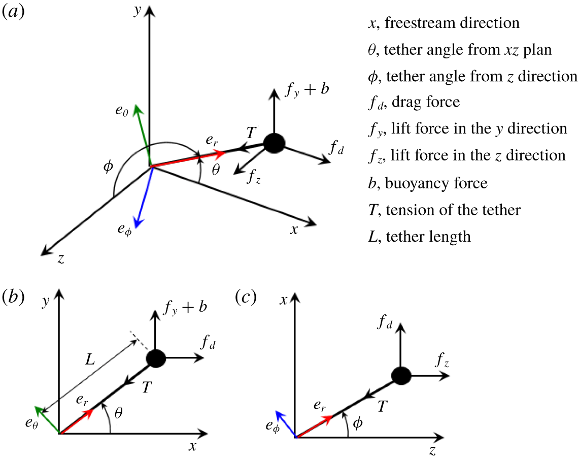
The set-up used for this computational study is simply a tethered sphere in a uniform flow field. The tether was assumed to be massless. This is compatible with experimental studies that chose a tether whose mass was negligible compared to the mass of the sphere (Williamson & Govardhan Reference Williamson and Govardhan1997; Govardhan & Williamson Reference Govardhan and Williamson1997, Reference Govardhan and Williamson2005). Moreover, the tether was assumed to be rigid and inextensible, i.e. there is no radial movement along the tether axis. This assumption is found to be justified, as experimentally there appeared to be very little movement in the radial direction. This assumption restricts the motion of the sphere to a spherical surface whose radius is the tether length. Moreover, with this holonomic constraint, the number of equations required to describe the sphere dynamics reduces to two, even though the sphere has three degrees of freedom. Moreover, the tethered sphere undergoes pure rotation around the base point of the tether. Therefore, a three-dimensional (3-D) rotation group SO(3) can also be used to obtain the equations of motion of the sphere. However, for simplicity, Newtonian mechanics principles were used here as described below.
Schematic of the tethered sphere. Two coordinate systems were used to model the system: Cartesian coordinates  $\langle i,j,k\rangle$, and spherical coordinates
 $\langle e_{r},e_{\unicode[STIX]{x1D703}},e_{\unicode[STIX]{x1D719}}\rangle$. Panel (a) shows an isometric view while (b) and (c) show the views in the
 $x$–
 $y$ and
 $z$–
 $x$ planes, respectively.

Figure 1 shows a schematic of the system. To derive the equations of motion of the sphere, a spherical coordinate system was employed with unit vectors  $\boldsymbol{e}_{r}$,
 $\boldsymbol{e}_{\unicode[STIX]{x1D703}}$ and
 $\boldsymbol{e}_{\unicode[STIX]{x1D719}}$ as shown in the figure. However, the Navier–Stokes equations were derived with a Cartesian coordinate system with unit vectors
 $\boldsymbol{i}$,
 $\boldsymbol{j}$ and
 $\boldsymbol{k}$ in the
 $x$,
 $y$ and
 $z$ directions, respectively. The mapping between these two coordinate systems is bijective and can be elaborated with parameters
 $\unicode[STIX]{x1D703}\in [0,2\unicode[STIX]{x03C0})$ and
 $\unicode[STIX]{x1D719}\in [0,\unicode[STIX]{x03C0}]$ as
 $$\begin{eqnarray}\displaystyle & \displaystyle M:\quad \left(\begin{array}{@{}c@{}}\boldsymbol{e}_{r}\\ \boldsymbol{ e}_{\unicode[STIX]{x1D703}}\\ \boldsymbol{ e}_{\unicode[STIX]{x1D719}}\end{array}\right)=\left(\begin{array}{@{}ccc@{}}\cos \unicode[STIX]{x1D703}\sin \unicode[STIX]{x1D719} & \sin \unicode[STIX]{x1D703}\sin \unicode[STIX]{x1D719} & \cos \unicode[STIX]{x1D719}\\ -\sin \unicode[STIX]{x1D703} & \cos \unicode[STIX]{x1D703} & 0\\ \cos \unicode[STIX]{x1D703}\cos \unicode[STIX]{x1D719} & \sin \unicode[STIX]{x1D703}\cos \unicode[STIX]{x1D719} & -\sin \unicode[STIX]{x1D719}\end{array}\right)\left(\begin{array}{@{}c@{}}\boldsymbol{i}\\ \boldsymbol{j}\\ \boldsymbol{k}\end{array}\right), & \displaystyle\end{eqnarray}$$
 $$\begin{eqnarray}\displaystyle & \displaystyle M^{-1}:\quad \left(\begin{array}{@{}c@{}}\boldsymbol{i}\\ \boldsymbol{j}\\ \boldsymbol{k}\end{array}\right)=\left(\begin{array}{@{}ccc@{}}\cos \unicode[STIX]{x1D703}\sin \unicode[STIX]{x1D719} & -\sin \unicode[STIX]{x1D703} & \cos \unicode[STIX]{x1D703}\cos \unicode[STIX]{x1D719}\\ \sin \unicode[STIX]{x1D703}\sin \unicode[STIX]{x1D719} & \cos \unicode[STIX]{x1D703} & \sin \unicode[STIX]{x1D703}\cos \unicode[STIX]{x1D719}\\ \cos \unicode[STIX]{x1D719} & 0 & -\sin \unicode[STIX]{x1D719}\end{array}\right)\left(\begin{array}{@{}c@{}}\boldsymbol{e}_{r}\\ \boldsymbol{ e}_{\unicode[STIX]{x1D703}}\\ \boldsymbol{ e}_{\unicode[STIX]{x1D719}}\end{array}\right). & \displaystyle\end{eqnarray}$$
Here  $\unicode[STIX]{x1D703}$ is the angle of the tether to the
 $xz$ plane and
 $\unicode[STIX]{x1D719}$ is the angle of the tether to the
 $z$ direction. In spherical coordinates, the position of the sphere,
 $\boldsymbol{r}_{s}$, can be expressed as
 $\boldsymbol{r}_{s}=L\,\boldsymbol{e}_{r}$, where
 $L$ is the length from the bottom of the tether to the centre of the sphere. Then, the velocity,
 $\boldsymbol{v}_{s}$, and the acceleration,
 $\boldsymbol{a}_{s}$, of the sphere can be obtained by differentiating the position and the velocity of the sphere with respect to time as given in equations (2.3) and (2.4), respectively:
 $$\begin{eqnarray}\displaystyle & \displaystyle \boldsymbol{v}_{s}=L(\dot{\unicode[STIX]{x1D703}}\sin \unicode[STIX]{x1D719}\,\boldsymbol{e}_{\unicode[STIX]{x1D703}}+\dot{\unicode[STIX]{x1D719}}\,\boldsymbol{e}_{\unicode[STIX]{x1D719}}), & \displaystyle\end{eqnarray}$$
 $$\begin{eqnarray}\displaystyle & \displaystyle \boldsymbol{a}_{s}=L(-(\dot{\unicode[STIX]{x1D703}}^{2}\sin ^{2}\unicode[STIX]{x1D719}+\dot{\unicode[STIX]{x1D719}}^{2})\boldsymbol{e}_{r}+(\ddot{\unicode[STIX]{x1D703}}\sin \unicode[STIX]{x1D719}+2\dot{\unicode[STIX]{x1D703}}\dot{\unicode[STIX]{x1D719}}\cos \unicode[STIX]{x1D719})\boldsymbol{e}_{\unicode[STIX]{x1D703}}+(-\dot{\unicode[STIX]{x1D703}}^{2}\sin \unicode[STIX]{x1D719}\cos \unicode[STIX]{x1D719}+\ddot{\unicode[STIX]{x1D719}})\boldsymbol{e}_{\unicode[STIX]{x1D719}}).\qquad & \displaystyle\end{eqnarray}$$
Forces acting on the sphere are of three types: a structural force  $T$ (the tension in the tether); a buoyancy force,
 $b$; and the fluid forces
 $f_{d}$,
 $f_{y}$ and
 $f_{z}$, which denote the components in the streamwise (
 $x$), lateral (
 $y$) and transverse (
 $z$) directions, respectively (see figure 1). In spherical coordinates, the summation of all forces can be written as
 $$\begin{eqnarray}\displaystyle \sum \boldsymbol{F} & = & \displaystyle (f_{d}\cos \unicode[STIX]{x1D703}\sin \unicode[STIX]{x1D719}+(f_{y}+b)\sin \unicode[STIX]{x1D703}\sin \unicode[STIX]{x1D719}+f_{z}\cos \unicode[STIX]{x1D719}-T)\boldsymbol{e}_{r}\nonumber\\ \displaystyle & & \displaystyle -\,(f_{d}\sin \unicode[STIX]{x1D703}-(f_{y}+b)\cos \unicode[STIX]{x1D703})\boldsymbol{e}_{\unicode[STIX]{x1D703}}\nonumber\\ \displaystyle & & \displaystyle +\,(f_{d}\cos \unicode[STIX]{x1D703}\cos \unicode[STIX]{x1D719}+(f_{y}+b)\sin \unicode[STIX]{x1D703}\cos \unicode[STIX]{x1D719}-f_{z}\sin \unicode[STIX]{x1D719})\boldsymbol{e}_{\unicode[STIX]{x1D719}}.\end{eqnarray}$$
Once the sphere acceleration and forces acting on it are known, the equations of motion can be easily obtained by the angular momentum balance, that is,  $I\dot{\unicode[STIX]{x1D74E}}=\sum \boldsymbol{r}\times \boldsymbol{F}$, where
 $I=m(D^{2}/10+L^{2})$ is the inertia of the sphere at the base of the tether,
 $\dot{\unicode[STIX]{x1D74E}}=\boldsymbol{a}/L$ is the angular acceleration of the sphere, and
 $m$ and
 $D$ are the mass and diameter of the sphere, respectively. The component equations are
 $$\begin{eqnarray}m(D^{2}/10+L^{2})(\ddot{\unicode[STIX]{x1D703}}\sin \unicode[STIX]{x1D719}+2\dot{\unicode[STIX]{x1D703}}\dot{\unicode[STIX]{x1D719}}\cos \unicode[STIX]{x1D719})=-L(f_{d}\sin \unicode[STIX]{x1D703}-(f_{y}+b)\cos \unicode[STIX]{x1D703}),\end{eqnarray}$$
 $$\begin{eqnarray}\displaystyle & & \displaystyle m(D^{2}/10+L^{2})(\ddot{\unicode[STIX]{x1D719}}-\dot{\unicode[STIX]{x1D703}}^{2}\sin \unicode[STIX]{x1D719}\cos \unicode[STIX]{x1D719})\nonumber\\ \displaystyle & & \displaystyle \quad =L(f_{d}\cos \unicode[STIX]{x1D703}\cos \unicode[STIX]{x1D719}+(f_{y}+b)\sin \unicode[STIX]{x1D703}\cos \unicode[STIX]{x1D719}-f_{z}\sin \unicode[STIX]{x1D719}).\end{eqnarray}$$
The above two dynamics equations can be converted into matrix form by rearranging the terms as
 $$\begin{eqnarray}\displaystyle \left(\begin{array}{@{}c@{}}\ddot{\unicode[STIX]{x1D703}}\\ \ddot{\unicode[STIX]{x1D719}}\\ 0\end{array}\right) & = & \displaystyle \frac{L}{m\left(\displaystyle {\textstyle \frac{1}{10}}D^{2}+L^{2}\right)}\left(\begin{array}{@{}ccc@{}}-\sin \unicode[STIX]{x1D703}/\sin \unicode[STIX]{x1D719} & \cos \unicode[STIX]{x1D703}/\sin \unicode[STIX]{x1D719} & 0\\ \cos \unicode[STIX]{x1D703}\cos \unicode[STIX]{x1D719} & \sin \unicode[STIX]{x1D703}\cos \unicode[STIX]{x1D719} & -\sin \unicode[STIX]{x1D719}\\ 0 & 0 & 0\end{array}\right)\left(\begin{array}{@{}c@{}}f_{d}\\ f_{y}+b\\ f_{z}\end{array}\right)\nonumber\\ \displaystyle & & \displaystyle +\,\left(\begin{array}{@{}c@{}}-2\dot{\unicode[STIX]{x1D703}}\dot{\unicode[STIX]{x1D719}}\cot \unicode[STIX]{x1D719}\\ \dot{\unicode[STIX]{x1D703}}^{2}\sin \unicode[STIX]{x1D719}\cos \unicode[STIX]{x1D719}\\ 0\end{array}\right).\end{eqnarray}$$
At this point, it is important to note that there is a singularity associated with  $\unicode[STIX]{x1D719}=0$. However, it is not a problem for the current simulations, since
 $\unicode[STIX]{x1D719}$ can never be zero because the buoyancy force is much higher than the fluid forces and, therefore, the tether can never be aligned to the transverse direction (
 $z$ direction).
The Newtonian fluid is assumed incompressible and viscous, and modelled in a Cartesian coordinate system whose origin is the centre of the sphere. This is a non-inertial reference frame, since the sphere is allowed to move according to the forces applied on it. Therefore, the acceleration of the frame should be included in the momentum equation. The acceleration of the frame is obviously the acceleration of the sphere,  $\boldsymbol{a}_{s}$, given in equation (2.4). However, since this equation is in spherical coordinates, it is necessary to first convert it into Cartesian coordinates, which can be easily done by the mapping,
 $M$, given in equation (2.1). Letting
 $\boldsymbol{a}_{c}$ be the acceleration of the frame once it is converted into Cartesian coordinates, then
 $$\begin{eqnarray}\displaystyle \boldsymbol{a}_{c}=M(\boldsymbol{a}_{s}). & & \displaystyle\end{eqnarray}$$
Finally, the coupled fluid–solid system can be described by the Navier–Stokes equations given in (2.10) and (2.11) and the sphere motion equations given in (2.8) together with equations (2.1), (2.4) and (2.9):
 $$\begin{eqnarray}\displaystyle & \displaystyle \frac{\unicode[STIX]{x2202}\boldsymbol{u}}{\unicode[STIX]{x2202}t}=-(\boldsymbol{u}\boldsymbol{\cdot }\unicode[STIX]{x1D735})\boldsymbol{u}-\frac{1}{\unicode[STIX]{x1D70C}}\unicode[STIX]{x1D735}p+\unicode[STIX]{x1D735}\boldsymbol{\cdot }\unicode[STIX]{x1D708}\unicode[STIX]{x1D735}\boldsymbol{u}-\boldsymbol{a}_{c}, & \displaystyle\end{eqnarray}$$
 $$\begin{eqnarray}\displaystyle & \displaystyle \unicode[STIX]{x1D735}\boldsymbol{\cdot }\boldsymbol{u}=0, & \displaystyle\end{eqnarray}$$
where  $\boldsymbol{u}=\boldsymbol{u}(x,y,z,t)$ is the velocity vector field,
 $p$ is the scalar pressure field,
 $\unicode[STIX]{x1D70C}$ is the fluid density and
 $\unicode[STIX]{x1D708}$ is the kinematic viscosity of the fluid.
2.2 FSI solver for a tethered sphere
A new fully coupled solver (named ‘tetheredVivIcoFoam’) was developed, based on the in-built ‘icoFoam’ solver for laminar flows, to solve the coupled fluid–solid system defined by equations (2.8)–(2.11) for a tethered sphere.
The icoFoam solver was developed based on the pressure-implicit with splitting of operators (PISO) algorithm introduced by Issa (Reference Issa1986). At a given time step, this algorithm initiates by setting up the boundary conditions. In the predictor iteration, the discretized momentum equations are solved for an intermediate velocity field, based on the pressure field and the flux calculated in the previous time step. Then, in a corrector iteration, first, the mass fluxes of the cell faces are computed, and then the pressure equation (which satisfies the continuity equation) is solved for the pressure. Next, the mass fluxes on the cell faces and the velocities are corrected based on the new pressure field. Finally, the boundary conditions are updated. Issa (Reference Issa1986) showed that two corrector iterations are sufficient to achieve second-order accuracy, as the whole PISO algorithm is second-order-accurate.
Similar to the solver we previously developed for the FIV of an elastically mounted solid body (Rajamuni et al. Reference Rajamuni, Thompson and Hourigan2018a, § 2.2), the tetheredVivIcoFoam solver employs a predictor–corrector iterative method. The solid motion was first predicted explicitly in the predictor iteration and then corrected as necessary with several corrector iterations. Once the solid motion is obtained (from the predictor or a corrector iteration), the Navier–Stokes equations were solved using the PISO algorithm by treating the acceleration of the frame as a source term. This iterative process for the  $(n+1)$th time step can be elaborated as follows:
The predictor iteration. Initially, the angular accelerations of the sphere,  $(\ddot{\unicode[STIX]{x1D703}}~\ddot{\unicode[STIX]{x1D719}})^{\text{T}}$, are predicted explicitly using a third-order polynomial interpolation by
 $$\begin{eqnarray}\displaystyle \left(\begin{array}{@{}c@{}}\ddot{\unicode[STIX]{x1D703}}\\ \ddot{\unicode[STIX]{x1D719}}\end{array}\right)^{(n+1)}=3\left(\begin{array}{@{}c@{}}\ddot{\unicode[STIX]{x1D703}}\\ \ddot{\unicode[STIX]{x1D719}}\end{array}\right)^{(n)}-3\left(\begin{array}{@{}c@{}}\ddot{\unicode[STIX]{x1D703}}\\ \ddot{\unicode[STIX]{x1D719}}\end{array}\right)^{(n-1)}+\left(\begin{array}{@{}c@{}}\ddot{\unicode[STIX]{x1D703}}\\ \ddot{\unicode[STIX]{x1D719}}\end{array}\right)^{(n-2)}. & & \displaystyle\end{eqnarray}$$
Then, the angular velocities,  $(\dot{\unicode[STIX]{x1D703}}~\dot{\unicode[STIX]{x1D719}})^{\text{T}}$, and tether angles,
 $(\unicode[STIX]{x1D703}~\unicode[STIX]{x1D719})^{\text{T}}$, are estimated using a third-order Adams–Moulton method by integrating the angular accelerations and angular velocities to obtain
 $$\begin{eqnarray}\displaystyle \left(\begin{array}{@{}c@{}}\dot{\unicode[STIX]{x1D703}}\\ \dot{\unicode[STIX]{x1D719}}\end{array}\right)^{(n+1)}=\left(\begin{array}{@{}c@{}}\dot{\unicode[STIX]{x1D703}}\\ \dot{\unicode[STIX]{x1D719}}\end{array}\right)^{(n)}+\frac{\unicode[STIX]{x1D6FF}t}{12}\left(\begin{array}{@{}c@{}}5\left(\begin{array}{@{}c@{}}\ddot{\unicode[STIX]{x1D703}}\\ \ddot{\unicode[STIX]{x1D719}}\end{array}\right)^{(n+1)}+8\left(\begin{array}{@{}c@{}}\ddot{\unicode[STIX]{x1D703}}\\ \ddot{\unicode[STIX]{x1D719}}\end{array}\right)^{(n)}-\left(\begin{array}{@{}c@{}}\ddot{\unicode[STIX]{x1D703}}\\ \ddot{\unicode[STIX]{x1D719}}\end{array}\right)^{(n-1)}\end{array}\right) & & \displaystyle\end{eqnarray}$$
and
 $$\begin{eqnarray}\displaystyle \left(\begin{array}{@{}c@{}}\unicode[STIX]{x1D703}\\ \unicode[STIX]{x1D719}\end{array}\right)^{(n+1)}=\left(\begin{array}{@{}c@{}}\unicode[STIX]{x1D703}\\ \unicode[STIX]{x1D719}\end{array}\right)^{(n)}+\frac{\unicode[STIX]{x1D6FF}t}{12}\left(\begin{array}{@{}c@{}}5\left(\begin{array}{@{}c@{}}\dot{\unicode[STIX]{x1D703}}\\ \dot{\unicode[STIX]{x1D719}}\end{array}\right)^{(n+1)}+8\left(\begin{array}{@{}c@{}}\dot{\unicode[STIX]{x1D703}}\\ \dot{\unicode[STIX]{x1D719}}\end{array}\right)^{(n)}-\left(\begin{array}{@{}c@{}}\dot{\unicode[STIX]{x1D703}}\\ \dot{\unicode[STIX]{x1D719}}\end{array}\right)^{(n-1)}\end{array}\right), & & \displaystyle\end{eqnarray}$$
respectively. Then, the acceleration of the sphere,  $\boldsymbol{a}_{s}^{(n+1)}$, is obtained by equation (2.4) and converted into Cartesian coordinates,
 $\boldsymbol{a}_{c}^{(n+1)}$, using the mapping given in equation (2.1). At the end of the predictor step, the Navier–Stokes equations given in (2.10) and (2.11) are solved with the predicted
 $\boldsymbol{a}_{c}^{(n+1)}$ and the forces exerted on the sphere,
 $(f_{d}\,~f_{y}\,~f_{z})^{(n+1)}$, are calculated.
A corrector iteration. Initially, the angular accelerations of the sphere,  $(\ddot{\unicode[STIX]{x1D703}}~\ddot{\unicode[STIX]{x1D719}})^{\text{T}}$, are corrected by equation (2.8) with the values obtained for
 $\unicode[STIX]{x1D703}$,
 $\unicode[STIX]{x1D719}$,
 $\dot{\unicode[STIX]{x1D703}}$,
 $\dot{\unicode[STIX]{x1D719}}$,
 $f_{d}$,
 $f_{y}$ and
 $f_{z}$ at the predictor iteration (or at the last corrector iteration). Then, the corrected angular accelerations are relaxed to improve the convergence characteristics by
 $$\begin{eqnarray}\displaystyle \left(\begin{array}{@{}c@{}}\ddot{\unicode[STIX]{x1D703}}\\ \ddot{\unicode[STIX]{x1D719}}\end{array}\right)^{(n+1)\prime }=\left(\begin{array}{@{}c@{}}\ddot{\unicode[STIX]{x1D703}}\\ \ddot{\unicode[STIX]{x1D719}}\end{array}\right)^{(n+1)\ast }+\unicode[STIX]{x1D6FE}\left(\begin{array}{@{}c@{}}\left(\begin{array}{@{}c@{}}\ddot{\unicode[STIX]{x1D703}}\\ \ddot{\unicode[STIX]{x1D719}}\end{array}\right)^{(n+1)\ast \ast }-\left(\begin{array}{@{}c@{}}\ddot{\unicode[STIX]{x1D703}}\\ \ddot{\unicode[STIX]{x1D719}}\end{array}\right)^{(n+1)\ast }\end{array}\right), & & \displaystyle\end{eqnarray}$$
where  $\unicode[STIX]{x1D6FE}$ is the relaxation parameter, and
 $\ast$ and
 $\ast \ast$ represent the angular accelerations calculated in the previous and the current iterations, respectively. The method becomes unstable, especially for small-mass-ratio spheres in the absence of any relaxation. The convergence of the method can be improved by the choice of
 $\unicode[STIX]{x1D6FE}$, depending on the parameter combination. In the literature, Le Tallec & Mouro (Reference Le Tallec and Mouro2001), Causin, Gerbeau & Nobile (Reference Causin, Gerbeau and Nobile2005) and Borazjani, Ge & Sotiropoulos (Reference Borazjani, Ge and Sotiropoulos2008) have also used under-relaxation schemes to improve the stability of their FSI algorithms. Once the angular accelerations are corrected and relaxed, the angular velocities and tether angles are calculated, similar to the predictor step. With these newly calculated values, the sphere acceleration (in Cartesian coordinates) is calculated and the Navier–Stokes equations are solved. Finally, the fluid forces exerted on the sphere are calculated to use in the next corrector iteration. This iterative process is terminated once the magnitude of the fluid forces and sphere angular accelerations are converged within the given tolerance limit,
 $\unicode[STIX]{x1D716}=0.001$. This value was chosen for simulations since it was found that further decreasing
 $\unicode[STIX]{x1D716}$ does not increase the accuracy of the solution.
The temporal accuracy of the overall FSI solver is second-order, although the solution process for the solid motion is third-order-accurate. This is because the PISO algorithm itself is of second-order accuracy. As described in the previous section, the fluid flow is modelled in the moving frame that is attached to the centre of the sphere. This motion is acknowledged through the outer domain velocity boundary conditions (except the outlet boundary). In this study, all the outer boundaries, except the outlet, where a pressure condition is enforced, have velocity prescribed on them. Once the predictor–corrector iterative process is completed, the velocity boundary conditions are updated according to the sphere velocity,  $\boldsymbol{v}_{c}=M(\boldsymbol{v}_{s})$.
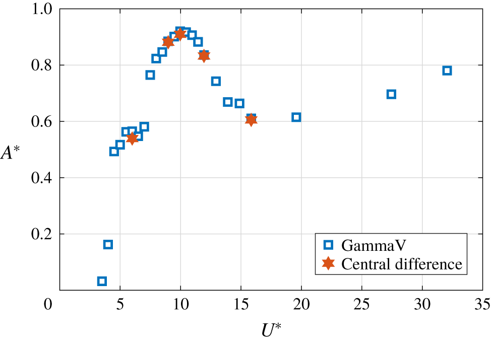
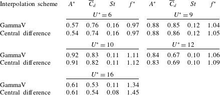
OpenFOAM is a cell-centred finite-volume code that offers a number of different choices for the temporal and spatial discretization of the different terms in the Navier–Stokes equations. The choices made for the current simulations were as follows. The second-order backward scheme was used to integrate forwards in time. This uses a stencil based on the solution at three time levels to achieve the desired second-order accuracy (see Jasak Reference Jasak1995). Both the pressure and diffusion terms were discretized using second-order centred approximations. The convection terms were treated using the GammaV scheme with  $\unicode[STIX]{x1D6FD}=0.5$. This scheme is based on the normalized variable diagram (NVD) approach originally introduced by (Leonard Reference Leonard1991), which is very similar to the total variation diminishing approach. The GammaV variation (Jasak, Weller & Gosman Reference Jasak, Weller and Gosman1999) employs the central-difference approximation limited by the upwind approximation to prevent unphysical overshoots of the evolving solution near sharp changes in the solution, otherwise characteristic of the pure central-difference scheme. Tests show that, on a standard convection problem of advection of a step change (e.g. see figure 15 of Jasak et al. (Reference Jasak, Weller and Gosman1999)), the step variation is resolved almost as well as the second-order central-difference discretization, but avoiding the artificial diffusion of the upwind scheme. Naturally, it provides a pure second-order solution as the grid is refined, and indeed convergence (grid independence) was verified for this study through standard resolution studies described below. However, given that the advection schemes such as the GammaV scheme are not normally used for incompressible flow problems, further substantiation that the predictions do not depend on this choice of discretization approach is provided in the appendix. In particular, it is shown that the choice of the standard purely second-order central-difference scheme for the advection terms gives essentially the same predictions of the amplitude response curve (and shedding modes) at the highest Reynolds number studied (
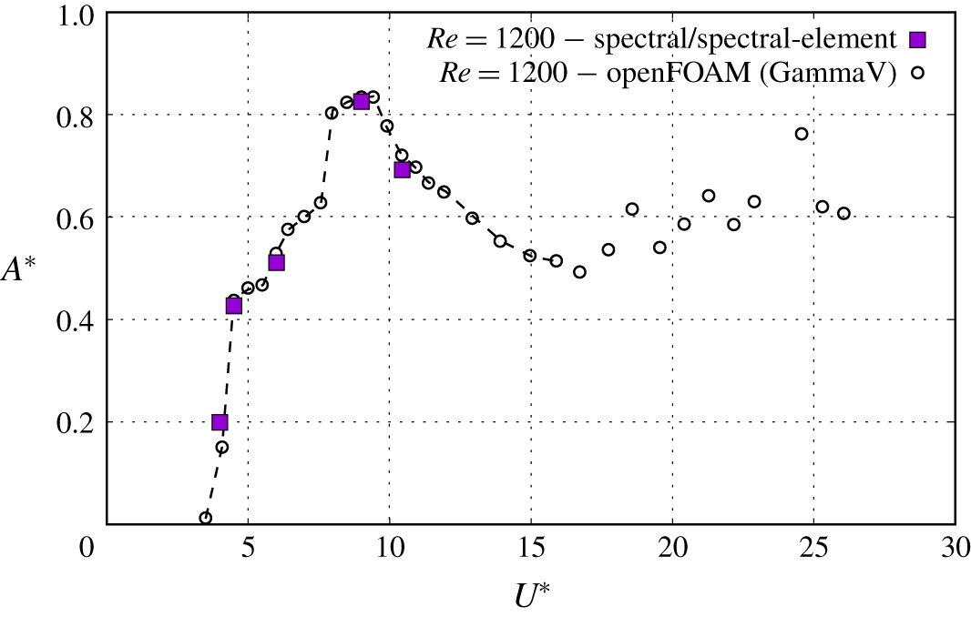
 $Re=2000$). In addition, an independent check using a spectral/spectral-element code also predicts the same response curve as the GammaV scheme for the intermediate-Reynolds-number case (
 $Re=1200$). These additional studies provide further support that the predictions presented in this paper and implementation of the model in the code are reliable.
For the flow solver to be stable, the time step should be chosen such that it satisfies the Courant condition,  $u\unicode[STIX]{x0394}t/\unicode[STIX]{x0394}x<1$, everywhere. The time step used for all of the simulations presented in this paper was
 $0.005U/D$. This is found to be sufficient to ensure the Courant number is less than unity over the entire domain.
2.3 Dynamic mode decomposition
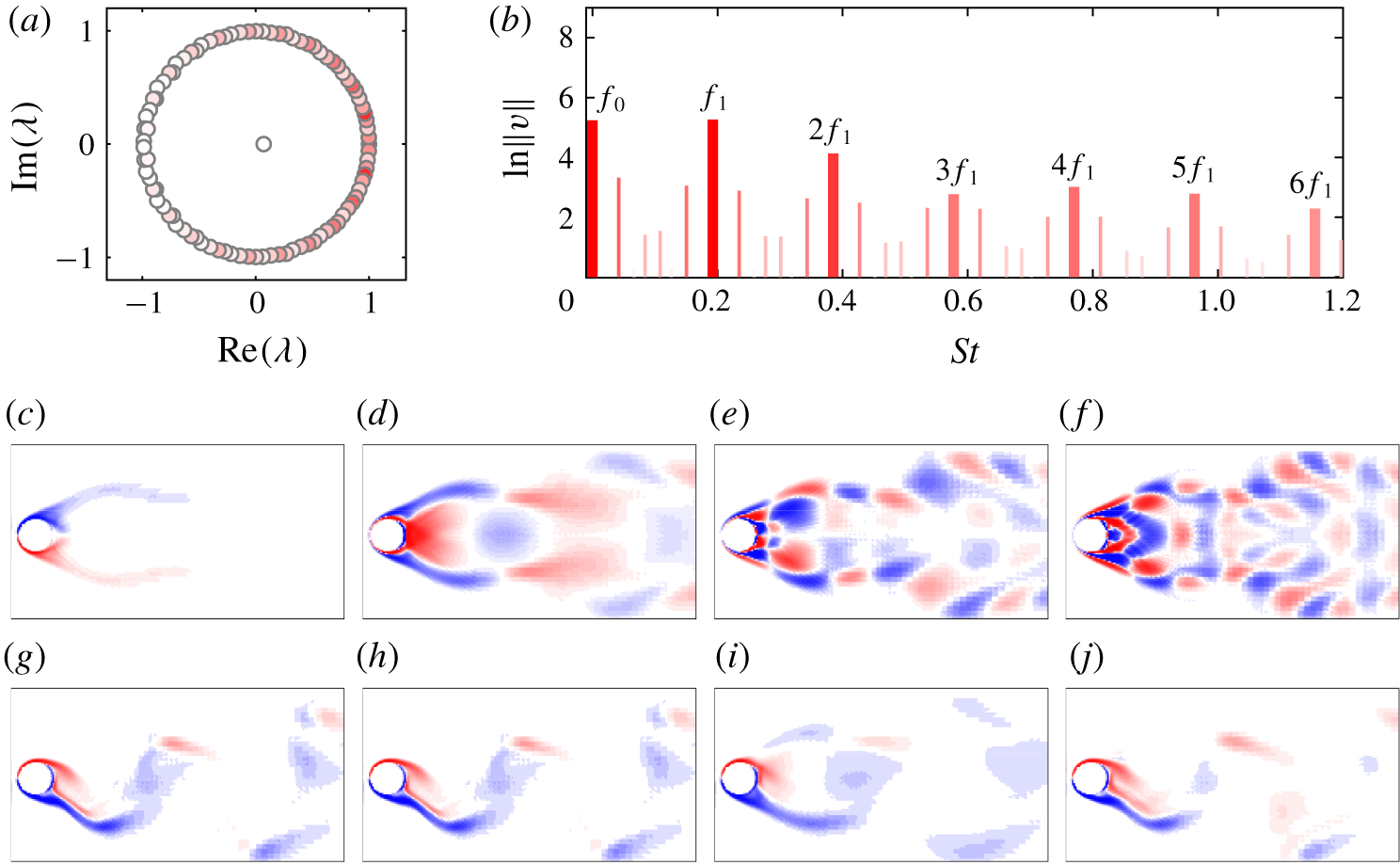
Dynamic mode decomposition (DMD) is also used as part of the analysis to characterize the wake behind the sphere. DMD is a numerical procedure introduced by Schmid & Sesterhenn (Reference Schmid and Sesterhenn2008) for extracting the dynamic periodic features of a flow. This method involves spectral analysis of the Koopman operator. For a given sequence of time-resolved flow field measurements, in this the case consisting of a set of velocity fields at fixed time increments, DMD computes a set of approximations to the Koopman modes, also called Ritz vectors, with associated eigenvalues, called Ritz values. Ritz vectors are the eigenfunctions of the Koopman operator, each of which is associated with a fixed oscillation frequency specified by the argument of the associated eigenvalue. A Koopman mode may grow or decay exponentially in time, according to the magnitude of the corresponding eigenvalue. In particular, this analysis is useful to extract the dominant frequencies belonging to the sequence of fields and the corresponding periodic spatially varying modes, which may be localized in different regions of space. The approach used here closely follows that of Rowley et al. (Reference Rowley, Mezić, Bagheri, Schlatter and Henningson2009) and Schmid (Reference Schmid2010, Reference Schmid2011), so only a very brief outline is given here.
Let  $\boldsymbol{x}_{1},\boldsymbol{x}_{2},\ldots ,\boldsymbol{x}_{m}$ represent a set of column vectors of the field data (e.g. velocity field), collected at equal time intervals
 $\unicode[STIX]{x1D6FF}t$. Following the Krylov technique, in particular, the Arnoldi approach,
 $\boldsymbol{x}_{m}$ can be expressed as a linearly independent combination of
 $\boldsymbol{x}_{1},\boldsymbol{x}_{2},\ldots ,\boldsymbol{x}_{m-1}$, leading to the following matrix equation:
 $$\begin{eqnarray}\left(\begin{array}{@{}cccc@{}}\boldsymbol{x}_{\mathbf{2}}~| & \boldsymbol{x}_{\mathbf{3}}~| & \ldots ~| & \boldsymbol{x}_{\boldsymbol{m}}\end{array}\right)=\left(\begin{array}{@{}cccc@{}}\boldsymbol{x}_{\mathbf{1}}~| & \boldsymbol{x}_{\mathbf{2}}~| & \ldots ~| & \boldsymbol{x}_{\boldsymbol{m}-\mathbf{1}}\end{array}\right)\left(\begin{array}{@{}ccccc@{}}0 & 0 & \ldots & 0 & c_{1}\\ 1 & 0 & \ldots & 0 & c_{2}\\ 0 & 1 & \ldots & 0 & c_{3}\\ \vdots & \vdots & \ddots & \vdots & \vdots \\ 0 & 0 & \ldots & 1 & c_{m-1}\end{array}\right)\equiv \boldsymbol{K}\unicode[STIX]{x1D63E}.\end{eqnarray}$$
The matrix  $\unicode[STIX]{x1D63E}$ is called the companion matrix, which is the equivalent low-dimensional representation of the field data. Since the vectors
 $\boldsymbol{x}_{0},\ldots ,\boldsymbol{x}_{m}$ are known, the coefficients,
 $c_{1},\ldots ,c_{m-1}$ can be easily obtained by the
 $QR$ factorization or singular value decomposition. Let
 $\boldsymbol{z}_{i}$ and
 $\unicode[STIX]{x1D706}_{i}$ be the
 $i$th eigenvector and eigenvalue of
 $\unicode[STIX]{x1D63E}$, respectively. Then, the Koopman modes (Ritz vectors) of the dataset can be obtained by
 $$\begin{eqnarray}\boldsymbol{v}_{i}=\boldsymbol{K}\boldsymbol{z}_{i},\end{eqnarray}$$
and the Ritz values are directly the eigenvalues of the companion matrix. Note that both the Ritz vectors and values consist of complex conjugate pairs.
The field at any discrete time  $t_{k}$ can be reconstructed using the Ritz vectors and values. However, the Ritz vectors should be obtained from the properly rescaled eigenvalues for the reconstructions. Let
 $\hat{\boldsymbol{z}}_{i}=\unicode[STIX]{x1D6FD}_{i}\boldsymbol{z}_{i}$ be the scaled version of
 $\boldsymbol{z}_{i}$ using the
 $i$th element of the vector,
 $\unicode[STIX]{x1D737}=\unicode[STIX]{x1D655}^{-1}\boldsymbol{e}_{1}$, where
 $\unicode[STIX]{x1D655}=[\boldsymbol{z}_{1}~\boldsymbol{z}_{2}~\ldots ~\boldsymbol{z}_{m-1}]$ and
 $\boldsymbol{e}_{1}=(1~0~\ldots ~0)^{\text{T}}$. If
 $\hat{\boldsymbol{v}}_{i}=\unicode[STIX]{x1D646}\hat{\boldsymbol{z}}_{i}$ is the scaled Ritz vector, then the field at any discrete time
 $t_{k}$ can be reconstructed by
 $$\begin{eqnarray}\boldsymbol{x}_{k}=\mathop{\sum }_{i=1}^{m-1}\unicode[STIX]{x1D706}_{i}^{k}\hat{\boldsymbol{v}}_{i}.\end{eqnarray}$$
If the sequence of fields is strictly periodic, so that  $\boldsymbol{x}_{m}=\boldsymbol{x}_{1}$, then the above expansion is equivalent to a Fourier decomposition.
2.4 The natural frequency
The reduced velocity,  $U^{\ast }=U/(f_{n}D)$, is identified as a suitable parameter for FIV problems as it is a function of the system’s natural frequency. In experiments, a range of reduced velocity is obtained by increasing the flow velocity,
 $U$. Since the Reynolds number is also a function of the flow velocity, it is impracticable to increase the reduced velocity by fixing the Reynolds number. This is an undesirable side-effect that appears in experiments. However, when performing simulations, it is desirable to fixed the Reynolds number at a suitable value. This limits the number of varying parameters for each set of simulations. Moreover, if the Reynolds number is increased, then the laminar flow transitions to turbulence by introducing small scales of motion. To accurately predict these small scales, a finer mesh density is required. However, this increases the computational cost considerably.
Williamson & Govardhan (Reference Williamson and Govardhan1997) obtained an expression for the non-dimensional natural frequency of the tethered sphere system as
 $$\begin{eqnarray}\displaystyle S_{n}\approx \left(\frac{1}{2\unicode[STIX]{x03C0}}\right)\frac{1}{Fr\sqrt{l^{\ast }}}\,\sqrt{\frac{1-m^{\ast }}{C_{a}+m^{\ast }}}, & & \displaystyle\end{eqnarray}$$
where  $C_{a}$ is the added-mass coefficient (
 $0.5$ for a sphere). The mass ratio,
 $m^{\ast }$, and the tether length ratio,
 $l^{\ast }=L/D$, are desired to be kept constant for a particular set of simulations. Therefore, it is possible to obtain a range of natural frequencies (reciprocal of the reduced velocity) by varying the Froude number,
 $Fr$, numerically. The Froude number is a non-dimensional number defined as the ratio of the flow inertia to the gravitational force (
 $Fr=U/\sqrt{gD}$, where
 $g$ is the gravitational force). Furthermore, it is conceivably possible to investigate numerically as
 $U^{\ast }\rightarrow \infty$, whereas the reduced velocity range is limited experimentally to the flow velocity accessible in the flow facility. For the present study, three sets of simulations were performed by fixing the Reynolds number at
 $Re=500$,
 $1200$ and
 $2000$. Studying the cases for the Reynolds numbers
 $Re=1200$ and
 $2000$, which are closer to the experimental studies of Williamson & Govardhan (Reference Williamson and Govardhan1997), Govardhan & Williamson (Reference Govardhan and Williamson1997, Reference Govardhan and Williamson2005) and Jauvtis et al. (Reference Jauvtis, Govardhan and Williamson2001), provides additional insight into those studies, while the case of
 $Re=500$ will provide an understanding of the problem in the laminar regime.
2.5 Calculation of the reduced velocity
To obtain a range of reduced velocities, it is required to calculate the natural frequency of the tethered system accurately, which is the focus of this section.
Let  $(X,Y,Z)^{\text{T}}$ be the position of the sphere in Cartesian coordinates. Then, the equation of motion of the tethered sphere can be obtained by the linear momentum balance (see figure 1) as
 $$\begin{eqnarray}\displaystyle m\left(\begin{array}{@{}c@{}}\ddot{X}\\ \ddot{Y} \\ \ddot{Z}\end{array}\right)=\left(\begin{array}{@{}c@{}}f_{d}\\ f_{y}+b\\ f_{z}\end{array}\right)-T\left(\begin{array}{@{}c@{}}\sin \unicode[STIX]{x1D719}\cos \unicode[STIX]{x1D703}\\ \sin \unicode[STIX]{x1D719}\sin \unicode[STIX]{x1D703}\\ \cos \unicode[STIX]{x1D719}\end{array}\right). & & \displaystyle\end{eqnarray}$$
However,  $(\sin \unicode[STIX]{x1D719}\cos \unicode[STIX]{x1D703},\;\sin \unicode[STIX]{x1D719}\sin \unicode[STIX]{x1D703},\;\cos \unicode[STIX]{x1D719})^{\text{T}}$ is the unit vector along the tether,
 $\boldsymbol{e}_{r}$, and can be expressed as
 $(X,Y,Z)^{\text{T}}/L$. Hence, the equations of motion can be rearranged into
 $$\begin{eqnarray}\displaystyle m\left(\begin{array}{@{}c@{}}\ddot{X}\\ \ddot{Y} \\ \ddot{Z}\end{array}\right)-\frac{T}{L}\left(\begin{array}{@{}c@{}}X\\ Y\\ Z\end{array}\right)=\left(\begin{array}{@{}c@{}}f_{d}\\ f_{y}+b\\ f_{z}\end{array}\right). & & \displaystyle\end{eqnarray}$$
From these equations, it is clear that the natural frequency of the system is identical in all three directions and is given by
 $$\begin{eqnarray}\displaystyle f_{n}=\frac{1}{2\unicode[STIX]{x03C0}}\sqrt{\frac{T}{mL}}. & & \displaystyle\end{eqnarray}$$
This can be written in the non-dimensional form as
 $$\begin{eqnarray}\displaystyle S_{n}=\frac{\,f_{n}D}{U}=\frac{1}{2\unicode[STIX]{x03C0}}\sqrt{\frac{D^{2}T}{U^{2}mL}}. & & \displaystyle\end{eqnarray}$$
Since the sphere is assumed to have no motion in the direction of the tether, the tension of the tether can be obtained simply from the force balance as
 $$\begin{eqnarray}\displaystyle T=\sqrt{f_{d}^{2}+(f_{y}+b)^{2}+f_{z}^{2}}, & & \displaystyle\end{eqnarray}$$
assuming the centrifugal force is negligible, consistent with a large tether length ratio. With this expression for  $T$, equation (2.23) can be written in the non-dimensional form as
 $$\begin{eqnarray}\displaystyle S_{n}=\frac{1}{2\unicode[STIX]{x03C0}}\sqrt{\frac{\sqrt{C_{d}^{2}+\{C_{y}+(1-m^{\ast })\unicode[STIX]{x1D6FC}\}^{2}+C_{z}^{2}}}{(4/3)(m^{\ast }+C_{a})l^{\ast }}}, & & \displaystyle\end{eqnarray}$$
where  $\unicode[STIX]{x1D6FC}=4/(3Fr^{2})$. For a stationary sphere, the time-averaged lateral (
 $y$) and transverse (
 $z$) forces are negligible compared to the drag force. Moreover,
 $(1-m^{\ast })\unicode[STIX]{x1D6FC}$ is much greater than
 $C_{y}$ over the entire reduced velocity range investigated for the mass ratios of interest in this study (
 $m^{\ast }=0.8$ and
 $80$). Hence, (2.25) can be simplified to
 $$\begin{eqnarray}\displaystyle S_{n}\approx \frac{1}{2\unicode[STIX]{x03C0}}\sqrt{\frac{\sqrt{C_{d}^{2}+\{(1-m^{\ast })\unicode[STIX]{x1D6FC}\}^{2}}}{(4/3)(m^{\ast }+C_{a})l^{\ast }}}. & & \displaystyle\end{eqnarray}$$
The reduced velocity,  $U^{\ast }$, is defined as the inverse of the natural frequency,
 $S_{n}$, leading to
 $$\begin{eqnarray}\displaystyle U^{\ast }=2\unicode[STIX]{x03C0}\sqrt{\frac{(4/3)(m^{\ast }+C_{a})l^{\ast }}{\sqrt{C_{d}^{2}+\{(1-m^{\ast })\unicode[STIX]{x1D6FC}\}^{2}}}}. & & \displaystyle\end{eqnarray}$$
For all of the numerical results to be presented, equation (2.27) has been used to calculate the reduced velocity. A range of  $U^{\ast }$ is obtained by varying
 $\unicode[STIX]{x1D6FC}$. In experiments, since the gravitational acceleration is constant,
 $C_{d}$ is negligible compared to the buoyancy force component, and therefore
 $S_{n}$ given in (2.19) is valid. In contrast, in this numerical study, the buoyancy term is of the same order of magnitude as the drag coefficient for higher reduced velocities. Therefore, it is required to use equation (2.27) instead of equation (2.19).
3 Numerical sensitivity and validation studies
3.1 Grid and domain details
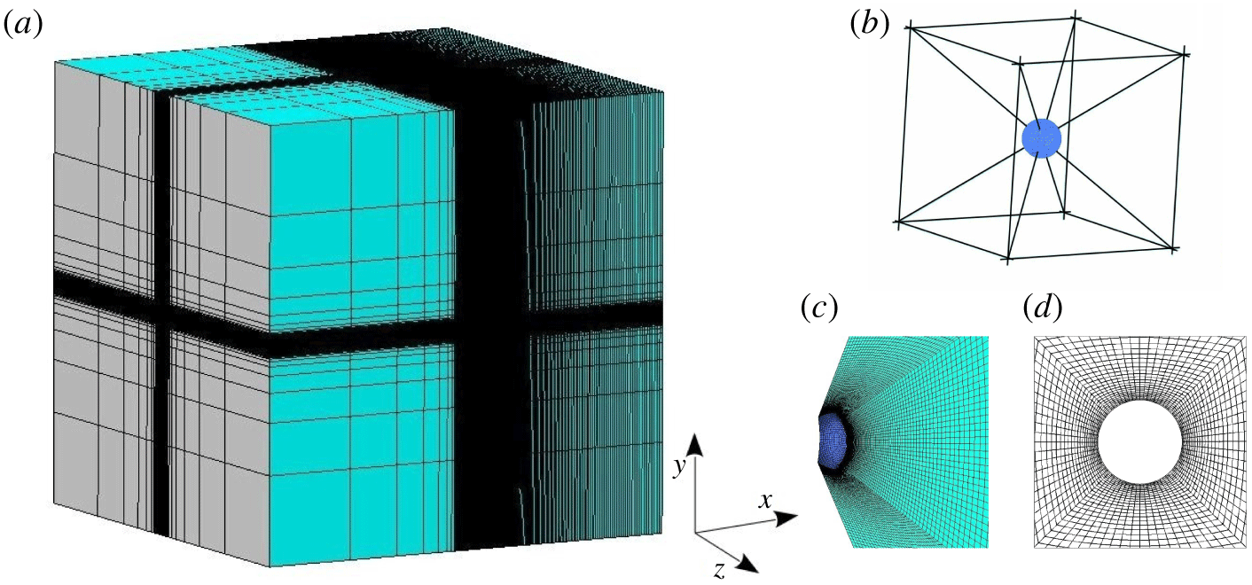
A cubical domain with a side length of  $100D$ was chosen for the fluid with the sphere at its centre. Figure 2 shows the hexahedral grid generated using Ansys-ICEM-CFD for the fluid domain. A cubic block with a side length of
 $5D$ was placed around the sphere to achieve greater resolution near the sphere (see figure 2b). This cube was first decomposed into six square frustums. The grid was concentrated towards the sphere surface by assigning exponentially distributed grid points in the radial direction of each square frustum (see figure 2c,d). Uniformly distributed grid points were assigned in the other two directions of each square frustum. A large number of grid points were assigned in the downstream direction to reasonably resolve the wake structures.
The hexahedral grid computational domain: (a) isometric view; (b) cubic block placed around the sphere, which was decomposed into six square frustums; (c) isometric view of the grid in a square frustum near the sphere surface; and (d) grid near the sphere surface in the  $x$–
 $y$ plane.

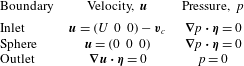
Boundary conditions, where  $U$ is the upstream velocity,
 $\boldsymbol{\unicode[STIX]{x1D702}}$ is the outward normal vector at the corresponding boundary and
 $\boldsymbol{v}_{c}$ is the velocity of the sphere motion.

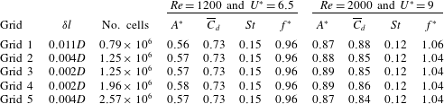
Five successively finer grids were constructed to analyse the dependence of the computed solution on the grid refinement (see the next section). The first four grids were generated by fixing the number of cells in the sphere boundary,  $N=7350$. Grid 1 contains
 $\simeq 0.79$ million cells whose cell thickness at the sphere boundary,
 $\unicode[STIX]{x1D6FF}l$, is
 $0.011D$. Grid
 $2$ was created by decreasing
 $\unicode[STIX]{x1D6FF}l$ to
 $0.004D$. This yielded
 $\simeq 1.25$ million cells, with approximately 10–16 cells within the boundary layer before flow separation. This grid is fine enough for this numerical study. However, a few more grids were generated to confirm that the solution is insensitive to further refinement of the grid. Grid
 $3$ was generated by decreasing
 $\unicode[STIX]{x1D6FF}l$ further down to
 $0.002D$, but with the same number of cells as grid
 $2$ to obtain more concentration towards the sphere boundary. Grid
 $4$ was generated by doubling the number of nodes in the radial direction of a square frustum with the same
 $\unicode[STIX]{x1D6FF}l$ as grid
 $3$. This increased the number of cells to
 $\simeq 1.96~\text{million}$. Finally, to analyse the effect of grid refinement in the tangential direction, grid
 $5$ was generated by increasing the number of cells in the sphere boundary,
 $N$, to
 $18\,150$ with
 $\unicode[STIX]{x1D6FF}l=0.004D$, which is the same
 $\unicode[STIX]{x1D6FF}l$ as grid
 $2$.
The cubical fluid domain has two types of outer boundaries, inlet and outlet. Five sides of the cube were treated as inlets and the velocity is prescribed on them. As described earlier, the motion of the frame was taken into account through these inlets by updating the frame velocity at each time step. The remaining side of the cube is the outlet with a zero pressure. The inner boundary (sphere boundary) is treated as a wall and assumed to have no-slip and no-penetration boundary conditions. The flow is assumed in the  $x$ direction; boundary conditions for pressure and velocity at each boundary are tabulated in table 1.
3.2 Validation study
The flow past a rigidly mounted sphere was investigated at  $Re=500$ and
 $1000$. The computed values for the time-averaged drag and lift coefficients,
 $\overline{C}_{d}$ and
 $\overline{C}_{l}$, respectively, and the Strouhal number,
 $St$, are listed in table 2. As the lift coefficient is negligible at
 $Re=1000$, a secondary Strouhal number is calculated instead of
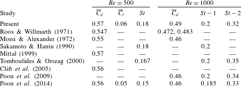
 $\overline{C}_{l}$. As can be seen, the present results closely match values calculated in other studies (Roos & Willmarth Reference Roos and Willmarth1971; Morsi & Alexander Reference Morsi and Alexander1972; Sakamoto & Haniu Reference Sakamoto and Haniu1990; Mittal Reference Mittal1999; Tomboulides & Orszag Reference Tomboulides and Orszag2000; Clift, Grace & Weber Reference Clift, Grace and Weber2005; Poon et al. Reference Poon, Iaccarino, Ooi and Giacobello2009, Reference Poon, Ooi, Giacobello, Iaccarino and Chung2014).
Comparison of computed time-averaged drag coefficient,  $\overline{C}_{d}$, time-averaged lift coefficient,
 $\overline{C_{l}}$, and Strouhal number,
 $St$, at
 $Re=500$ and
 $1000$ with other studies.

The sensitivity of the spatial resolution of the flow parameters of VIV of a tethered sphere at  $m^{\ast }=0.8$ for
 $(Re,U^{\ast })=(1200,6.5)$, representing mode I, and
 $(2000,9)$, representing mode II. Here
 $\unicode[STIX]{x1D6FF}l$ is the minimum thickness of the cells (in the radial direction) at the sphere boundary in each grid. The oscillation amplitude of the sphere,
 $A^{\ast }$, the time-mean drag,
 $\overline{C}_{d}$, Strouhal number,
 $St$, and the ratio of vortex shedding frequency to the natural frequency,
 $f^{\ast }=f/f_{n}$, are listed.

3.3 Grid-independence analysis
The sensitivity of the solution to the spatial resolution was investigated with a sphere of mass ratio  $m^{\ast }=0.8$ at
 $(Re,U^{\ast })=(1200,6.5)$ and
 $(2000,9)$. The reduced velocities of
 $6.5$ and
 $9$ were chosen to represent mode I and II states, respectively. The r.m.s. of the response amplitude,
 $A^{\ast }$, the time-averaged drag coefficient,
 $\overline{C}_{d}$, the Strouhal number,
 $St$, and the frequency ratio,
 $f^{\ast }=f/f_{n}$, were calculated with each grid, and the results are tabulated in table 3. As can be seen, the results match reasonably well with each other for all five grids at both reduced velocities, as a result of employing finer grids in each case. The percentage error difference among all of the quantities from grid
 $2$ to grid
 $5$ is at most
 $3\,\%$. Grid
 $3$ was chosen for the simulations as it is concentrated towards the sphere and better captures the boundary layers.
4 Results
4.1 FIV response of a tethered sphere
The flow past a tethered sphere of mass ratio  $m^{\ast }=0.8$ with a tether length of
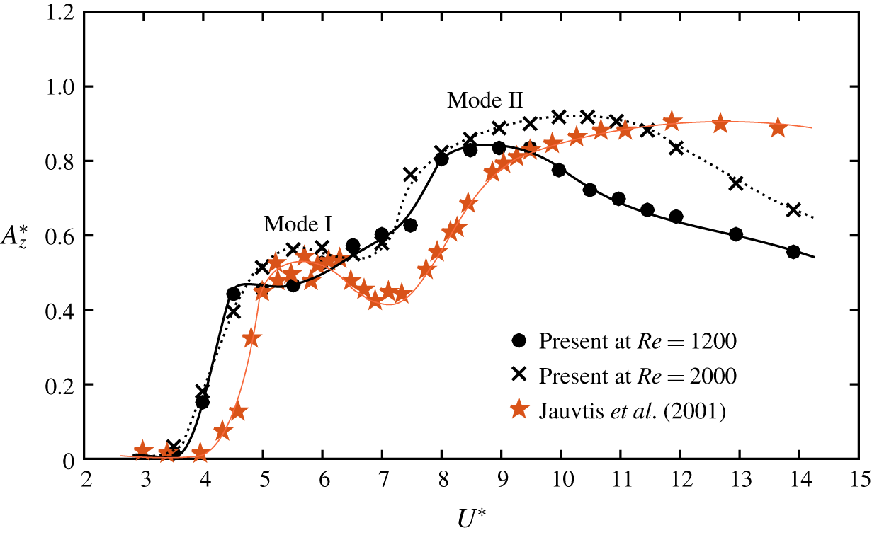
 $l^{\ast }=10$ was investigated by fixing the Reynolds number at a particular value. The sphere showed large-amplitude modes I and II vibration states at the larger Reynolds numbers investigated, similar to the observation of previous experimental studies. Figure 3 compares our results of the sphere vibration amplitude,
 $A_{z}^{\ast }=\sqrt{2}Z_{rms}/D$, at
 $Re=1200$ and
 $2000$ with the experimental results of Jauvtis et al. (Reference Jauvtis, Govardhan and Williamson2001) conducted with a sphere of the same mass ratio, where
 $Z$ is the sphere displacement in the
 $z$ direction. As can be seen, the present results match reasonably well with those of Jauvtis et al. Recall that, in the experiments, the Reynolds number was not fixed and varied approximately between
 $2000$ and
 $14\,000$. Consistent with their observations, the sphere response amplitudes at modes I and II were approximately
 $0.5D$ and
 $0.85D$, respectively.
Comparison of the sphere response amplitude,  $A_{z}^{\ast }$, at
 $Re=1200$ and
 $2000$ with the experimental results of Jauvtis et al. (Reference Jauvtis, Govardhan and Williamson2001) at higher and varying Reynolds numbers with a sphere of mass ratio
 $m^{\ast }=0.8$ over the reduced velocity range
 $U^{\ast }=[3,14]$. Consistent with their observations, the first two modes of sphere vibration states were observed.

In particular, at this mass ratio, Jauvtis et al. (Reference Jauvtis, Govardhan and Williamson2001) observed two peaks in the amplitude response curve, corresponding to modes I and II. In contrast, at  $Re=1200$, the sphere response amplitude varied smoothly from mode I to mode II without a dip as seen in most of the amplitude response curves of tethered spheres (Jauvtis et al. Reference Jauvtis, Govardhan and Williamson2001; Govardhan & Williamson Reference Govardhan and Williamson2005). However, once the Reynolds number is increased to
 $2000$, the response curve formed a small peak for mode I as observed by Jauvtis et al. Therefore, if the Reynolds number is further increased, this local peak at mode I is expected to become more prominent. At
 $Re=1200$, the highest vibration amplitude occurred around
 $U^{\ast }=8.5$, and the vibration amplitude decreased beyond this point, in contrast to the observation of Jauvtis et al. (Reference Jauvtis, Govardhan and Williamson2001) of almost constant amplitude at larger
 $U^{\ast }$ values. However, as the Reynolds number is increased to
 $2000$, the response amplitudes were higher than at
 $Re=1200$. Moreover, the response curve was closer to their response curve. Again, if the Reynolds number is further increased, the response curve at mode II is also anticipated to become more similar to the response curve of Jauvtis et al. observed at higher and varying Reynolds numbers. These observations show that there is a considerable effect of Reynolds number on the sphere response in this Reynolds-number range. Rajamuni et al. (Reference Rajamuni, Thompson and Hourigan2018a) also showed that there is a substantial effect of the Reynolds number on FIV of an elastically mounted sphere with one degree of freedom (DOF) in the laminar regime.
Compared to the observation of Jauvtis et al. (Reference Jauvtis, Govardhan and Williamson2001), the predicted response curves look slightly shifted to the left. However, the response that was predicted at  $U^{\ast }=4$ is not a periodic response as in mode I, albeit the shedding frequency is locked in to the oscillation frequency. Similar to the results of Jauvtis et al., we also expected mode I to occur around
 $U^{\ast }=5$ as the static vortex shedding frequency is
 $f_{vor}\approx 0.2$. Therefore, at
 $U^{\ast }=4$, the sphere may be in transition from no oscillation to VIV. Nonetheless, we observed mode I vibration at a slightly lower reduced velocity compared to that observed by Jauvtis et al. (Reference Jauvtis, Govardhan and Williamson2001). This difference may be due to the effect of Reynolds number. Note that, for the predictions, the Reynolds number was fixed, whereas it was allowed to vary with
 $U^{\ast }$ in the experiments.
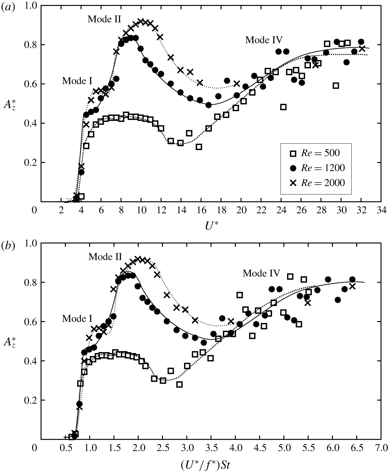
The sphere response curves at  $Re=500$ and
 $1200$ of a tethered sphere of
 $m^{\ast }=0.8$: the normalized amplitude,
 $A_{z}^{\ast }$, plotted against (a) the reduced velocity,
 $U^{\ast }$, and (b) the normalized velocity,
 $(U^{\ast }/f^{\ast })St$.

To explore the effect of Reynolds number in the laminar regime, another set of simulations was conducted at  $Re=500$ with the same mass ratio and tether length. Figure 4(a) shows a comparison of the sphere response amplitude of
 $Re=500$,
 $1200$ and
 $2000$ for the reduced velocity range
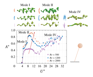
 $U^{\ast }=[3,32]$. As can be seen, the sphere response amplitude increased globally as the Reynolds number increased over
 $U^{\ast }\in [4.5,16]$. As discussed earlier, it showed periodic mode I and II vibrations over
 $U^{\ast }\approx [4.5,7]$ and
 $[8,16]$, respectively, at
 $Re=1200$ and
 $2000$. At
 $Re=500$, a periodic vibration response was found over
 $U^{\ast }=[4.5,12]$. The response curve took a bell shape with a maximum amplitude of
 ${\approx}0.45D$. At this Reynolds number, modes I and II were not able to be distinguished clearly from the amplitude response curve alone. Govardhan & Williamson (Reference Govardhan and Williamson2005) found that mode I occurred around
 $(U^{\ast }/f^{\ast })St=1$ while mode II occurred in the range of
 $(U^{\ast }/f^{\ast })St\approx [1.4,2]$. However, if the amplitude is plotted against
 $(U^{\ast }/f^{\ast })St$, both modes I and II responses became clear, even at
 $Re=500$, from the range of
 $(U^{\ast }/f^{\ast })St$ (see figure 4b).
Similar to the  $Re=500$ case, Rajamuni et al. (Reference Rajamuni, Thompson and Hourigan2018a) also observed bell-shaped response curves at
 $Re=300$ and
 $800$ with an elastically mounted sphere; these were named ‘branch A’. Moreover, the maximum amplitudes they observed at those Reynolds numbers were
 ${\approx}0.4D$ and
 $0.6D$, respectively. This observation leads to the conclusion that a sphere displays a trend of increasing amplitude globally over
 $U^{\ast }\approx [4,16]$, as the Reynolds number increased from
 $300$ to
 $2000$, regardless of whether it was an elastically mounted or a tethered sphere.
For  $U^{\ast }>16$, the sphere showed an aperiodic response for all three Reynolds numbers. Although the amplitudes were scattered, they showed initially an increasing trend and then levelling off around
 $0.8D$ as the reduced velocity increased to
 $34$. Rajamuni et al. (Reference Rajamuni, Thompson and Hourigan2018a) also reported a similar behaviour at
 $Re=800$ for
 $U^{\ast }>13$, but with a purely increasing trend up to
 $U^{\ast }=50$. As Rajamuni et al. claimed, this intermittent burst of vibration strongly resembles mode IV vibration discovered by Jauvtis et al. (Reference Jauvtis, Govardhan and Williamson2001) with a heavy sphere of
 $m^{\ast }=80$ for
 $U^{\ast }>100$. This begs the question: ‘Why is mode IV observed just after mode II without an intervening mode III?’ A discussion of this is given in § 4.3.
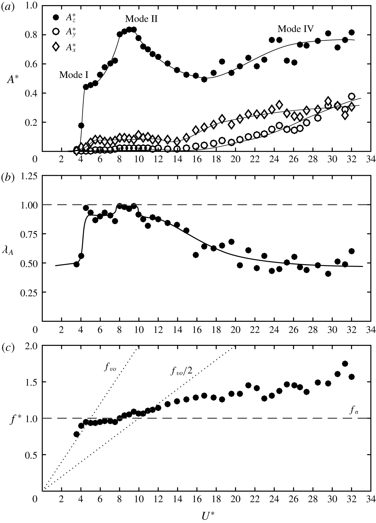
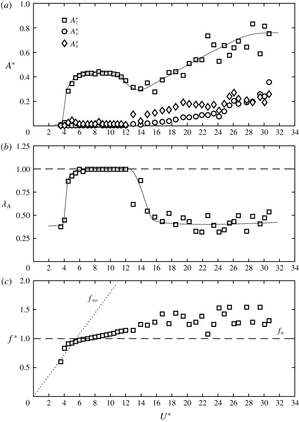
The FIV response of a tethered sphere at  $Re=1200$ over the reduced velocity range
 $U^{\ast }=[3,32]$: (a) sphere vibration amplitudes
 $A_{x}^{\ast }$,
 $A_{y}^{\ast }$ and
 $A_{z}^{\ast }$ in the streamwise, lateral and transverse directions, respectively; (b) the periodicity of the sphere vibration,
 $\unicode[STIX]{x1D706}_{A}=\sqrt{2}Z_{rms}/Z_{max}$; and (c) frequency ratio,
 $f^{\ast }=f/f_{n}$.

Williamson & Govardhan (Reference Williamson and Govardhan1997) and Govardhan & Williamson (Reference Govardhan and Williamson2005) identified that the motion of a tethered sphere is principally in the transverse direction. Consistently, we also observed large-amplitude vibrations in the transverse ( $z$) direction compared to the streamwise (
 $x$) and lateral (
 $y$) directions (see figures 5a and 6a). For mode I and II regimes, the sphere showed a negligible amplitude in the lateral direction while displaying a small amplitude of
 ${\approx}0.08D$ in the streamwise direction, as shown in figure 5(a) at
 $Re=1200$. This is consistent with the observation of Williamson & Govardhan (Reference Williamson and Govardhan1997) with a sphere of
 $m^{\ast }=0.73$ and tether length ratios
 $l^{\ast }=8.9$ and
 $3.8$.
The periodicity of the sphere vibration,  $\unicode[STIX]{x1D706}_{A}$, is defined as
 $\sqrt{2}Z_{rms}/Z_{max}$, where
 $Z_{max}$ is the maximum amplitude observed at each
 $U^{\ast }$. According to this definition,
 $\unicode[STIX]{x1D706}_{A}$ take values from
 $0$ to
 $1$, with
 $\unicode[STIX]{x1D706}_{A}=1$ representing the most periodic response. For both modes I and II, the sphere vibrations were highly periodic. However, the vibration was more periodic at the peak of mode II compared with the response at mode I (see figures 5b and 7a,c). For both modes I and II, the sphere vibrated in synchrony with the vortex shedding frequency,
 $f_{s}$, and was close to the system’s natural frequency, as expected (see figure 5c). Govardhan & Williamson (Reference Govardhan and Williamson1997, Reference Govardhan and Williamson2005) observed for light spheres (
 $m^{\ast }<1$) across the mode II regime and above that the dynamic vortex shedding frequency remained between the static body vortex shedding frequency,
 $f_{vor}$, and the natural frequency of the system.
The FIV response of a tethered sphere at  $Re=500$ over the reduced velocity range
 $U^{\ast }=[3,32]$: (a) sphere vibration amplitude,
 $A^{\ast }$; (b) the periodicity of the sphere vibration,
 $\unicode[STIX]{x1D706}_{A}=\sqrt{2}Z_{rms}/Z_{max}$; and (c) frequency ratio,
 $f^{\ast }=f/f_{n}$.

As the sphere response curve for  $Re=500$ deviated from the response curve observed at higher Reynolds numbers over the mode I and II regimes (
 $U^{\ast }=[4.5,12]$), a negligible amplitude was observed in both the streamwise (
 $x$) and lateral (
 $y$) directions (see figure 6a). Vibrations in the transverse (
 $z$) directions were highly periodic as in the peak of mode II (figure 6b). This is indeed a VIV response (
 $f=f_{s}=f_{n}$). From these observations, we can predict that the response of a tethered sphere collapses well with the response of an elastically mounted sphere of one DOF for low Reynolds numbers over the modes I and II regimes.
As the reduced velocity increased beyond  $U^{\ast }=12$ (beyond the mode II regime), the periodicity of the sphere response gradually decreased at
 $Re=1200$ and reached a value of
 ${\approx}0.5$ for the mode IV regime (see figure 5b). A similar behaviour was observed at
 $Re=500$ as well. However, as
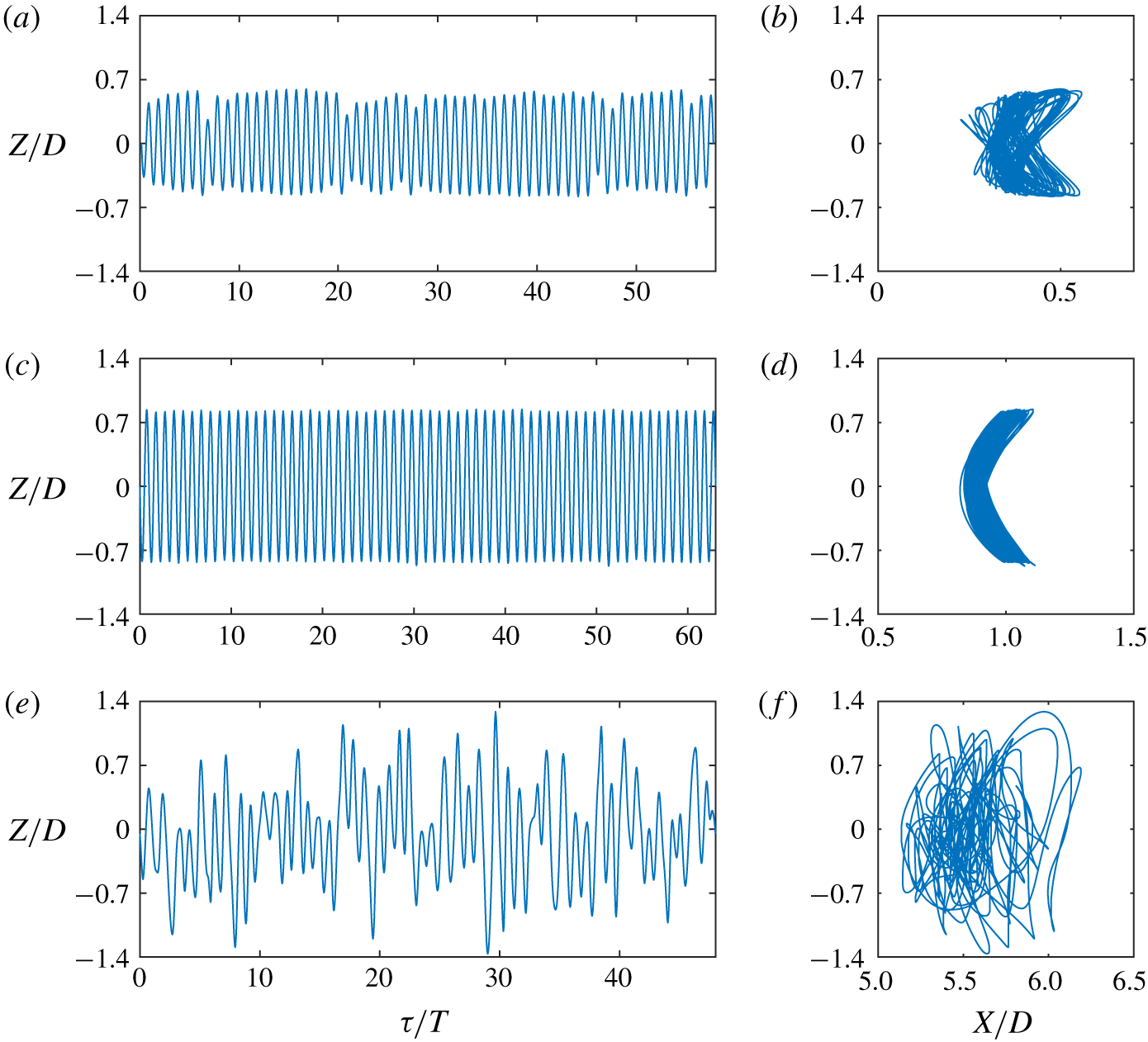
 $U^{\ast }$ was increased, mode IV appeared quickly after the periodic vibrations and the periodicity of the response was even lower. The sphere vibration was intermittent in mode IV, as shown in figure 7(e) at
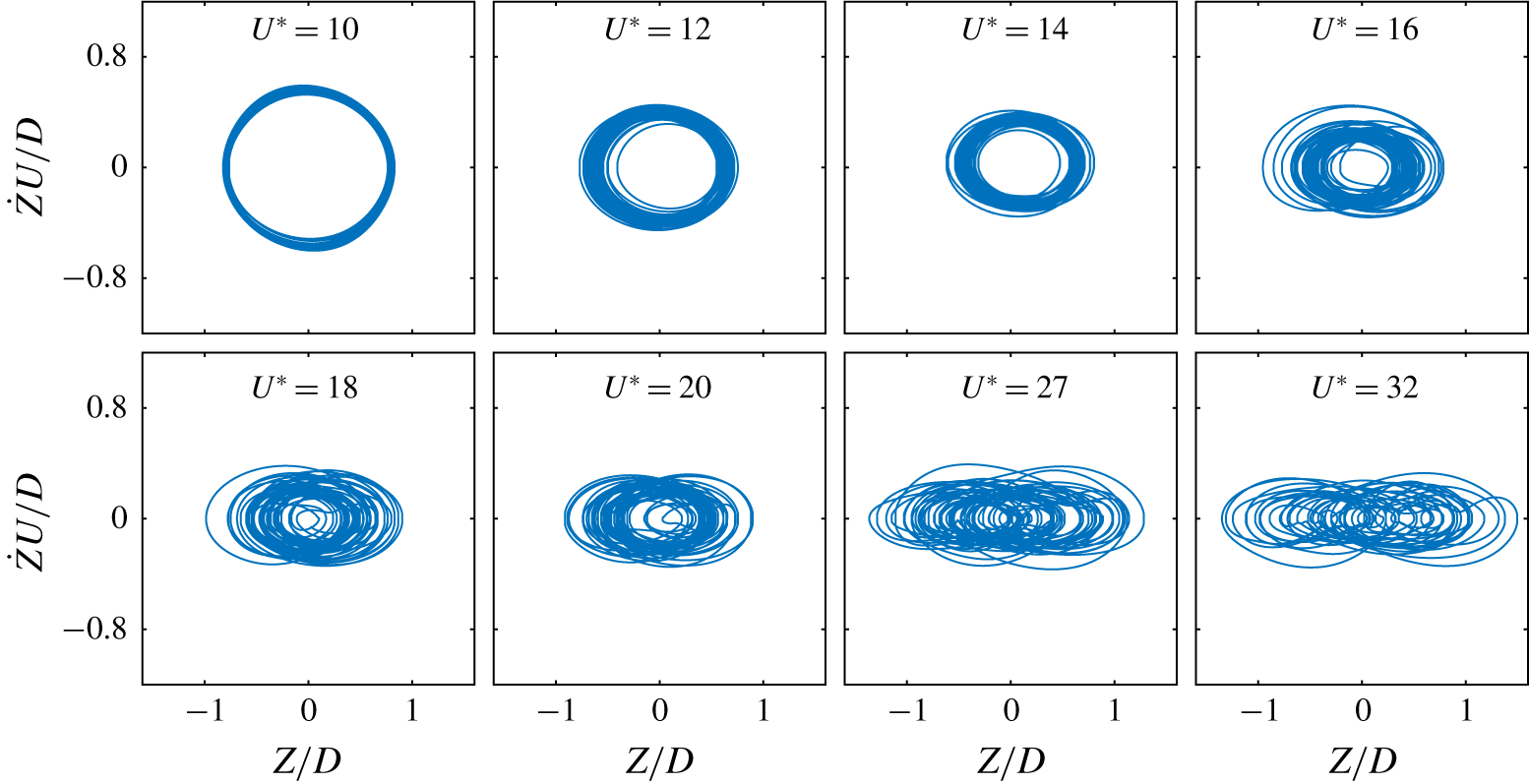
 $U^{\ast }=27.4$, and it followed an irregular trajectory without a clear pattern, as shown in figure 7(f). As
 $\unicode[STIX]{x1D706}_{A}$ decreased, the sphere displacement in the streamwise and lateral directions became slightly more significant. The streamwise amplitude was almost a constant value of
 ${\approx}0.3D$ at
 $Re=1200$ and
 ${\approx}0.2D$ at
 $Re=500$ over mode IV. The lateral amplitude showed a linearly increasing trend as the reduced velocity increased beyond
 $16$ and was almost half the transverse amplitude at the highest reduced velocity considered (
 $U^{\ast }=32$) at both Reynolds numbers. This shows that the randomness of the signal increases with reduced velocity.
(a,c,e) Time histories and (b,d,f) sphere trajectories in the  $x$–
 $z$ plane at
 $Re=1200$, where
 $\unicode[STIX]{x1D70F}=tU/D$ is the non-dimensional time and
 $T$ is the period: (a,b) at
 $U^{\ast }=6$ (mode I), (c,d) at
 $U^{\ast }=9$ (mode II), and (e,f) at
 $U^{\ast }=27.4$ (mode IV).

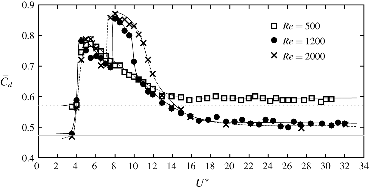
Figure 8 displays the time-averaged drag coefficient,  $\overline{C}_{d}$, as a function of the reduced velocity for all three Reynolds numbers considered. An increment in
 $\overline{C}_{d}$ is observed when it vibrated periodically, as found in previous experimental and numerical studies (Gottlieb Reference Gottlieb1997; Williamson & Govardhan Reference Williamson and Govardhan1997; Behara et al. Reference Behara, Borazjani and Sotiropoulos2011). At
 $Re=500$, as the sphere began to vibrate at
 $U^{\ast }=4.5$, an
 ${\sim}33\,\%$ increment of
 $\overline{C}_{d}$ was observed from the value for a stationary sphere. Similar to the observation of Rajamuni et al. (Reference Rajamuni, Thompson and Hourigan2018a) for their branch A, this increment then decreased over the synchronization regime. However, they observed a sharp turn at the beginning of the range, while we observed a smooth turn. At both
 $Re=1200$ and
 $2000$,
 $\overline{C}_{d}$ showed another jump at the beginning of mode II, as Govardhan & Williamson (Reference Govardhan and Williamson1997) observed. The increments of
 $\overline{C}_{d}$ were
 ${\sim}60\,\%$ and
 ${\sim}100\,\%$ at modes I and II, respectively. In the mode IV regime, even larger-amplitude vibrations are observed, whereas the drag coefficient hardly changed at all. This is because mode IV is not a VIV response, as discussed in § 4.4.
Variation of the time-averaged drag coefficient,  $\overline{C}_{d}$, with the reduced velocity at
 $Re=500$,
 $1200$ and
 $2000$. The horizontal grey lines show
 $\overline{C}_{d}$ calculated with a stationary sphere at
 $Re=500$ (dotted line) and
 $Re=1200$ (solid line).

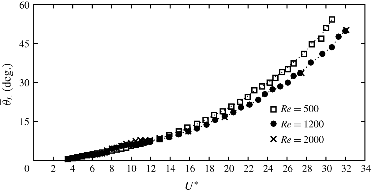
The time-mean layover angle,  $\bar{\unicode[STIX]{x1D703}}_{L}$ (angle of tether from the
 $y$ direction), as a function of reduced velocity. The dotted lines represent the estimated
 $\bar{\unicode[STIX]{x1D703}}_{L}$ from the drag coefficient at each Reynolds number.

The time-mean layover angle,  $\overline{\unicode[STIX]{x1D703}}_{L}$, is defined as the angle of the tether to the lateral direction (vertical). An exponentially increasing trend of
 $\overline{\unicode[STIX]{x1D703}}_{L}$ with a slight variation in mode II was observed for all of the Reynolds numbers considered (see figure 9). Since the lift force is comparatively small, the layover angle can be estimated from the non-dimensional drag and buoyancy forces as
 $$\begin{eqnarray}\displaystyle \tan (\bar{\unicode[STIX]{x1D703}}_{L})=\frac{C_{d}}{(1-m^{\ast })\unicode[STIX]{x1D6FC}}. & & \displaystyle\end{eqnarray}$$
As can be seen in figure 9, the calculated  $\overline{\unicode[STIX]{x1D703}}_{L}$ is coincident with the estimated values. Note that, even though
 $\overline{C}_{d}$ is constant over the mode IV regime,
 $\tan (\unicode[STIX]{x1D703}_{L})$ increases; this is because
 $\unicode[STIX]{x1D6FC}=4/(3Fr^{2})$ is not constant in this numerical study.
In this study, the tether was assumed rigid and the torsion of the sphere was neglected. However, it is worth exploring the nature of the sphere response when the sphere is allowed to rotate through the axis of the tether, according to the moment acting on it. Nevertheless, the moments acting on the sphere were found to be negligible compared to the forces acting on it (moments  ${<}1\,\%$ forces). Thus, it can be assumed that the sphere undergoes a very small amount of rotation when it is also subjected to torsion. Our previous study (Rajamuni et al. Reference Rajamuni, Thompson and Hourigan2018b) and the study of Sareen et al. (Reference Sareen, Zhao, Lo Jacono, Sheridan, Hourigan and Thompson2018a) investigated the VIV response of an elastically mounted sphere under a forced rotation. Both of these studies found that the effect of rotation is negligible on the VIV response of the sphere, for small rotation rates. The investigation of Sareen et al. (Reference Sareen, Zhao, Sheridan, Hourigan and Thompson2018c) also found that the rotary motion of the sphere has a negligible effect on the VIV response of a sphere, for small velocity ratios. This combined evidence indicates that the VIV response of a tethered sphere is highly unlikely to be altered by the sphere torsion.
From the findings of this study and previous experimental and numerical studies, a brief discussion of the different modes of sphere vibrations is provided in the following three subsections.
4.2 Modes I and II
Modes I and II are the only VIV responses observed for a sphere out of the four vibration modes found. Mode I response is due to a natural resonance, where the vibration of the sphere is excited when the natural frequency of the system,  $f_{n}$, is close to the stationary-body (non-VIV) vortex shedding frequency. For example, at
 $Re=1200$, the vortex shedding frequency of a stationary sphere,
 $f_{vor}$, is approximately
 $0.2$, which means that the natural oscillation frequency and the stationary-body vortex shedding frequency coincide at
 $U^{\ast }=5$. As a result of this, mode I was observed close to
 $U^{\ast }=5$ (see figure 5a).
In almost all of the VIV studies, the sphere showed large-amplitude periodic vibrations even after the resonance range, and this is known as the mode II vibration state. As the sphere is allowed to translate freely, a reduction is observed in the vortex shedding frequency from the value for a static sphere. In this manner, the dynamic shedding frequency deviated from the static shedding frequency and synchronized with the natural frequency (see figures 5c and 6c). As a result, the sphere showed large-amplitude vibration (mode II) after the resonance state.
The mode II response was observed beyond the mode I regime as the reduced velocity was increased. The sphere response amplitude varied smoothly as the vibration state transitioned from mode I to mode II, in contrast to the distinct branches observed in the amplitude response curve of an elastically mounted cylinder (one DOF). The sphere response curve showed a small local peak in mode I for light tethered spheres ( $m^{\ast }<1$); for example, the observations of Williamson & Govardhan (Reference Williamson and Govardhan1997) at
 $m^{\ast }=0.729$ with both
 $l^{\ast }=3.83$ and
 $8.93$ and at
 $m^{\ast }=0.082$ with
 $l^{\ast }=9.28$, those of Govardhan & Williamson (Reference Govardhan and Williamson1997) at
 $m^{\ast }=0.26$, and those of Jauvtis et al. (Reference Jauvtis, Govardhan and Williamson2001) at
 $m^{\ast }=0.8$, can be mentioned. However, the local peak in mode I is obscured for heavy spheres (
 $m^{\ast }>1$), especially for elastically mounted spheres, as discussed by Govardhan & Williamson (Reference Govardhan and Williamson2005). The range of
 $U^{\ast }$ values varies for different modes; mode I is observed for a very short range (within
 ${\sim}(1{-}2)U^{\ast }$) compared with mode II. This is expected, as mode I is the result of resonance.
The difference between modes I and II was studied by Govardhan & Williamson (Reference Govardhan and Williamson2005) by analysing the phase between sphere oscillation and the fluid forces acting on the sphere. Lighthill (Reference Lighthill1986) showed that the total fluid force,  $F_{t}$, can conveniently be split into two components, a ‘potential force’ component (
 $F_{p}$) related to the potential added mass and a ‘vortex force’ component (
 $F_{v}$) related to the dynamic vorticity. For a cylinder, Govardhan & Williamson (Reference Govardhan and Williamson2000) found a shift in the total phase,
 $\unicode[STIX]{x1D719}_{t}$ (the phase between the sphere displacement and the total force), or the vortex phase,
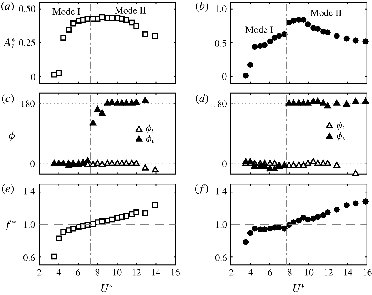
 $\unicode[STIX]{x1D719}_{v}$ (the phase between the sphere displacement and the vortex force), as the vibration state transitions from one branch to another. Analogously, Govardhan & Williamson (Reference Govardhan and Williamson2005) observed a shift in the vortex phase, while the total phase remains almost constant, as the sphere transitions from mode I to mode II. In a similar fashion, we found that the vortex phase shifted from
 $0^{\circ }$ to
 $180^{\circ }$ as the vibration state transitioned from mode I to mode II, while the total phase remained at
 ${\approx}0^{\circ }$, as shown in figure 10(c,d) for
 $Re=500$ and
 $1200$, respectively.
For an elastically mounted cylinder, Govardhan & Williamson (Reference Govardhan and Williamson2000) argued that a sudden shift in total or vortex phase can be expected as the body oscillation frequency passes the natural frequency of the system (or the frequency ratio crosses the  $f^{\ast }=1$ line). Consistent with this argument, we observed that the shift in
 $\unicode[STIX]{x1D719}_{v}$ occurs as the frequency ratio crosses the
 $f^{\ast }=1$ line (see figure 10e,f). In addition to this, Govardhan & Williamson discussed that, for a purely sinusoidal response with zero damping ratio, the total or vortex force can only be either phase-aligned or be
 $180^{\circ }$ out of phase with the body vibration. That discussion related to an elastically mounted cylinder. The motion of a tethered sphere has no damping effect (see equation (2.21)). Therefore, if the sphere response is periodic, we can predict that
 $\unicode[STIX]{x1D719}_{t}$ and
 $\unicode[STIX]{x1D719}_{v}$ can be either
 $0^{\circ }$ or
 $180^{\circ }$ in a similar way. Consistently, we observed that
 $\unicode[STIX]{x1D719}_{t}$ and
 $\unicode[STIX]{x1D719}_{v}$ were mostly either
 $0^{\circ }$ or
 $180^{\circ }$.
Variation of (a,b) sphere response amplitude, and (c,d) the total phase,  $\unicode[STIX]{x1D719}_{t}$, and vortex phase,
 $\unicode[STIX]{x1D719}_{v}$, over modes I and II regimes. (e,f) The frequency ratio crosses the
 $f^{\ast }=1$ line as the vortex phase shifts from
 $0^{\circ }$ to
 $180^{\circ }$. Column (a,c,e) for
 $Re=500$ and (b,d,f) for
 $Re=1200$.

The response amplitude of mode II was found to be higher than the amplitude of mode I (for some cases, approximately twice the amplitude of mode I) by experimental studies at higher Reynolds numbers. We also observed a similar behaviour at  $Re=1200$ and
 $2000$. However, for
 $Re<1000$, the amplitude of mode II was observed to be similar to that of mode I (present study at
 $Re=500$ and Rajamuni et al. (Reference Rajamuni, Thompson and Hourigan2018a) at
 $Re=300$ and
 $800$). Therefore, the effect of Reynolds number on the amplitude of mode II is not negligible in the laminar regime.
4.2.1 Effect of Reynolds number
Govardhan & Williamson (Reference Govardhan and Williamson2005) showed that the effect of Reynolds number is negligible for the VIV of a sphere over a range of  $Re\in [2000,12\,000]$ with the help of the Griffin plot and the tether length ratio. However, the effect of Reynolds number is significant over
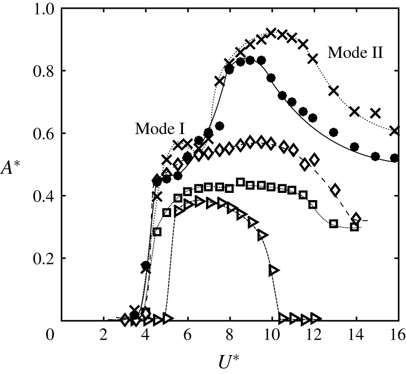
 $Re\in [300,2000]$. Figure 11 plots the sphere predicted responses together with the results of Rajamuni et al. (Reference Rajamuni, Thompson and Hourigan2018a) with elastically mounted spheres at five different Reynolds numbers over modes I and II regimes. As can be seen, the response amplitude increases globally with the Reynolds number. This effect is more significant over the mode II regime than the mode I regime. In addition, the mode II regime widened as the Reynolds number increased in this range. Mode II appears to be more sensitive to the Reynolds number.
The amplitude response curves at different Reynolds numbers at the modes I and II regimes: ▹, at  $Re=300$ of Rajamuni et al. (Reference Rajamuni, Thompson and Hourigan2018a) with an elastically mounted sphere of
 $m^{\ast }=2.865$; ▫, at
 $Re=500$; ♢, at
 $Re=800$ of Rajamuni et al. (Reference Rajamuni, Thompson and Hourigan2018a) with an elastically mounted sphere of
 $m^{\ast }=2.865$; ●, at
 $Re=1200$; and
 $\boldsymbol{\times }$ at
 $Re=2000$.

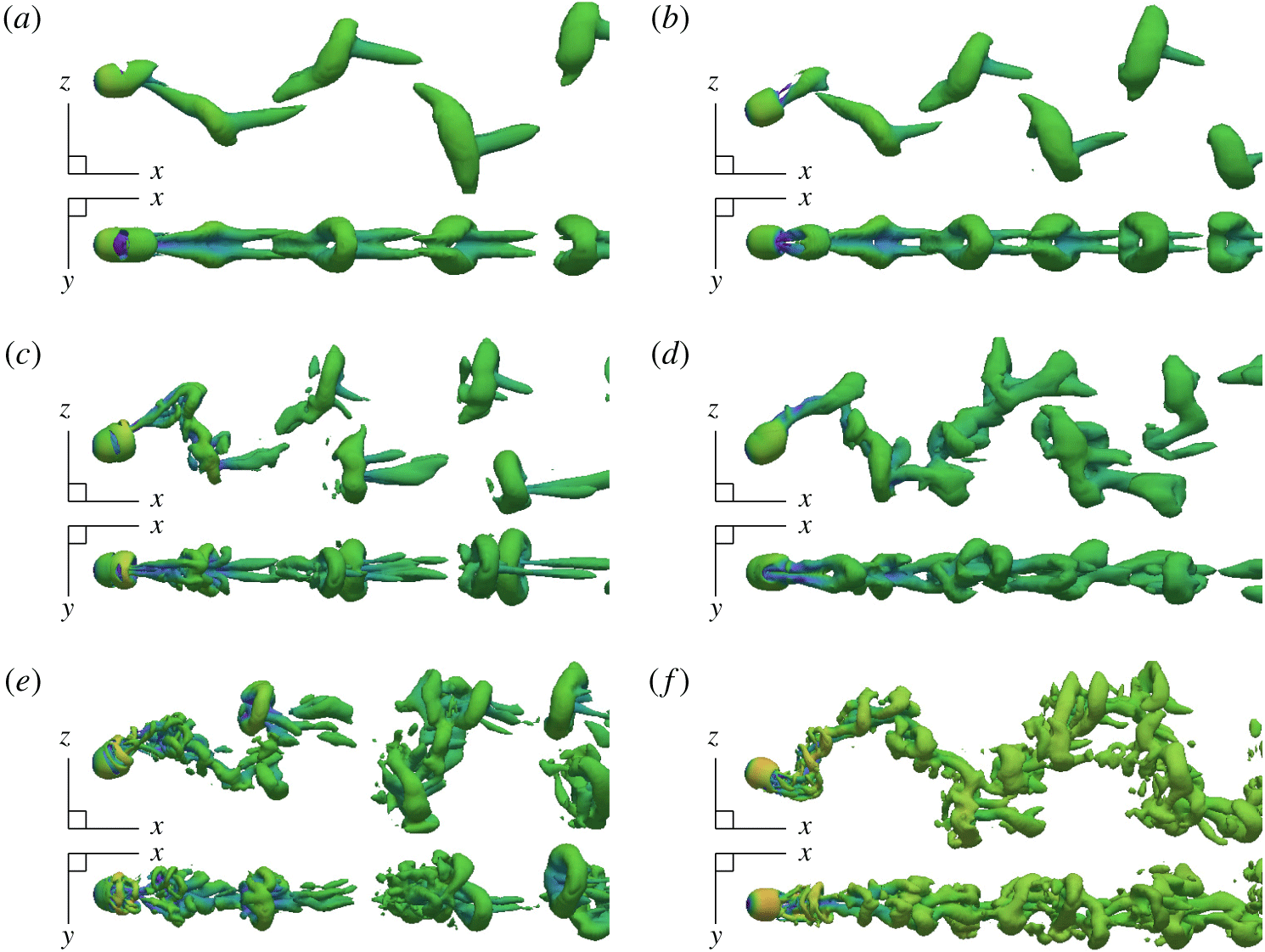
Wake structures in modes I and II at  $Re=500$,
 $1200$ and
 $2000$ visualized with isosurface of
 $Q$ at
 $0.01$. Flow from left to right.

Results of DMD analysis of the 2-D velocity field over  $10$ oscillation cycles of mode I at
 $Re=500$: (a) plot of eigenvalues of the companion matrix; (b) frequency spectrum; (c–f) dynamic modes KM (visualized by vorticity field) corresponding to frequencies
 $f_{0}$,
 $f_{1}$,
 $2f_{1}$ and
 $3f_{1}$, respectively; (g) actual vorticity field; (h–j) reconstructions of the vorticity field using all the KMs, only the dominant KM (
 $f_{0}+f_{1}$), and the dominant KM and its higher-order harmonics (
 $f_{0}+f_{1}+2f_{1}+3f_{1}+4f_{1}+5f_{1}+6f_{1}$), respectively.

4.2.2 Effect of mass ratio
Govardhan & Williamson (Reference Govardhan and Williamson2005) studied the effect of mass ratio on the sphere response and found that the response amplitude increased and the synchronization regime widened as the mass ratio decreased over the range  $m^{\ast }\in [2.8,198.4]$. For light spheres (
 $m^{\ast }<1$), once the sphere reached its maximum amplitude (in mode II) by diverging from the usual decreasing trend, a levelling-off trend was observed in experiments. For example, see Williamson & Govardhan (Reference Williamson and Govardhan1997) at
 $m^{\ast }=0.729$, Govardhan & Williamson (Reference Govardhan and Williamson2005) at
 $m^{\ast }=0.45$ and Jauvtis et al. (Reference Jauvtis, Govardhan and Williamson2001) at
 $m^{\ast }=0.8$. However, in this numerical study, we observed a decreasing trend of amplitude after the maximum amplitude at
 $m^{\ast }=0.8$. This difference from the experiments is most probably due to the effect of Reynolds number. We showed that the effect of Reynolds number is higher in the mode II regime. Therefore, if
 $Re$ was increased further, there is an expectation that there will be a levelling-off trend towards the end of mode II. In addition, for light spheres and mode II, the shedding frequency was slightly higher than the natural frequency of the system.
4.2.3 Wake structure
The vortical structures of the wake were visualized with an isosurface of the  $Q$-criterion (the second invariant of the velocity tensor) introduced by Hunt, Wray & Moin (Reference Hunt, Wray and Moin1988). The wake structures observed in modes I and II regimes are shown in figure 12 and in supplementary movies (available online at https://doi.org/10.1017/jfm.2019.928). As can be seen, at
 $Re=500$, two trails of hairpin vortices form the wake in both modes I and II regimes. These wake structures strongly resemble the wakes observed by Govardhan & Williamson (Reference Govardhan and Williamson2005) for modes I and II, and by Rajamuni et al. (Reference Rajamuni, Thompson and Hourigan2018a) for their branch A. Two hairpin loops were shed per sphere oscillation cycle and these loops were disconnected and two-sided. Furthermore, each vortex loop was accompanied by a tail. These hairpin loops were symmetric through the
 $x$–
 $z$ plane as expected. Govardhan & Williamson (Reference Govardhan and Williamson2005) explained that the two streamwise vortex loops associated with the orientation of the hairpin loops create a lift force similar to the vertical lift force associated with aircraft trailing ‘tip vortices’. As the hairpin loops are two-sided, the lift force is periodic and hence the sphere is excited to vibrate.
As the Reynolds number is increased, small-scale structures begin to appear in the wake. In mode I, the underlying wake structure was only slightly modified, continuing to show two strong hairpin loops per oscillation cycle, along with smaller-scale structures. However, in mode II, the wake was modified further. Multiple loops were observed per oscillation cycle in the higher-Reynolds-number cases. Moreover, those loops were mostly connected with each other.
4.2.4 Dynamic mode decomposition
For further examination of the wake, and to identify the dominant wake modes, DMD was performed. The nature of the wake of mode I ( $U^{\ast }=5.5$) was studied at
 $Re=500$ using the two-dimensional (2-D) velocity field (on the
 $x$–
 $z$ plane) over 10 oscillation cycles with 23 snapshots per cycle. As figure 13(a) shows, the plot of eigenvalues of the companion matrix lies in a unit circle, indicating a periodic wake. Moreover, the frequency,
 $f_{1}$, of the dynamic mode with the highest magnitude was identical to the oscillation frequency of the sphere, as expected. The sphere oscillation was not purely sinusoidal in this case; therefore, the frequency spectrum contained other frequencies besides the dominant frequency and its higher-order harmonics (see figure 13b). The vorticity field was used to visualize the Koopman modes (KMs), and to compare the reconstruction using these modes with the actual field (see figure 13c–j). The reconstruction with all modes, shown in figure 13(h), is identical to the actual field shown in figure 13(g), providing some validation to the analysis. The dominant KM has captured the main features of the field (see figure 13i). Moreover, when its higher-order harmonics are also used, it looks much closer to the actual field – compare figure 13(j) and (g).
The DMD analysis of the 2-D velocity field of mode II ( $U^{\ast }=9$) at
 $Re=1200$ over
 $24$ oscillation cycles with
 $48$ snapshots per cycle was performed, and results are presented in figure 14. The plot of eigenvalues of the companion matrix provides evidence of a highly periodic wake. The sphere oscillation is purely sinusoidal in mode II. Inferred from this, the frequency spectrum in mode II for
 $Re=500$ (not shown) contained only the dominant frequency and its higher-order harmonics. However, as
 $Re$ was increased to
 $1200$, the frequency spectrum was dense with other frequencies, showing the effect of Reynolds number (see figure 14b). Nevertheless, the underlying streamwise vortex structure observed for the dominant KM (see figure 14e) was synchronized with the sphere oscillation, so the sphere showed large-amplitude mode II vibrations. This was also clearly visible from the isosurfaces of
 $Q$ when 3-D velocity fields were used for the analysis, as shown in figure 15 for both modes I and II.
Results of DMD analysis of the 2-D velocity field over  $24$ oscillation cycles of mode II at
 $Re=1200$: (a) plot of eigenvalues of the companion matrix; (b) frequency spectrum; (c) actual vorticity field; (d–f) reconstructions of the vorticity field using all the KMs, only the dominant KM (
 $f_{0}+f_{1}$), and the dominant KM and its higher-order harmonics (
 $f_{0}+f_{1}+2f_{1}+3f_{1}+4f_{1}$), respectively.

Isosurfaces of the wake at modes I and II reconstructed from all of the KMs (a,b) and with only the dominant KM (c,d). The dominant KM has captured the main feature of the flow.

4.2.5 Robustness of modes I and II
Earlier, we showed that mode II is quite sensitive to the Reynolds number for  $Re\in [300,2000]$. In addition, mode II also appears sensitive to disturbances and other factors. For example, the experimental study of Sareen et al. (Reference Sareen, Zhao, Lo Jacono, Sheridan, Hourigan and Thompson2018a) and the computational study of Rajamuni et al. (Reference Rajamuni, Thompson and Hourigan2018b) found that the mode II response weakens if even weak rotation (in the transverse direction) is imposed on the sphere. In particular, they observed a considerable reduction in the maximum oscillation amplitude and a narrowing of the synchronization regime. Furthermore, Sareen et al. (Reference Sareen, Zhao, Lo Jacono, Sheridan, Hourigan and Thompson2018b) identified that the proximity of the sphere to the free surface greatly influences mode II. From these observations, we can conclude that mode I is more robust than mode II. Perhaps this is unsurprising, as mode I is the primary resonant response.
4.3 Mode III
After the mode II regime, Jauvtis et al. (Reference Jauvtis, Govardhan and Williamson2001) discovered another periodic vibration state, namely mode III. It was an unexpected finding that was first observed with a sphere of  $m^{\ast }=28$ with water channel experiments. To study this mode further, they performed a set of wind tunnel experiments with a tethered sphere of
 $m^{\ast }=80$ for a wide range of
 $U^{\ast }$. Mode III was found to occur after a desynchronization regime for a broad range of
 $U^{\ast }$ from
 $20$ to
 $40$. They repeated this set of experiments with a larger tunnel to check whether it was an experimental artifact. Mode III was evident even with the larger tunnel. In addition to that, it was observed with a sphere of
 $m^{\ast }=940$. The sphere response was remarkably periodic and the vibration amplitudes were almost the same as for mode II. Not only tethered spheres, but also elastically mounted spheres, showed mode III vibrations, but without a desynchronization regime; for example, this was found by Govardhan & Williamson (Reference Govardhan and Williamson2005) with
 $m^{\ast }=53.7$ and Sareen et al. (Reference Sareen, Zhao, Lo Jacono, Sheridan, Hourigan and Thompson2018a) with
 $m^{\ast }=14.2$.
As a consequence of the high mass ratio in previous experiments, the oscillation frequency of mode III was identical to the system’s natural frequency. Nevertheless, it was difficult to explain the existence of mode III, since the principal vortex shedding frequency is 3–8 times higher than the oscillation frequency. Govardhan & Williamson (Reference Govardhan and Williamson2005) observed multiple small-scale structures in the wake of mode III. There was no clear association between vortex shedding and full or half wavelength of the sphere vibration.
Mode III is not possible to explain with the classic lock-in theories and such a vibration state does not exist for the case of cylinder free vibration. Govardhan & Williamson (Reference Govardhan and Williamson2005) argued that the flow must create a forcing on the body at this low frequency, sufficient to deliver a net energy transfer to the body motion. They measured the streamwise vorticity using DPIV and found a two-sided chain of trailing vortex pairs that is locked in with the sphere frequency. With this observation, they claimed that there is a net positive energy transfer in the vibration over a cycle, enabling the highly periodic mode III. A tethered or an elastically mounted sphere is intrinsically unstable. Govardhan & Williamson (Reference Govardhan and Williamson2005) argued that, if the sphere is perturbed in the transverse direction, it can generate a self-sustaining vortex force to enhance the body vibration, to possibly a large amplitude. In the mode III regime, the sphere is highly likely to be perturbed, as its wake is naturally responsive to low-frequency disturbances (Brücker Reference Brücker2001). Hence, Govardhan & Williamson (Reference Govardhan and Williamson2005) concluded that mode III is an example of ‘movement-induced vibration’, categorized by Naudascher & Rockwell (Reference Naudascher and Rockwell2012).
Compared to the first two vibration modes, mode III has been little examined; only a couple of studies have reported it, and its nature is not well understood yet. Therefore, further investigation is presented here. We attempt to enhance the understanding of mode III, through some previous experimental observations together with selected simulations.
We observed that the mode III state appears only with heavy spheres. In particular, Jauvtis et al. (Reference Jauvtis, Govardhan and Williamson2001) found mode III for spheres of  $m^{\ast }=28$,
 $80$ and
 $940$, while Govardhan & Williamson (Reference Govardhan and Williamson2005) observed it for spheres of
 $m^{\ast }=11.7$,
 $31.1$,
 $53.7$ and
 $75$, and Sareen et al. (Reference Sareen, Zhao, Lo Jacono, Sheridan, Hourigan and Thompson2018a) for a sphere of
 $m^{\ast }=14.2$. From this, we can hypothesize that mode III arises only for high-inertia systems (heavy spheres). We intended to check this hypothesis with a sphere of higher mass ratio. Unfortunately, simulations are very costly for higher-mass-ratio cases, since it takes a very long time to reach the steady state. Therefore, only a couple of runs were feasible.
At  $m^{\ast }=0.8$ and
 $Re=1200$, intermittent mode IV vibrations were observed for
 $U^{\ast }\in [16,32]$ just after mode II, without a trace of mode III. To study the possibility of mode III being excited, we performed a simulation with a sphere of
 $m^{\ast }=80$ at
 $U^{\ast }=30$ and
 $Re=1200$. This
 $U^{\ast }$ was chosen since mode III emerged predominantly for the reduced velocity range
 $U^{\ast }\in [20,40]$ in earlier experimental studies. Figure 16(a) shows the time history of the sphere displacement in this case. As can be seen, the sphere vibration has become fairly periodic from intermittent vibration as the mass ratio increased to
 $80$. The sphere response amplitude converged to a value of
 ${\approx}0.5D$ after a long transient period. The sphere vibration is highly periodic. Moreover, its frequency coincides with the system’s natural frequency, as expected at this high mass ratio. However, neither the total nor vortex forces were periodic, and those forces were small in magnitude with a high frequency (see figure 16b). As seen in previous experimental studies, the vortex shedding frequency was higher than the sphere frequency; for this case, it was approximately six times higher. Thus, this is essentially a mode III response. Figure 17 shows the wake structure observed. Figure 16(c,d) shows the sphere trajectory in
 $y$–
 $z$ and
 $x$–
 $z$ planes. Its displacement in the streamwise (
 $x$) and lateral (
 $y$) directions were negligible compared to the displacement in the transverse (
 $z$) direction. However, the streamwise frequency is the same as the transverse frequency, in contrast to modes I and II, for which the streamwise frequency is double the transverse frequency. Therefore, the sphere trajectory in mode III deviated from the figure ‘8’ shape to a figure ‘0’ shape. This indicates that mode III is essentially not an extension of mode II, but a completely different vibration state.
The sphere response at  $m^{\ast }=80$,
 $U^{\ast }=30$ and
 $Re=1200$: (a) time history; (b) sphere displacement together with total and vortex force coefficients,
 $C_{t}$ and
 $C_{v}$, respectively; and (c,d) trajectory of the sphere in
 $y$–
 $z$ and
 $x$–
 $z$ planes, respectively, at the steady state.

Wake observed in mode III ( $Re=1200$,
 $m^{\ast }=80$,
 $l^{\ast }=10$ and
 $U^{\ast }=30$) visualized with isosurface of
 $Q=0.001$. Flow from left to right.

The DMD analysis of mode III ( $Re=1200$,
 $m^{\ast }=80$) for
 $10$ oscillation cycles with
 $48$ snapshots per cycle: (a) plot of eigenvalues of the companion matrix; (b) frequency spectrum; and (c,d) isosurfaces of
 $Q$ using all KMs and only the dominant KM conjugate pair, respectively.

4.3.1 Dynamic mode decomposition
The wake of mode III was investigated with DMD using the velocity field over  $10$ sphere oscillation cycles, with
 $48$ snapshots per cycles. As figure 18(a) shows, eigenvalues of the companion matrix lie mainly on the unit circle, indicating a strong periodicity of the wake. Additionally, the dominant frequency of the wake, identified from the frequency spectrum shown in figure 18(b),
 $f_{1}=0.0335$, is identical to the sphere oscillation frequency. The frequency spectrum was dense with several frequencies, showing the effect of Reynolds number. Even though a number of small loops were shed per oscillation cycle, the wake displays a long-wavelength structure in the downstream direction corresponding to the sphere oscillation. Figure 18(c,d) shows the isosurfaces of
 $Q$ of the reconstructed field with all of the KMs and only the dominant KM pair, respectively. The reconstruction with only the dominant KM pair consists of long vortical structures, similar to the observation of Govardhan & Williamson (Reference Govardhan and Williamson2005). These long structures were also visible in the 2-D vorticity field (not shown).
4.3.2 The sphere response beyond the mode III regime
To compare with the results of Jauvtis et al. (Reference Jauvtis, Govardhan and Williamson2001) at higher  $U^{\ast }$ values, two more simulations were performed at
 $U^{\ast }=70$ and
 $150$. After mode III, they have observed a desynchronization regime for the
 $U^{\ast }$ range of
 ${\approx}[40,100]$ and then mode IV vibration for
 $U^{\ast }>100$ with a sphere of
 $m^{\ast }=80$. Consistent with their results, we observed a small-scale vibration at
 $U^{\ast }=70$ and mode IV at
 $U^{\ast }=150$ (see figure 19). As the mass ratio increased from
 $0.8$ to
 $80$, mode III vibration was predicted before mode IV and the ranges of these modes match well with the experimental result of Jauvtis et al. (Reference Jauvtis, Govardhan and Williamson2001). From these observations it is evident that mode III is essentially a movement-induced vibration, as Govardhan & Williamson (Reference Govardhan and Williamson2005) explained.
4.3.3 Effect of the mass ratio
The sphere response at  $m^{\ast }=80$ and
 $Re=1200$. (a) Comparison of the response amplitudes for
 $m^{\ast }=80$ calculated for
 $U^{\ast }=30$,
 $70$ and
 $150$ denoted by
 $\odot$ with the amplitude of
 $m^{\ast }=0.8$ denoted by ●. The dotted line shows the expected response amplitude curve for
 $m^{\ast }=80$. (b,c,d) The time histories at
 $m^{\ast }=80$ for
 $U^{\ast }=30$,
 $70$ and
 $150$, respectively.

The sphere response as a function of mass ratio at  $Re=1200$ and
 $U^{\ast }=30$: (a) the amplitude response in all three directions and (b) periodicity of the sphere response.

Time history of the sphere displacement in the  $z$ direction for
 $30$ oscillation cycles for the mass ratios,
 $m^{\ast }=0.8$,
 $3$,
 $10$,
 $20$,
 $30$,
 $40$,
 $60$ and
 $80$. The Reynolds number of the flow is
 $Re=1200$ and the reduced velocity is
 ${\approx}30$. The sphere vibration smoothly transitioned from aperiodic to periodic as the mass ratio increased.

The self-excitation initiated by the sphere wake pattern in this low-frequency regime becomes regular most likely as a result of the high inertia of the system. If the mass ratio is too small, then the sphere motion may not become regular and will show random vibration (mode IV), as observed at  $m^{\ast }=0.8$. To investigate this issue further, a set of simulations was conduced at
 $Re=1200$ and
 $U^{\ast }\approx 30$ by varying the mass ratio from
 $0.8$ to
 $80$. The sphere was found to vibrate in an irregular manner (mode IV) at
 $m^{\ast }=0.8$. Although the sphere mainly vibrated in the transverse (
 $z$) direction, the components in the streamwise and the lateral directions were significant. This response will be discussed in detail in the next subsection. As figure 20(a) shows, the response amplitudes in the streamwise and lateral directions decayed with increasing mass ratio. Figure 21 shows the time history of the sphere vibration in the
 $z$ direction for the mass ratios
 $m^{\ast }=0.8$,
 $3$,
 $10$,
 $20$,
 $40$,
 $60$ and
 $80$. The irregular sphere response observed at
 $m^{\ast }=0.8$ gradually regulated as the mass ratio increased. The periodicity of the signal became higher as the mass ratio increased (see figure 20b). The sphere appears to show mode III response beyond
 $m^{\ast }\approx 20$.
Figures 22 and 23 show the phase plots and the Poincaré maps generated from the transverse displacement of the sphere at the above-mentioned mass ratios. The phase plot is somewhat disordered for low values of  $m^{\ast }$, while the phase plot is regular, showing a circular orbit, at higher values of
 $m^{\ast }$. Consistently, the Poincaré maps are spread out for small mass ratios, and for higher mass ratios the maps are concentrated at the origin. These observations provide evidence of a chaotic response (mode IV) for
 $m^{\ast }=0.8$,
 $3$ and
 $10$, and a regular response for
 $m^{\ast }\geqslant 20$. As can be seen from figures 22 and 23, the transition from mode IV (chaotic) to mode III (regular) with increasing mass ratios is a smooth transition.
4.3.4 Robustness of mode III
The mode III state can be identified as an unstable state that can only appear for high-inertia spheres. Moreover, mode III appears quite sensitive to disturbances. For example, Sareen et al. (Reference Sareen, Zhao, Lo Jacono, Sheridan, Hourigan and Thompson2018a) observed a mode III type of response for  $U^{\ast }>14$ for an elastically mounted sphere with zero rotation. However, when a rotation was imposed on the sphere, mode III was no longer observed. Mode III seems weaker than mode II. As a result, we can conclude that mode III is likely to disappear if a continual disturbance is applied on the system.
Phase plots of transverse displacement,  $Z$, for
 $m^{\ast }=0.8$,
 $3$,
 $10$,
 $20$,
 $30$,
 $40$,
 $60$ and
 $80$, at
 $Re=1200$ and
 $U^{\ast }\approx 30$.

Poincaré maps for  $Z/D$, taken from each upward zero crossing of the sphere transverse displacement for various mass-ratio values:
 $m^{\ast }=0.8$,
 $3$,
 $10$,
 $20$,
 $30$,
 $40$,
 $60$ and
 $80$, at
 $Re=1200$ and
 $U^{\ast }\approx 30$.

4.4 Mode IV
Jauvtis et al. (Reference Jauvtis, Govardhan and Williamson2001) observed intermittent bursts of large-amplitude vibration (mode IV) after the mode III regime with a sphere of  $m^{\ast }=80$ for
 $U^{\ast }>100$. The periodicity of mode IV was found to be
 $\unicode[STIX]{x1D706}_{A}=0.5$ compared to the highly periodic first three modes (
 $\unicode[STIX]{x1D706}_{A}=1$). They found that the sphere vibration frequency remained very close to the system’s natural frequency throughout the range of velocity up to at least
 $U^{\ast }=300$. Jauvtis et al. argued that mode IV cannot be a VIV response as the vortex shedding frequency is much higher than the sphere frequency and there is no correlation between those two frequencies.
Rajamuni et al. (Reference Rajamuni, Thompson and Hourigan2018a) also observed a mode IV type of aperiodic vibration in their numerical study at  $Re=800$, and called it the intermittent branch. It was observed immediately following their periodic branch A for
 $U^{\ast }>14$ up to
 $U^{\ast }=50$ with a sphere of
 $m^{\ast }=2.685$. In mode IV, Rajamuni et al. (Reference Rajamuni, Thompson and Hourigan2018a) found that the r.m.s. of the oscillation amplitude linearly increased with increasing
 $U^{\ast }$, similar to the observation of Jauvtis et al. (Reference Jauvtis, Govardhan and Williamson2001). It was quite surprising how a small-mass-ratio sphere could show mode IV response for relatively low reduced velocities. Rajamuni et al. (Reference Rajamuni, Thompson and Hourigan2018a) conjectured that it may be an effect of zero structural damping. Moreover, they argued that an increased damping may reduce or even suppress these intermittent vibrations.
Sphere trajectories in mode IV and  $Re=1200$ (
 $m^{\ast }=0.8$). Top row in
 $y$–
 $z$ plane and bottom row in
 $x$–
 $z$ plane at
 $U^{\ast }=13.9$,
 $17.7$,
 $22.2$,
 $27.3$ and
 $32$.

Mode IV type intermittent response was observed in this numerical study with a tethered sphere of  $m^{\ast }=0.8$ at all three Reynolds numbers considered. In particular, the sphere showed mode IV at
 $Re=500$ for
 $U^{\ast }>14$ and at
 $Re=1200$ for
 $U^{\ast }>16$. For this mass ratio, mode IV appeared immediately after mode II without an intervening mode III, as Rajamuni et al. (Reference Rajamuni, Thompson and Hourigan2018a) observed with an elastically mounted sphere. Figure 24 shows the trajectories of the sphere at five different
 $U^{\ast }$ values in both
 $x$–
 $z$ and
 $y$–
 $z$ planes at
 $Re=1200$. In contrast to the first three modes, the sphere showed significant motion in the streamwise and the lateral directions as well. As can be seen, the regularized trajectory observed at
 $U^{\ast }=13.9$ (mode II) became irregular as the sphere transitioned to mode IV. Moreover, the sphere followed a random trajectory with a large amplitude in the transverse (
 $z$) direction. However, the dominant sphere oscillation frequency was close to the system’s natural frequency. In this mode, no increment was found in the time-mean drag coefficient (figure 8) and the fluctuation force components were small in magnitude. There was no correlation between forces and the sphere vibration. In addition, the wake was irregular in strength and frequency, with several vortex loops formed per oscillation cycle (see figure 25).
Wake structure observed in mode IV ( $Re=1200$,
 $m^{\ast }=0.8$,
 $l^{\ast }=10$ and
 $U^{\ast }=30$) visualized with isosurfaces at
 $Q=0.001$. Flow from left to right.

To investigate the nature of the mode IV response, the phase plots and Poincaré maps were used. Figure 26 shows the variation of phase plots of transverse velocity versus transverse displacement of the sphere, as the reduced velocity increased, leading to a transition from mode II to mode IV. At  $U^{\ast }=10$ (mode II), the phase plot was a circular orbit representing a highly periodic sphere response. As
 $U^{\ast }$ increased, the phase plot gradually became more disordered. This indicates a gradual transition from mode II to mode IV. Figure 27 shows the Poincaré maps generated by each upward zero crossing of the normalized sphere displacement for the same
 $U^{\ast }$ values as in figure 26. The Poincaré maps are concentrated at the origin for
 $U^{\ast }=10$ and
 $12$ (mode II). Poincaré maps start to spread linearly as
 $U^{\ast }$ increased up to
 $18$, and beyond that they spread radially (mode IV). When the points in Poincaré maps are spread widely, it indicates that the dynamical system is exhibiting a chaotic behaviour. Thus, the mode IV response observed at higher reduced velocities can be classified as a chaotic response.
Phase plots of transverse displacement,  $Z$, for various reduced velocities:
 $U^{\ast }=10$,
 $12$,
 $14$,
 $16$,
 $18$,
 $20$,
 $27$ and
 $32$, at
 $Re=1200$ and
 $m^{\ast }=0.8$.

Poincaré maps for  $Z/D$, taken from each upward zero crossing of the sphere transverse displacement for various reduced velocities:
 $U^{\ast }=10$,
 $12$,
 $14$,
 $16$,
 $18$,
 $20$,
 $27$ and
 $32$, at
 $Re=1200$ and
 $m^{\ast }=0.8$.

For a static sphere, Brücker (Reference Brücker2001) measured broad low frequencies for the streamwise vortex formation. Therefore, the motion of the sphere seems to originate from the wake pattern of the sphere even in the mode IV regime. The sphere is likely to exhibit a chaotic motion rather than a periodic motion at these higher reduced velocities since the flow speed is comparatively higher. As discussed in the previous subsection, when the mass ratio increased from  $0.8$ to
 $80$, mode III appeared before mode IV. Here, we can see that the inertia of the sphere plays a major role in this low-frequency regime. When the inertia is high, then it tends to show mode III characteristics before mode IV, but when it is low, it shows mode IV behaviour.
For light spheres, modes III or IV were not observed experimentally due to experimental limitations (Jauvtis et al. Reference Jauvtis, Govardhan and Williamson2001). The maximum  $U^{\ast }$ considered in those experiments was
 $U^{\ast }\approx 20$. Jauvtis et al. observed mode II with a constant amplitude up to the highest
 $U^{\ast }$ value they considered. Mode II might be continued even for larger
 $U^{\ast }$ values. Since mode IV is a chaotic motion, it is likely to appear for light spheres in the turbulent regime.
5 Conclusions
Compared to cylindrical bodies, only a few studies have focused on investigating the FIV of spherical bodies. Therefore, this numerical study aims to further enhance knowledge of FIV of tethered spheres, with special attention paid to the different modes of sphere vibration discovered in previous experimental studies. A new FSI solver was developed in OpenFOAM to efficiently solve the coupled fluid–structure system for a tethered sphere. Three sets of simulations were conducted for a tethered sphere of mass ratio  $m^{\ast }=0.8$ and length ratio
 $l^{\ast }=10$ by fixing the Reynolds number at
 $Re=500$,
 $1200$ and
 $2000$. The sphere response was investigated over the reduced velocity range
 $U^{\ast }\in [3,32]$. The major findings of this study can be summarized as follows.
The effect of Reynolds number on the mode I and II responses is substantial. The sphere showed periodic mode I and II VIV responses at each Reynolds number. For  $Re=500$, by deviating from the previous experimental studies, the sphere showed a constant amplitude of
 ${\approx}0.45D$ over both modes I and II regimes (
 $U^{\ast }=[4.5,12]$). The sphere response amplitude increased as the Reynolds number was increased, especially in the mode II regime. Moreover, the amplitude response curve showed a clear transition between modes I and II for both
 $Re=1200$ and
 $2000$. The sphere response was closer to that seen in previous experimental studies as the Reynolds number was increased. As expected, the resonance response (mode I) appeared near the normalized velocity
 $(U^{\ast }/f^{\ast })St=1$, while mode II appeared in the range
 $(U^{\ast }/f^{\ast })St\in [1.4,2.4]$ for each Reynolds number, which is consistent with the (experimental) findings of Govardhan & Williamson (Reference Govardhan and Williamson2005). The current predictions and the results of Rajamuni et al. (Reference Rajamuni, Thompson and Hourigan2018a) for their branch A at
 $Re=300$ and
 $800$, observed with an elastically mounted sphere, led to the conclusion that the sphere response amplitude increases globally with the Reynolds number over the range
 $Re=[300,2000]$ in modes I and II regimes. Moreover, the effect of Reynolds number is greater on mode II than on mode I. The mode I response appears more robust than the mode II response, as it corresponds to the natural resonance. Two-sided hairpin loops were observed in the wake of these two modes. Moreover, two loops were shed on opposite sides of the sphere per oscillation cycle. However, for
 $Re=1200$ and
 $2000$, in mode II multiple loops were observed over an oscillation cycle.
The mode III response is excited under the condition of high inertia of the system. At each Reynolds number, as the reduced velocity was increased, the sphere switched to a mode IV type irregular response immediately after the periodic mode II response without passing through an intervening mode III regime. In previous experimental studies, mode III has only been found for heavy spheres. Therefore, a few simulations were conducted by increasing the mass ratio of the sphere to  $m^{\ast }=80$ at
 $Re=1200$, for further investigation. At
 $U^{\ast }=30$, on increasing the mass ratio from
 $0.8$ to
 $80$, the random motion of the sphere became fairly periodic, consistent with a mode III response. In the wake, multiple vortex loops were observed per oscillation cycle as seen in previous experiments. Govardhan & Williamson (Reference Govardhan and Williamson2005) argued that mode III is a movement-induced vibration that is excited as a result of the initial perturbation of the sphere occurring due to its wake pattern. We found that the sphere can only have a sustainable periodic motion if it has enough inertia, in this low-frequency range. Finally, mode III can be identified as an unstable vibration state that is only excited for large-mass-ratio spheres.
The sphere motion is chaotic in mode IV. A tethered sphere of  $m^{\ast }=0.8$ showed mode IV oscillations for
 $U^{\ast }>14$ for
 $Re=500$ and for
 $U^{\ast }>16$ for the other two Reynolds numbers. The motion of the sphere was highly irregular in this mode. Interestingly, the sphere motion was mainly in the transverse direction. However, its motion was non-negligible in the other two directions. The r.m.s of the transverse amplitude showed an increasing and then levelling-off trend, as the reduced velocity was increased over the mode IV regime. For
 $m^{\ast }=80$, mode IV was found to occur after mode III for very large reduced velocities (
 $U^{\ast }=150$), consistent with the observations of Jauvtis et al. (Reference Jauvtis, Govardhan and Williamson2001). The onset of mode IV shifts to higher
 $U^{\ast }$ values as the mass ratio is increased. The chaotic nature of the motion in mode IV is presumably a result of the considerable difference between the wake forcing frequency and the natural system frequency.
Acknowledgements
The support from Australian Research Council Discovery Grants DP150102879 and DP170100275, and computing time from the National Computational Infrastructure (NCI) and the Pawsey Supercomputing Centre through merit grants N67 and D71, are gratefully acknowledged.
Declaration of interests
The authors report no conflict of interest.
Supplementary movies
Supplementary movies are available at https://doi.org/10.1017/jfm.2019.928.
Appendix A
A.1 Convergence studies
This appendix provides further evidence of the convergence of predictions presented in the paper, acknowledging that flux-corrected schemes such as the NVD GammaV convection scheme Jasak et al. (Reference Jasak, Weller and Gosman1999) used for this study are more often associated with compressible flow modelling specifically to prevent oscillations at flow discontinuities. While it is true that this scheme is a mixture of the upwind and central-difference schemes, as the grid is refined, and since there are no discontinuities in incompressible flow, the approximation must revert to second-order accuracy. Indeed, the resolution studies show that the predictions are not sensitive to grid resolution, presumably as the predicted flows approach second-order accuracy, at least in the vicinity of the sphere and the near wake (which presumably determine the amplitude response, sphere forcing and the overall wake structure).
However, to provide further confidence in the predictions, further testing was conducted. Overall, each of these tests using alternative approaches produces predictions in close agreement with those presented in this paper. A summary of these extra validation studies is given below.
Comparison of the sphere response amplitude variation with reduced velocity for  $Re=2000$ showing predictions using the GammaV and central-difference schemes for the convection terms.

Comparison of computed time-averaged drag coefficient,  $\overline{C}_{d}$, time-averaged lift coefficient,
 $\overline{C_{l}}$, and Strouhal number,
 $St$, on flow past a sphere at
 $Re=500$ and
 $1000$, employing GammaV and central-difference schemes for the convection term.

A.1.1 Comparison with simulations using central differences within OpenFOAM
For the highest-Reynolds-number case investigated of  $Re=2000$, FIV simulations using the central-difference scheme for the convective terms, based on the same grid used for the simulations presented in this paper, result in divergence of the evolving flow. The divergence occurs at the upstream boundary corners of the sphere refinement region, where grid resolution rapidly reduces in the upstream and radial directions. It is important to note that the flow velocity close to this interface is essentially the background flow velocity. Potential flow theory, a good approximation to the flow upstream of a bluff body, gives the fractional deviation from uniform background flow to vary as
 $(R/r)^{3}$, with
 $r$ the distance from the centre of the sphere (see e.g. White Reference White2011). The offending points are approximately
 $7R$ from the sphere centre, giving a deviation from background flow of less than 0.5 %! Modifying the grid to avoid the rapid expansion at the boundary of the near-sphere refinement zone, while retaining the same grid resolution near the sphere and in the wake, resolves this problem. Of course, simulations using the GammaV scheme avoid any unphysical oscillations near these points on the original grid.
As an initial check, central-difference simulations were undertaken with the modified grid for a stationary sphere, to compare predictions of the lift and drag coefficients, and Strouhal number. The comparison is shown in table 4 for  $Re=500$ and
 $1000$. For
 $Re=500$, there is no difference in these parameters to two significant figures, and at
 $Re=1000$, the differences are small and probably mostly attributable to the chaotic nature of the wake.
A more pertinent test involves a comparison of VIV predictions for the highest-Reynolds-number case studied of  $Re=2000$. Figure 28 shows amplitude response predictions from the central-difference scheme overlaid on the GammaV response curve. Clearly, the match is very good, suggesting that the GammaV scheme is essentially acting as a second-order-accurate scheme, at least in the vicinity of the sphere and near wake. A more detailed comparison of other parameters is provided in table 5, again showing a good match between predictions based on the two different schemes. At higher
 $U^{\ast }$, where the response becomes less regular, some minor differences arise, but again this may be partially due to too short sampling time.
Comparison of the sphere response amplitude at  $Re=1200$, comparing predictions from OpenFOAM (GammaV) and spectral/spectral-element codes.

Comparison of computed sphere response amplitude,  $A^{\ast }$, time-averaged drag coefficient,
 $\overline{C}_{d}$, Strouhal number,
 $St$, and frequency ratio,
 $f^{\ast }$, on FIV of a sphere at
 $Re=2000$ and
 $U^{\ast }=6$,
 $9$,
 $10$,
 $12$ and
 $16$ using the GammaV and central-difference schemes for the convection term.

A.1.2 Comparison with predictions from a spectral/spectral-element code
A further validation was undertaken based on simulations using an independent, previously validated, spectral/spectral-element code (e.g. Thompson, Leweke & Provansal Reference Thompson, Leweke and Provansal2001; Sheard, Thompson & Hourigan Reference Sheard, Thompson and Hourigan2003, Reference Sheard, Thompson and Hourigan2004; Thompson et al. Reference Thompson, Hourigan, Cheung and Leweke2006; Stewart et al. Reference Stewart, Thompson, Leweke and Hourigan2010; Rao et al. Reference Rao, Passaggia, Bolnot, Thompson, Leweke and Hourigan2012). This has been used previously for tethered sphere simulations of a neutrally buoyant sphere (Lee et al. Reference Lee, Hourigan and Thompson2013). These simulations were undertaken at  $Re=1200$ using a fine mesh based on high-order interpolating polynomials. Overall the mesh consisted of 2700 elements in
 $r$–
 $z$ planes and 96 Fourier planes in the azimuthal direction. Previous studies and further tests indicated that tensor-product fifth-order interpolating polynomials within macro-elements, together with the 96 azimuthal Fourier planes, were sufficient to well resolve the flow. This approach uses no stabilization methods. As each simulation is relatively expensive, only selected simulations were undertaken to capture the main modes and transitions. The amplitude response predictions are shown in figure 29, overlaid on the response curve obtained using the GammaV scheme of OpenFOAM. Once again, the match is very good, providing further confidence in the accuracy of the predictions presented in this paper. Also, this study also provides confidence in the implementation of the fluid–structure interaction model within OpenFOAM.