1. Introduction
With the continuous development of textile forming technology for high-performance fiber composites, there is a greater demand for the automation of related textile equipment, which lays the foundation for applying robotics in the field of preforms weaving. Obstacle avoidance path planning is an essential branch of robotics research [Reference Luo, Wen, Lu, Huang, Chen, Zou and Wang1]. When operated in a complex weaving work environment, good automatic obstacle avoidance technology can improve robot efficiency, reduce robot wear and tear, guarantee work safety, and save human resources.
At present, the path planning techniques for mobile robots in the two-dimensional plane are mature enough to be widely used. Some of them have been applied to the research of obstacle avoidance path planning for industrial robots in three-dimensional space, which can be summarized into four main categories [Reference Hu, Chen, Tang, Cao and He2], namely, (i) methods based on geometrical model searching, represented by visual graph method [Reference Pham, Mulhem, Maisonnasse, Gaussier and Lim3], Probabilistic Roadmaps (PRM) [Reference Sánchez and Latombe4, Reference Shi, Denny and Amato5], Rapidly-expanding Random Trees (RRT) [Reference Kang, Lim, Choi, Jang and Jung6], A * algorithm [Reference Zhu, Li, Li, Yong and Li7], etc.;(ii) methods based on virtual potential fields and navigation functions, represented by artificial potential methods [Reference Wang, Zhu, Wang, He, He and Xu8, Reference Rostami, Sangaiah, Wang and Liu9], etc.;(iii) methods based on mathematic optimization, represented by rolling optimization [Reference Song, Cong, Chen and Xu10], linear programming [Reference Yue, Xiao, Wang and Joseph11], etc.; and (iv) methods based on biological intelligence, represented by ant colony algorithms [Reference Liu, Yang, Liu, Tian and Gao12], particle swarm algorithms [Reference Wang, Tang, Zhou and Gu13], genetic algorithms [Reference Tuncer and Yildirim14, Reference Karami and Hasanzadeh15], neural networks [Reference Daachi, Madani and Benallegue16], etc.
The Rapidly-exploring Random Trees (RRT) algorithm is a stochastic search algorithm based on structure tree and sampling. It is widely used in robot path planning because it can quickly and efficiently perform a thorough search for high-dimensional space [Reference Wei and Ren17]. However, the basic RRT has some shortcomings like strong randomness, poor guidance, long planning time, many redundant nodes, poor smoothness of the trajectory, and the non-optimal trajectory. To solve the problems, scholars have made some improvements to the basic RRT [Reference Lin, Shen, Liu, Alsaadi and Alsaedi18–Reference Liao, Wan, Hua, Ma, Zhu and Qing20]. For example, researchers have proposed the tRRT algorithm [Reference Cao, Zou, Jia, Chen and Zeng21], adding the target gravity component when the random tree generates new nodes after random sampling. It enhances the directivity of the search but neglects the complete coverage of search space. Search failures may occur if the search path encounters a sizeable spatial obstacle or goes through a narrow region because the random tree will oscillate around them. On the foundation of the tRRT algorithm, researchers have proposed a novel RRT algorithm based on the bias-goal factor (Bg-RRT) [Reference Yuan, Liu, Zhang and Pan22]. This algorithm decides with a certain probability whether to add a target guidance component when the random tree generates a new node. It has fast convergence and can somewhat avoid oscillations around the obstacles [Reference Yuan, Zhang, Liu, Pan and Liu23]. However, the value of the probability factor determines the obstacle avoidance ability and guidance ability. Therefore, different obstacle complexities are expected to be matched with different values of the probability factor to achieve the best results for this algorithm. On the foundation of the Bg-RRT algorithm, researchers have proposed the 1 0 Bg-RRT algorithm [Reference Gan, Zhang, Ke, Zhu, He and Ihara24]. When the search path encounters obstacles, the bias-goal factor is set to 0 to generate a new node with maximum randomness; when the search path escapes from the obstacle area, the bias-goal factor is set to 1 to generate a new node with the strongest directivity. The algorithm has a faster search speed and a higher success rate in avoiding obstacles. However, it is a search strategy based on local optimum so that the search path length is often not the global optimum. Thus, this paper proposes an Adaptive Goal-guided Rapidly-exploring Random Trees (AGG-RRT) algorithm on the foundation of the tRRT algorithm. It can automatically adjust the value of the goal-guided factor according to the distribution of obstacles in the environment when searching for new nodes. It takes into account both good guidance of the search process and complete coverage of the search space so that it has a shorter search time and higher success rate in a complex environment. Meanwhile, a method of bidirectional pruning of redundant nodes is proposed to shorten the path length.
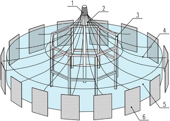
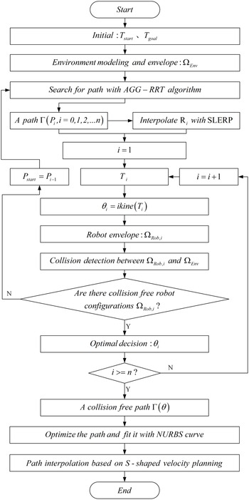
In this paper, robots are used in three-dimensional (3D) weaving equipment for large curved preforms of fiber composites, as shown in Fig. 1, where sixteen industrial robots mounted upside-down are distributed in a circle to perform synchronized yarn carding and yarn transfer. The robot motion paths are usually obtained by online manual calibration in practical engineering. However, it is laborious because there are many robot motion paths and the paths are not universal for different products. Furthermore, there are numerous robots and obstacles with limited space available for robots, so it is necessary to avoid collisions between neighboring robots and between robots and obstacles during robot motion, which further increases the difficulty of manually calibrating robot paths. Therefore, this paper proposes an obstacle avoidance path planning method for the simultaneous motion of multiple industrial robots to generate automatically optimal collision-free motion trajectories of robots, eliminating a lot of tedious manual calibration work and ensuring good motion performance of robot joints. The overall process of robot trajectory planning is shown in Fig. 2.
The sketch of weaving equipment. (Note that 1 is the woven preforms; 2 is the mandrel; 3 is the rack; 4 is elastic ropes; 5 is the movement space of robots; 6 is the unitary machine.).

The overall process of robot arm obstacle avoidance trajectory planning.

2. Search for robot end path
2.1. Basic RRT algorithm
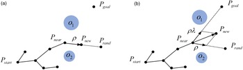
The building process of the Basic-RRT is shown in Fig. 3(a), where the blue circles are obstacles;
 $P_{\textit{start}}$
and
 $P_{goal}$
are the starting point and goal point, respectively;
 $P_{rand}\in \mathbb{R}$
is the random sampling point;
 $P_{near}$
is the nearest node to
 $P_{rand}$
in the random tree;
 $\rho$
is the step size for generating the new node
 $P_{new}$
.
Building process of the basic RRT (a) and the improved RRT (b).

2.2. AGG-RRT algorithm
To improve the search efficiency of the Basic-RRT algorithm, the improved RRT algorithm [Reference Cao, Zou, Jia, Chen and Zeng21] adding the goal-guided component was proposed, as shown in Fig. 3(b). The generation formula for extending the new node
 $P_{new}$
at node
 $P_{near}$
by the improved RRT algorithm follows.
 \begin{equation} P_{new}=P_{near}+\rho \cdot \frac{P_{rand}-P_{near}}{\left| P_{rand}-P_{near}\right| }+\rho \cdot \lambda \cdot \frac{P_{goal}-P_{near}}{\left| P_{goal}-P_{near}\right| } \end{equation}
In (1),
 $\lambda$
is the goal-guided factor. The goal-guided component guides the random tree to grow toward
 $P_{goal}$
, and the value of
 $\lambda$
determines its guidance ability. The larger the value of
 $\lambda$
, the stronger the guidance and the more concentrated the path. However, the obstacle avoidance ability is greatly limited. Search failures may occur if the search path encounters a sizeable spatial obstacle or goes through a narrow region because the random tree will oscillate around them. The smaller the value of
 $\lambda$
, the stronger the randomness, the more diffuse the path, and the stronger the obstacle avoidance ability, but this can not effectively shorten the search time. The improved RRT algorithm with a fixed goal-guided component cannot guarantee both good guidance ability and randomness at the same time, so its effect is poor when applied to a complex and changing environment. Therefore, this paper proposes the AGG-RRT algorithm, which adaptively and dynamically adjusts the value of
 $\lambda$
during the search process. When the path approaches obstacles, the value of
 $\lambda$
decreases to make it bypass the obstacle; when the path escapes from obstacles or approaches
 $P_{goal}$
, the value of
 $\lambda$
increases to enhance the guidance or slow down the oscillation phenomenon at the end of the path. The goal-guided factor
 $\lambda$
is defined as follows.
 \begin{equation}\lambda =\lambda _{max}\cdot e^{-\tau ^{\alpha }/{\varpi ^{\beta }}} \end{equation}
In (2):
 $\tau =\left| P_{near}-P_{goal}\right|$
is the goal estimated distance;
 $\varpi$
represents the minimum safe distance from
 $P_{near}$
to
 $P_{goal}$
, which is equal to the distance between
 $P_{near}$
and the obstacle nearest to
 $P_{near}$
and intersecting the line
 $\overline{P_{near}P_{goal}}$
minus the radius of that obstacle;
 $\alpha$
is the goal estimated distance factor;
 $\beta$
is the minimum safe distance factor;
 $\lambda _{max}$
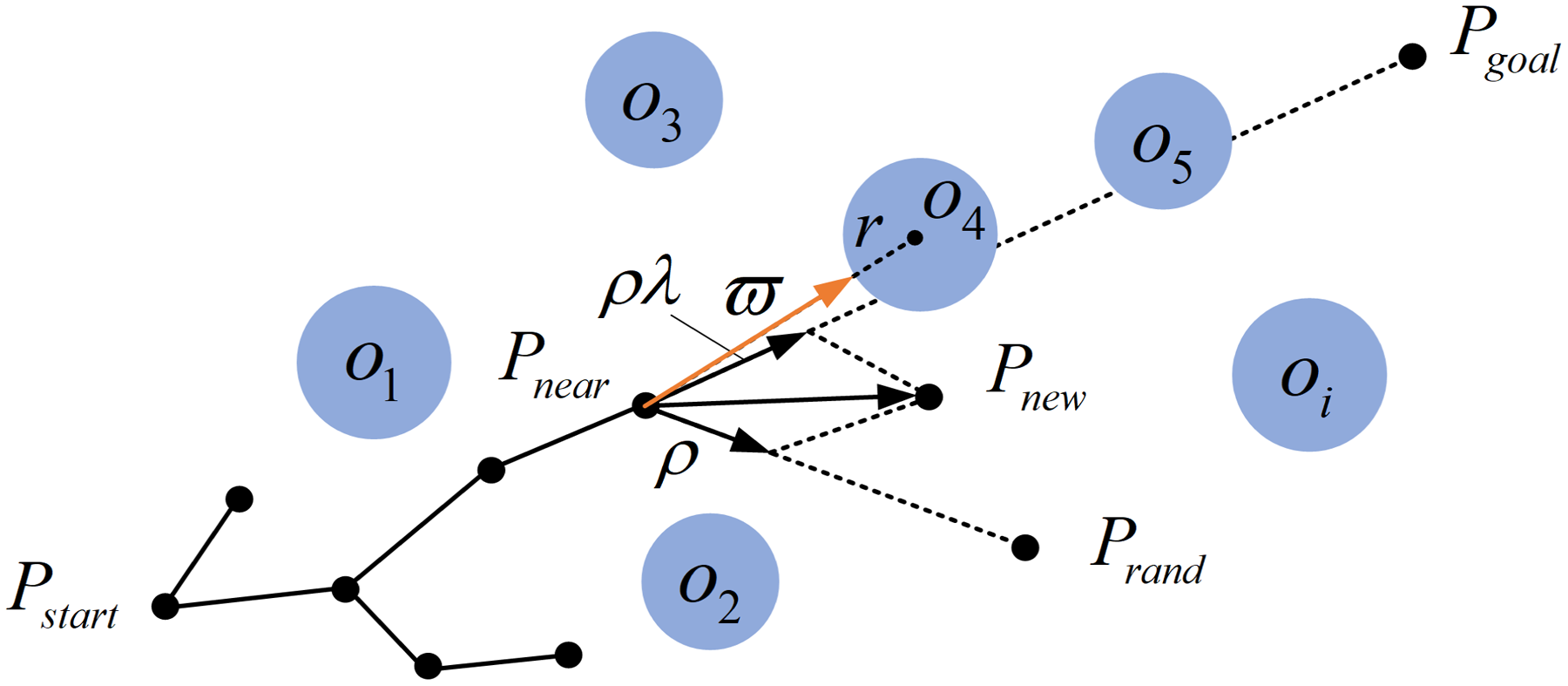
is the maximum value of the goal-guided factor. As shown in Fig. 4,
 $\left| P_{near}-o_{4}\right| -r$
is the minimum safe distance in the current situation.
Diagram of the minimum safe distance.

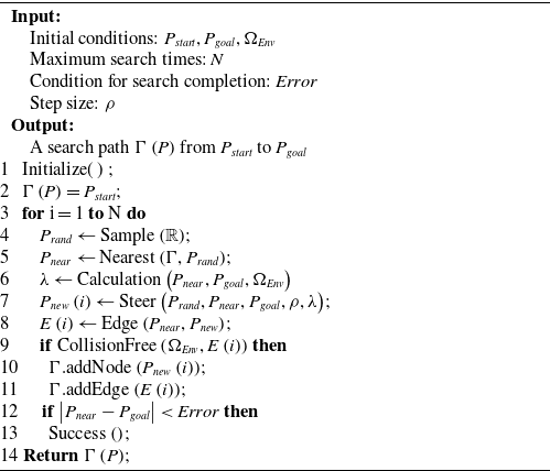
Algorithm 1 presents the pseudocode of the AGG-RRT algorithm. Where: ‘Calculation’ is the calculation function for
 $\lambda$
;
 $\Omega _{Env}$
represents the structure data that contains all the environment information.
AGG-RRT

3. Robot obstacle avoidance strategy in joint space
3.1. Orientation interpolation of the robot end
To obtain the joint coordinates of the robot by inverse kinematics, the orientation of each position needs to be interpolated after the positions of the collision-free path at the robot end are obtained by the AGG-RRT algorithm. There are three primary representations of the robot end orientation, namely, the Euler angle method, the rotation matrix method, and the quaternion method [Reference Dong, Yao, Li and Zhang25]. Among them, orientation interpolation based on the quaternion method is widely used because it has the advantages of avoiding the gimbal locking problem, simple operation, high efficiency, and smooth interpolation path [Reference Ahn, Chung and Jung26]. This section uses the spherical linear interpolation (SLERP) method based on unit quaternion to interpolate the orientation.
For any
 $R=\left[n_{x},o_{x},a_{x};n_{y},o_{y},a_{y};n_{z},o_{z},a_{z}\right]$
represented with the rotation matrix, it can be transformed into
 $q=q_{0}+q_{1}i+q_{2}j+q_{3}k\left(i^{2}=j^{2}=k^{2}=ijk=-1,{q_{0}}^{2}+{q_{1}}^{2}+{q_{2}}^{2}+{q_{3}}^{2}=1\right)$
represented with the unit quaternion by (3); conversely, the known
 $q$
can also be transformed into
 $R$
by (4).
 \begin{equation} \left[\begin{array}{l} q_{0}\\ \\[-7pt] q_{1}\\ \\[-7pt] q_{2}\\ \\[-7pt] q_{3} \end{array}\right]=\frac{1}{2}\left[\begin{array}{l} \sqrt{n_{x}+o_{y}+a_{z}+1}\\ \\[-4pt] sign\left(o_{z}-a_{y}\right)\sqrt{n_{x}-o_{y}-a_{z}+1}\\ \\[-4pt] sign\left(a_{x}-n_{z}\right)\sqrt{-n_{x}+o_{y}-a_{z}+1}\\ \\[-4pt] sign\left(n_{y}-o_{x}\right)\sqrt{-n_{x}-o_{y}+a_{z}+1} \end{array}\right] \end{equation}
 \begin{equation} R=\left[\begin{array}{c@{\quad}c@{\quad}c} {q_{0}}^{2}+{q_{1}}^{2}-{q_{2}}^{2}-{q_{3}}^{2} & 2\left(q_{1}q_{2}-q_{0}q_{3}\right) & 2\left(q_{1}q_{3}+q_{0}q_{2}\right)\\ \\[-7pt] 2\left(q_{1}q_{2}+q_{0}q_{3}\right) & {q_{0}}^{2}-{q_{1}}^{2}+{q_{2}}^{2}-{q_{3}}^{2} & 2\left(q_{2}q_{3}-q_{0}q_{1}\right)\\ \\[-7pt] 2\left(q_{1}q_{3}-q_{0}q_{2}\right) & 2\left(q_{2}q_{3}+q_{0}q_{1}\right) & {q_{0}}^{2}-{q_{1}}^{2}-{q_{2}}^{2}+{q_{3}}^{2} \end{array}\right] \end{equation}
The SLERP algorithm was proposed by Shoemake [27] in 1985 for equal rotation angle interpolation between two orientations, and the function of the SLERP algorithm is shown in (5).
 \begin{equation} \textit{SLERP}\left(q_{s},q_{e},t\right)=\frac{\sin \left(\left(1-t\right)w\right)}{\sin \left(w\right)}q_{s}+\frac{\sin \left(tw\right)}{\sin \left(w\right)}q_{e} \end{equation}
Where:
 $q_{s}$
and
 $q_{e}$
are the starting and terminal orientations, respectively;
 $w$
is the angle between
 $q_{s}$
and
 $q_{e}$
on the unit sphere, and
 $\cos \left(w\right)=q_{s}\cdot q_{e}$
;
 $t\in \left[0,1\right]$
.
3.2. Collision detection for the simultaneous motion of multi-robot
To simplify the operation and improve the response speed, the capsule and sphere bounding boxes [Reference Qin, Liu and Liu28] are first used to envelop the irregular robotic arm and the obstacles in the environment, achieving model simplification. The Euclidean distance between the bounding boxes is then used to evaluate the spatial occupancy relationship between the robotic arm and the obstacles, so the collision detection between robot and environment or between robot and robot is transformed into a simple geometry intersection detection problem. A collision is considered to have occurred if the minimum distance
 $d_{\min }$
between any two spheres or capsules minus the safety distance
 $\varepsilon$
is less than the sum of their radii.
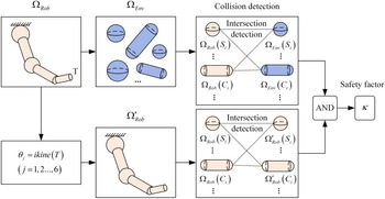
In this paper, sixteen robots with uniform circular distribution move synchronously, and it must be avoided that any of these robots collides with the obstacles in the environment or the adjacent robots during the motion. The collision detection process of a robot at position T is shown in Fig. 5. Firstly, the envelope model
 $\Omega _{Rob}$
of the robot and the envelope model
 $\Omega _{Env}$
of the environment are determined. Then, the joint coordinates
 $\theta$
of the robot are obtained, and the envelope model
 $\Omega '_{Rob}$
of the adjacent robot under the joint coordinates
 $\theta$
is obtained. Finally, collision detection is performed between the robot and the environment and between the robot and the adjacent robot, respectively. If no collision occurs, the robot is considered safe at the current position T, and the safety factor
 $\kappa =1$
is set; otherwise,
 $\kappa =0$
.
Schematic diagram of collision detection.

3.3. Optimal selection of robot joint coordinates
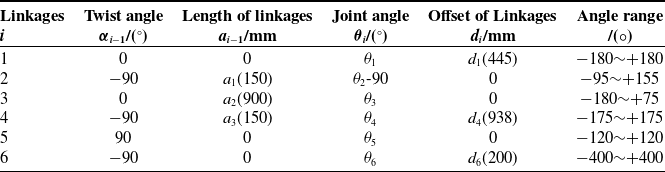
The robot studied in this paper is a 6-DOF industrial robot with model ABB-IRB2600ID_8_2. Its coordinate system is modeled with the Modified Denavit-Hartenberg (MD-H) method proposed by Khail and Kleinfinger [Reference Khalil and Kleinfinger29], and the MD-H parameters are shown in Table I. The axes of the rear three adjacent joints of this robot intersect at a point, satisfying the Pieper criterion [Reference Peiper30], so the closed-form solution of the inverse kinematics of this robot can be solved by the analytical method [Reference Zhou, Xian, Chen, Chen, Yang, Chen and Huang31]. For any robot end pose, there are theoretically eight sets of inverse kinematic solutions within
 $\theta _{i}\in \left(-\pi,\pi \right)\left(i=1,2,\ldots,6\right)$
, which reflect the eight spatial configurations of the robot arm. However, limited by the range of motion of each joint, there may be some unreachable solutions among them.
The MD-H parameters for the robot.

The optimal decision is required if there exist multiple configurations satisfying the collision-free condition(
 $\kappa =1$
). In practical applications, the optimal solution is usually selected based on the principles of minimum execution time, minimum energy consumption, minimum joint jerk, and so on [Reference Shi, Fang, Gang, Xu and Hua32]. An optimization function with the minimum sum of weighted rotational joint angles being the objective is proposed to meet the continuity of joint coordinate changes during robot motion. Different weights are assigned to each joint angle according to the different influence degree of each joint angle’s change on the robot’s end pose.
 \begin{equation} \Psi =\sum _{i=1}^{m}\sum _{j=1}^{n}w_{i}\left| \theta _{i,j+1}-\theta _{i,j}\right| \end{equation}
In (6):
 $\Psi$
is the minimum joint angle path optimization function; m is the number of the robot joints;
 $n+1$
is the number of the robot’s motion path points from the starting point to the goal point;
 $w_{i}$
is the weight coefficient of the i-th joint;
 $\theta _{i,j}$
is the rotation angle of the i-th joint at the j-th path point.
3.4. Correct the path in reverse
After obtaining the collision-free path
 $\Gamma$
of the robot end searched by the AGG-RRT algorithm, robot collision detection is performed in joint space, and the path is reverse corrected. The specific operation steps are as follows.
(1) Let
 $i=1$
.
(2) Let
 $i=i+1$
and assign the i-th point of the path
 $\Gamma$
to
 $P_{i}$
.
(3) Reverse solve for the eight sets of joint coordinates corresponding to the point
 $P_{i}$
; then perform collision detection for the robot’s space configuration under each set of joint coordinates in turn.
(4) If there are collision-free reachable configurations, the best joint coordinate is selected by optimal decision, and then go to (6); otherwise, (5) is performed.
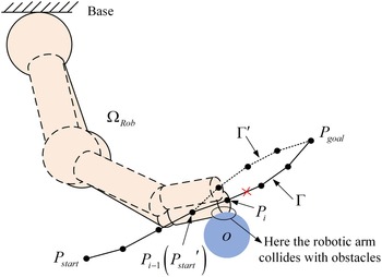
(5) As shown in Fig. 6, assuming that there is no collision-free configuration at the point
 $P_{i}$
, the path correction is performed as follows: (i) the path from
 $P_{i-1}$
, the previous point of
 $P_{i}$
, to the goal point is discarded; (ii)
 $P_{i-1}$
is considered as the new starting point
 ${P_{\textit{start}}}^{'}$
; (iii) the new path
 $\Gamma '$
is searched by AGG-RRT algorithm again; (iv) let
 $\Gamma =\left\{\Gamma \left(1,2,\ldots,i-2\right),\Gamma '\right\}$
.
The correction process of the collision-free path.

(6) Determine if
 $P_{i}=P_{goal}$
holds: if yes, a collision-free path
 $\Gamma \left(\theta \right)$
in joint space is generated and the task ends; otherwise, return to (2).
To prevent the corrected path from falling into local extremes and oscillating around the collision point
 $P_{i}$
, the randomness of the AGG-RRT algorithm in the initial state should be enhanced when the path is re-searched from
 $P_{i-1}$
. Therefore, the initial value of the goal-guided factor
 $\lambda$
is set to 0 so that the corrected path can avoid the region near
 $P_{i}$
.
4. Path optimization and velocity planning
4.1. Path optimization
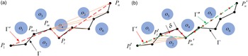
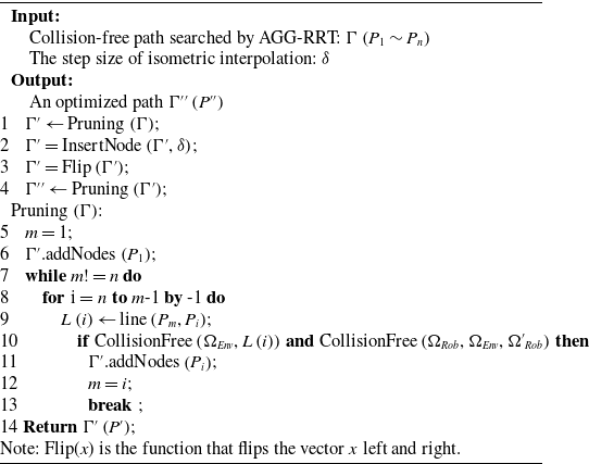
Since the AGG-RRT algorithm has certain randomness, the path generated by automatic search has some redundant nodes, increasing unnecessary path overhead. To shorten the length of the path and improve the efficiency of the robot, this section performs path optimization by pruning the redundant nodes of the path [Reference Wei and Ren17], which is shown in Fig. 7(a), and its specific steps are shown in lines 5 to 14 of pseudo-code Algorithm 2.
Bidirectional pruning of the path’s redundant nodes. (a) Forward; (b) Backward.

Most of the redundant nodes in the path can be removed by pruning forward. However, the method uses the idea of a greedy algorithm [Reference Bird and Mu33], which always looks for the farthest connectable collision-free point in the direction of the goal point, so the optimized path is not necessarily the globally optimal path. As in Fig. 7(a),
 $\Gamma '\left(P_{1}\rightarrow P_{m}\rightarrow P_{i}\rightarrow P_{n}\right)$
is the optimized path obtained by pruning forward, and obviously, there exists a path
 $P_{1}\rightarrow P_{m-1}\rightarrow P_{i}\rightarrow P_{n}$
with a shorter path length than it, so
 $\Gamma '$
is not the current optimal path. The path is further optimized by using secondary pruning backward in this section to solve this problem. As shown in Fig. 7(b), the forward-optimized path is interpolated isometrically with step size
 $\delta$
, and then the redundant nodes are backward pruned from the ending point. The backward pruning method is similar to forward pruning, and the second optimized path
 $\Gamma ''$
is finally obtained. The local optimization problem can be effectively overcome by bidirectional pruning. Algorithm 2 presents the pseudocode for bidirectional pruning of the redundant nodes.
Bidirectional pruning of the redundant nodes

4.2. NURBS curve fitting
The path still has folds and unsmoothness at the node connections after removing the redundant nodes, increasing the wear and tear of the robot and affecting its stability when it moves along this path. Therefore, the path is smoothed by using a cubic non-uniform rational B-spline (NURBS) curve with
 $C^{2}$
continuity in this paper. The k-th order NURBS curve is defined as follows [Reference Guo, Wu, Yang, Shen, Zhang, Zhang, Lou and Li34].
 \begin{equation} C\left(u\right)=\frac{\sum _{i=0}^{n}w_{i}d_{i}N_{i,k}\left(u\right)}{\sum _{i=0}^{n}w_{i}N_{i,k}\left(u\right)} \end{equation}
Where:
 $w_{i}\left(0\leq i\leq n;w_{0},w_{1}\gt 0;w_{i}\geq 0\right)$
is the weight factor, and the adjacent
 $k$
weight factors cannot be 0 simultaneously;
 $d_{i}\left(0\leq i\leq n\right)$
is the control vertex; node vector
 $U=\left[u_{0},u_{1},\ldots,u_{n+k+1}\right]$
(the overlap of nodes at both ends is
 $k+1$
);
 $N_{i,k}\left(u\right)$
is a k-th order norm B-spline basis function and satisfies the following definition.
 \begin{equation} \left\{\begin{array}{c} N_{i,k}\left(u\right)=\dfrac{u-u_{i}}{u_{i+k}-u_{i}}N_{i,k-1}\left(u\right)+\dfrac{u_{i+k+1}-u}{u_{i+k+1}-u_{i+1}}N_{i+1,k-1}\left(u\right)\\ \\[-7pt]N_{i,0}\left(u\right)=\left\{\begin{array}{l@{\quad}l} \begin{array}{l@{\quad}l} 1& if\,u_{i}\lt u\lt u_{i+1}\\ \\[-7pt]0&\textit{otherwise} \end{array} & u\in \left[0,1\right] \end{array}\right.\\ \\[-7pt]rule\colon \dfrac{0}{0}=0 \end{array}\right. \end{equation}
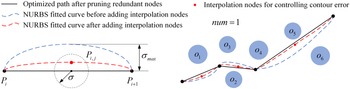
Whether the robot will collide with the obstacle during the motion along the path fitted by the NURBS curve is to be considered. Since the path before being fitted is completely collision-free, it can be transformed into the overlap problem of the path before and after being fitted by the NURBS curve. To improve the overlap of the fitted curve with the original path, it is necessary to interpolate more points on the original path, but this may lead to the result that the curvature value of the fitting curve at a certain point is tremendous even the fitting fails. Therefore, an interpolation method is designed to control the contour error of the fitted curve, obtaining a smooth curve while ensuring its high overlap with the original path.
As shown in Fig. 8, the interpolation formula for inserting num new nodes
 $P_{i,j}$
between every two adjacent points (
 $P_{i}$
and
 $P_{i+1}$
) is as follows.
 \begin{equation} P_{i,j}=P_{i}+j\cdot \left(P_{i+1}-P_{i}\right)/\left(num+1\right)+\textit{Randi}\left(\left[-1,1\right],1,D\right)\ast \sigma \end{equation}
Where:
 $\textit{Randi}\left(\left[-1,1\right],1,D\right)$
represents generating a D-dimensional coordinate in the range of [–1,1];
 $\sigma \left(\sigma \leq \sigma _{max}\right)$
is the parameter that controls the contour error of the fitted curve; the circle (2D space) or sphere (3D space) with a radius of
 $\sigma$
is the interpolation region of
 $P_{i,j}$
. The smaller the value of
 $\sigma$
or the larger the value of num, the higher the degree of overlap of the paths before and after the NURBS curve fitting. Therefore, setting the maximum contour error
 $\sigma _{max}$
smaller than the safe distance
 $\varepsilon$
of the collision detection can ensure that the robot will not collide with obstacles when moving along the path fitted by the NURBS curve.
Interpolation method to control the contour error of NURBS fitted curve.

4.3. Velocity planning of trajectory
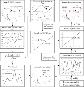
In the application of the NURBS curve on CNC machines, a constant feedrate profile will lead to large chord errors at the critical points with high curvature [Reference Liu, Huang, Yin, Guo, Shao and Zhang35]. Similarly, the speed of the robot end moving along the NURBS curve is limited by the curve’s curvature, and equal speed interpolation at points with large curvature causes large chord errors, so acceleration/deceleration planning is required at the extreme points of curvature. In this paper, the algorithm shown in Fig. 9 [Reference Xu, Zhang, Meng and Sun36] is used to achieve automatic interpolation of the final motion trajectory of the robot. The algorithm uses an S-shaped acceleration/deceleration planning, which can effectively reduce the chord errors of robot tracing motion and can mitigate the shock during acceleration/deceleration by constraining the maximum value of jerk, ensuring smooth movement of robot joints.
Automatic interpolation algorithm for the final motion trajectory of the robot.

5. Simulation experiments
5.1. AGG-RRT algorithm evaluation
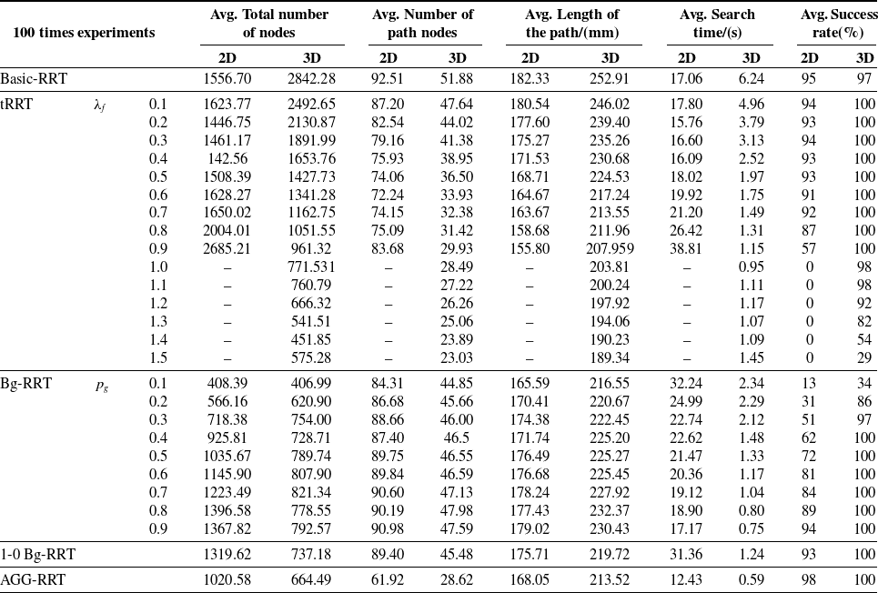
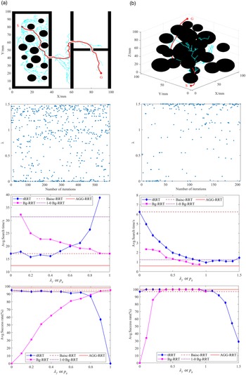
With S being the starting point and G being the target point, the Basic-RRT, tRRT, Bg-RRT, 1-0 Bg-RRT, and AGG-RRT are executed 100 times under the ‘DH’-shaped 2D map shown in Fig. 10(a) and the 3D map shown in Fig. 10(b), respectively. The terrain of the two maps is extremely complex, containing numerous obstacles, large obstacles, and narrow gaps. In this way, the performances of each algorithm in the complex environment are compared. The maximum number of iterations for each experiment is set to 10,000. The step size
 $\rho$
for all algorithms is 2 mm in the 2D map and 5 mm in the 3D map. The parameter
 $\lambda _{max}=1.5,\alpha =1,\beta =3$
in the AGG-RRT algorithm. Simulation results are shown in Table II, where
 $\lambda _{f}$
is the fixed goal-guided factor in tRRT, and
 $p_{g}$
is the probability of the goal point being selected as a random point in Bg-RRT.
Simulation comparison result of different algorithms.

Simulation results of the AGG-RRT algorithm and comparison with different algorithms. (a) 2D map; (b) 3D map.

From the simulation results in Table II and Fig. 10, the performance of the AGG-RRT algorithm has the following advantages over Basic-RRT, tRRT with different
 $\lambda _{f}$
, Bg-RRT with different
 $p_{g}$
, and 1-0 Bg-RRT in the complex environment.
(i)With the 2D map: the AGG-RRT algorithm has the shortest average search time of 12.43s; its average search path length is 168.05 mm, which is 7.83% shorter than the longest 182.33 mm (Basic-RRT), and 7.86% longer than the shortest 155.80 mm (tRRT with
 $\lambda _{f}=0.9$
); its average search success rate reaches 98%, which is the highest among all algorithms.
(ii)With the 3D map: the AGG-RRT algorithm has the shortest average search time of 0.59s; its average search path length is 213.52 mm, which is 15.57% shorter than the longest 252.91 mm (Basic-RRT), and 12.77% longer than the shortest 189.34 mm (tRRT with
 $\lambda _{f}=1.5$
); its average search success rate reaches 100%.
5.2. Path optimization and interpolation
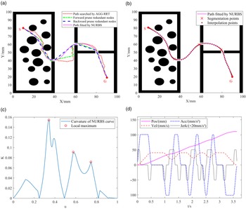
Taking the collision-free path automatically searched by AGG-RRT under the 2D map as an example, as shown in Fig. 11, the path optimization is firstly completed by bidirectional pruning of redundant nodes and fitted by the NURBS curve. Then the velocity planning is performed using the method in Section 4.3 to generate the final interpolated trajectory. Some parameters of velocity planning are set as follows: maximum velocity
 $v_{max}=40\ {\rm mm/s}$
; maximum acceleration
 $a_{max}=100\ {\rm mm/s}^{2}$
; maximum normal acceleration
 $a_{\textit{normal}}=50\ {\rm mm/s}^{2}$
; maximum jerk
 $J_{max}=1000\ {\rm mm/s}^{3}$
; maximum chord error
 $e_{max}=0.1\ {\rm mm}$
; interpolation period
 $\Delta T=0.02s$
.
Simulation results of path optimization and interpolation. (a) Redundant nodes pruning and NURBS fitting; (b) Path segmentation and interpolation; (c) Curvature of the NURBS fitted path; (d) S-shaped acceleration/deceleration planning.

5.3. Trajectory planning for multi-robot obstacle avoidance
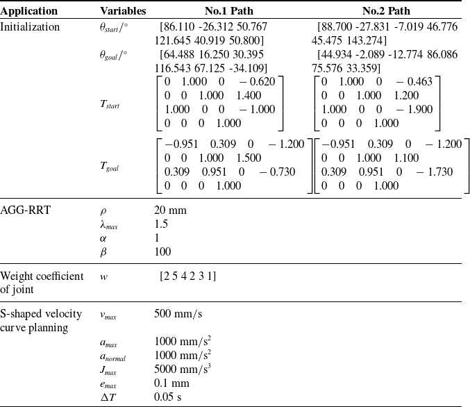
Firstly, the robots and obstacles are modeled for two adjacent units of the weaving equipment. Then, the robot’s obstacle avoidance path search and optimal trajectory planning are carried out under two working conditions, namely, the robot carrying yarn through the yarn winding device and the robot bypassing the yarn storage device, to verify the feasibility of the obstacle avoidance trajectory planning method for multi-robot simultaneous motion. The parameters of the simulation are shown in Table III.
Parameter data of the simulation.

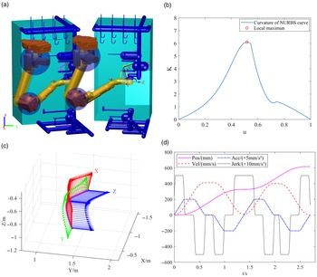
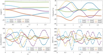
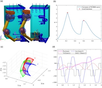
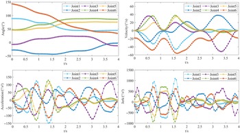
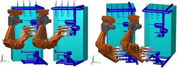
The simulation results of the two paths are shown in Figs. 12, 13, 14, 15 and 16. First, the collision-free paths are automatically searched and optimized, as shown in Figs. 12(a) and 14(a), where the yellow curves represent the collision-free paths automatically searched by the AGG-RRT algorithm; the black curves represent the paths optimized by bidirectional pruning redundant nodes; the red curves represent the paths fitted by NURBS curves. Then the NURBS fitted paths are segmented according to the local extrema of curve curvature shown in Figs. 12(b) and 14(b). Finally, the motion trajectories of the robot end are interpolated based on S-shaped acceleration/deceleration planning. The interpolated poses are shown in Figs. 12(c) and 14(c), and S-shaped acceleration/deceleration curves are shown in Figs. 12(d) and 14(d). The curves of robot joint motion are shown in Figs. 13 and 15, where the joint rotation angle curves, velocity curves, and acceleration curves are continuous and smooth, and the jerk curves are continuous. It indicates that the robot joint motion has good smoothness, and the impact and wear of the joints can effectively be reduced. As shown in Fig. 16, the two robots can automatically avoid obstacles, and they do not collide with each other when moving synchronously, indicating that the algorithm is effective and can plan the optimal motion trajectory.
Automatic search and optimal trajectory planning for No. 1 collision-free path.

Robot joint motion curve for No. 1 path.

Automatic search and optimal trajectory planning for No. 2 collision-free path.

Robot joint motion curve for No. 2 path.

The two robots move in sync to avoid obstacles.

6. Conclusion
In this paper, the following work is accomplished to solve the problem that it is difficult and laborious to calibrate obstacle avoidance paths in the skillful operation of multi-robots in 3D weaving equipment.
(i) An improved RRT algorithm (AGG-RRT) with adaptive goal guidance capability has been proposed. The simulation result demonstrates that the AGG-RRT algorithm has the shortest search time and the highest search success rate in the complex environment compared to some other improved RRT algorithms.
(ii) The AGG-RRT algorithm combined with the robot obstacle avoidance strategy is used to complete the automatic search of collision-free paths for multi-robot simultaneous motion. The path length is shortened by optimizing the path with the redundant points bidirectional pruning algorithm, and the path curve is fitted with a cubic NURBS curve to ensure the path curve is smooth.
(iii) With the extreme value of the path curve’s curvature being the constraint, the final motion trajectory of the robot is obtained by interpolation based on S-shaped acceleration/deceleration planning, avoiding excessive chord errors in the tracking motion of the robot and ensuring smooth motion of the robot joints.
Comprehensive simulation experiments have been conducted by the above method, showing that the proposed method is effective and has practical application value in the case of robots used for obstacle avoidance operations in the complex environment.
Author contributions
All authors contributed to the study conception and design; Material preparation, data collection, and analysis were performed by Xu Gaoping and Li Shuo; The first draft of the manuscript was written by Xu Gaoping and reviewed by Meng Zhuo; Resources were provided by Sun Yize; All authors read and approved the final manuscript.
Funding
This work was supported by Special Fund of Scientific and Technological Achievements Transformation in Jiangsu Province (BA2018061).
Competing interests
The authors have no relevant financial or non-financial interests to disclose.