1. Introduction
Access to high-resolution spatiotemporal flow fields is critical for a wide range of real-world applications, including the autonomous navigation of aerial and underwater vehicles (Lawrance & Sukkarieh Reference Lawrance and Sukkarieh2009; Masmitja et al. Reference Masmitja, Martin, O’Reilly, Kieft, Palomeras, Navarro and Katija2023; Zhang et al. Reference Zhang, Ji, Liu, Zhu and Xu2023), migration of microswimmers (Qiu et al. Reference Qiu, Mousavi, Gustavsson, Xu, Mehlig and Zhao2022a , Reference Qiu, Mousavi, Zhao and Gustavssonb ; Mousavi et al. Reference Mousavi, Qiu, Mehlig, Zhao and Gustavsson2024, Reference Mousavi, Qiu, Zhao, Mehlig and Gustavsson2025) and environmental monitoring (Smith Jr et al. Reference Smith, Sherman, McGill, Henthorn, Ferreira, Connolly and Huffard2021). For example, in unmanned aerial vehicles (UAVs) and underwater autonomous navigation, accurate knowledge of the underlying turbulent flow fields enables the implementation of globally optimal path planning algorithms including model predictive control (Krishna et al. Reference Krishna, Song and Brunton2022, Reference Krishna, Brunton and Song2023) and adaptive control (Landau et al. Reference Landau, Lozano, M’Saad and Karimi2011), which can outperform local decision-making approaches such as reinforcement learning (Reddy et al. Reference Reddy, Celani, Sejnowski and Vergassola2016, Reference Reddy, Wong-Ng, Celani, Sejnowski and Vergassola2018; Gunnarson et al. Reference Gunnarson, Mandralis, Novati, Koumoutsakos and Dabiri2021). This capability allows autonomous vehicles to identify and exploit beneficial flow features (e.g. updrafts), thereby improving energy efficiency and extending operational endurance. However, in realistic atmospheric or ocean environments, direct measurements of the full Eulerian flow field are often infeasible due to limited sensor coverage and the high cost of deployment. Instead, the available observation data are typically a single Lagrangian trajectory, collected by mobile sensors mounted on the vehicles themselves. These measurements are inherently Lagrangian in nature and often represent the only accessible data under operational conditions (Calascibetta et al. Reference Calascibetta, Biferale, Borra, Celani and Cencini2023; Jiao et al. Reference Jiao, Hang, Merel and Kanso2025). Several methods have been proposed to reconstruct Eulerian fields from Lagrangian observations. For example, FlowFit (Gesemann et al. Reference Gesemann, Huhn, Schanz and Schröder2016) and VIC+ (Schneiders & Scarano Reference Schneiders and Scarano2016) reconstruct Eulerian fields using physics-constrained approaches that achieve accurate reconstructions when dense particle tracking data are available. However, in realistic scenarios of autonomous aerial or underwater navigation, only a single Lagrangian trajectory may be accessible, and the information contained in such sparse measurements is insufficient for these methods. This situation poses a challenge: can we accurately reconstruct the flow field from a single Lagrangian trajectory?
This flow reconstruction challenge can be formulated as a super-resolution reconstruction problem, where the goal is to infer high-resolution flow fields from sparse and incomplete measurements. Conceptually, the task parallels classical image super-resolution in computer vision, where high-resolution images are reconstructed from their low-resolution counterparts (Wang, Zhou & Sun Reference Wang, Chen and Hoi2020c ). Given the sparsity of the available data, machine-learning-based super-resolution (MLSR) methods have emerged as promising tools to address this problem. Recent advances have extended MLSR methods to fluid flows by replacing the RGB (red, green and blue) image channels with physically meaningful quantities such as velocity or temperature fields (Fukami, Fukagata & Taira Reference Fukami, Fukagata and Taira2023). Building on this analogy, various machine learning architectures have been developed for flow-specific MLSR tasks. Fukami, Fukagata & Taira (Reference Fukami, Fukagata and Taira2019) introduced a convolutional neural network (CNN) architecture for a two-dimensional laminar cylinder wake and homogeneous decaying turbulence. Subsequent extensions include a spatiotemporal MLSR method (Fukami et al. Reference Fukami, Fukagata and Taira2021a ), a Voronoi tessellation-assisted MLSR method (Fukami et al. Reference Fukami, Maulik, Ramachandra, Fukagata and Taira2021b ) and a single-snapshot MLSR method (Fukami & Taira Reference Fukami and Taira2024), each tailored to distinct application scenarios. The applicability of MLSR approaches across diverse flow configurations has also been demonstrated by Liu et al. (Reference Liu, Tang, Huang and Lu2020), Nair & Goza (Reference Nair and Goza2020), Zhou et al. (Reference Zhou, McClure, Chen and Xiao2022) and Liu et al. (Reference Liu, Long, Wang, Chang and Qiu2026). To enhance the robustness and generalisability of these models, physics-informed loss functions that incorporate the governing equations of fluid dynamics have been introduced into the training process (Fukami et al. Reference Fukami, Fukagata and Taira2023). These physical constraints may be imposed in unsupervised learning (Bode et al. Reference Bode, Gauding, Lian, Denker, Davidovic, Kleinheinz, Jitsev and Pitsch2021; Gao, Sun & Wang Reference Gao, Sun and Wang2021) or incorporated as part of a hybrid loss function that combines physical consistency with a traditional mean square error loss function in supervised learning (Lee & You Reference Lee and You2019; Ren et al. Reference Ren, Rao, Liu, Ma, Wang, Wang and Sun2023). Recently, Weiss et al. (Reference Weiss, Emran, Bosbach and Shishkina2025) demonstrated an elegant physics-based method for reconstructing the temperature field by solving a Poisson equation derived from applying the curl operator twice to the Navier–Stokes equations. Similar to MLSR methods, this temperature field reconstruction requires Eulerian measurements.
Despite recent advancements, reconstructing flow fields from sparse Lagrangian trajectory data remains more challenging than conventional super-resolution tasks. First, the input measurements consist of irregularly sampled and temporally evolving trajectories. This irregularity hinders effective feature extraction by conventional CNN-based MLSR methods, thereby motivating the development of alternative architectures capable of directly processing Lagrangian inputs (Fukami et al. Reference Fukami, Fukagata and Taira2021b ). Second, in practical applications, trajectory data are often corrupted by sensor noise and localisation errors, which degrade signal quality and introduce uncertainties into the reconstructed flow fields. The reconstructions must remain physically consistent under such noisy conditions, particularly when gradient-related flow quantities (e.g. vorticity or velocity gradient) are of interest (Jiao et al. Reference Jiao, Hang, Merel and Kanso2025). These quantities are highly sensitive to even minor spatial errors in the reconstructed primitive fields, and any lack of physical consistency may result in significant distortions of the underlying flow structures.
Together, these challenges underscore the need for machine learning models that not only accommodate irregular and noisy Lagrangian trajectory data but also enforce physical consistency throughout the reconstruction process. In this work, we present a deep-learning model, termed track-to-flow (T2F), for reconstructing flow fields from the Lagrangian trajectories of self-propelling agents. The T2F model integrates a vision transformer (ViT) to capture spatiotemporal patterns within the trajectory data, and a CNN as the decoder to generate flow fields in the vicinity of the agent trajectories. In addition, a physics-informed loss function is incorporated to enhance the physical consistency, particularly in gradient-related quantities. The rest of this paper is organised as follows. In § 2, we introduce the T2F model in detail. In § 3, we validate the model in a laminar cylinder wake flow, serving as a proof-of-concept test. In § 4, we extend the application to turbulent Rayleigh–Bénard (RB) convection, a canonical flow system representative of convection in the atmosphere and oceans. The main findings of this work are summarised in § 5.
2. Numerical methods
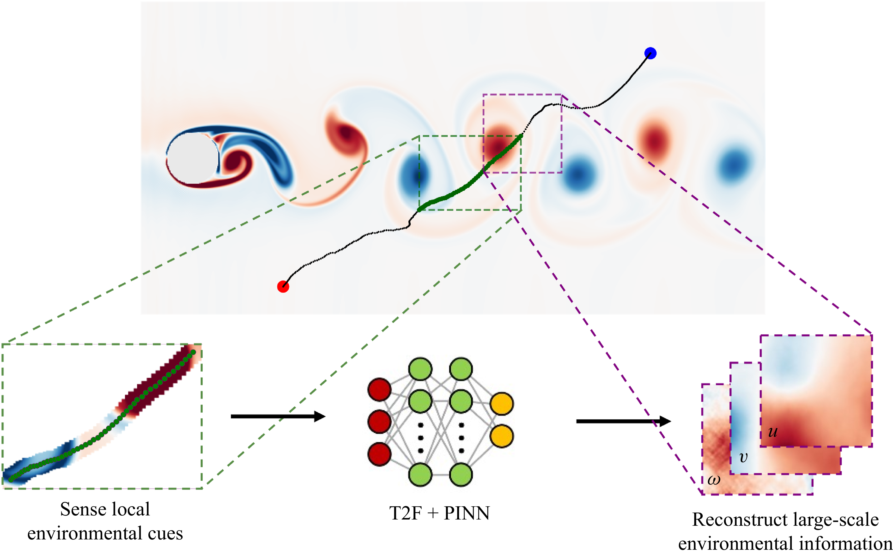
An overview of the T2F model is illustrated in figure 1. We first employ reinforcement learning to train self-propelling Lagrangian agents to perform point-to-point migration tasks within a flow environment, thereby generating agent trajectories as training data. Subsequently, the T2F model takes the trajectory information from the self-propelling agents as input and outputs the flow field in the vicinity of those trajectories.
Overview of the T2F model for reconstructing flow fields in the cylinder wake. An actively navigating Lagrangian agent collects local flow cues along its trajectory, which are subsequently used to infer the surrounding Eulerian flow field.
2.1. Migration of self-propelling agents
In this work, we consider an inertialess self-propelling agent model (Cichos et al. Reference Cichos, Gustavsson, Mehlig and Volpe2020), which is described as
 \begin{align} \boldsymbol{u}_{\textit{agent}} = \boldsymbol{u}_{\textit{fluid}} + \boldsymbol{u}_{\textit{propel}} &= \boldsymbol{u}_{\textit{fluid}} + U_{\textit{propel}} [\cos (\theta ), \sin (\theta )],\end{align}
 \begin{align} \boldsymbol{x}_{\textit{agent}}(t + {d}t)& = \boldsymbol{x}_{\textit{agent}}(t) + \boldsymbol{u}_{\textit{agent}}(t)\,dt ,\end{align}
where
 $dt$
is the time step. Here,
 $\boldsymbol{u}_{\textit{agent}}$
and
 $\boldsymbol{x}_{\textit{agent}}$
denote the velocity and position of the agent, respectively;
 $\boldsymbol{u}_{\textit{fluid}}$
is the local fluid velocity; and
 $U_{\textit{propel}}$
is the self-propelling velocity magnitude generated by the agent. The agent moves at a constant speed
 $U_{\textit{propel}}$
and directly controls its swimming direction
 $\theta$
. This is a toy model that describes the kinematics of UAVs in the atmosphere or autonomous underwater vehicles in the ocean. The model is justified by the fact that, in realistic atmospheric or oceanic scenarios, the characteristic length scale of the vehicles (of the order of metres) is several orders of magnitude smaller than that of the atmospheric or oceanic convection layer (typically kilometres). Similar dynamic models have been adopted in previous works (Biferale et al. Reference Biferale, Bonaccorso, Buzzicotti, Clark Di Leoni and Gustavsson2019; Borra et al. Reference Borra, Biferale, Cencini and Celani2022; Krishna, Song & Brunton Reference Krishna, Song and Brunton2022; Monthiller et al. Reference Monthiller, Loisy, Koehl, Favier and Eloy2022).
To control the migration behaviour of a self-propelling agent within a flow environment, we employ reinforcement learning, a model-free control strategy rooted in behavioural psychology, in which an agent learns optimal actions through trial-and-error interactions with its environment (Sutton & Barto Reference Sutton and Barto1998). Reinforcement learning has been increasingly applied in fluid mechanics, including drag reduction (Wang et al. Reference Wang, Wang, Zhou and Liu2022; Zhou, Zhang & Zhu Reference Zhou, Zhang and Zhu2025), heat transfer enhancement (Zhou & Zhu Reference Zhou and Zhu2025), vortex shedding control (Li & Zhang Reference Li and Zhang2022) and biologically inspired navigation tasks (Zhu, Fang & Zhu Reference Zhu, Fang and Zhu2022). In this work, we formulate a point-to-point migration problem, wherein agents are trained to reach randomly assigned target locations from randomly initialised starting points. The environmental cues available to the agent include its current position, its position relative to the target, the local fluid velocity and the target position. This information defines the observation state
 $s = [\boldsymbol{x}_{\textit{agent}}, \Delta \boldsymbol{x}_{\textit{agent}}, \boldsymbol{u}_{\textit{fluid}}, \boldsymbol{x}_{\textit{target}}]$
, where
 $\mathrm{\Delta } \boldsymbol{x}_{\textit{agent}} = \boldsymbol{x}_{\textit{target}} - \boldsymbol{x}_{\textit{agent}}$
. Based on this observation, the agent takes an action
 $a_t$
, defined as the control of the propulsion direction
 $\theta$
. The agent’s behaviour is shaped by a reward function that encourages efficient navigation towards the target. Following Gunnarson et al. (Reference Gunnarson, Mandralis, Novati, Koumoutsakos and Dabiri2021), we define the reward function as
 \begin{equation} r_t = -{dt} + 10\left [ \frac {\|\boldsymbol{x}_{t-1} - \boldsymbol{x}_{\textit{target}}\|}{U_{\textit{propel}}} - \frac {\|\boldsymbol{x}_t - \boldsymbol{x}_{\textit{target}}\|}{U_{\textit{propel}}} \right ] + r_{\textit{bonus}}, \end{equation}
where
 \begin{equation} r_{\textit{bonus}} = \begin{cases} 200, & \|\boldsymbol{x}_t - \boldsymbol{x}_{\textit{target}}\| \lt H/36\\[6pt] 0, & \text{others}. \end{cases} \end{equation}
Here,
 $\boldsymbol{x}_t$
and
 $\boldsymbol{x}_{t-1}$
denote the agent’s position at the current and previous time steps, respectively, and
 $H$
is the height of the computational domain. The first term of (2.3) penalises time consumption, thereby encouraging the agent to navigate quickly. The second term of (2.3) rewards progress towards the target, while the last term of (2.3) provides a large terminal reward for successful arrival within a defined proximity to the target.
The reinforcement learning training is conducted using the soft actor-critic algorithm, which aims to maximise both the expected cumulative reward (i.e. successful task completion) and the entropy of the policy (i.e. encouraging exploration). The optimisation objective is defined as
 \begin{equation} \pi ^{*}(\theta )=\arg \max _{\pi } E_{\tau \sim \pi }\left [ \sum _{t=0}^{\infty }\left \{ r_t(s_{t},a_{t},s_{t+1})+\alpha H[\pi (\boldsymbol{\cdot }| s_{t})] \right \} \right ]\!. \end{equation}
Here,
 $\pi$
denotes the policy, represented by a neural network that maps the observation state
 $s_t$
to a Gaussian distribution over actions
 $a_t$
. The notation
 $\pi (\boldsymbol{\cdot }| s_t)$
denotes that the policy is stochastic
 $\pi ^*$
denotes the optimal policy, i.e. the policy with optimised parameters
 $\phi ^*$
. The trajectory
 $\tau = (s_0, a_0, s_1, a_1, \ldots , s_t, a_t)$
represents a sequence of states and actions generated by the policy, and
 $\tau \sim \pi$
indicates that the trajectory is sampled from
 $\pi$
. The reward function is
 $r_t(s_t, a_t, s_{t+1})$
defined in (2.3), and
 $H[\pi (\boldsymbol{\cdot }| s_t)]$
is the entropy term that encourages exploration.
The entropy
 $H$
of the policy
 $\pi$
at state
 $s_t$
is computed as
 \begin{equation} H[\pi (\boldsymbol{\cdot }|s_{t})]=E_{a_t \sim \pi (\boldsymbol{\cdot }| s_{t})}[-\log \pi (a_t|s_{t})]. \end{equation}
For a Gaussian distribution
 $\pi (\boldsymbol{\cdot }| s_{t})$
over actions
 $a_t$
with mean
 $\mu (s_{t})$
and standard deviation
 $\sigma (s_{t})$
, the entropy can be simplified as
 \begin{equation} H[\pi (\boldsymbol{\cdot }| s_{t})] = \frac {1}{2} \log \big(2\pi e \sigma (s_{t})^2\big). \end{equation}
The entropy
 $H$
encourages exploration by favouring more stochastic policies. The parameter
 $\alpha$
is a trade-off coefficient that balances the reward and entropy terms. Further details of the soft actor-critic algorithm can be found in Haarnoja et al. (Reference Haarnoja, Zhou, Abbeel and Levine2018).
2.2. Deep-learning model: track-to-flow
We develop the T2F deep-learning model to reconstruct flow fields from the Lagrangian trajectories of self-propelling agents. The T2F model adopts an encoder–decoder architecture comprising a ViT as the encoder and a CNN as the decoder (see figure 2). Encoder–decoder architectures are widely employed in deep learning, particularly in natural language processing (Badrinarayanan, Kendall & Cipolla Reference Badrinarayanan, Kendall and Cipolla2017) and computer vision (Cho et al. Reference Cho, Van Merriënboer, Bahdanau and Bengio2014). The encoder transforms the input sequence into a set of high-dimensional feature representations, which are subsequently utilised by the decoder to generate the desired output. Such architectures have been successfully applied to aerodynamic feature extraction under extreme conditions (Fukami & Taira Reference Fukami and Taira2023).
Schematic of the T2F model architecture. The model consists of a ViT encoder that extracts spatiotemporal features from Lagrangian trajectory data, followed by a CNN decoder that reconstructs the corresponding Eulerian flow field.

In this study, the input to the model consists of localised trajectory data from self-propelling agents. These trajectories encode both fine-scale gradient information over short time scales and broader spatial–temporal correlations over longer horizons. Such multi-scale features are inherently difficult to extract using traditional methods. Interestingly, these input characteristics resemble those encountered in natural language processing and computer vision tasks, where close contextual relationships exist between adjacent words or pixels, while longer-range dependencies span across sentences or image regions. To this end, we adopt the Transformer architecture, which is capable of capturing both short- and long-range dependencies in sequential data. Specifically, we utilise the ViT as the encoder (Dosovitskiy et al. Reference Dosovitskiy2021), as illustrated on the left-hand side of figure 2. The ViT has demonstrated competitive performance in visual tasks by directly processing images as sequences of patches, which are small segments obtained by partitioning the input image. In the two-dimensional setting, we model a single particle trajectory as a short ‘video’ composed of local flow snapshots. The input of the T2F model encoder is a four-dimensional tensor
 $x_0 \in \mathbb{R}^{\,l_p \times l_p \times l_t \times C}$
, where
 $l_p$
is the edge length of each square patch so that one patch spans an
 $l_p \times l_p$
neighbourhood of grid points;
 $l_t$
is the number of time steps sampled along the trajectory; and
 $C$
denotes the number of physical channels stored at every grid point (e.g. the velocity components (
 $u$
,
 $v$
), pressure, temperature, etc.). Next, Transformer architecture is applied to extract spatiotemporal features from the Lagrangian input. The final output of the ViT encoder is a tensor
 $x_{\textit{ViT}}\in \mathbb{R}^{l_t \times d_e}$
, which represents a latent embedding of the input sequence.
Following feature extraction, a decoder is employed to reconstruct the corresponding Eulerian flow field. The decoder is based on a CNN, which is a class of deep-learning models widely used in image processing tasks (Li et al. Reference Li, Liu, Yang, Peng and Zhou2021). Through multiple layers of convolution and pooling, CNNs progressively extract and refine hierarchical spatial features. In this study, we utilise the inverse operation of convolution, namely deconvolution, to reconstruct the flow field from the encoded features. Specifically, the deconvolution operation transforms an input tensor
 $x_{\textit{in}} \in \mathbb{R}^{H_1\times W_1\times C_1}$
into an output tensor
 $ x_{\textit{out}} \in \mathbb{R}^{H_2\times W_2\times C_2}$
, as illustrated on the right-hand side of figure 2. The encoded features are first reshaped into multi-channel matrices and then progressively upsampled through multiple deconvolution layers. The final output is the reconstructed flow field
 $y \in \mathbb{R}^{H \times W \times C}$
, where
 $C$
represents the number of physical quantities being reconstructed and
 $H \times W$
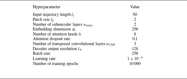
represents the spatial domain adjacent to the agent trajectories. Details of the T2F model architecture, including the number of layers and hyperparameters, are provided in Appendix A.
2.3. The physics-informed loss function
We employ a physics-informed loss function inspired by the framework of physics-informed neural networks (PINNs), which are a class of mesh-free methods for solving partial differential equations using neural networks (Raissi et al. Reference Raissi, Perdikaris and Karniadakis2019a ). In conventional neural network training, data-driven models learn mappings between inputs and outputs by minimising a loss function defined over labelled datasets. The PINNs extend this paradigm by incorporating governing physical laws (typically represented as differential equations) directly into the loss function. This approach enables the neural network to learn solutions that approximately satisfy the underlying physics, even in the absence of dense or high-fidelity training data. Although PINNs offer significant advantages, they enforce physical constraints only approximately, treating the governing equations as soft constraints. As a result, their accuracy may degrade when solving forward problems at moderate-to-high Reynolds numbers (Chuang & Barba Reference Chuang and Barba2022). Nevertheless, PINNs have demonstrated success in inverse problems, where system parameters or hidden fields must be inferred from sparse or noisy observations. Representative applications include the inference of structural properties, pressure and velocity fields (Raissi et al. Reference Raissi, Wang, Triantafyllou and Karniadakis2019b , Reference Raissi, Yazdani and Karniadakis2020; Boster, Cai & Ladr’o Reference Boster, Cai and Ladr’o2023), as well as the reconstruction of experimental flow velocity fields from noisy measurements (Cai et al. Reference Cai, Wang, Fuest, Jeon, Gray and Karniadakis2021; Kontogiannis et al. Reference Kontogiannis, Elgersma, Sederman and Juniper2022; Toscano et al. Reference Toscano, Käufer, Wang, Maxey, Cierpka and Karniadakis2025). It is worth mentioning that the philosophy of physics-informed approaches has also been applied to operators by embedding partial differential equations into the loss functions, such as a physics-informed neural operator, as Zhao et al. (Reference Zhao, Li, Fan, Wang, Yang and Wang2025) demonstrated in the novel application of LESnets (large-eddy simulation nets).
In the following, we first describe the mean-squared error loss function used in the standard T2F model, which does not incorporate any physics-based constraint. In the standard T2F model, the loss function
 $ L_{\textit{MSE}}$
is defined as
 \begin{equation} L_{\textit{T2F}} = L_{\textit{MSE}} = \frac {1}{N \times C} \sum _{j=1}^{C} \sum _{i=1}^{N} \big(y_{\textit{rec}}^{(i,j)} - y_{\textit{ref}}^{(i,j)}\big)^2 ,\end{equation}
where
 $N = H \times W$
is the total number of spatial grid points and
 $C$
is the number of physical quantities being reconstructed. The terms
 $y_{\textit{rec}}^{(i,j)}$
and
 $y_{\textit{ref}}^{(i,j)}$
denote the reconstructed value and the reference values, respectively, at the
 $i$
th grid point for the
 $j$
th physical quantity. Minimising this loss encourages the model to align its predictions closely with the ground-truth data.
To incorporate physical constraints, we augment the loss function with a physics-informed term, yielding the T2F+PINN model, in which the total loss function comprises a data loss
 $L_{\textit{MSE}}$
and an equation-based loss
 $L_{\textit{PDE}}$
. The equation loss is derived from the residual of the governing partial differential equations, expressed in general form as
 \begin{equation} \frac {\partial u}{\partial t} + \mathcal{N}[u] = 0, \quad x \in \varOmega , \, t \in [0,T], \end{equation}
where
 $ u(x,t)$
is the latent solution field,
 $ \mathcal{N}$
is a nonlinear differential operator,
 $ \varOmega$
is the spatial domain of the equation and
 $[0, T]$
is the time interval. The residual function is defined as
 \begin{equation} f = \frac {\partial u}{\partial t} + \mathcal{N}[u], \end{equation}
which quantifies the degree to which the reconstructed field violates the governing equations. The equation loss
 $ l_{\textit{PDE}}$
for a single equation is given by
 \begin{equation} l_{\textit{PDE}} = \frac {1}{N} \sum _{i=1}^{N} \left | f(t_i, y_i) \right |^2, \end{equation}
where
 $N$
is the number of grid points. Here,
 $f(t_i, y_i)$
denotes the residual evaluated at the
 $i$
th grid point, where
 $t_i$
is the time and
 $y_i$
is the reconstructed field value at that point. For systems governed by multiple equations, the total equation loss is a weighted sum of individual residuals:
 \begin{equation} L_{\textit{PDE}} = \sum _{k=1}^{N_{\!f}} w_k l_{\textit{PDE}}^k = \sum _{k=1}^{N_{\!f}} w_k \, \frac {1}{N} \sum _{i=1}^{N} \left | f_k(t_i, y_i) \right |^2, \end{equation}
where
 $N_{\!f}$
is the number of governing equations,
 $f_k$
denotes the residual for the
 $k$
th equation and
 $w_k$
is the corresponding weight. In summary, the full loss function for the physics-augmented T2F+PINN model is
 \begin{equation} L_{\textit{T2F+PINN}} = w_{\textit{data}} L_{\textit{MSE}} + \sum _{k=1}^{N_{\!f}} w_k \, l_{\textit{PDE}}^k ,\end{equation}
where
 $ w_{\textit{data}}$
and
 $ w_k$
control the relative contributions of data fidelity and physical consistency, respectively.
In this study, the inclusion of the physics-informed loss function transforms the reconstruction task into an inverse problem, in which the model aims to infer the latent Eulerian fields from observed Lagrangian trajectories. In contrast to conventional PINN formulations, the absolute spatial coordinates
 $\boldsymbol{x}$
and time
 $t$
are not supplied as explicit inputs to the network; instead, the model processes local Eulerian patches extracted along the particle trajectory, while spatiotemporal context is introduced only through learnable positional embeddings. As a result, we cannot apply automatic differentiation to compute temporal derivatives (e.g.
 $\partial u/\partial t,\ \partial T/\partial t$
). Instead, these temporal derivatives are calculated using the reference velocity and temperature fields obtained from numerical simulations. After training, we assess the reconstruction performance of both models using the normalised
 $L_2$
error, which provides a scale-invariant measure of accuracy. For a single reconstruction, the normalised
 $L_2$
error
 $\epsilon$
is defined as
 \begin{equation} \epsilon = \frac {\| y_{\textit{rec}} - y_{\textit{ref}} \|_2}{\| y_{\textit{ref}} \|_2}, \end{equation}
where
 $y_{\textit{rec}}$
and
 $y_{\textit{ref}}$
denote the reconstructed and reference fields, respectively, and
 $\lVert \boldsymbol{\cdot }\rVert _{2}$
is the Euclidean norm. This metric enables consistent comparisons across different datasets and physical quantities.
Trajectories of self-propelling agents navigating from the initial region (red) to the terminal region (blue) within the cylinder wake flow. The background contours represent the instantaneous out-of-plane vorticity field, illustrating the underlying flow structures guiding agent migration.

3. Flow field reconstruction in cylinder wake
3.1. Simulation settings
We evaluate the T2F and T2F+PINN models in a two-dimensional cylinder wake flow as a proof-of-concept test. The governing equations for the incompressible flow around a circular cylinder are
 \begin{align} \boldsymbol{\nabla }\boldsymbol{\cdot }\boldsymbol{u}& = 0,\end{align}
 \begin{align} \frac {\partial \boldsymbol{u}}{\partial t} + \boldsymbol{u} \boldsymbol{\cdot }\boldsymbol{\nabla \!}\boldsymbol{u} & = -\frac {1}{\rho }\boldsymbol{\nabla \!}p + \nu {\nabla} ^{2}\boldsymbol{u},\end{align}
where
 $\boldsymbol{u} = (u, v)$
is the velocity field,
 $\rho$
is the density,
 $p$
is the pressure and
 $\nu$
is the kinematic viscosity. To non-dimensionalise the equations, we introduce the following scaling:
 \begin{equation} \boldsymbol{x}^{\ast } = \frac {\boldsymbol{x}}{D}, \qquad t^{\ast } = \frac {t U_{\infty }}{D}, \qquad \boldsymbol{u}^{\ast } = \frac {\boldsymbol{u}}{U_{\infty }}, \qquad p^{\ast } = \frac {p}{\rho U_{\infty }^{2}}, \end{equation}
where
 $U_{\infty }$
is the free-stream velocity and
 $D$
is the cylinder diameter. The dimensionless governing equations then become
 \begin{align} \boldsymbol{\nabla }\boldsymbol{\cdot }\boldsymbol{u}^{\ast } & = 0,\end{align}
 \begin{align} \frac {\partial \boldsymbol{u}^{\ast }}{\partial t} + \boldsymbol{u}^{\ast } \boldsymbol{\cdot }\boldsymbol{\nabla \!}\boldsymbol{u}^{\ast }& = -\boldsymbol{\nabla \!}p^{\ast } + \frac {1}{\textit{Re}} {\nabla} ^{2}\boldsymbol{u}^{\ast }, \end{align}
where the Reynolds number is defined as
 \begin{equation} \textit{Re} = \frac {U_{\infty } D}{\nu }. \end{equation}
The computational domain is set to
 $[12D, 6D]$
and the mesh resolution is
 $1024 \times 512$
. The cylinder is placed at the centre of the domain at coordinates
 $(D, 3D)$
. The simulations are performed using the open-source lattice Boltzmann solver Palabos (Latt et al. Reference Latt2021) and are cross-validated with our in-house lattice Boltzmann solver (Xu & Li Reference Xu and Li2023, Reference Xu and Li2024). A Reynolds number of
 $\textit{Re} = 800$
is chosen. The resulting vorticity field exhibits a well-defined Kármán vortex street (see figure 3).
3.2. Migration of self-propelling agents
Using the simulated flow field, we train self-propelling agents via reinforcement learning to generate
 $n_{\textit{traj}} = 100$
point-to-point migration trajectories. As a benchmark, we refer to the study by Gunnarson et al. (Reference Gunnarson, Mandralis, Novati, Koumoutsakos and Dabiri2021). However, unlike their set-up, we modify the locations of the initial and terminal regions. In our configuration, agents migrate along the streamwise direction (see figure 3), whereas Gunnarson et al. (Reference Gunnarson, Mandralis, Novati, Koumoutsakos and Dabiri2021) reported zigzag-like trajectories aligned with the spanwise direction. This modification slightly reduces task complexity while significantly improving training efficiency. In our case, the agent’s reward signal saturates after approximately 1000 episodes and reaches its maximum value by around 4000 episodes. In contrast, the best-performing agent in the study of Gunnarson et al. required roughly 5000 episodes to plateau and more than 10 000 episodes to reach its optimal reward.
3.3. Evaluation of the T2F and T2F+PINN models
We evaluate the performance of the T2F and T2F+PINN models by reconstructing the velocity components in both the horizontal (
 $u_x$
) and vertical (
 $u_y$
) directions, corresponding to a total of
 $C = 2$
output channels. The reconstructed velocity fields are subsequently used to compute the out-of-plane vorticity, defined as
 $\omega _z = (\boldsymbol{\nabla }\times \boldsymbol{u})_{z}$
. The training dataset for both models is constructed as follows. First, the reinforcement learning agent described in § 3.2 is used to generate
 $n_{\textit{traj}} = 100$
point-to-point migration trajectories. From each trajectory,
 $n_{\textit{sample}} = 10$
segments are extracted at randomly chosen initial times, each segment consisting of 50 consecutive time steps. This yields a total of
 $n_{\textit{train}} = n_{\textit{traj}} \times n_{\textit{sample}} = 1000$
training samples. The same procedure is applied in the testing phase to generate
 $n_{\textit{test}} = 1000$
samples for evaluating the reconstruction accuracy of the models.
Figure 4 presents the reconstructed velocity fields obtained using the T2F and T2F+PINN models for a representative input, with the normalised
 $L_2$
error reported beneath each reconstructed flow field. We can see that both models are able to capture the spatial patterns of the flow structure. However, the reconstructions from the T2F model exhibit a noticeable blurring effect (see figure 4
d,e), resulting in the loss of fine-scale features. This blurring phenomenon is widely reported in flow-specific MLSR tasks across different flow scenarios (Fukami et al. Reference Fukami, Fukagata and Taira2019; Zhou et al. Reference Zhou, McClure, Chen and Xiao2022; Liu et al. Reference Liu, Ponce, Brunton and Kutz2023). In contrast, the T2F+PINN model occasionally produces spatial misalignments in the reconstructed flow structures (see figure 4
g,h). This raises a natural question: how do such visual discrepancies in the primitive flow variables (e.g. velocity) affect the accuracy of gradient-based quantities (e.g. vorticity)? When the reconstructed velocity field exhibits sharp but inconsistent transitions, as observed in the T2F model, the resulting vorticity computation becomes less accurate (see figure 4
f). This suggests that, although the purely data-driven T2F model can recover the overall flow structure, it lacks sufficient adherence to physical constraints necessary for accurately reconstructing gradient-based quantities. In contrast, the T2F+PINN model, by incorporating governing equations into the training process, effectively mitigates such inconsistencies and improves the accuracy of the reconstructed vorticity field (see figure 4
i). These differences underscore the importance of incorporating physics-informed constraints in enhancing the physical fidelity of reconstructions, particularly for gradient-related quantities. To illustrate the dynamic reconstruction process of the T2F model for the cylinder wake flow, the corresponding video can be viewed in supplementary movie 1 available at https://doi.org/10.1017/jfm.2025.11033.
Reconstruction results from the T2F and T2F+PINN models for a representative input in the cylinder wake. Ground-truth fields of (a) horizontal velocity
 $u_x^{\ast }$
, (b) vertical velocity
 $u_y^{\ast }$
and (c) out-of-plane vorticity
 $\omega _z^{\ast }$
. (d–f) Reconstructions by the T2F model. (g–i) Reconstructions by the T2F+PINN model. Listed values denote the normalised
 $L_2$
error
 $\epsilon$
.

Figure 5 shows the pointwise error fields associated with the reconstructions produced by the T2F and T2F+PINN models. For the T2F model, the reconstruction errors appear to be randomly distributed across the domain, with no discernible spatial structure (see figure 5 a–c). In contrast, the reconstruction errors from the T2F+PINN model exhibit geometrically structured patterns (see figure 5 d–f), indicating that the error distribution is more closely aligned with the underlying physical processes. In particular, the reconstructed vortical structures in the T2F+PINN case display physically constrained translations and deformations, rather than spurious or uncorrelated distortions. Compared with the results in figure 4, these observations suggest that incorporating physics-informed constraints via PINN leads to more accurate reconstructions of vortical structures, thereby improving the recovery of gradient-based flow features.
Pointwise reconstruction errors of the horizontal velocity
 $u_x^{\ast }$
, vertical velocity
 $u_y^{\ast }$
and vorticity
 $\omega _z^{\ast }$
in the cylinder wake: (a–c) the T2F model, (d–f) the T2F+PINN model.

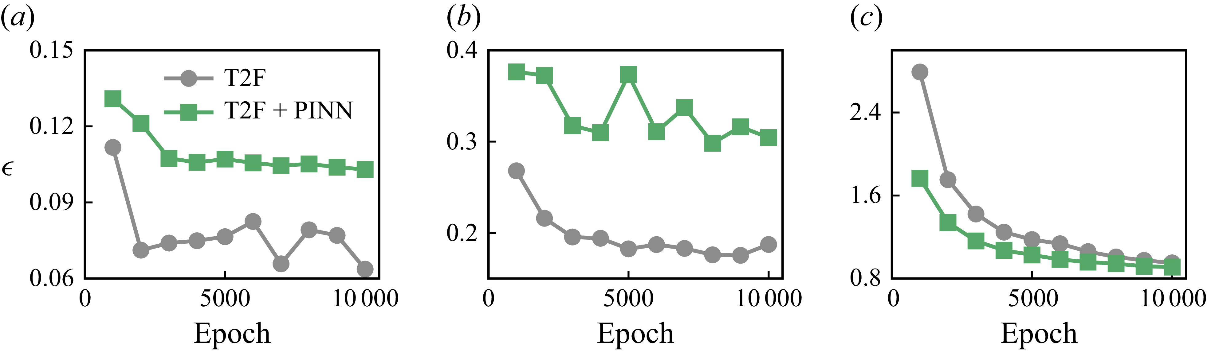
We also evaluated reconstruction errors across all
 $n_{\textit{test}} = 1000$
samples in the test set. Figure 6 shows the averaged normalised
 $L_{2}$
error for the reconstructed variables as a function of training epoch. For the T2F model, the errors in the reconstructed velocity component
 $u_x^{\ast }$
and
 $u_y^{\ast }$
at
 $10\,000$
training epochs are approximately 0.06 and 0.19, respectively, which are much lower than those of the T2F+PINN model (see figure 6
a,b), corresponding to reductions of approximately 38.1 % and 38.4 %. In contrast, the vorticity error of the T2F+PINN model at
 $10\,000$
epochs is approximately 0.91, slightly lower than that of the T2F model, with a reduction of around 4.2 % (see figure 6
c). These differences reflect the learning behaviours of the two models. The purely data-driven T2F model rapidly captures the dominant velocity structures but struggles to learn accurate velocity gradients, leading to higher errors in vorticity. The T2F+PINN model, on the other hand, incorporates physics-based constraints via the governing equations. While this results in a modest degradation in velocity reconstruction compared with the T2F model, it significantly enhances the fidelity of the reconstructed vorticity field. Similar trends have been reported by Yousif, Yu & Lim (Reference Yousif, Yu and Lim2021), who observed that optimisation using only data loss produced distorted fluctuations in velocity components, whereas incorporating physics-based loss reduced sharpness in the flow-field details. We attribute this trade-off to the inherently multi-objective nature of the T2F+PINN framework. In addition to the data loss minimised by the single-objective T2F model, it introduces a physics-based loss term (see § 2.3). During training, these competing objectives require compromise, forcing the T2F+PINN model to balance physical consistency against direct data fidelity. As a result, when evaluated purely in terms of data loss (i.e. the
 $L_{2}$
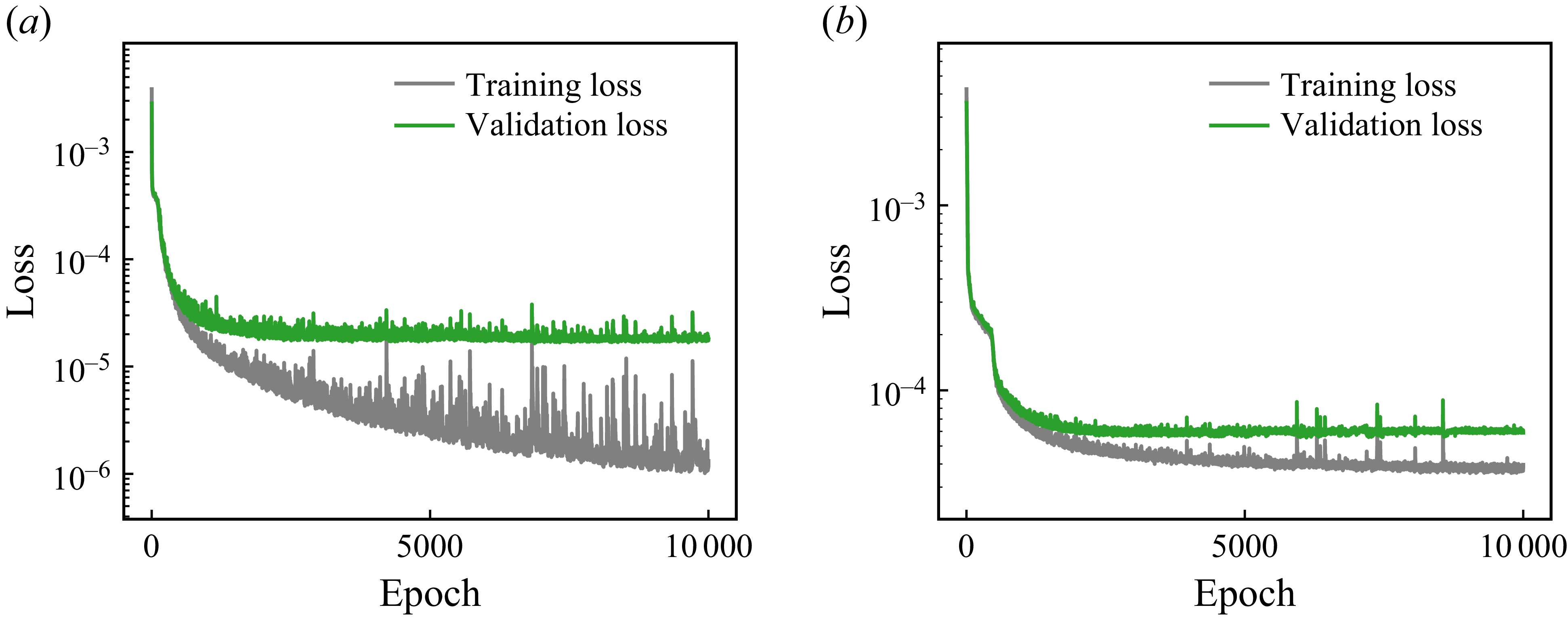
error for primitive variables), the T2F+PINN model may underperform relative to the T2F model. It is noteworthy that the fluctuations observed in figure 6(a,b) reflect variations in test-set performance, rather than instability in the training process. Instead, training convergence is confirmed by monitoring the loss on a small held-out validation set during training. To demonstrate that the model has reached convergence, the corresponding training and validation loss curves are provided in Appendix B.
Evolution of the normalised
 $L_{2}$
errors over training epochs for the cylinder wake reconstruction task. Reconstruction errors for (a) horizontal velocity
 $u_x^{\ast }$
, (b) vertical velocity
 $u_y^{\ast }$
and (c) vorticity
 $\omega _z^{\ast }$
, comparing the performance of the T2F and T2F+PINN models.

To benchmark our method, we compare its performance with that of the MLSR approach by Fukami et al. (Reference Fukami, Fukagata and Taira2019), which reconstructs high-resolution Eulerian fields from downsampled Eulerian inputs. Although the problem settings differ substantially, as our model infers flow fields from sparse Lagrangian trajectories, whereas Fukami et al. (Reference Fukami, Fukagata and Taira2019) reconstruct high-resolution fields from uniformly downsampled low-resolution data, we think such a comparison is still informative in interpreting the achievable reconstruction error levels. In the study by Fukami et al. (Reference Fukami, Fukagata and Taira2019), a normalised
 $L_2$
error of approximately
 $\epsilon = 0.04$
was reported, when reconstructing a
 $192 \times 112$
high-resolution field from a
 $12 \times 7$
low-resolution input using 1000 snapshots. In comparison, our T2F model was also trained on 1000 samples, and it achieves a normalised
 $L_2$
error of approximately
 $\epsilon = 0.06$
when reconstructing a
 $128 \times 128$
velocity field from
 $2 \times 2 \times 50$
trajectory-based measurements. This similarity in error magnitude demonstrates the data efficiency of our proposed T2F model, particularly considering its reliance on sparse, irregular and non-grid-aligned Lagrangian inputs.
In this work, we model an unmanned aerial or underwater vehicle as a point-particle agent. In practice, however, such vehicles have finite size and often carry multiple sensors, making it reasonable to assume that local flow information in the vicinity of the particle is accessible. Accordingly, in our simulations each temporal slice of the trajectory corresponds not to a single-point measurement, but to a square spatial patch of size
 $l_p \times l_p$
centred on the particle position, containing
 $C$
physical variables (
 $C = 2$
for
 $u$
,
 $v$
). We investigate the robustness of the T2F and T2F+PINN models under varying patch size
 $l_p$
. We consider four patch sizes:
 $l_p = 1$
,
 $2$
,
 $4$
and
 $8$
grid points. For
 $l_p = 1$
, the input patch is a single point, which represents the limiting scenario in which the particle probes only a single point per time step, and it is obtained by bilinear interpolation of the nearest grid point. The results averaged over
 $n_{\textit{test}}=1000$
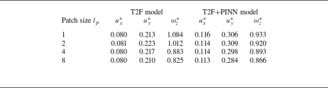
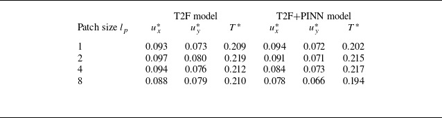
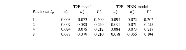
test samples and six independent simulations for T2F and T2F+PINN model are shown in table 1. For the cases
 $l_p=1$
and
 $l_p=2$
(corresponding to typical UAV scenarios with one or four sensors), the T2F model is more accurate for reconstructing the primary flow variables (e.g. velocity components
 $u_x^*$
and
 $u_y^*$
), whereas the T2F+PINN model has an advantage in reconstructing gradient-related quantities (e.g. vorticity
 $\omega _z^*$
). For larger patch sizes
 $l_p=4$
and
 $l_p=8$
(corresponding to UAV scenarios with 16 or 64 sensors), the T2F model outperforms the T2F+PINN model for all variables. We attribute this behaviour to the increased information content available by larger patch sizes, which reduces the relative impact of the PINN constraints. Moreover, for both models, the reconstruction errors for
 $u_x^{\ast }$
and
 $u_y^{\ast }$
remain relatively stable across different patch sizes, with a maximum variation of about 5 %. The vorticity error
 $\omega _z^{\ast }$
exhibits a slightly larger variation of about 14 % when the patch size is increased from
 $l_p = 1$
to
 $l_p = 8$
. Overall, the T2F and T2F+PINN models demonstrate robust performance across a range of patch sizes, indicating their flexibility in handling different spatial scales of input data.
Normalised
 $L_2$
errors of the reconstructed velocity components and vorticity fields in the cylinder wake for different patch sizes
 $l_p$
. The results are averaged over
 $n_{\textit{test}}=1000$
test samples and six independent simulations.

Reconstruction results of the T2F model under varying levels of input noise for a representative test sample: (a–c) horizontal velocity
 $u_x^{\ast }$
, vertical velocity
 $u_y^{\ast }$
and vorticity
 $\omega _z^{\ast }$
at a noise level of
 $\eta = 0.1$
; (d–f) reconstructions at
 $\eta = 0.2$
; and (g–i) reconstructions at
 $\eta = 0.5$
. Listed values denote the
 $L_2$
error
 $\epsilon$
.

In practical applications, observed environment cues may be contaminated by noise arising from sensor inaccuracies or environmental disturbances. To further evaluate the robustness of our model, we assess the performance of the T2F and T2F+PINN models under varying levels of input noise. Specifically, Gaussian noise is added to the input variable in the test set, which consists of the two velocity components
 $(u_x, u_y)$
. For each component, random values are drawn independently from a normal distribution
 $\mathcal{N}(x_{\textit{mean}}, x_{\textit{max}}/3)$
, where
 $x_{\textit{mean}}$
and
 $x_{\textit{max}}$
denote the mean and maximum values of that component, respectively. This design choice reflects realistic scenarios in autonomous aerial or underwater navigation, where onboard sensors measure local velocities, and adding noise to the measured variables therefore provides a faithful representation of sensor uncertainty. The noisy input is given by
 \begin{equation} x_{\textit{noise}} = x_{\textit{input}} + \eta \boldsymbol{\cdot }\mathcal{N}(x_{\textit{mean}}, x_{\textit{max}}/3), \end{equation}
where
 $\eta$
controls the noise amplitude. We consider three noise levels of
 $\eta = 0.1$
,
 $0.2$
and
 $0.5$
. Figures 7 and 8 present the reconstructed velocity components
 $u_x^{\ast }$
,
 $u_y^{\ast }$
and the vorticity
 $\omega _z^{\ast }$
obtained from the T2F and T2F+PINN models, respectively, for a representative test case under each noise level. At the low noise level (
 $\eta = 0.1$
), the T2F+PINN model achieves lower reconstruction errors in
 $u_x^{\ast }$
(0.080 versus 0.097) and
 $\omega _z^{\ast }$
(0.613 versus 0.819), while yielding a slightly higher error in
 $u_y^{\ast }$
compared with the T2F model (see figures 7
a–c and 8
a–c). As the noise level increases to
 $\eta = 0.2$
, the T2F model experiences substantial degradation in velocity reconstruction, with relative error increases of 85.6 % for
 $u_x^{\ast }$
and 146 % for
 $u_y^{\ast }$
. In contrast, the T2F+PINN model exhibits improved robustness, with smaller error increases of 65.0 % and 42.1 % for
 $u_x^{\ast }$
and
 $u_y^{\ast }$
, respectively. For the vorticity field, the T2F+PINN model shows only a 14.0 % increase in error, compared with a 28.0 % increase for the T2F model (see figures 7
d–f and 8
d–f). Under high noise levels (
 $\eta = 0.5$
), both models fail to reconstruct coherent vortex structures, with large errors across all fields. Nevertheless, the T2F+PINN model continues to yield relatively lower errors in
 $\omega _z^{\ast }$
, reflecting its superior resilience to noise (see figures 7
g–i and 8
g–i). In summary, as noise levels increase, the T2F model exhibits a significant decrease in reconstruction accuracy, especially for vorticity, whereas the T2F+PINN model maintains more stable performance across a wide range of noise levels.
Reconstruction results of the T2F+PINN model under the same input noise levels as in figure 7: (a–c) horizontal velocity
 $u_x^{\ast }$
, vertical velocity
 $u_y^{\ast }$
and vorticity
 $\omega _z^{\ast }$
at a noise level of
 $\eta = 0.1$
; (d–f) reconstructions at
 $\eta = 0.2$
; and (g–i) reconstructions at
 $\eta = 0.5$
. Listed values denote the
 $L_2$
error
 $\epsilon$
.

Normalised
 $L_{2}$
errors
 $\epsilon$
of the reconstructed (a)
 $u_x^{\ast }$
, (b)
 $u_y^{\ast }$
and (c)
 $\omega _z^{\ast }$
as functions of input noise levels
 $\eta$
, for the T2F and T2F+PINN models in the cylinder wake.

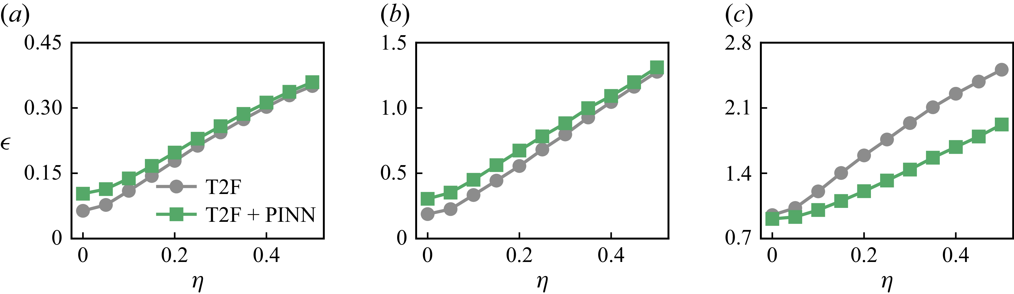
We further assess the influence of input noise on the T2F and T2F+PINN models by computing the average reconstruction error over the entire test set consisting of
 $n_{\textit{test}} = 1000$
samples. Figure 9 presents the variation of the normalised
 $L_{2}$
error
 $\epsilon$
with respect to the noise amplitude
 $\eta$
for the velocity components
 $u_x^{\ast }$
and
 $u_y^{\ast }$
as well as the vorticity
 $\omega _z^{\ast }$
. As shown in figure 9(a,b), the T2F model exhibits slightly lower reconstruction errors for
 $u_x^{\ast }$
and
 $u_y^{\ast }$
at low noise levels (
 $\eta \lt 0.1$
). However, its performance degrades more rapidly as noise increases, resulting in error levels comparable to those of the T2F+PINN model at higher noise (
 $\eta = 0.5$
). In contrast, the T2F+PINN model displays a more gradual increase in error, demonstrating enhanced robustness in reconstructing primitive variables under noisy input conditions. For the vorticity field (figure 9
c), the T2F+PINN model consistently outperforms the T2F model across all noise levels. Its error increases at a slower rate, indicating that the incorporation of physics-based constraints via the PINN framework effectively mitigates the degradation in gradient-based quantities caused by input noise. These findings confirm that although both models are affected by noise in the input trajectories, the T2F+PINN model exhibits superior robustness, particularly in reconstructing derived flow features such as vorticity. Similar robustness of physics-informed loss function has also been demonstrated in classical flow-specific MLSR tasks (Fukami et al. Reference Fukami, Fukagata and Taira2023).
4. Flow field reconstruction in Rayleigh–Bénard convection
4.1. Simulation settings
The RB convection is a canonical system for modelling buoyancy-driven flows in the atmosphere and oceans (Lohse & Xia Reference Lohse and Xia2010; Chillà & Schumacher Reference Chillà and Schumacher2012; Xia Reference Xia2013; Wang et al. Reference Wang, Zhou and Sun2020a ; Lohse & Shishkina Reference Lohse and Shishkina2023, Reference Lohse and Shishkina2024; Xia et al. Reference Xia, Huang, Xie and Zhang2023, Reference Xia, Chong, Ding and Zhang2025). In RB convection, thermal plumes emerge from the thermal boundary layers near the hot and cold walls and subsequently interact to form a coherent large-scale circulation structure. We simulate RB convection under the Oberbeck–Boussinesq approximation, wherein temperature is treated as an active scalar that modulates the velocity field via a buoyancy force. The governing equations for the RB convection system are given by
 \begin{align} \boldsymbol{\nabla }\boldsymbol{\cdot }\boldsymbol{u}& = 0,\end{align}
 \begin{align} \frac {\partial \boldsymbol{u}}{\partial t} + \boldsymbol{u} \boldsymbol{\cdot }\boldsymbol{\nabla \!}\boldsymbol{u}& = -\frac {1}{\rho _0}\boldsymbol{\nabla \!}P + \nu {\nabla} ^{2}\boldsymbol{u} + g\beta _T(T - T_0)\hat {\boldsymbol{y}},\end{align}
 \begin{align} \frac {\partial T}{\partial t} + \boldsymbol{u} \boldsymbol{\cdot }\boldsymbol{\nabla \!}T & = \alpha _T {\nabla} ^{2} T,\end{align}
where
 $\boldsymbol{u} = (u, v)$
,
 $P$
and
 $T$
denote the velocity, pressure and temperature fields, respectively;
 $\rho _0$
and
 $T_0$
are the reference density and temperature, respectively;
 $\hat {\boldsymbol{y}}$
is the unit vector in the direction of gravity;
 $g$
is the gravitational acceleration; and
 $\nu$
,
 $\beta _T$
and
 $\alpha _T$
represent the kinematic viscosity, thermal expansion coefficient and thermal diffusivity, respectively. With the following scaling:
 \begin{align} \boldsymbol{x}^{\ast }& = \frac {\boldsymbol{x}}{H}, \qquad t^{\ast } = \frac {t}{\sqrt {H/ (g\beta _{T}\!\varDelta _{T})}}, \qquad \boldsymbol{u}^{\ast } = \frac {\boldsymbol{u}}{\sqrt {g\beta _{T}\!H\! \varDelta _{T}}},\end{align}
 \begin{align} P^{\ast }& = \frac {P}{\rho _{0} g \beta _{T}\!\varDelta _{T}\! H}, \qquad T^{\ast } = \frac {T - T_{0}}{\varDelta _{T}},\end{align}
the governing equations can then be rewritten in dimensionless form as
 \begin{align} \boldsymbol{\nabla }\boldsymbol{\cdot }\boldsymbol{u}^{\ast }& = 0,\end{align}
 \begin{align} \frac {\partial \boldsymbol{u}^{\ast }}{\partial t^{\ast }} + \boldsymbol{u}^{\ast } \boldsymbol{\cdot }\boldsymbol{\nabla \!}\boldsymbol{u}^{\ast } & = -\boldsymbol{\nabla \!}P^{\ast } + \sqrt {\frac {\textit{Pr}}{Ra}}{\nabla} ^{2}\boldsymbol{u}^{\ast } + T^{\ast }\hat {\boldsymbol{y}},\end{align}
 \begin{align} \frac {\partial T^{\ast }}{\partial t^{\ast }} + \boldsymbol{u}^{\ast } \boldsymbol{\cdot }\boldsymbol{\nabla \!}T^{\ast }& = \sqrt {\frac {1}{\textit{Pr}\,Ra}}{\nabla} ^{2}T^{\ast }.\end{align}
Here
 $H$
is the cell height and it is chosen as the characteristic length;
 $t_{f} = \sqrt {H/(g\beta _{T}\!\varDelta _{T})}$
is the free-fall time and it is chosen as the characteristic time;
 $T_{0}$
is the temperature of the cooling walls; and
 $\varDelta _{T}$
is the temperature difference between the heating and cooling walls. The system is characterised by two dimensionless numbers, the Rayleigh number (
 $Ra$
) and the Prandtl number (
 $\textit{Pr}$
), defined as
 \begin{equation} Ra = \frac {g\beta _{T}\!\varDelta _{T}\!H^{3}}{\nu \alpha _{T}}, \qquad \textit{Pr} = \frac {\nu }{\alpha _{T}}. \end{equation}
Trajectories of agents navigating from the initial region (red) to the terminal region (blue) in RB convection. The background contours show the instantaneous temperature field, highlighting thermal plumes and large-scale circulation structures.

We employ the finite-volume solver OpenFOAM (Weller et al. Reference Weller, Tabor, Jasak and Fureby1998) and cross-validate the results against our in-house lattice Boltzmann solver (Xu & Li Reference Xu and Li2023, Reference Xu and Li2024) for RB convection at Rayleigh number
 $Ra = 10^{8}$
and Prandtl number
 $\textit{Pr} = 0.71$
. The computational domain is set to
 $[2H, H]$
, corresponding to an aspect ratio
 $\varGamma = 2$
. The domain is discretised using a uniform grid with a resolution of
 $1024 \times 512$
. The simulation was carried out for a total of 200 free-fall times with an adaptive time step ensuring the Courant–Friedrichs–Lewy number
 $\leq 0.3$
. To eliminate transient effects, the initial 167 free-fall times were discarded as spin-up. Subsequently, snapshots were recorded every 0.01 free-fall times. For training and testing, we used 1000 frames, corresponding to the statistically stationary interval between 167 and 177 free-fall times. A representative snapshot of the temperature field is shown in figure 10, where thermal plumes emerging from the top and bottom boundaries are clearly visible. These plumes self-organise into two oppositely rotating large-scale circulations, characteristic of RB convection at this parameter regime (Lohse & Shishkina Reference Lohse and Shishkina2023, Reference Lohse and Shishkina2024; Shishkina & Lohse Reference Shishkina and Lohse2024).
4.2. Migration of self-propelling agents
Using the simulated flow field, we trained the self-propelling agents via reinforcement learning to generate
 $n_{\textit{traj}} = 100$
trajectories, following the same navigation protocol as described in the cylinder wake case (see § 3). The resulting trajectories are shown in figure 10. Agents are initialised in a designated region near the lower-left corner of the domain. They are initialised, advected upward by the ascending hot plumes, traverse the bulk of the convection cell and subsequently descend along the cold plumes near the cell centre, eventually accumulating in a terminal region near the upper-right corner. These trajectory patterns are consistent with previous findings in a
 $\varGamma = 2$
convection system (Xu, Wu & Xi Reference Xu, Wu and Xi2022), which highlight the agents’ ability to actively exploit thermal structures in the environment for efficient navigation (Akos et al. Reference Akos, Nagy, Leven and Vicsek2010; Shepard Reference Shepard2025).
4.3. Evaluation of the T2F and T2F+PINN models
Inspired by previous studies on navigation in fluid environments, which highlight the importance of velocity (Gunnarson et al. Reference Gunnarson, Mandralis, Novati, Koumoutsakos and Dabiri2021; Jiao et al. Reference Jiao, Hang, Merel and Kanso2025) and temperature fields (Xu et al. Reference Xu, Wu and Xi2022, Reference Xu, Wu and Xi2023), we focus on reconstructing the horizontal and vertical velocity components
 $u_x$
,
 $u_y$
and the temperature field
 $T$
. These three variables are treated as separate channels in the model’s input and output, corresponding to
 $C = 3$
. From the reconstructed velocity and temperature fields, we further compute gradient-related quantities, including the out-of-plane vorticity
 $\omega _z = \boldsymbol{\nabla }\times \boldsymbol{u}$
, the horizontal temperature gradient
 $\partial _x T$
and the
 $Q$
value defined as
 $Q = ( \lVert \boldsymbol{\varOmega } \rVert ^{2} - \lVert \boldsymbol{S} \rVert ^{2} ) /2$
. Here,
 $\boldsymbol{\varOmega } = [\boldsymbol{\nabla \!}\boldsymbol{u} - (\boldsymbol{\nabla \!}\boldsymbol{u})^{{T}}]/2$
is the antisymmetric vorticity tensor and
 $\boldsymbol{S} = [\boldsymbol{\nabla \!}\boldsymbol{u} + (\boldsymbol{\nabla \!}\boldsymbol{u})^{{T}}]/2$
is the symmetric strain-rate tensor. The training and testing configurations follow those used in the cylinder wake reconstruction (see § 3). Specifically, we generate
 $n_{\textit{traj}} = 100$
agent trajectories via point-to-point migration, and extract
 $n_{\textit{train}} = 1000$
training samples and
 $n_{\textit{test}} = 1000$
test samples to evaluate model performance.
Figure 11 presents reconstruction results for the primitive flow variables, including the velocity components
 $u_x^{\ast }$
,
 $u_y^{\ast }$
and the temperature field
 $T^{\ast }$
, while figure 12 shows the reconstruction of gradient-related quantities, including the vorticity
 $\omega _z^{\ast }$
, horizontal temperature gradient
 $\partial _{x^{\ast }}T^{\ast }$
and the
 $Q$
value
 $Q^{\ast }$
, for a representative input sample using both the T2F and T2F+PINN models in the RB convection system. The numerical values shown beneath each reconstructed field indicate the corresponding normalised
 $L_{2}$
error
 $\epsilon$
. We can see that both models successfully capture the spatial flow structures. Specifically, the differences in reconstruction errors of
 $u_x^{\ast }$
and
 $u_y^{\ast }$
between the two models are within 1 % (see figure 11
d,e,g,h). However, the temperature field reconstructed by the T2F+PINN model exhibits an error approximately 57 % higher than that of the T2F model (see figure 11
f,i), suggesting that the T2F model is more effective at reconstructing primitive physical variables in this case. Nevertheless, the T2F model displays noticeable blurring in the reconstructed velocity and temperature fields, which leads to degraded accuracy in the derived gradient-related quantities (see figure 12
d–f). In contrast, the T2F+PINN model mitigates such artefacts by incorporating physical constraints from the governing equations during training, resulting in flow reconstructions that are more physically consistent with the underlying dynamics (see figure 12
g–i). The representative sample captures the cold plume located near the centre of the RB convection domain, which is an important feature for flow perception and environment inference by navigating agents (Xu, Wu & Xi Reference Xu, Wu and Xi2023). It is worth noting that in this specific case, the T2F model achieves a slightly lower error in the reconstructed temperature gradient. This discrepancy is attributed to stochastic variability within the test dataset rather than indicating a consistent performance trend. To illustrate the dynamic reconstruction process of the T2F model for RB convection, the corresponding video can be viewed in supplementary movie 2.
Reconstruction results of the T2F and T2F+PINN models for a representative input in RB convection. Ground-truth fields of (a) horizontal velocity
 $u_x^{\ast }$
, (b) vertical velocity
 $u_y^{\ast }$
and (c) temperature
 $T^{\ast }$
. (d–f) Reconstructions by the T2F model. (g–i) Reconstructions by the T2F+PINN model. Listed values denote the normalised
 $L_2$
error
 $\epsilon$
.

Reconstruction results of gradient-based quantities in RB convection. Ground-truth fields of (a) out-of-plane vorticity
 $\omega _{z}^{\ast }$
, (b) the horizontal temperature gradients
 $\partial {T^{\ast }} / \partial x^{\ast }$
and (c) the
 $Q$
value
 $Q^{\ast }$
. (d–f) Reconstructions by the T2F model. (g–i) Reconstructions by the T2F+PINN model. Listed values denote the normalised
 $L_{2}$
error
 $\epsilon$
.

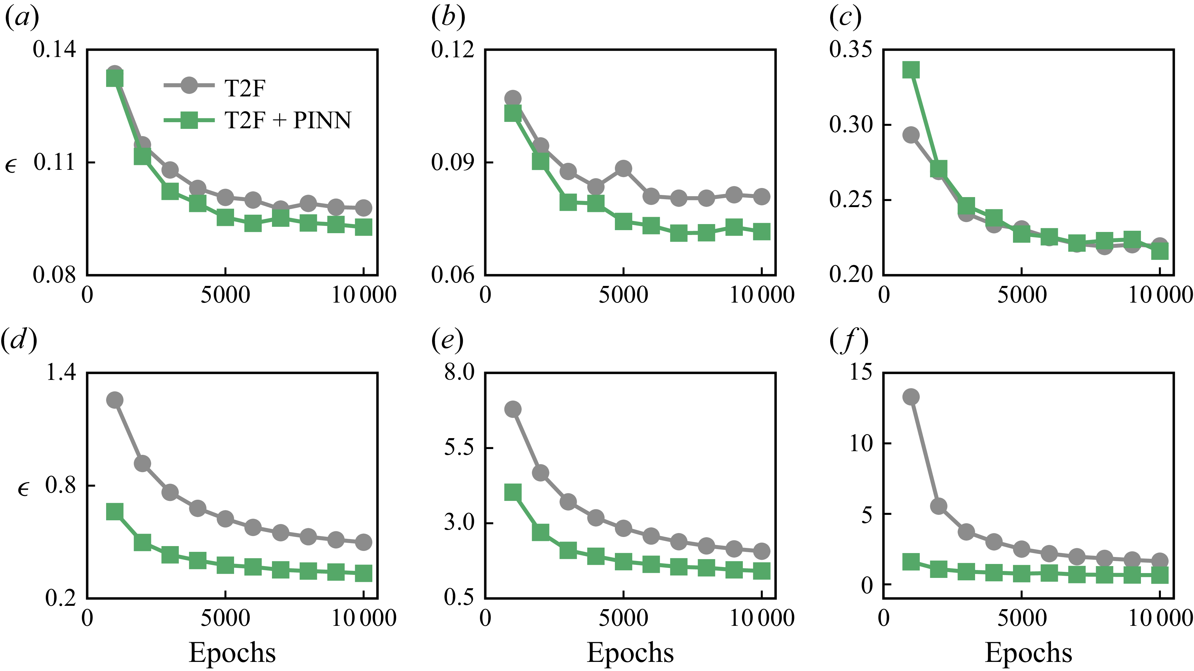
Figure 13 presents the evolution of the normalised
 $L_{2}$
error with respect to training epochs for both the T2F and T2F+PINN models, evaluated over all
 $n_{\textit{test}} = 1000$
samples in the test set. We consider both the primitive variables
 $u_x^{\ast }$
,
 $u_y^{\ast }$
and
 $T^{\ast }$
(see figure 13
a–c), as well as the gradient-related quantities including the vorticity
 $\omega _z^{\ast }$
, the horizontal temperature gradient
 $\partial _{x^{\ast }}T^{\ast }$
and the
 $Q$
value
 $Q^{\ast }$
(see figure 13
d–f). For the primitive variables, both models exhibit a decreasing trend in reconstruction error as training progresses. The T2F model reaches a final normalised
 $L_{2}$
error of approximately 0.09 for
 $u_x^{\ast }$
, 0.08 for
 $u_y^{\ast }$
and 0.21 for
 $T^{\ast }$
at 10 000 epochs. The corresponding values for the T2F+PINN model are 0.09, 0.07 and 0.21, respectively. For the gradient-related quantities, the T2F+PINN model consistently outperforms the T2F model. At 10 000 training epochs, the T2F+PINN model achieves relative reductions in normalised
 $L_{2}$
error of 33.3 % for
 $\omega _z^{\ast }$
, 31.6 % for
 $\partial _{x^{\ast }}T^{\ast }$
and a substantial 60.1 % for
 $Q^{\ast }$
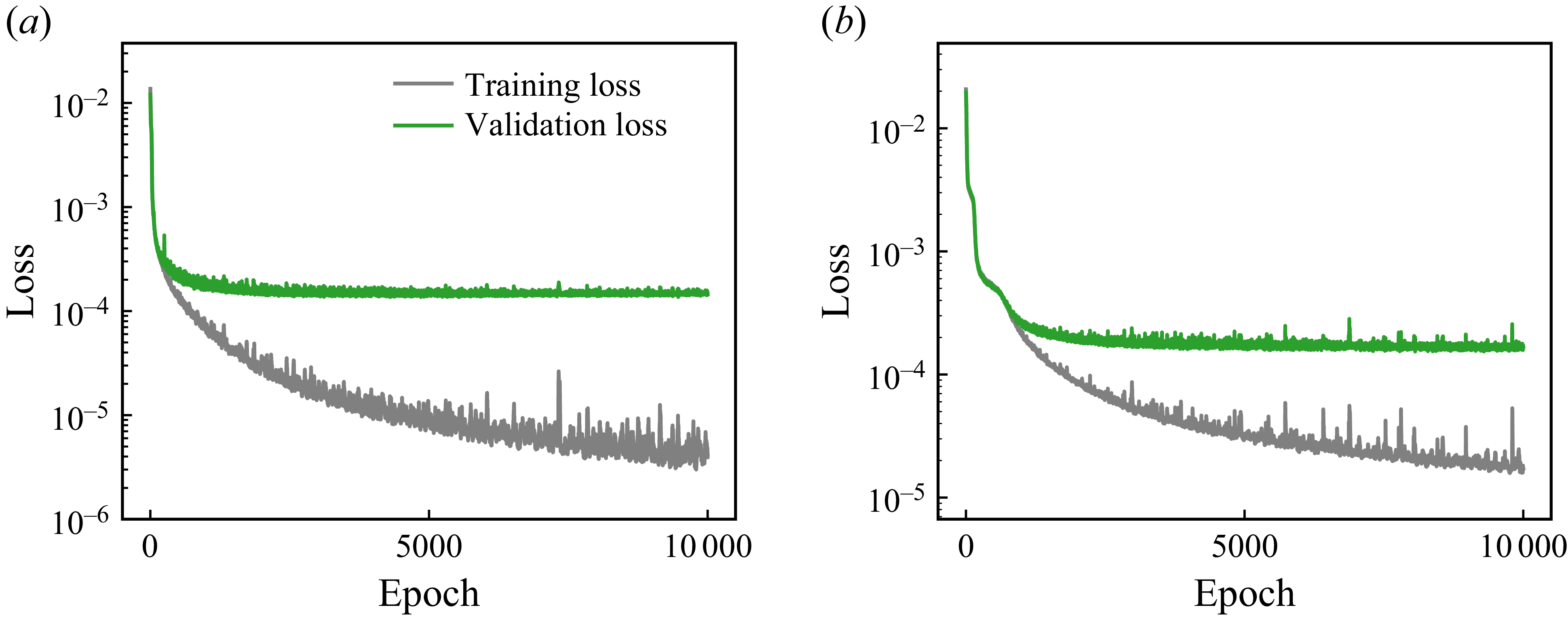
. These quantities involve spatial derivatives and are therefore more sensitive to local field smoothness and physical consistency, which are better preserved by the physics-informed constraints embedded in the T2F+PINN model. These results show that in the RB convection system, the T2F+PINN model excels in reconstructing gradient-based quantities, while the purely data-driven T2F model shows minor advantages in reconstructing primitive variables. To demonstrate that the model has reached convergence, we also provide the corresponding training and validation loss curves in Appendix B. Those conclusions obtained for the
 $\varGamma = 2$
RB convection system are expected to generalise to larger
 $\varGamma$
systems; where the number of convection rolls increase with
 $\varGamma$
(Wang et al. Reference Wang, Verzicco, Lohse and Shishkina2020b
), and the agents migrate a longer distance in the horizontal direction to mimic the behaviour of long-distance-migrating birds or patrolling UAVs (Xu et al. Reference Xu, Wu and Xi2023).
Evolution of the normalised
 $L_{2}$
errors over training epochs for the T2F and T2F+PINN models in RB convection. (a–c) The primitive variables
 $u_x^{\ast }$
,
 $u_y^{\ast }$
and
 $T^{\ast }$
. (d–f) The gradient-based quantities
 $\omega _z^{\ast }$
,
 $\partial T^{\ast } / \partial x^{\ast }$
and
 $Q^{\ast }$
. Results are compared between the T2F and T2F+PINN models.

Normalised
 $L_{2}$
errors
 $\epsilon$
of the reconstructed primitive variables (a)
 $u_x^{\ast }$
, (b)
 $u_y^{\ast }$
and (c)
 $T^{\ast }$
, and gradient-based quantities (d)
 $\omega _z^{\ast }$
, (e)
 $\partial T^{\ast } / \partial x^{\ast }$
and ( f)
 $Q^{\ast }$
as functions of input noise levels
 $\eta$
, for the T2F and T2F+PINN models in RB convection.

We also test the influence of input noise on the T2F and T2F+PINN models by computing the average reconstruction error over the entire test set, consisting of
 $n_{\textit{test}} = 1000$
samples in RB convection. Noise is added to the input variable in the test set, which consists of the velocity components
 $(u_x, u_y)$
and temperature
 $T$
, following the procedure described in § 3. Figure 14 shows the variation of the normalised
 $L_{2}$
error
 $\epsilon$
with respect to the noise amplitude
 $\eta$
for primitive variables
 $u_x^{\ast }$
,
 $u_y^{\ast }$
,
 $T^{\ast }$
, and for the gradient-based quantities
 $\omega _z^{\ast }$
,
 $\partial T^{\ast } / \partial x^{\ast }$
,
 $Q^{\ast }$
. As shown in figure 14(a–c), both models exhibit a gradual increase in error for the primitive variables as the noise level rises, and their performance remains broadly comparable across the full range of
 $\eta$
. In contrast, for the gradient-based quantities (see figure 14
d–f), the T2F+PINN model consistently outperforms the T2F model, with its error increasing at a slower rate. These results are consistent with the findings in the cylinder wake case (see figure 9), where the T2F+PINN model demonstrates enhanced robustness in reconstructing gradient-based quantities under noisy input conditions.
Next, we investigate the robustness of the T2F and T2F+PINN models under varying patch size
 $l_p$
for the RB convection case. The results for the T2F and T2F+PINN models for
 $l_p = 1$
,
 $2$
,
 $4$
and
 $8$
grid points are shown in table 2. Similar to the result in the cylinder wake, the reconstruction errors for both models remain relatively stable across different patch sizes. The T2F model exhibits a maximum variation of about 9 % in the reconstruction errors of
 $u_x^{\ast }$
,
 $u_y^{\ast }$
and
 $T^{\ast }$
, and the T2F+PINN model shows a slightly larger maximum variation of about 18 % in the reconstruction errors. Overall, the T2F and T2F+PINN models demonstrate robust performance across a range of patch sizes in the RB convection case as well.
Normalised
 $L_2$
errors of the reconstructed velocity components and temperature fields in RB convection for different patch sizes
 $l_p$
. The results are averaged over
 $n_{\textit{test}}=1000$
test samples.
Finally, we examine how sensitive the reconstructions are to changes in the control parameters of the RB system. Additional RB simulations are performed with Rayleigh numbers spanning
 $Ra=10^{7}$
–
 $10^{9}$
and aspect ratios ranging from
 $\varGamma =1$
to 8, while holding
 $\textit{Pr}=0.71$
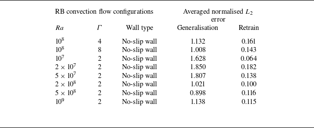
fixed. As shown in Appendix C, a model trained on a single reference case (here
 $Ra=10^{8},\,\varGamma =2$
with no-slip sidewalls) does not transfer reliably to flows at different
 $Ra$
,
 $\varGamma$
or wall conditions. Direct application to new configurations yields large normalised
 $L_{2}$
errors and often misses the correct large-scale structures. In contrast, retraining on the target configuration consistently restores accuracy, typically reducing errors by approximately an order of magnitude. These observations indicate that the present models mainly encode trajectory–flow correspondences specific to the training regime, so accurate reconstructions in practice require retraining (or at least fine-tuning) on flows with similar dynamical characteristics.
5. Conclusion
In this work, we proposed a deep-learning model, T2F, for reconstructing flow fields from sparse, localised trajectories of actively navigating Lagrangian agents. The model adopts an encoder–decoder architecture, where a ViT encoder captures both local and long-range temporal dependencies in agent motion, and a CNN decoder reconstructs the corresponding spatial flow structures. This design enables the extraction of rich spatiotemporal representations from limited Lagrangian input. To enhance physical fidelity, we further developed a physics-informed variant, the T2F+PINN model, by augmenting the data-driven loss with equation residuals derived from the governing physical laws. This integration of physics-based knowledge into the training process promotes reconstructions that are not only data-consistent but also dynamically coherent.
We first validated the model using a laminar cylinder wake flow as a proof-of-concept test. The T2F model demonstrated high accuracy in reconstructing the velocity field, while the T2F+PINN model significantly improved the reconstruction of vorticity. The T2F model outperformed the T2F+PINN model in estimating primitive variables due to its purely data-driven optimisation, whereas the T2F+PINN model achieved greater accuracy in reconstructing gradient-based quantities by incorporating physical constraints. Under varying levels of input noise, the T2F+PINN model exhibited enhanced robustness, showing markedly lower error growth in vorticity reconstructions even under strong input perturbations.
We then applied the model to turbulent RB convection, which is a paradigm system for convective flow in the atmosphere and oceans. Both the T2F and T2F+PINN models accurately reconstructed the primitive variables
 $u_x^*$
,
 $u_y^*$
and
 $T^{\ast }$
, but exhibited markedly different performance in gradient-related quantities. The T2F+PINN model consistently achieved superior reconstruction accuracy in vorticity, temperature gradients and the
 $Q$
value, outperforming T2F by up to 60.1 % in normalised
 $L_{2}$
error. These results highlight the capability of the T2F model to infer temperature and velocity structures in regions adjacent to sparse Lagrangian trajectories, while the T2F+PINN model offers a robust solution for applications requiring accurate inference of physically derived quantities.
Beyond demonstrating reconstruction accuracy, our results provide broader insights into Lagrangian sensing and data-driven flow reconstruction in turbulent environments. We open a promising avenue for real-time, physics-consistent inference of flow structures from sparse, localised observations. Owing to its data efficiency and robustness, the proposed model is particularly well suited for environmental perception tasks in scenarios where global field measurements are unavailable, such as soaring flight or underwater navigation. Looking ahead, our models can be extended to dynamic flow environments by incorporating online-learning strategies that adapt a pre-trained model using only physics-based loss functions, thereby eliminating the need for additional labelled data. It is also worth mentioning that the recently developed novel knowledge-integrated additive approach by Zhang et al. (Reference Zhang, Zhou, Yang and He2025) sheds light on the integration of physics and machine learning, and may enhance reconstruction by additively embedding domain-specific physical constraints directly into our T2F model.
Supplementary movies
Supplementary movies are available at https://doi.org/10.1017/jfm.2025.11033.
Acknowledgement
The authors acknowledge the Beijing Beilong Super Cloud Computing Co. Ltd for providing HPC resources that have contributed to the research results reported within this paper (http://www.blsc.cn/).
Funding
This work was supported by the National Natural Science Foundation of China (NSFC) through grant nos. 12272311, 12388101, 12125204; the Young Elite Scientists Sponsorship Program by CAST (2023QNRC001); and the 111 project of China (project no. B17037).
Declaration of interests
The authors report no conflict of interest.
Appendix A. The T2F model architecture
Here, we provide a detailed description of the T2F model architecture, which is based on a ViT encoder and a CNN decoder.
-
(i) Tokenisation, patch embedding and position embedding.
The ViT processes the input tensor as follows. For each instant
 $t = 1, \ldots , l_t$
, the ViT extracts a local spatial patch of size
 $l_p \times l_p$
with
 $C$
physical variables. Flattening this patch yields a vector of length
 $d_p = l_p^{2}C$
, referred to as a token. Collecting tokens across all time steps
 $l_t$
produces the input tensor
 $x_{\textit{token}}\in \mathbb{R}^{l_t \times d_p}$
. This input tensor is then linearly projected into a higher-dimensional space through a linear layer, a process referred to as patch embedding. The transformation is expressed as
 \begin{equation} x_{\textit{embed}} = x_{\textit{token}} W_e + b_e,\qquad W_e\in \mathbb{R}^{d_p \times d_e},\;\; b_e\in \mathbb{R}^{d_e}, \end{equation}
where
 $d_e$
is the embedding dimension,
 $W_e$
is a learnable weight matrix and
 $b_e$
is a learnable bias vector (broadcast and added to each token). Finally, a sequence of
 $l_t$
learnable positional embeddings is added to incorporate temporal positional information, yielding
 \begin{equation} x_{\textit{pos}} = x_{\textit{embed}} + p_e,\qquad p_e\in \mathbb{R}^{l_t \times d_e}, \end{equation}
where
 $p_e$
is a learnable positional embedding matrix.
-
(ii) Vision transformer encoder.
The ViT contains
 $n_{\textit{trans}}$
subencoder layers. After patch and positional embedding, the first subencoder layer takes
 $x_{\textit{pos}}$
as input, and its output is subsequently passed to the next subencoder layer. Each subencoder layer employs multi-head self-attention (MSA) to extract spatiotemporal features from the input
 $x_{\textit{in}}$
.
The MSA layers compute the attention scores between all pairs of input tokens. The computation is performed across
 $h$
heads in parallel. For each head
 $h_i$
, the input tensor
 $x_{\textit{in}}$
is projected into three matrices:
 \begin{equation} Q_i = x_{\textit{in}} W_{Q_i}, \quad K_i = x_{\textit{in}} W_{K_i}, \quad V_i = x_{\textit{in}} W_{V_i} ,\end{equation}
where
 $W_{Q_i}$
,
 $W_{K_i}$
and
 $W_{V_i}$
are learnable weight matrices for the query, key and value matrices, respectively. The attention scores are then computed as
 \begin{equation} \text{Attention}(Q_i, K_i, V_i) = \text{softmax}\left (\frac {Q_iK_i^{T}}{\sqrt {d_k}}\right )V_i ,\end{equation}
where
 $d_k$
is the dimension of the key vectors. The outputs of all heads are concatenated and projected back to the original input dimension:
 \begin{equation} x_{\textit{attn}} = \text{concat}(Z_1, Z_2, \ldots , Z_h)W_O ,\end{equation}
where
 $Z_i = \text{Attention}(Q_i, K_i, V_i)$
and
 $W_O$
is a learnable weight matrix.
Each MSA layer is followed by a feed-forward network (FFN) with layer normalisation. The FFN applies a nonlinear transformation consisting of two linear layers with a ReLU activation function:
 \begin{equation} x_{\textit{FFN}} = \text{ReLU}(x_{\textit{attn}}W_{\textit{FFN1}} + b_{\textit{FFN1}})W_{\textit{FFN2}} + b_{\textit{FFN2}} ,\end{equation}
where
 $W_{\textit{FFN1}}$
and
 $W_{\textit{FFN2}}$
are learnable weight matrices, and
 $b_{\textit{FFN1}}$
and
 $b_{\textit{FFN2}}$
are learnable bias vectors. The final output of the layer is normalised as
 \begin{equation} x_{\textit{out}} = \text{LayerNorm}(x_{\textit{in}} + x_{\textit{FFN}}), \end{equation}
where
 $\text{LayerNorm}$
normalises each token’s feature vector across the embedding dimension by computing its mean and variance. The final output of the ViT encoder is a tensor,
 $x_{\textit{ViT}}\in \mathbb{R}^{l_t \times d_e}$
, which represents a latent embedding of the input sequence. This latent representation is a learned feature with no explicit physical meaning. For further details of the ViT, we refer the reader to Dosovitskiy et al. (Reference Dosovitskiy2021).
-
(iii) Convolutional neural network decoder.
The output
 $x_{\textit{ViT}}$
is linearly projected and reshaped to a three-dimensional tensor of shape
 $l_{w0} \times l_{w0} \times C_0$
, where
 $C_0$
is the number of channels. This reshaped tensor is then processed by
 $n_{\textit{CNN}}$
transposed convolutional layers, each followed by a ReLU activation function. These transposed convolutional layers upsample the feature maps to the desired output resolution. For an input
 $x \in \mathbb{R}^{H_{\textit{in}} \times W_{\textit{in}} \times C_{\textit{in}}}$
, the transposed convolution operation is defined as
 \begin{align} y_{c_{\textit{out}}}[i,j] = \!\sum _{c_{\textit{in}}=0}^{C_{\textit{in}}-1} \sum _{m=0}^{H_{\textit{in}}-1} \sum _{n=0}^{W_{\textit{in}}-1} x_{c_{\textit{in}}}[m,n] W_{\textit{CNN}}[c_{\textit{in}}, c_{\textit{out}},\, i - ms \!+\! p,\, j - ns + p]\! +\! b_{c_{\textit{out}}} ,\end{align}
where
 $y_{c_{\textit{out}}}[i,j]$
is the output feature map at channel
 $c_{\textit{out}}$
and location (
 $i,j$
). The kernel
 $W_{\textit{CNN}}$
has shape
 $C_{\textit{in}} \times C_{\textit{out}} \times K \times K$
, with
 $K$
the kernel size,
 $s$
the stride and
 $p$
the padding along height and width.
The final transposed convolutional layer is followed by a standard convolutional layer to produce the output tensor. For an input
 $x\in \mathbb{R}^{H_{\textit{in}} \times W_{\textit{in}} \times C_{\textit{in}}}$
, the convolution operation is given by
 \begin{align} y_{c_{\textit{out}}}[i,j] = \sum _{c_{\textit{in}}=0}^{C_{\textit{in}}-1} \sum _{m=0}^{K-1} \sum _{n=0}^{K-1} x_{c_{\textit{in}}}[\,\textit{is} - p + m,\; \textit{js} - p + n\,]\, W_{\textit{CNN}}[c_{\textit{out}}, c_{\textit{in}}, m, n] + b_{c_{\textit{out}}}, \end{align}
with notations consistent with those of the transposed convolution. Further details of these operations are provided in Li et al. (Reference Li, Liu, Yang, Peng and Zhou2021).
Hyperparameters used in the T2F and T2F+PINN models.

Architecture of the CNN decoder in the T2F model. The transposed convolutional layers progressively upsample the feature maps to the target resolution
 $l_w$
.

The final output is a tensor
 $x_{\textit{CNN}}$
of shape
 $l_{w} \times l_{w} \times C$
, where
 $l_{w}$
is the output resolution and
 $C$
is the number of channels (
 $C = 2$
for the cylinder wake and
 $C = 3$
for RB convection). The detailed parameters of each layer are shown in figure 15.
The hyperparameters of the T2F and T2F+PINN models are summarised in table 3, including the input trajectory length, patch size, number of transformer layers and attention heads, CNN layers, batch size, learning rate and number of training epochs. With these settings, the T2F model contains approximately
 $2.1\times 10^8$
trainable parameters (
 $\approx \! 811$
MB). The computational cost for training a single T2F model takes about 4 h on an NVIDIA P100 GPU (16 GB).
Appendix B. Convergence of the T2F and T2F+PINN models
Here we provide the temporal evolution of both the training and validation losses for the T2F and T2F+PINN models in the cylinder wake case (see figure 16). For completeness, the corresponding loss histories for RB convection have also been included (see figure 17). Both figures show that, for both models, the validation losses decrease and then plateau after approximately 2000 epochs, indicating that the optimisation reaches a stable minimum. This demonstrates that the training of the T2F and T2F+PINN models converges satisfactorily, and that the fluctuations observed in figure 6(a,b) reflect variations in test-set performance rather than instability of the training process.
Evolution of the training loss and validation loss for (a) T2F model and (b) T2F+PINN model in the cylinder wake case.

Evolution of the training loss and validation loss for (a) T2F model and (b) T2F+PINN model in the RB convection case.

Appendix C. Robustness of the T2F model across different RB convection
The control parameters in the RB convection system include the Rayleigh number
 $Ra$
, the Prandtl number
 $\textit{Pr}$
and the aspect ratio
 $\varGamma$
. To assess the robustness of the T2F model across different RB convection, we conducted additional simulations in which we either apply the same trained T2F model (see § 4, trained on
 $Ra = 10^{8}$
,
 $\textit{Pr} = 0.71$
,
 $\varGamma = 2$
, no-slip sidewalls) to different RB configurations (hereafter referred to as ‘generalisation’), or retrain the model on each new configuration (hereafter referred to as ‘retrain’). The reconstruction accuracy was assessed using the normalised
 $L_2$
error of the velocity components
 $u_x^*$
.
Averaged reconstruction
 $L_2$
error over 1000 test samples for generalisation and retraining in an RB cell with
 $Ra=10^{8}$
,
 $\varGamma =2$
and periodic boundary condition for sidewalls.

-
Case (i). Similar flow field with plumes rising in the middle.
Averaged reconstruction
 $L_2$
error over 1000 test samples for generalisation and retraining in an RB cell with
 $Ra=10^{8}$
and
 $\varGamma =1$
.

We replaced the no-slip sidewalls with periodic boundary conditions and selected a time period with central plume upwelling for testing. Figure 18 shows the corresponding trajectories and reconstruction results. As summarised in table 4, the generalised model failed to reproduce the correct flow structures, whereas the retrained model achieved accurate reconstructions.
-
Case (ii). Flow transition from double rolls to a single large roll.
(a) Trajectories of self-propelling agents and temperature contours in an RB cell with
 $\varGamma =2$
and periodic boundary condition on the sidewalls. (b) Ground-truth field of horizontal velocity
 $u_x^*$
for a typical sample. (c) Reconstruction from the retrained model. (d) Reconstruction from the generalised model. Listed values indicate the normalised
 $L_2$
error.

We set the aspect ratio
 $\varGamma =1$
, where the flow exhibits a single-roll state. Due to the reduced domain size, only shorter trajectories were available, making generalisation infeasible. As shown in figure 19 and table 5, reliable reconstruction was achieved after retraining.
-
Case (iii). Different aspect ratios and/or Rayleigh numbers.
(a) Trajectories of self-propelling agents and temperature contours in an RB cell with
 $\varGamma =1$
. (b) Ground-truth field of horizontal velocity
 $u_x^*$
for a typical sample. (c) Reconstruction from the retrained model. Listed values indicate the normalised
 $L_2$
error.

We tested cases with aspect ratio
 $\varGamma = 4{-}8$
and Rayleigh number
 $Ra$
ranging from
 $10^7$
to
 $10^9$
(see figures 20 and 21 and table 6). Across these conditions, generalisation errors remained large, while retrained models consistently reduced errors by an order of magnitude.
Averaged reconstruction
 $L_2$
errors over 1000 test samples for generalisation and retraining in RB cells with different aspect ratio
 $\varGamma$
and Rayleigh number
 $Ra$
.

(a) Trajectories of self-propelling agents and temperature contours in an RB cell with
 $Ra=10^{8}$
and
 $\varGamma =8$
. (b) Ground-truth field of horizontal velocity
 $u_x^*$
for a typical sample. (c) Reconstruction from the retrained model. (d) Reconstruction from the generalised model. Listed values indicate the normalised
 $L_2$
error.

(a) Trajectories of self-propelling agents and temperature contours in an RB cell with
 $Ra=10^{9}$
and
 $\varGamma =2$
. (b) Ground-truth field of horizontal velocity
 $u_x^*$
for a typical sample. (c) Reconstruction from the retrained model. (d) Reconstruction from the generalised model. Listed values indicate the normalised
 $L_2$
error.