1. Introduction
In its 2000 Millennium Declaration, the United Nations set eight Millennium Development Goals. One of these goals is to reduce by half the proportion of people without sustainable access to safe drinking water by 2015. At the beginning of 2000, one sixth of the world's population (1.1 billion individuals) was without access to improved water supply, and two fifths (2.4 billion people) lacked access to improved sanitation. The majority of these people live in Asia and Africa. In 2000, 62 per cent of the African population had access to safe drinking water and 60 per cent benefited from adequate sanitation, with higher coverage rates in urban than in rural areas (World Health Organization, 2000).
Providing within-residence tap water access to additional households requires costly investments in terms of network extension and construction of storage capacity. Correct prediction of change in overall residential demand once all currently non-connected households get access to tap water is thus important for water managers. Such prediction is often difficult, though, since households that currently do not have access to tap water are likely to have characteristics that differ from those of connected households. Hence, the assumption that newly connected households will behave in the same way as those currently connected is likely to be inaccurate, and may lead to wrong predictions. This particular question has never been investigated using appropriate econometric techniques, as far as we know.
There exists substantial evidence that households that do not have access to a piped water network are on the average poorer (and less educated) than households that enjoy a piped connection. Income and education levels are commonly found to be important explanatory factors behind the probability that a household has a piped connection, regardless of country. Depending on the country, other factors such as sex and marital status of the household head and availability and quality of other available water sources matter in explaining the decision of households to obtain a piped connection (see Nauges and Whittington, forthcoming, for a literature review). Household characteristics strongly influence the rate at which households are connected to piped water networks, as well as the level of household water use. Hence, the simple assumption that non-connected households that obtain a connection will behave in the same way as households that currently have a connection may often be wrong. This is, however, a common assumption made by policy makers or water managers when making predictions on water use under scenarios of improved piped water coverage. The purpose of this paper is to propose an appropriate econometric method to estimate the increase in consumption due to the connection while controlling for the fact that households in both groups (those currently connected and those not) have different characteristics. In particular, the assumption just stated, that water consumption of previously and newly connected households is of the same magnitude, will be investigated.
Our approach builds on regime-switching models as well as on the literature on average treatment effects and allows controlling for selection based on observed and unobserved covariates. This methodology was originally developed for studying the effectiveness of social programmes (for example the effectiveness of job training programmes) or ‘treatments’ in medicine (see for example Heckman et al., Reference Heckman, Tobias and Vytlacil2001b, Reference Heckman, Tobias and Vytlacil2003; Wooldridge, Reference Wooldridge2002: chapter 18). The main innovation of this paper is to show the usefulness of the same basic approach for assessing the impact of obtaining a connection on water use.
The model is applied to a cross section of 246 households from Dakar, Senegal, which includes both connected and non-connected households. The city of Dakar has been facing continuous and chronic water shortages since the 1960s. In 1996, local authorities engaged in a partnership with the private sector to improve the management of water services. Since then, investments have been made to increase production capacity and extend the drinking water distribution network through an increased number of private connections and public standposts (SONES, 2004).
The approach developed in this paper should be applicable in all countries in which the situation regarding access to water is similar to the one studied in Dakar, i.e., urban areas in medium and large cities of less developed countries with incomplete but expanding piped water coverage. In many large cities in China, India, Southeast Asia and Latin America a substantial share of the population is not yet connected to the piped water system and currently relies on other public sources (public wells or public taps for example). Many of these cities will soon be able to afford, and will soon actually provide, more extensive municipal piped water services, due to rising incomes (see Nauges and Whittington, forthcoming, for related discussions). The expected increase in water use following the extension of the piped network will thus be a crucial piece of information for water services managers in these cities. The magnitude of the change in water use following access of piped water services is, however, likely to be case specific, since the consumption of both connected and non-connected households depends on several factors including the quality of the current non-tap water service and on the quality of a new tap service (such as continuity and pressure for the piped water service and accessibility and quality of the water distributed at the public sources) and is thus very heterogeneous across cities.Footnote 1 As a consequence, the change in average water use after getting a tap connection, found in this study, should be considered representative of the city of Dakar only.
Our paper also adds to the existing literature on valuation of increased household water consumption in developing countries but differs in the questions addressed and the methodology used. Most existing studies are of two specific types: contingent valuation studies to derive willingness to pay for getting a house connection to a piped water network (for example Whittington et al., Reference Whittington, Briscoe, Mu and Barron1990a, Reference Whittington, Pattanayak, Jui-Chen and Bal Kumar2002) or hedonic price studies to infer the valuation of a piped connection through observations of house prices (North and Griffin, Reference North and Griffin1993; Daniere, Reference Daniere1994; Nauges et al., Reference Nauges, Strand and Walker2009; see Komives, Reference Komives2003, for a review). Other recent studies have derived estimates of the price elasticity of demand for (piped and non-piped) water (see Nauges and Whittington, forthcoming, for a literature review). Finally, this paper provides insights into household water use in one particular African country. Water studies building on African micro data are still rare (Whittington et al., Reference Whittington, Mu and Roche1990b; Whittington and Lauria, Reference Whittington and Lauria1991; and Larson et al., Reference Larson, Minten and Razafindralambo2006, are exceptions).
We discuss the background and data in section 2. In sections 3 and 4, we describe the modelling strategy and estimation procedure, respectively. The model specification is discussed in section 5, and estimation results are presented in section 6. Section 7 concludes the paper.
2. Background and data
In the early 1990s, the city of Dakar faced increasing problems with water supply interruptions in some neighbourhoods. Water shortage was the consequence of low levels of rainfall (starting in the 1960s) and inefficient production infrastructure. In order to finance rehabilitation and extension of the water network and to increase production capacity, this city engaged in a public–private partnership for the management of water production and supply. Among other things, water access has been improved for the poorest households through installation of additional public standposts and subsidy of water connections. Between 1996 and 2003, 74 per cent of new connections were provided free of charge. The subsidies associated with these free provisions (an average of 100,000 CFA (Communauté Financière d'Afrique) Francs per connection)Footnote 2 mainly benefited households living in the poorest districts of Dakar. However, some unconnected (poor) households that were eligible for subsidy did not apply for it, mainly because the bimonthly payment associated with current water service was considered to be too high.Footnote 3 Indeed, some households argued that it was easier for them to control water expenditure at the public standpost where water is charged by the bucket (see Whittington et al., forthcoming, for related discussions). The decision to obtain a water connection also depends on the quality of the service at the public standpost in general and the opening hours in particular (Briand et al., forthcoming). The policy of increased supply was accompanied by a demand-side management policy: an increasing block pricing scheme for water supplied at the tap was introduced in order to guarantee access (for connected households) to a minimum amount of water and to induce more efficient water use.
The population of surveyed households covers 11 districts or sub-districts in Dakar, Senegal. The survey was undertaken in 2005, and its main objective was to assess the effectiveness of the investment programme that had been launched in 1995 to improve population access to safe water. For that purpose, the districts that have been surveyed for the present study correspond to districts surveyed by the World Bank in 1997 to measure households’ willingness to pay for improved water access (see Lauria et al. Reference Lauria, Alfredo and Anthony1997). Information on the type of water access, quantity of water used and price of water and opinions about water quality were gathered for 302 households.Footnote 4 In addition, the dataset has been complemented by a large set of socio-economic variables (for details on background and survey, see Briand, Reference Briand2006). Importantly, these 11 districts are representative not of the entire city of Dakar but rather of poor city districts only.Footnote 5
The dataset for our empirical analysis comprises a subset of 246 households for which water consumption is observed. Information on water consumption is missing for the 56 unconnected households that rely on sources other than a public standpost (including water vendors and water bought from neighbours). However, we are confident that confining ourselves to the subset of households for which information on water consumption is available will not lead to significant selection bias. Mean comparison tests have shown that socio-economic and house characteristics (including education level of the household's head, whether the respondent knows how to read and write, ownership status and ownership of various devices in the house) were statistically indistinguishable, on average, between households getting water from a public standpost and households relying on other non-tap sources such as water vendors, wells or neighbours.Footnote 6 From this observation we infer that the sub-sample of households relying on public standposts can be considered a representative sample of unconnected households.
Among these 246 households, 57 per cent (139 households) obtain water from their own private taps (we do not know whether or not the household benefited from the subsidy programme).Footnote 7 In some cases, connected households may complement tap water with water bought from the public standpost.Footnote 8 The rest of our sample (107 households) are not tap connected and can obtain their water from a variety of sources, among which a public standpost is the most important.
At the time of the survey, each connected household had to show its latest bimonthly water bill to the interviewer and the total amount of the bill, as well as the household's water consumption (in cubic metres) during the last two months, and these variables were reported in the questionnaire. Households getting water from the public standpost (whether connected or unconnected) had to report the number (and capacity) of water buckets bought every day on average, along with the prices paid. In our sample, average water consumption for connected households is 60 L per capita per day (which for some connected households comprises water from both the tap and the public standpost) or, equivalently, 17 m3 per connected household per month. Average water use for non-connected household is 25 L per capita per day (or equivalently 6 m3 per household per month).
The result that average household water consumption is lower for non-connected households than for households with tap connections is intuitively reasonable. A tap connection provides easy and convenient water access and allows for a variety of water uses which are practically infeasible without such access; moreover, members of households that are not tap connected need to walk to the standpost (and wait in some cases) to haul water.Footnote 9 All uses requiring hot water such as using washers or perhaps even taking showers are far less convenient without tap access. Non-tap households may also have characteristics (e.g., low income) correlated with low water consumption. Differences in quality of the service for water provided at the tap with respect to water provided through non-tap sources may also be a reason why households using tap water have a higher consumption on average. For the particular case of Dakar, the service at the tap does not seem to offer full satisfaction though, since 45 per cent of connected households complain about frequent interruptions in water delivery and 32 per cent about insufficient pressure, while more than 50 per cent are not satisfied with colour and taste of water.Footnote 10 Finally, the average water price is much lower for tap water than for water bought at the public standpost. Water at the tap is charged according to a (unique) progressive price schedule with three main blocks: 0–20 m3, 20–40 m3 and above 40 m3. These blocks refer to bimonthly household consumption. Units in the first, second and third blocks are charged 191.32, 629.88 and 788.67 CFA Francs, respectively.Footnote 11 In our sample, the average water price for connected households is 477 CFA Francs per cubic metre, while non-connected households pay 974 CFA Francs per cubic metre on average at the public standpost.Footnote 12
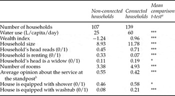
Households were also surveyed regarding their socio-economic characteristics, including household size, education, occupation and characteristics of the house including numbers of rooms, main material used for walls, roofs and floors, and water-consuming devices (shower, sink, washtub, toilets, etc.). The survey did not include any question on household income. This is likely not to be a major drawback, though, since household income in developing countries usually conveys only limited information about household standard of living (as it is frequently subject to misreporting and/or measurement error). For the purpose of our study, we built a wealth index using the principal components analysis (PCA) techniques, following the approach developed in Filmer and Pritchett (Reference Filmer and Pritchett2001). We retained 24 variables related to house characteristics (including material used for the roof, floor and walls) and equipment, which are supposed to be correlated with household wealth (see the appendix for greater detail on construction of the wealth index). Finally, each household was asked to record the distance from its home to the closest standpost, and households relying on public standposts were asked to give their opinion about the quality of the service provided. In the forthcoming empirical application, we will consider the average opinion about opening hours at the standpost in the district in which the household is situated; i.e., we take the average for all households in the district, of a dummy variable which is equal to 1 when the household thinks that the standpost has convenient opening hours, and 0 otherwise. Some average-sample characteristics are shown for connected and non-connected households in table 1.
Mean characteristics for connected and non-connected households

a *, ** and *** indicate significant differences between means in the two groups at the 10, 5 and 1 per cent level respectively.
b A higher value of this index indicates a better opinion about the service at the standpost.
We also report here the outcome of the Student test for mean comparison between the two groups. On average in our sample, connected households have houses with more rooms and a greater number of water-consuming equipments (such as showers and washtubs). Ninety-three per cent (57 per cent) of connected (non-connected) households are owner occupied. Also, connected households are on average better educated than non-connected households: 71 per cent of household heads of connected households are able to read, while only 45 per cent in the group of non-connected households can read. We also observed a higher proportion of widows as household heads, and larger families on average, in the group of connected households. Finally, connected households are in districts in which the average opinion about the service at the standposts is lower.
3. Modelling approach
The specification and estimation procedure builds on the literature on regime-switching models developed by Heckman (Reference Heckman1976; see also Heckman et al., Reference Heckman, Tobias and Vytlacil2001a, Reference Heckman, Tobias and Vytlacilb, and Wooldridge, Reference Wooldridge2002).Footnote 13
We denote by q 1i (resp. q 0i ) the (per-capita) water consumption of household i with a tap connection, d i = 1 (resp. without a tap connection, d i = 0). The quantity of interest here is the change in water use after household i obtains a tap connection: Δq i = q 1i −q 0i . But because household i cannot be in both states, we cannot observe both q 1i and q 0i . As a consequence of this missing data problem, we focus our attention on features of the distribution of Δq i = q 1i −q 0i . In particular, the quantities of interest estimated in the empirical application are the average treatment effect ATE ≡ E(q 1−q 0) and the average treatment effect on the treated TT ≡ E(q 1−q 0|d = 1). The ATE is designed to measure the expected effect of the ‘treatment’ (here, having a tap connection) on water consumption for a household drawn at random from the population. The TT is likewise designed to measure the mean effect on water consumption of having a tap connection, for those households that are actually tap connected.
If access to a tap connection were completely random across all households, then we would have ATE = TT = E[q|d = 1]−E[q|d = 0], where E[q|d = 1] (resp.E[q|d = 0]) is the sample average of per-capita water consumption for households with a tap connection (resp. without a tap connection). Put differently, if tap connections were randomized across households, then the expected change in water use after obtaining a tap connection could be consistently estimated by taking the differences between the two sample averages. But in most cases households at least have some influence on whether they obtain a tap connection. Their decision to obtain a tap connection is then probably related to the benefits of the connection: q 1−q 0 (this is the so-called self-selection into treatment).
A wide range of models have been proposed to derive measures of the ATE and TT while controlling for self-selection (see Wooldridge, Reference Wooldridge2002). In general, these models involve the use of observed covariates. However, when some important information is not observed in the data, conditioning on observed covariates is usually not sufficient to eliminate the effects of self-selection. In our particular case study, variables such as households’ health records, opportunity cost of time and time spent at home are not observed and are likely to be significant determinants of household water consumption. Our approach involves conditioning on observed covariates and controlling for self-selection. It requires the specification of water demand equations for both connected and non-connected households and the estimation of a selection equation to explain the decision of households to get a tap connection and relies on instruments to identify the effect of the tap connection on water use.
3.1. Water demand equations
We define two demand equations, one for connected households (k = 1) and one for non-connected households (k = 0):

The x-vector gathers all observable explanatory variables; c k is a constant; and u ki is the idiosyncratic error term with assumed mean zero. The ak -vector gathers unknown parameters of the demand function in the regime k = 0, 1; x corresponds to the sample average of x i . Water consumption for household i can equivalently be written:

This is a regime-switching equation which illustrates the fact that consumption of household i is only partially observed (in either one situation or the other).
3.2. Modelling the decision to obtain a tap connection
We need to specify an equation which describes the household's decision to obtain a tap connection. We assume that household i is tap connected if its utility with tap connection (V
1i
) is greater than its utility without tap connection (V
0i
).Footnote
14
Denoting by  the latent variable corresponding to the difference between V
1i
and V
0i
, we have

In this model, the error term e i is assumed to have mean zero, and the z-vector contains excluded variables from the demand equations (1). These variables will play the role of identifying restrictions for the effect of having a tap connection on households’ water use.
3.3. Full (and final) model
Equations (1)–(3) can be combined (see Wooldridge, Reference Wooldridge2002) and the full model is finally written:


We here allow for correlation between the unobserved components in equations (4) and (5). We assume that these error terms follow a trivariate normal distribution, as follows:Footnote 15

4. Estimation procedure
Estimation is done in two steps. In the first step, model (5) is estimated by maximum likelihood (ML) under the assumption that the error terms are normally distributed (probit approach). Under this assumption, the ML estimator is asymptotically consistent and efficient. The demand model (4) is estimated in the second step using ordinary least squares (OLS). We need to control for possible correlation between the error terms in the demand equation, u 0 and u 1, which capture unobservable determinants of water consumption, and the error term in the decision model (or selection equation), e i . If this correlation is different from zero, our parameter estimates will suffer from selection bias. To correct for potential selection bias, we incorporate two additional variables known as inverse Mills ratios and defined as follows:

where  correspond to the vector of estimated parameters in the probit model (5), and ϕ and φ are the standard normal probability density function and distribution function, respectively.
The two inverse Mills ratios enter the demand model as follows:

where ρ1σ1 and ρ0σ0 have been defined in (6) and
![\begin{equation}
\varepsilon _i \,{\equiv}\, (u_{1i} - u_{0i})d_i + u_{0i} - [ {\rho _1 \sigma _1 \lambda _1 ({\bf \hat b'z}_i)d_i - \rho _0 \sigma _0 \lambda _0 ({\bf \hat b'z}_i)(1 - d_i)} ].\]%\end{equation}](https://static.cambridge.org/binary/version/id/urn:cambridge.org:id:binary:20160920233619651-0344:S1355770X09990076:S1355770X09990076_eqnU1.gif?pub-status=live)
An attractive feature of this approach is that ATE and TT measures can be easily derived from parameter estimates in model (8). We have:

5. Model specification
Per-capita per-day water consumption is chosen as the dependent variable in the demand model (variable qi in model (8)). The x-vector applied in our final estimations includes the following variables: the household's wealth index, household size (number of household members) and an indicator variable which takes the value of 1 if the household head is a widow and 0 otherwise. The existing literature (see Nauges and Whittington, forthcoming) indicates that wealth has a positive effect on consumption, regardless of country. We thus expect the coefficient associated with the wealth index to exhibit a positive sign. The expected impact of household size on water consumption per capita is negative, due to economies of scale at the household level (see Nauges and Whittington, forthcoming). Indeed, the overall water consumption of a household increases less than proportional to the number of household members because a significant share of daily water use is independent of household size (e.g., washing up and cleaning of the floor). The status of the household head, in particular whether or not the household head is a widow, has been less frequently considered in the empirical literature. Briand et al. (forthcoming), using data from the same survey, have found that the widow status increases the probability of being connected to the piped water network. They explain this result by a higher opportunity cost of time for widows compared to married women (since they have to take care of the whole family and are responsible for all household affairs) and by women being more conscious about the risk of water-borne diseases. The latter effect is likely to dominate, so we would expect households with a widow at their head to have a higher water consumption, all other things equal.
As instruments (z-vector), we use an indicator variable which takes the value 1 if the house is rented and 0 otherwise, the distance between the house and the closest standpost, the average opinion about the standpost service in the district in which the household is and an indicator variable which takes the value 1 if the household has characteristics that make it eligible for a subsidized connection. We do not observe whether or not the household benefited from a subsidized connection, but since we know the eligibility criteria (see footnote 3), we are able to control for part of this unobservable characteristic. We define as ‘eligible’ a household that owns a house and is in the 40 per cent ‘poor category’, where the poor category is defined from the wealth index. The distance to the standpost, as well as the average opinion about the service provided at the standpost, should be suitable instruments, since they are likely to drive households’ decision to obtain a private connection, but should have no impact on the quantity of water used. The renter/owner status is chosen as an additional instrument, since, on the one hand, property titles are often required in order to get a tap connection. This variable should, on the other hand, have no influence on per-capita water use by the household.
As discussed earlier, the lack of cross-sectional variation in the pricing scheme in the group of connected households rules out the possibility that the price elasticity may be estimated in this model.Footnote 16 As for the group of non-connected households, some studies have considered as a potential determinant of water use the cost of water collection (Nauges and Strand, Reference Nauges and Strand2007). Conceivably, one could convert collection time into collection costs using the average wage of unqualified workers (with correction terms if children are in charge of water collection instead of adults) as a proxy for the unitary cost of time (Whittington et al., Reference Whittington, Mu and Roche1990b). This turned out to be difficult here for several reasons: First, collection time was not reported in the data, since households had only been questioned about the distance to walk to the public standpost. We are thus not able to control for waiting time at the source. Second, for most of the households in our sample, more than one household member is in charge of collecting the water. Since we do not know how collection time is shared between family members, it is difficult to compute the corresponding opportunity cost of time. Finally, because collection costs would have been strictly positive for non-connected households and zero for most connected households (except for the few who combine water from both sources), it would have been difficult to identify the effect on water use of having a tap connection at the final stage. For these reasons, collection costs were not computed and thus not included as covariates in the demand model. The variable which indicates whether the household's head is or is not a widow and the wealth index are however both proxies for the opportunity cost of time. Households with higher wealth typically have higher salaries and thus higher opportunity costs of time. A household head who is a widow may have a higher opportunity cost of time as well, since she is likely to be in charge of all in-house activities. Collection costs are an important variable which is missing from the list of observed covariates and will most likely be part of the error term in the demand equation.
6. Discussion of estimation results
6.1. First-stage model: estimation of the probit model to explain households’ decision to get a tap connection
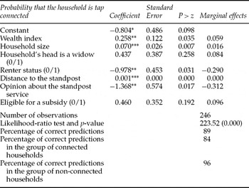
Estimation results are shown in table 2. We report estimated coefficients along with marginal effects. For each dichotomous variable, the marginal effect measures the change in the probability of having a connection following a change from 0 to 1 in the dichotomous variable (see Greene, Reference Greene2003: chapter 21). The latter is easier to interpret, since it provides a direct measure of the impact of each variable on the probability of having a tap connection. The model performs reasonably well, since 89 per cent of our predictions are correct, overall. The model gives very good predictions for both groups of households: 84 per cent for the group of connected households and 96 per cent for the group of non-connected households. Five out of the seven covariates are found to be significant and to have expected signs. A positive change in a household's wealth (as measured by the wealth index) increases the probability that the household has a tap connection (see Larson et al., Reference Larson, Minten and Razafindralambo2006, for similar findings using data from Madagascar). The rental status is also found to have a significant effect on the probability of being connected: the marginal effect on this probability is estimated at −0.29. A household with more members is more likely to have a connection. Finally, the greater the distance to the standpost and the lower the average opinion (in the district) about the service at the standpost, the higher the probability that households are connected to the piped network. The estimated parameters are used to compute the inverse Mills ratios, as shown in (7).
ML estimation results (probit model)

Note: *, ** and *** indicate significance at the 10, 5 and 1 per cent level respectively.
6.2. Second-stage model: estimation of the final demand model
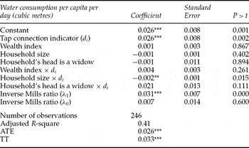
We apply OLS to the demand equation (8) in which inverse Mills ratios have been incorporated.Footnote 17 Estimation results are shown in table 3.
OLS estimation of the final model with selection bias correction

Note: *, ** and *** indicate significance at the 10, 5 and 1 per cent level respectively.
The adjusted R-squared is 0.41, and the Fisher test confirms overall significance of the model. The low number of significant parameters is still no surprise (and is quite common in such models) due to high collinearity between the variables in the x i − x vector and those in the x i − x )d i vector. We will thus comment only on the estimated ATE and TT measures, which are the main parameters of interest here. We find that the expected increase in water use after obtaining a tap connection for a person randomly drawn from the population (ATE) is 26 L per capita per day (this corresponds to the coefficient of the tap connection indicator times 1,000 to convert it into litres). This average effect is lower than the difference between the sample means of per-capita water use (between the group of connected households and the group of non-connected households) which is 35 L per capita per day (computed as 60 − 25). This latter result illustrates that the simple comparison of sample averages is likely to yield quite misleading predictions in terms of expected change in consumption after obtaining a tap connection.
The expected effect of obtaining a connection on the group of connected households (TT) is 33 L per capita per day. This is somewhat higher than the expected water consumption increase resulting from a connection, for the population as a whole (ATE). This difference, between the TT and ATE, which amounts to 33 − 26 = 7 L, represents a measure of the extent of self-selection. Significant self-selection effects indicate that households’ decision to obtain a tap connection depends on the difference in expected consumption with and without a tap connection. A positive self-selection effect indicates that households chose to be tap connected in order to enjoy a higher water consumption. Put differently, households that connected to tap did so because they on average had greater water needs than households that did not do so.
Some insights can be drawn from the decomposition of self-selection into self-selection based on observed covariates (1 L) and self-selection based on unobserved covariates (6 L).Footnote 18 Self-selection based on observed covariates means that some observable characteristics of currently connected households explain both their decision to obtain the connection and their higher per-capita consumption (by 1 L on average). From the set of estimates, it appears that household size is the most important characteristic here. Connected households have (on average) larger families than unconnected households (see table 1) and as a result greater total consumption of all household goods, including water. The latter was one reason for them to obtain the connection in the first place.
Self-selection based on unobserved covariates represents a 6-L difference between connected households and a randomly drawn household from the population. In other words, some unobservable characteristics explained both the choice of households to get a tap connection and their higher water consumption. Households with a tap connection are on average wealthier and more educated than households without a tap connection (see mean comparison tests in table 1). As a consequence, having immediate access to safe tap water tends to be valued highly by currently connected households, for which the opportunity cost of time is likely to be higher than for unconnected households (also since average salaries of the latter are lower). A further benefit of the connection, which is not directly observed in our data, could be in terms of improved water quality. Overall, water obtained through the tap is considered to be of better quality than water at the public standpost. Connected households are likely to value the expected benefits from a tap connection, in terms of improved water quality and reduced health risk, more highly.
7. Conclusion
In this paper, we have shown that regime-switching models, building on a framework established by Heckman (Reference Heckman1976), can prove useful in estimating the expected change in water use as a result of obtaining a tap connection for initially non-connected households. We applied this estimation procedure to a cross section of households in Dakar, Senegal. We have shown that obtaining a tap connection induces an expected increase in water use of 26 L per capita per day. If this figure is likely to be specific to the city of Dakar, the methodology described in this paper should be applicable in all urban areas in medium and large cities of less developed countries with incomplete but expanding piped water coverage. The accurate measurement of the expected increase in water use is necessary information for managers in the planning of future investments.
Using rigorous econometric techniques, we have found that the expected increase in water use is lower than the average difference in per-capita water use between the group of connected households and the group of non-connected households, which is 35 L per capita per day. This latter result illustrates that predicting the change in consumption after obtaining a tap connection from the simple comparison of sample averages can be quite misleading.
Our results also emphasize that characteristics of connected and unconnected households have to be taken into account when attempting to assess the impact on water demand when additional households are provided with tap water service. In particular, household size, household members’ opportunity cost of time and the expected health benefits following from a tap connection may all be important drivers, first, of the choice of getting a tap connection and, second, of water consumption. These variables may also explain, as was the case for our sample from the city of Dakar, that the average difference in water consumption between currently connected and unconnected households (+33 L per capita per day) is greater than the expected effect of one additional connected household (+26 L per capita per day). The latter result suggests that gains from obtaining a connection, for currently connected households in Dakar, to a large degree resulted from the increase in water use.Footnote 19 Further research is needed here to measure the impact of water price, collection costs (for non-tap water) and better quality on the decision of households to obtain a tap connection.
Appendix: Construction of a household wealth indicator using PCA
Description of the methodology
Suppose we have a set of N variables a*1j , . . ., a* ij , . . ., a* Nj assumed to be correlated with wealth for each household j. Each variable is normalized as follows: a 1j = (a 1j * − a 1*)/(s 1*), where a*1 is the mean of a*1j and s*1 is its standard deviation. Each of the standardized variables is then written as linear combinations of a set of underlying components (the As) for each household j (j = 1, . . ., J):

where νs are the (unknown) coefficients on each component for each variable. We follow the approach of Filmer and Pritchett (Reference Filmer and Pritchett2001) by considering only the first principal component (A 1j ) for the computation of the wealth index. The PCA allows us to determine the weight (f ij ) associated with each characteristic a ij (i = 1, . . ., N) so that the linear combination of the characteristics maximizes the variance of A 1j . The wealth index is then calculated for each household j as follows:

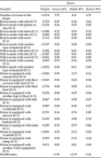
The list of the variables that we used to construct the wealth index is presented in table A1.
Variables and corresponding weights for the computation of the wealth index

Note: The first principal component explains 14.9% of the variation in the 24 variables.
Tests of reliability of the wealth index
Once the wealth index has been calculated, we sort individuals by this index and establish cut-off values for percentiles of the population. We then assign each household to a group on the basis of its index value. We refer to the bottom 40 per cent as ‘poor’, the next 40 per cent as ‘middle’ and the 20 per cent at the top as ‘rich’. We indicate in table A1 the weight assigned by the PCA to each variable, the sample average of each variable in each of the three groups of households and the average value of the wealth index in each of the three groups. The average wealth index is −1.95 in the group gathering the poorest households, −0.75 in the middle group and 5.41 in the group gathering the ‘richest’ households. The value of the index is as expected for most variables. For example, the proportion of roofs made with slab, the proportion of cement walls or the proportion of households equipped with shower increases with the level of the household's wealth. We also obtain consistent results when we calculate the proportion of households that can read and write in each of the three groups: 51 per cent of households belonging to the first group are able to read and write, 56 per cent in the middle group and 84 per cent among the group of richest households.