1. Introduction
Most developed and emerging countries have recently experienced the return of inflation and the multiplication of different exogenous shocks such as COVID-19, geopolitical tensions and wars, and climate change risk. These events have directly or indirectly impacted their entire economies and various sectors (Jawadi et al. Reference Jawadi, Rozin, Gnegne and Cheffou2024). These events have led to several successive crises and economic downturns, increasing financial vulnerability, public deficits, and debts, while exacerbating poverty and inequality, thereby impacting industries and consumer behaviour (Jawadi and Pondie, Reference Jawadi and Pondie2024). To explore the purchasing power, consumption behaviour, and economic well-being of households in a context characterised by high political and economic uncertainty, this study aims to track and analyse the dynamics of household consumption and expenditure as well as examine its evolution and drivers. This would help to quantify the impact of the recent crises and downturns on household consumption, model consumption dynamics, and identify suitable actions and economic policies to improve the householder’s well-being.
Based on this perspective, revisiting the relationship between household consumption and income is crucial, as it provides a relevant framework for understanding changes in consumer choices and individual financial behaviours and analysing the consumption–income lead-lag effects. Household consumption positively correlates with income, and that higher income leads to increased consumption and therefore high economic growth (Dufrénot and Mignon, Reference Dufrénot and Mignon2004). With an increase in income, householders are expected to afford better goods and services and to improve their quality of life (Jawadi and Sousa, Reference Jawadi and Sousa2014). Furthermore, an increase of housing income can also increase consumer spending (Piazzesi et al. Reference Piazzesi, Schneider and Tuzel2007; Aladangady, Reference Aladangady2017). However, a wealth or income shock might also imply a consumption adjustment. Consumption decisions always depend on the income and on a trade-off between investment and saving. Additionally, the consumption–income relationship often varies directly or indirectly with policies such as fiscal and monetary policies, which are continuously adjusted to account for uncertainties in the business cycle and economic shocks.
In the related economic theory literature, while most economists have always agreed with the existence of a significant relationship between consumption and income, they differ slightly with regard to the definition of income drivers and the channels explaining this relationship. First, Keynes (Reference Keynes1936) established a consumption function for which the household consumption depends basically on the disposable income that is defined as the income after tax. Keyne’s model provides a framework for short-term dynamics of consumption for which household consumption is basically driven by the disposable income. Accordingly, a tax cut would increase the disposable income and stimulate the consumption expenditures. Thus, as Keynes (Reference Keynes1936) stated in the psychological fundamental rule, the marginal propensity of consumption is always less than one, meaning that a 1% increase in disposable income yields less than a 1% increase in consumption.
Duesenberry (Reference Duesenberry1949) extended the Keynesian consumption theory by considering psychological factors and introducing habit formation as alternative key drivers for consumer choice. The life cycle hypothesis was next proposed by Modigliani and Brumberg (Reference Modigliani, Brumberg, Modigliani and Brumberg1954) to allow consumption to depend on lifetime income. This theory allows the consumption to vary differently with regard to the level of income or wealth earned by period or phase of life cycle.
Similarly, Friedman (Reference Friedman1957) proposed an alternative model to explain the dynamics of household consumption. Friedman’s theory relies on the permanent income hypothesis as a driver of household consumption, criticising the Keynesian hypothesis of disposable income. In particular, Friedman (Reference Friedman1957) identified two types of consumption and income: transitory and permanent components. Unlike Keynes (Reference Keynes1936), Friedman (Reference Friedman1957) showed that household consumption depends more on the permanent income rather than on the disposable income. Subsequent extensions of consumption models were also proposed (see Jawadi and Leoni, Reference Jawadi and Léoni2012, for more details).
Overall, these different consumption theories provided distinct economic frameworks to explain consumer behaviour and choice. Furthermore, they have yielded different empirical macro-econometric specifications and tests for the consumption function (Jawadi, Reference Jawadi2008). Additionally, the critique of Lucas (Reference Lucas and Lucas1976) and the related works of Hall (Reference Hall1978) and Deaton (Reference Deaton1985) significantly extended this consumption framework while considering the relevance of expectations and uncertainty to explain and model household consumption and expenditure. In addition, the stability/instability of consumption dynamics has opposed several economists. Milton Friedman argued that household consumption is unstable in the short-term but stable in the long-term. However, Deaton (Reference Deaton1992) introduced a theory known as the Paradox of Deaton showing that a change in non-expected income would not systematically lead to a significant change in household consumption. Thus, unlike Milton Friedman, Deaton (Reference Deaton1992) concluded that household consumption remains stable even in the short-term.
Empirically, the investigation between the consumption–income relationship has been the focus of various studies. Early studies specified this relationship in a linear framework using different econometric tests (Flavin, Reference Flavin1981; Johnson, Reference Johnson1986; Blanchard and Mankiw, Reference Blanchard and Mankiw1988; Constantinides, Reference Constantinides1990; Campbell and Mankiw, Reference Campbell and Mankiw1991; Cochrane, Reference Cochrane1994). Overall, these studies found that income constitutes a key driver of household consumption and that consumption is sensitive to changes in income and wealth. Furthermore, these previous studies often pointed to further evidence of stability in the relationship between consumption and income.
Within the attribution of Nobel Prize in Economics to Angus Deaton in 2015, in particular for his original work that proposes an econometric measure of individual behaviour in the domain of consumption, poverty, and well-being; several empirical works have focused and reconsidered the modelling of consumer behaviour and consumption dynamics using recent developments of macro-econometrics modelling. Accordingly, the (un)stability of the relationship between household consumption and its drivers was at the centre of debate of these studies (Ozak, Reference Ozak2014; Luo and Young, Reference Luo and Young2016). To model this further instability and asymmetry in the consumption—income linkage, several studies have relied on nonlinear models that allow different specifications of this relationship according to the state of the economy (Öcal and Osborn, Reference Öcal and Osborn2000; Dufrénot and Mignon, Reference Dufrénot and Mignon2004; Jawadi, Reference Jawadi2008; Jawadi and Léoni, Reference Jawadi and Léoni2012; Jawadi and Sousa, Reference Jawadi and Sousa2014).
Alan et al. (Reference Alan, Browning and Ejrnæs2018) highlighted significant heterogeneity and nonlinearity in the reaction of consumption to income shocks. This result is consistent with early findings of Öcal and Osborn (Reference Öcal and Osborn2000), who analysed consumption behaviour in the UK by estimating a univariate smooth transition autoregressive (STAR) model. Öcal and Osborn (Reference Öcal and Osborn2000) confirmed the nonlinear behaviour of consumption by identifying two business cycle regimes and showing that the consumption dynamics vary with the regime under consideration. Similarly, Lardic and Mignon (Reference Lardic and Mignon2003) investigated the relationship between consumption and income in the US, Germany, France, the UK, and Canada. The authors found significant evidence of nonlinearity in the relationship, suggesting that consumption—income relationship is unstable and time-varying. Öcal and Osborn (Reference Öcal and Osborn2000) and Jawadi (Reference Jawadi2008) also estimated a univariate STAR model and showed some evidence of nonlinearity and threshold effects in the consumption–income relationship for the US and France. This nonlinearity was justified by the presence of structural breaks caused by further jumps in habit formation. Jawadi and Sousa (Reference Jawadi and Sousa2014) showed a significant nonlinear and asymmetrical relationship between household consumption and the wealth that varies with the quantile under consideration. By considering a neoclassical growth model with habit formation, Jawadi and Leoni (Reference Jawadi and Léoni2012) also confirmed the nonlinear consumption behaviour and found that the consumption—income relationship exhibits asymmetry and nonlinearity.
Mian et al. (Reference Mian, Sufi and Khoshkhou2021) demonstrated that household consumption can react to changes in sentiment regarding government economic policy. Mian et al. (Reference Mian, Rao and Sufi2013) found that the debt and the geographic distribution of wealth shocks play a key role in explaining the significant and unequal decline in consumption during 2006–2009 in the USA. As shown by Mian and Sufi (Reference Mian and Sufi2014), both the Great Recession and Great Depression in 2009 were preceded by large levels of household debt and followed a collapse in asset prices and consumption.
Overall, these different empirical studies identified income, financial wealth, and interest rate as among the main drivers of household consumption. However, their estimations of the elasticity of consumption toward these drivers are not unanimously conclusive and rather depend on the data/sample under consideration. Furthermore, it appears that consumption elasticities always vary with the market state or regime.
Our study aims to revise the consumption–income relationship and explores the dynamics of household consumption, contributing to the related literature in two ways. On the one hand, in addition to the typical economic drivers (income and wealth), we specify the dynamics of household consumption by testing its reactions to changes in consumer sentiment. This is particularly relevant as it tests whether behavioural factors can help to improve modelling and forecasting consumer choice and expenditure. On the other hand, unlike previous studies that estimated the consumption–income relationship using a linear framework or univariate nonlinear model, we propose a nonlinear multivariate econometric specification to reproduce the relationship between household consumption and its drivers.
Our nonlinear multivariate framework presents different advantages. First, it enables the estimation of household consumption dynamics under the assumption of nonlinearity, asymmetry, and switching regimes. Second, our specification allows for threshold effects in the consumption–income relationship, which are identified endogenously. Third, we estimate the lead-lag effects between household consumption and its drivers in a nonlinear system, providing more consistent estimators. Fourth, rather than imposing an abrupt transition between consumption regimes, our model facilitates a smooth transition between regimes, capturing extreme states and a continuum of intermediate regimes. Finally, the thresholds and the number of regimes are specified using nonlinearity tests. To the best of our knowledge, this is the first study that specifies a vector logistic smooth transition regression (VLSTR) model to model the dynamics of household consumption.
The remainder of this paper is organised as follows. Section 2 briefly presents the econometric methodology. Section 3 discusses the main empirical results. Section 4 concludes the paper.
2. Econometric methodology
We rely on the class of the VLSTR model, which offers several advantages. First, it allows us to analyse the relationship between the consumption and its drivers in a system and therefore to assess for further lead-lag effects. Second, the VLSTR modelling allows us to model the relationship between household consumption and its drivers in a nonlinear framework. It enables us to capture the linkages between household consumption and its drivers while allowing this relationship to vary per state and to exhibit asymmetry, nonlinearity, and threshold effects. This is particularly relevant as it allows the consumption elasticities to vary with the regime under consideration. Consistent with Tersävirta and Yang (Reference Teräsvirta and Yang2014), the VLSTR model provides sufficient flexibility to test linearity and identify regimes through using linearity tests for different variables. The transition between regimes is also carried out differently using different transition functions for each equation of the system. Third, from an econometric perspective, this nonlinear multivariate framework provides more consistent estimators than does a univariate nonlinear framework.
2.1 Vector logistic smooth transition autoregressvie (VLSTAR) model
The linear Vector Auto-Regressive model with
 $k$
lags (VAR(
 $k$
)) is defined as:
 \begin{eqnarray*} \mathbf{y}_{t} &=&\mathbf{A}_{1}^{{\prime }}\mathbf{y}_{t-1}+\mathbf{A}_{2}^{{\prime }}\mathbf{y}_{t-2}+\cdots +\mathbf{A}_{k}\mathbf{y}_{t-k}+\mathbf{\Phi }^{{\prime }}\mathbf{d}_{t}+\mathbf{\epsilon }_{t} \\ &=&\mathbf{F}^{{\prime }}\mathbf{x}_{t}+\mathbf{\epsilon }_{t} \end{eqnarray*}
where:
 $\mathbf{F=(\mathbf{A}_{1}^{{\prime }},\mathbf{A}_{2}^{{\prime }},\ldots ,\mathbf{A}_{k}^{{\prime }},\mathbf{\Phi }^{{\prime }})}^{\prime }$
and
 $\mathbf{x}_{t}\mathbf{=(y_{t-1}^{{\prime }},y_{t-2}^{{\prime }},\ldots ,y_{t-k}^{{\prime }},d_{t}^{{\prime }})}^{{\prime }}$
. Furthermore,
 $\mathbf{d}_{t}$
is a vector consisting of deterministic components such as intercepts, trends and seasonal dummies, and exogenous variables and
 $\mathbf{\mathbf{\Phi }}$
contains the coefficients of the elements of
 $\mathbf{d}_{t}$
. The error vector
 $\mathbf{\epsilon }_{t}$
is assumed to be i.i.d.
 $N(0,\Omega ),$
where
 $\Omega$
is positive definite. However, this framework remains linear and cannot reproduce further asymmetry and nonlinearity in the data. Furthermore, it imposes a non-time varying constraint on the AR coefficients. To reproduce further asymmetry, the above linear VAR model can be generalised, following Yang (Reference Yang2012), into the VLSTAR model. The VLSTAR model corresponds to:
 \begin{equation} \mathbf{y}_{t}=\left \{ \sum \limits _{i=1}^{m}\left ( \mathbf{G}_{t}^{i-1}-\mathbf{G}_{t}^{i}\right ) \mathbf{F}_{i}^{{\prime }}\right \} \mathbf{x}_{t}+\mathbf{\epsilon }_{t} \end{equation}
where:
 $\mathbf{F=(\mathbf{A}_{i1}^{{\prime }},\mathbf{A}_{i2}^{{\prime }},\ldots ,\mathbf{A}_{ik}^{{\prime }},\mathbf{\Phi }_{i}^{{\prime }})}^{\prime }$
and
 $\mathbf{G}_{t}^{i}$
is a diagonal matrix of transition functions:
 \begin{equation} \mathbf{G}_{t}^{i}=diag\left \{ g\left ( s_{1it}|\gamma _{i1},c_{i1}\right ) ,\ldots ,g\left ( s_{pit}|\gamma _{ip},c_{ip}\right ) \right \} \end{equation}
for
 $i=1,\ldots ,m-1$
and
 $\mathbf{G}_{t}^{0}=I_{p},\mathbf{G}_{t}^{m}=0$
. The diagonal element of
 $\mathbf{G}_{t}^{i}$
in (2) are logistic functions of their transition variables
 \begin{equation} g\left ( s_{ijt}|\gamma _{ij},c_{ij}\right ) =\left ( 1+\exp \left \{ -\gamma _{ij}\left ( s_{ijt}-c_{ij}\right ) \right \} \right ) ^{-1},\gamma _{ij}\gt 0 \end{equation}
for
 $i=1,\ldots ,m-1$
and
 $j=1,\ldots ,p.$
The function (3) is a continuous (for
 $\gamma _{ij}\lt 1$
), monotonically increasing sigmoid function of its argument
 $s_{ijt}$
and bounded between zero and one. It is assumed that the transition variable
 $s_{ijt}$
is a weakly stationary random variable. Furthermore,
 $\gamma _{ij}$
is the slope parameter, or the smoothness parameter, determining the shape of the function, or the smoothness of the transition, and therefore measuring the transition speed between regimes. The parameter
 $c_{ij}$
is a location parameter determining the midpoint of the transition or the threshold.
The VLSTAR model can be reparameterised as follows:
 \begin{equation} \mathbf{y}_{t}=(\mathbf{B}_{1}^{{\prime }}+\mathbf{G}_{t}^{^{1}}\mathbf{B}_{2}^{{\prime }}+\cdots +\mathbf{G}_{t}^{^{m-1}}\mathbf{B}_{m}^{{\prime }})\mathbf{x}_{t}+\mathbf{\epsilon }_{t}=\mathbf{\Psi }_{t}^{{\prime }}\mathbf{B^{\prime }x}_{t}+\mathbf{\epsilon }_{t} \end{equation}
where
 $\mathbf{\Psi }_{t}=(\mathbf{I}_{p},\mathbf{G}_{t}^{^{1}},\ldots ,\mathbf{G_{t}^{^{m-1}}})^{{\prime }}$
is a
 $mp\times p$
full rank matrix. Furthermore,
 $\mathbf{B}=(\mathbf{B}_{1},\mathbf{B}_{2},\ldots ,\mathbf{B}_{m})$
is a (
 $kp\times q)\times mp$
matrix, where
 $\mathbf{B}_{1}=\mathbf{F}_{1}$
, and
 $\mathbf{B}_{i}=\mathbf{F}_{i}-\mathbf{F}_{i-1},i=2,\ldots ,m.$
The representation in (4) is equivalent to the one in (1). We observe that the representation in (1) describes the transition through different extreme regimes
 $\mathbf{F}_{i},i=1,\ldots ,m$
, while the reparametrized form in (4) is considerably easier for specification, estimation and evaluation, and hence it will be employed hereafter.
The modelling strategy for VLSTAR models, similar to that for univariate STAR models, comprises of three stages: Specification, Estimation and Validation. This strategy can be considered as a multivariate generalisation of the one discussed in Teräsvirta (1994, 1998). Estimating a linear VAR model is the first stage in specifying the VLSTAR model. This involves selecting the lag length for the VAR model using different tests, information criteria and autocorrelation functions. Specification comprises of testing the linear VAR model against the VLSTAR and, if linearity is rejected, determining the structure of the VLSTAR model. This implies selecting the transition variable(s) and determining the lag structure of the model. By so doing, joint tests of nonlinearity are used. If none of these tests rejects linearity, one can retain the linear VAR model. However, if the null hypothesis of linearity is rejected for at least one transition variable, the one producing the smallest p-value is chosen as an optimal transition variable. Furthermore, each equation is tested separately using the selected transition variable to determine whether some equations are linear.
In small samples, particularly when
 $p$
, the dimension of
 $y_{t}$
, is high, the LM type tests (of nonlinearity) of the
 $\chi ^{2}$
-family are likely to experience the problem of positive size distortion: the empirical size of the test exceeds the corresponding asymptotic size. To address this problem, three different versions of the test statistic are used. Two of them are based on Bartlett and Bartlett-type corrections. The first one is Wilks’s statistic using Wilks’s
 $\Lambda$
-distribution and the second one is Rao’s (Reference Rao1951, Reference Rao1965) statistic. Finally, a Wild Bootstrap (WB) testing procedure is employed to achieve the accuracy of the
 $p$
-values. The improvement of the WB test statistic appears to be satisfactory, though the computation is rather time-consuming.
2.2 Linearity tests
Testing a linear vector autoregressive (VAR) model against a nonlinear vector logistic smooth transition autoregressive (VLSTAR) is complicated by the unidentified nuisance parameters under the null hypothesis. Consequently, the asymptotic null distribution of the classical likelihood ratio, the Lagrange multiplier and the Wald type tests remain unknown. The solution of Luukkonen et al. (Reference Luukkonen, Saïkkonen and Teräsvirta1988b) and Luukkonen et al. (Reference Luukkonen, Saikkonen and Teräsvirta1988a) to this problem is to replace the transition function by a suitable Taylor series approximation. Yang (Reference Yang2012) generalises this approach to the multivariate case with a single transition variable.
Consider the
 $p$
-dimensional 2-regime logistic VSTAR model in (4):
 \begin{equation} \mathbf{y}_{t}=\mathbf{B}_{1}^{{\prime }}\mathbf{x}_{t}+\mathbf{G}_{t}\mathbf{B}_{2}^{{\prime }}\mathbf{x}_{t}+\mathbf{\epsilon }_{t} \end{equation}
where the sequence
 $\left \{ \mathbf{\epsilon }_{t}\right \}$
is i.i.d.
 $N(0,\Omega ).$
We rewrite the
 $\mathbf{G}_{t}$
matrix as:
 \begin{equation*} \mathbf{G}_{t}=diag\left \{ a_{1}s_{t}+b_{1}+r_{1t},\ldots ,a_{p}s_{t}+b_{p}+r_{pt}\right \} =\mathbf{As}_{t}+\mathbf{B}+\mathbf{R}_{t} \end{equation*}
where:
 $\mathbf{A}=diag\left \{ a_{1},\ldots ,a_{p}\right \} ,$
 $\mathbf{B}=diag\left \{ b_{1},\ldots ,b_{p}\right \}$
and
 $\mathbf{R}_{t}=diag\left \{ r_{1t},\ldots ,r_{pt}\right \} .$
Now we have:
 \begin{eqnarray} \mathbf{y}_{t} &=&\mathbf{B}_{1}^{{\prime }}\mathbf{x}_{t}+(\mathbf{As}_{t}+\mathbf{B}+\mathbf{R}_{t})\mathbf{B}_{2}^{{\prime }}\mathbf{x}_{t}+\mathbf{\epsilon }_{t} \nonumber \\ &=&\mathbf{(\mathbf{B}_{1}^{{\prime }}+B\mathbf{B}_{2}^{{\prime }})x}_{t}+\mathbf{AB}_{2}^{{\prime }}\mathbf{x}_{t}s_{t}+\mathbf{R}_{t}\mathbf{B}_{2}^{{\prime }}\mathbf{x}_{t}+\mathbf{\epsilon }_{t} \nonumber \\ &=&\mathbf{\Theta }_{0}^{{\prime }}\mathbf{x}_{t}+\mathbf{\Theta }_{1}^{{\prime }}\mathbf{x}_{t}s_{t}+\mathbf{\epsilon }_{t}^{\ast } \end{eqnarray}
where:
 $\mathbf{\Theta }_{0}=\mathbf{\mathbf{B}_{1}+\mathbf{B}_{2}B,}$
 $\Theta _{1}=\mathbf{B}_{2}\mathbf{A,}$
and
 $\mathbf{\epsilon }_{t}^{\ast }=\mathbf{R}_{t}\mathbf{B}_{2}^{{\prime }}\mathbf{x}_{t}+\mathbf{\epsilon }_{t}.$
Following Yang (Reference Yang2012), let:
 \begin{equation*} \mathbf{Y=}\left [ \begin{array}{c} \mathbf{y}_{1}^{{\prime }} \\ \mathbf{y}_{2}^{{\prime }} \\ \mathbf{\vdots } \\ \mathbf{y}_{T}^{{\prime }}\end{array}\right ] ,\mathbf{X=}\left [ \begin{array}{c} \mathbf{x}_{1}^{{\prime }} \\ \mathbf{x}_{2}^{{\prime }} \\ \mathbf{\vdots } \\ \mathbf{x}_{T}^{{\prime }}\end{array}\right ] ,\mathbf{Z}_{1}\mathbf{=}\left [ \begin{array}{c} \mathbf{x}_{1}^{{\prime }}s_{1} \\ \mathbf{x}_{2}^{{\prime }}s_{2} \\ \mathbf{\vdots } \\ \mathbf{x}_{T}^{{\prime }}s_{T}\end{array}\right ] \end{equation*}
and
 $\widetilde {\mathbf{B}}_{1}$
and
 $\widetilde {\Omega }$
are estimates from the restricted model,
 $\mathbf{P}_{x}=\mathbf{X}\left ( \mathbf{X}^{{\prime }}\mathbf{X}\right ) ^{-1}\mathbf{X}^{{\prime }}$
is the projection matrix, the following theorem can be applied for linearity test.
Theorem 1.
Consider the model in (
5
) and its reparametrization (
6
). Under the null hypothesis that
 $H_{0}\colon \gamma _{j}=0,j=1,\ldots ,p$
in (
5
), or equivalently,
 $H_{0}\colon \Theta _{1}=0$
in (
6
), the LM test statistic has the form:
 \begin{equation} \mathbf{LM}_{1}=\mathbf{tr}\left \{ \widetilde {\Omega }^{-1}\left ( \mathbf{Y}-\mathbf{X}\widetilde {\mathbf{B}}_{1}\right ) ^{{\prime }}\mathbf{Z}_{1}\left [ \mathbf{Z}_{1}^{{\prime }}(\mathbf{I}_{T}-\mathbf{P}_{x}\mathbf{)Z}_{1}\right ] ^{-1}\mathbf{Z}_{1}^{{\prime }}\left ( \mathbf{Y-X}\widetilde {\mathbf{B}}_{1}\right ) \right \} \end{equation}
Under the null hypothesis, the test statistic has an asymptotic
 $\chi ^{2}$
distribution with
 $p(kp+q)$
degree of freedom.
Consider now the VLSTAR model in which every equation can have its own transition variable,
 $s_{jt},j=1,\ldots ,p,$
and does not exclude the possibility that some equations in the system are linear. Linearity testing will then be carried out equation by equation. As there may be more than one transition variable candidate for any equation, we test the linearity for each of them. The basic rule of the VLSTAR model specification is to select the transition variable that produces the strongest rejection of linearity measured by the
 $p$
-value of the tests. If some equations have more than one reasonable transition variables after testing linearity, combinations of them could be considered.
2.3 Estimation of the VLSTAR
Both the nonlinear least squares (NLS) estimation and the maximum likelihood (ML) estimation of the parameters can be considered in the VLSTAR model. In both the NLS estimation and ML estimation, a grid search algorithm is employed to find a suitable starting value for the numerical optimisation. Yang (Reference Yang2012) showed the consistency and asymptotic normality of both the NLS estimator and the ML estimator under certain assumptions and conditions.
2.4 Specification of the VLSTAR
Evaluation of the model is done by three multivariate misspecification tests. They are the test of no serial correlation in the error process, the test of no additive nonlinearity and the test of parameter constancy. They are either Lagrange multiplier or Lagrange multiplier type tests. All of them are the extensions of the three univariate misspecification tests developed in Eitrheim and Teräsvirta (1996). We summarise the test statistics below. For more details and proof, see Yang and Teräsvirta (2014).
2.4.1 Test of no serial correlation in the error process
Assume the p-dimensional m-regime nonlinear VLSTAR model with autocorrelated errors
 \begin{equation} \mathbf{y}_{t}=\left \{ \sum \limits _{i=1}^{m}\left ( \mathbf{G}_{t}^{i-1}-\mathbf{G}_{t}^{i}\right ) \mathbf{F}_{i}^{{\prime }}\right \} \mathbf{x}_{t}+\mathbf{u}_{t}=\mathbf{\Psi }_{t}^{{\prime }}\mathbf{B^{\prime }x}_{t}+\mathbf{u}_{t} \end{equation}
where:
 \begin{equation} \mathbf{u}_{t}=\sum \limits _{i=1}^{J}\mathbf{P}_{i}^{{\prime }}\mathbf{u}_{t-i}+\mathbf{\epsilon }_{t}=\mathbf{P}(L)\mathbf{u}_{t}+\mathbf{\epsilon }_{t} \end{equation}
and
 $\mathbf{P}_{i}$
is a
 $p\times p$
matrix,
 $\mathbf{P}(L)=\sum \nolimits _{i=1}^{J}\mathbf{P}_{i}^{{\prime }}L^{i},$
 $L$
is the lag operator,
 $J$
is the lag length. By setting
 \begin{equation*} P\mathbf{=}\left [ \begin{array}{c} \mathbf{P}_{1} \\[3pt] \mathbf{P}_{2} \\[3pt] \mathbf{\vdots } \\[3pt] \mathbf{P}_{J}\end{array}\right ] ,z_{t}\mathbf{=}\left [ \begin{array}{c} \mathbf{y}_{t-1}-\mathbf{\Psi }_{t-1}^{{\prime }}\mathbf{B^{\prime }x}_{t-1} \\[3pt] \mathbf{y}_{t-2}-\mathbf{\Psi }_{t-2}^{{\prime }}\mathbf{B^{\prime }x}_{t-2} \\ \mathbf{\vdots } \\[3pt] \mathbf{y}_{t-J}-\mathbf{\Psi }_{t-J}^{{\prime }}\mathbf{B^{\prime }x}_{t-J}\end{array}\right ] =\left [ \begin{array}{c} \mathbf{u}_{t-1} \\[3pt] \mathbf{u}_{t-2} \\[3pt] \mathbf{\vdots } \\ \mathbf{u}_{t-J}\end{array}\right ] , \end{equation*}
the following theorem can be used to conduct the test of no serial correlation:
Theorem 2.
Consider the model (
8
). To test the null hypothesis
 $\mathbf{P}_{1}=\mathbf{P}_{2}=\cdots =\mathbf{P}_{J}=0$
, we obtain the LM test statistic
 \begin{equation} \mathbf{LM}=\mathbf{tr}\left \{ \widetilde {\Omega }^{-1}\widetilde {\mathbf{U}}^{{\prime }}\widetilde {\mathbf{Z}}\left [ \widetilde {\mathbf{Z}}^{{\prime }}\mathbf{I}_{T-J}-\widetilde {\mathbf{K}}\left ( \widetilde {\mathbf{K}}^{{\prime }}\widetilde {\mathbf{K}}\right ) ^{-1}\widetilde {\mathbf{K}}^{{\prime }}\widetilde {\mathbf{Z}}\right ] ^{-1}\widetilde {\mathbf{Z}}^{{\prime }}\widetilde {\mathbf{U}}\right \} \end{equation}
where:
 \begin{equation*} \widetilde {\mathbf{K}}\mathbf{=}\left [ \begin{array}{c} \mathbf{vec}\left [ \partial \left ( \widetilde {\mathbf{\Psi }}_{J+1}^{{\prime }}\widetilde {\mathbf{B}}^{{\prime }}\mathbf{x}_{J+1}\right ) /\partial \left ( \boldsymbol{\theta }\right ) \right ] ^{{\prime }} \\[3pt] \mathbf{vec}\left [ \partial \left ( \widetilde {\mathbf{\Psi }}_{J+2}^{{\prime }}\widetilde {\mathbf{B}}^{{\prime }}\mathbf{x}_{J+2}\right ) /\partial \left ( \boldsymbol{\theta }\right ) \right ] ^{{\prime }} \\ \mathbf{\vdots } \\[3pt] \mathbf{vec}\left [ \partial \left ( \widetilde {\mathbf{\Psi }}_{T}^{{\prime }}\widetilde {\mathbf{B}}^{{\prime }}\mathbf{x}_{T}\right ) /\partial \left ( \boldsymbol{\theta }\right ) \right ] ^{{\prime }}\end{array}\right ] ,\widetilde {\mathbf{Z}}\mathbf{=}\left [ \begin{array}{c} \widetilde {\mathbf{z}}_{J+1}^{{\prime }} \\[3pt] \widetilde {\mathbf{z}}_{J+2}^{{\prime }} \\[3pt] \mathbf{\vdots } \\[3pt] \widetilde {\mathbf{z}}_{T}^{{\prime }}\end{array}\right ] ,\widetilde {\mathbf{U}}\mathbf{=}\left [ \begin{array}{c} \widetilde {\mathbf{u}}_{J+1}^{{\prime }} \\[3pt] \widetilde {\mathbf{u}}_{J+2}^{{\prime }} \\[3pt] \mathbf{\vdots } \\[3pt] \widetilde {\mathbf{u}}_{T}^{{\prime }}\end{array}\right ] , \end{equation*}
and
 $\widetilde {\mathbf{z}}_{t}$
,
 $\widetilde {\mathbf{u}}_{t}$
and
 $\widetilde {\Omega }$
are estimated under the null hypothesis. Assume that the estimates of the parameters in
 $\boldsymbol{\theta }$
are constant. Under the null hypothesis, the test statistic (10) has an asymmetric
 $\chi ^{2}$
distribution with
 $Jp^{2}$
degrees of freedom.
2.4.2 Test of additive nonlinearity
The null hypothesis is that after fitting a VLSTAR model, there is no more nonlinearity left unmodeled. Consider the additive VLSTAR model
 \begin{eqnarray} \mathbf{y}_{t} &=&(\mathbf{B}_{1}^{{\prime }}+\mathbf{G}_{t}^{^{1}}\mathbf{B}_{2}^{{\prime }}+\cdots +\mathbf{G}_{t}^{^{m-1}}\mathbf{B}_{m}^{{\prime }})\mathbf{x}_{t}+\mathbf{G}_{t}^{^{m}}\mathbf{B}_{m+1}^{{\prime }}\mathbf{x}_{t}+\mathbf{\epsilon }_{t} \end{eqnarray}
 \begin{eqnarray} &=&\mathbf{\Psi }_{t}^{{\prime }}\mathbf{B^{\prime }x}_{t}+\mathbf{G}_{t}^{^{m}}\mathbf{B}_{m+1}^{{\prime }}\mathbf{x}_{t}+\mathbf{\epsilon }_{t} \end{eqnarray}
We estimate the
 $m$
-regime VLSTAR model in which the additive nonlinear term
 $\mathbf{G}_{t}^{^{m}}\mathbf{B}_{m+1}^{{\prime }}\mathbf{x}_{t}$
has been omitted and we test
 $H_{0}\colon \gamma _{mj}=0,j=1,\ldots ,p,$
against the alternative
 $H_{1}\colon$
at least one
 $\ \gamma _{mj}\gt 0.$
Additionally, the Taylor approximation of the transition function is used to deal with the problem, and similar test statistic can be obtained as in the linearity test in (7) .
2.4.3 Test of parameter’s constancy
A central assumption of the linear VAR and the VLSTAR models is that the parameters of the model are constant over time. Since the estimation of parameters is based on this assumption, it should be tested, and this holds for both linear and nonlinear models. Consider the following VLSAR model:
 \begin{equation} \mathbf{y}_{t}=\mathbf{\Psi }_{t}^{{\prime }}\mathbf{B}\left ( \tau \right ) \mathbf{^{\prime }x}_{t}+\mathbf{\epsilon }_{t} \end{equation}
where
 $\mathbf{B}\left ( \tau \right ) =\mathbf{B}_{a}+\mathbf{B}_{b}\lambda \left ( \tau |\gamma ,c\right )$
is a function of rescaled (normalised) time
 $\tau =t/T$
and
 \begin{equation*} \lambda \left ( \tau |\gamma ,c\right ) =\left ( 1+\exp \left ( -\gamma \left ( \tau -c\right ) \right ) \right ) ^{-1}-1/2 \end{equation*}
The null hypothesis of parameter constancy is
 $H_{0}\colon \lambda \left ( \tau |\gamma ,c\right ) =0.$
Using Taylor expansion, the model (13) is approximated and reparameterised as follows:
 \begin{equation} \mathbf{y}_{t}=\mathbf{\Psi }_{t}^{{\prime }}\mathbf{B_{a}^{\prime }x}_{t}+\mathbf{\Psi }_{t}^{{\prime }}\mathbf{B_{b}^{\prime }x}_{t}\tau +\mathbf{\epsilon }_{t}^{\ast } \end{equation}
where:
 $\mathbf{\epsilon }_{t}^{\ast }$
also contains the remainder
 $r_{t}$
from the Taylor expansion and
 $\mathbf{\epsilon }_{t}^{\ast }=\mathbf{\epsilon }_{t}$
under
 $H_{0}.$
The new null hypothesis is
 \begin{equation} H_{0}\colon \mathbf{B}_{b}=0 \end{equation}
Let
 $\widetilde {\mathbf{\Psi }},\widetilde {\mathbf{B}}_{a},$
and
 $\widetilde {\Omega }$
be estimated under the null. Denote
 $\widetilde {\mathbf{\epsilon }}_{t}=\mathbf{y}_{t}-\widetilde {\mathbf{\Psi }}_{t}^{{\prime }}\widetilde {\mathbf{B}}\mathbf{_{a}^{\prime }x}_{t},$
and
 $\widetilde {\mathbf{E}}=\left ( \widetilde {\mathbf{\epsilon }}_{1},\widetilde {\mathbf{\epsilon }}_{2},\ldots ,\widetilde {\mathbf{\epsilon }}_{T}\right ) ^{{\prime }}.$
Let
 \begin{equation*} \widetilde {\mathbf{Z}}\mathbf{=}\left [ \begin{array}{c} \mathbf{vec}\left ( \widetilde {\mathbf{\Psi }}_{1}\otimes \mathbf{x}_{1}\tau _{1}\right ) ^{{\prime }} \\[3pt] \mathbf{vec}\left ( \widetilde {\mathbf{\Psi }}_{2}\otimes \mathbf{x}_{2}\tau _{2}\right ) ^{{\prime }} \\[3pt] \mathbf{\vdots } \\[3pt] \mathbf{vec}\left ( \widetilde {\mathbf{\Psi }}_{T}\otimes \mathbf{x}_{T}\tau _{T}\right ) ^{{\prime }}\end{array}\right ] ,\widetilde {\mathbf{K}}\mathbf{=}\left [ \begin{array}{c} \mathbf{vec}\left [ \partial \left ( \widetilde {\mathbf{\Psi }}_{1}^{{\prime }}\widetilde {\mathbf{B}}_{a}^{{\prime }}\mathbf{x}_{1}\right ) /\partial \left ( \boldsymbol{\theta }\right ) \right ] ^{{\prime }} \\[3pt] \mathbf{vec}\left [ \partial \left ( \widetilde {\mathbf{\Psi }}_{2}^{{\prime }}\widetilde {\mathbf{B}}_{a}^{{\prime }}\mathbf{x}_{2}\right ) /\partial \left ( \boldsymbol{\theta }\right ) \right ] ^{{\prime }} \\[3pt] \mathbf{\vdots } \\[3pt] \mathbf{vec}\left [ \partial \left ( \widetilde {\mathbf{\Psi }}_{T}^{{\prime }}\widetilde {\mathbf{B}}_{a}^{{\prime }}\mathbf{x}_{T}\right ) /\partial \left ( \boldsymbol{\theta }\right ) \right ] ^{{\prime }}\end{array}\right ] , \end{equation*}
where:
 $\tau _{i}=i/T,i=1,2,\ldots ,T.$
We refer to this theorem:
Theorem 3.
Consider the model in (
13
). Under the null hypothesis
 $H_{0}\colon \lambda \left ( \tau |\gamma ,c\right ) =0$
or equivalently
 $H_{0}\colon \mathbf{B}_{b}=0$
, the LM-type test statistic has the form:
 \begin{equation} \mathbf{LM}=\mathbf{tr}\left \{ \widetilde {\Omega }^{-1}\widetilde {\mathbf{E}}^{{\prime }}\widetilde {\mathbf{Z}}\left [ \widetilde {\mathbf{Z}}^{{\prime }}\mathbf{I}_{T}-\widetilde {\mathbf{K}}\left ( \widetilde {\mathbf{K}}^{{\prime }}\widetilde {\mathbf{K}}\right ) ^{-1}\widetilde {\mathbf{K}}^{{\prime }}\widetilde {\mathbf{Z}}\right ] ^{-1}\widetilde {\mathbf{Z}}^{{\prime }}\widetilde {\mathbf{E}}\right \} \end{equation}
Assume that the estimators of the parameters in
 $\blacksquare$
are consistent. The test statistic has an asymptotic
 $\chi ^{2}$
distribution with degrees of freedom
 $mp^{2}(kp+q)$
under the null hypothesis of parameter’s constancy.
3. Empirical analysis
3.1 Descriptive statistics analysis
The empirical data used in this paper is quarterly for the U.S and concerns the period from Q1, 1960 to Q1, 2018. This sample is particularly relevant to capture different trends and changes in household’s consumption, while excluding the COVID-19 period. This data includes: quarterly consumption expenditure (CONS), household’s disposable income (INC), net financial wealth (NFW), federal funds effective rate (FFER) and consumer sentiment index (CSI). Consistent with most related previous studies (Dufrénot and Mignon, Reference Dufrénot and Mignon2004; Jawadi, Reference Jawadi2008; Jawadi and Léoni, Reference Jawadi and Léoni2012), consumption expenditure and household’s disposable income are considered as dependent variables while net financial wealth, federal funds effective rate and consumer sentiment index are considered as independent and exogenous variables. Furthermore, we consider the differenced series for CONS and INC, differenced series/100 for NFW and original time series are used for FFER and CSI.
Table 1 presents the main descriptive statistics of these variables. Accordingly, most variables show important and significant trends suggesting important changes over the period under consideration, with a high volatility for the income and wealth.
Main descriptive statistical analysis

Note: Std. denotes the standard deviation; OBS is the number of observations.
Subsequently, we propose different multivariate specifications and modelling for the bivariate system (CONS, INC). Interestingly, while the framework relies on VAR model that enables us to estimate simultaneously the dynamics of these variables, its extension to a nonlinear framework enables us to model the consumption-income linkage differently according to the state or regime of the economy and taking further asymmetry and nonlinearity in the relationship into account. Consumer are not expected to behave and arbitrate between their consumption and their saving with the same manner whatever the state of the economy (recessions versus expansion). To capture further joint time-variation of consumption and income and for a matter of flexibility, we establish and estimate diverse VLSTR specifications that differ mainly with the exogeneous variables to identify the most important drivers of household’s consumption. This modelling flexibility enables us to identify the most suitable and concise nonlinear macroeconometric specification to better characterise the dynamics of household consumption and it linkages with the main drivers.
3.2 VLSTR model fitting and specification results
3.2.1 Case 1: consumer sentiment index (CSI) is the exogeneous variable
First, we consider the following specification for which
 $y_{1t}$
denotes the consumption expenditure (CONS);
 $y_{2t}$
denotes household’s disposable income (INC); and
 $x_{1t}$
is the exogeneous variable corresponding to the consumer sentiment index (CSI). In this case, the vector
 $Y_{t}$
contains 2 endogenous variables and
 $x_{1t}$
is the exogeneous variable.
 $P$
-values of linearity tests for the VAR(4) model against the vector logistic smooth transition regression model

Note: The upper row is the linearity tests in the consumption expenditure and the lower row is the linearity tests in the household’s disposable income. Wilks denotes Wilks’s statistics. Rao denotes Rao’s statistics and WB denotes wild bootstrapping. The sample size of the wild bootstrapping is 500. Note that all of the
 $p$
-values are multiplied by 100 and here read percent.
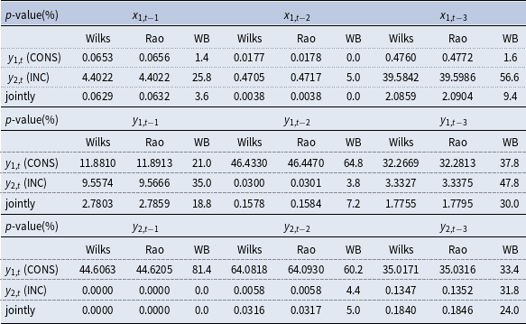
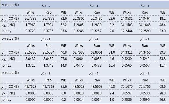
We begin by fitting a VAR model to the series and testing linearity of the two equations against the VLSTR model. We treat lags of both variables and exogeneous variable as potential transition variables. VAR model with four lags (we tried the VAR models up to lag eight and up to four are significant) gives significant parameters for
 $y_{1,t-4}$
, and
 $y_{2,t-4}$
. Thus, we begin with VAR(4) model. We report, hereafter, the main results of the linear VAR model and we point to significant and positive effect of CSI on both consumption and income.

Subsequently, linearity of the VAR model is tested equation by equation. For both equations, we test linearity using the transition variables
 $x_{1,t-d},d=1,2,3,y_{1,t-d},d=1,2,3,$
and
 $y_{2,t-d}, d=1,2,3.$
The below three tables report the results of the linearity tests (Table 2). The
 $p$
-values (multiplied by 100) of regular Wilks’s
 $\Lambda$
test, Rao’s test and wild bootstrapped LM test are reported. LM test and Wilks’s
 $\Lambda$
test produce almost identical results, whereas the wild bootstrap tests perform differently for some equations comparing to the other two tests. The presence of heteroskedasticity might explain the varying performance of the tests.
P-values of no serial correlation tests, parameter constancy tests, and no additive nonlinearity tests

Note: Wilks denotes Wilks’s statistics. Rao denotes Rao’s statistics and WB denotes wild bootstrapping. The sample size of the wild bootstrapping is 500. Note that all of the
 $p$
-values are multiplied by 100 and here read percent.
Overall, linearity is rejected significantly. From the nonlinearity test results, we choose the transition variables according to the
 $p$
-values of the wild bootstrap tests. Thus, we select
 $x_{1,t-2}$
as the optimal transition variable for equation CONS (
 $y_{1,t}),$
and
 $y_{2,t-1}$
as the optimal transition variable for equation INC (
 $y_{2,t}$
). We estimate a 2-regime VLSTR(4) model. Then, we conduct the misspecification test of no-additive nonlinearity and find that the consumption equation still has possible nonlinear additive term, which is controlled by the transition variable
 $x_{1,t-1}$
, whereas there seems no other possible nonlinear term in the income equation. Therefore, we choose
 $x_{1,t-1}$
as the transition variable for equation CONS (
 $y_{1,t}),$
 $y_{2,t-1}$
as the trasition variable for equation INC (
 $y_{2,t}$
), estimate a 2-regime VLSTR(4) model and the obtained estimation results correspond to:

We found that the consumption sentiment has a positive and significant impact on both consumption expenditure and income, while its impact turns to negative in the upper regime. However, the global effect remains positive, which is consistent with the irrational exuberance theory of Shiller and the main findings related to beahvioural finance suggesting that consumer sentiment and confidence might drive the dynamics of consumption. This result is relevant and it is consistent with the related habit consumption theories and the Keynesian approach for which the consumption decision is consistent with the consumer fundamental psychology.
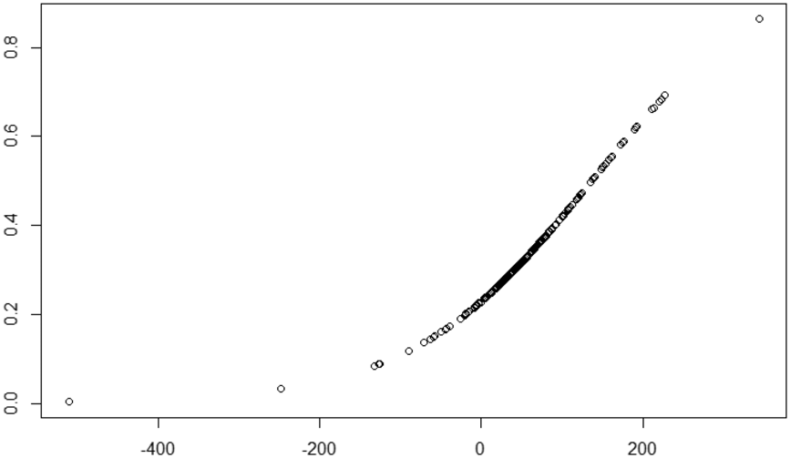
To more accurately visualise these regimes and nonlinearity that characterise the consumption-income relationship, we reported in Figures 1 and 2 the estimated transition function.
Figures 1 and 2 provide the transition functions for the consumption expenditure (CONS) equation and household’s disposable income (INC) equation with the exogeneous variable
 $x_{1t}$
consumer sentiment index (CSI). The top one is the first transition driven by
 $y_{1,t-1}$
in the consumption equation and the bottom one is the transition driven by
 $y_{2,t-1}$
in the income equation. Both graphs show further evidence of different consumption and income regimes confirming the instability of consumption-income relationship. While two distinct consumption regimes appear (low versus high regimes), the transition between these extreme regimes is carried out smoothly reflecting the effect of data aggregation and consumer’s heterogeneity for which the transition between regimes is conducted by changes in consumer sentiment.
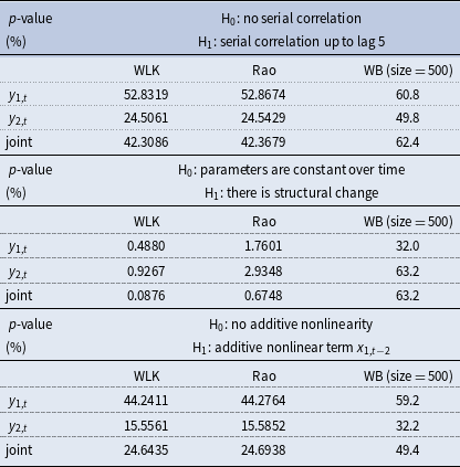
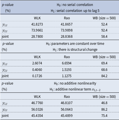
The above model is evaluated by series of misspecification tests including error serial correlation test, parameter constancy test and no-additive nonlinearity test (to INC with lag 2). The results are listed in the below tables. The bootstrapping size is 500.
Overall, the analysis of these misspecification tests show that the above VLSTAR can pass all the evaluation tests, suggesting that our nonlinear model specification is well-specified (See Table 3).
3.2.2 Case 2: federal funds effective rate (FFER) is the exogeneous variable
We begin by fitting a VAR model to the series. VAR model with lag four (we tried the VAR models up to lag eight and up to four are significant) gives significant parameters for
 $y_{1,t-4}$
, and
 $y_{2,t-4}$
. Thus, we start from the following VAR(4) model. Accordingly, the FFER shows a negative and significant effect only on consumption expenditure.

Subsequently, linearity of the VAR model is tested equation by equation. For both equations, we test using the transition variables
 $x_{1,t-d},d=1,2,3,y_{1,t-d},d=1,2,3,$
and
 $y_{2,t-d},d=1,2,3.$
The below three tables report results of the linearity tests. The
 $p$
-values (multiplied by 100) of regular Wilks’s
 $\Lambda$
test, Rao’s test and wild bootstrapped LM test are reported. LM test and Wilks’s
 $\Lambda$
test produce almost identical results, whereas the wild bootstrap tests also perform differently for some equations comparing to the other two, which can be due to further heteroskedasticity in the data.
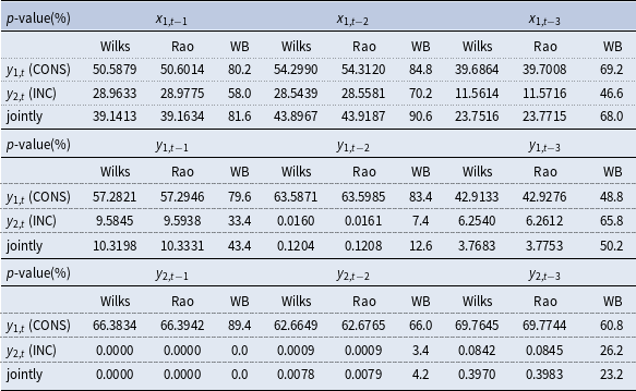
From the nonlinearity test results (mainly based on Bootstrapping, see Yang (Reference Yang2012) for more details) reported in Table 4, we choose no transition variable for equation CONS (
 $y_{1,t}),$
and we select
 $y_{2,t-1}$
as the transition variable for equation INC (
 $y_{2,t}$
). Then, we estimate a 2-regime VLSTR(4) model and we report the main estimation results hereafter. Accordingly, the nonlinearity in the consumption dynamics seems less pronounced with this specification (case 2) than for case 1.
 $P$
-values of linearity tests for the VAR(4) model against the vector logistic smooth transition regression model


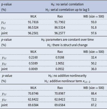
We then run the evaluation tests for error serial correlation, constant parameter over time and no additive nonlinearity (to INC with lag 2). The results are listed in the below tables. The bootstrapping size is 500.
From Table 5, it appears that the above model can pass all the evaluation test.
P-values of no serial correlation tests, parameter constancy tests, and no additive nonlinearity tests

3.2.3 Case 3: net financial wealth (NFW) is the exogeneous variable
We begin by fitting a VAR model to the series. VAR model with lag four (we tried the VAR models up to lag eight and up to four are significant) gives significant parameters for
 $y_{1,t-4}$
, and
 $y_{2,t-4}$
. Thus we set up VAR(4) model. Accordingly, we found a positive and significant (but somewhat weak) effect of net financial wealth on consumption expenditure.

Subsequently, linearity of the VAR model is tested equation by equation. For both equations, we test linearity using the transition variables
 $x_{1,t-d},d=1,2,3,y_{1,t-d},d=1,2,3,$
and
 $y_{2,t-d}, d=1,2,3.$
We report the main results of these linearity tests in Table 6. The
 $p$
-values (multiplied by 100) of regular Wilks’s
 $\Lambda$
test, Rao’s test and wild bootstrapped LM test are reported. LM test and Wilks’s
 $\Lambda$
test produce almost identical results, whereas the wild bootstrap tests perform differently for some equations comparing to the other two. The presence of heteroskedasticity might explain the varying performance of the tests.
 $P$
-values of linearity tests for the VAR(4) model against the vector logistic smooth transition regression model

Based on the the above boostrapped nonlinearity test results no transition variable is selected for equation CONS (
 $y_{1,t}).$
 $y_{2,t-1}$
is the transition variable for equation INC (
 $y_{2,t}$
). Then, we estimate a 2-regime VLSTAR(4) model and the estimation results are as follows. Accordingly, we also point to further evidence of nonlinearity only in the dynamics of household income.

Finally, we run the evaluation tests for error serial correlation, constant parameter over time and no additive nonlinearity (to INC with lag 2). The bootstrapping size is 500. From the results listed in Table 7, it appears that the above model can also pass all the evaluation test.
P-values of no serial correlation tests, parameter constancy tests, and no additive nonlinearity tests

Overall, our findings show different interesting results. First, the VLSTR framework seems suitable enough to reproduce the dynamics of consumption expenditure and household’s income, and it offers the possibility to allow the dynamics of these variables to vary according to the regime and state of the economy. Interestingly, even modelled in a system, following the methodology of Yang (Reference Yang2012) and Teräsvirta and Yang (Reference Teräsvirta and Yang2014), it is not required to impose nonlinearity on both equations. This flexibility is one of the main advantages of VLSTR model and it is relevant to allow the econometrician to model the dynamics of the variable taking the results of linearity test (equation by equation). Second, while the dynamics of household’s income shows further evidence of nonlinearity and regime-switching whatever the VLSTR specification (Case1, Case 2 and Case 3), the dynamics of consumption expenditure exhibits non-linearity only when the consumer sentiment index is considered as an exogenous variable. This result is interesting and suggests that nonlinearity is induced through this information related to a psychological factor: consumer sentiment. While the US consumption dynamics is driven by household’s income and habit formation (as in Jawadi, Reference Jawadi2008; Jawadi and Léoni, Reference Jawadi and Léoni2012), consumer sentiment appears as a fundamental driver for consumption expenditure. Indeed, not only consumer sentiment impacts consumption differently and asymmetrically according to the regime under consideration, lagged consumer sentiment corresponds to the optimal transition variable that activates the transition between consumption expenditure regimes in the US. This finding is particularly relevant to improve the modelling and forecasting of consumption expenditure.
To forecast the future household consumption dynamics, firms, policymakers, and central bankers should closely monitor consumer sentiment as changes in consumer sentiment might signal and indicate the evolution of future consumption. Consumer sentiment is a key driver of regime switching between household consumption states. Furthermore, the VLSTR model appears to supplant the linear model to reproduce the instable and nonlinear consumption_income relationship and this framework can be recommended to model the dynamics of other macroeconomic aggregates.
4. Conclusion
This study investigates the dynamics of household consumption in the US using a nonlinear multivariate framework that allows the household consumption and its drivers to interact asymmetrically and nonlinearly. In addition to including the usual drivers (income, wealth, and interest rates), we develop a time-varying specification that also considers behavioural factors to explain changes in consumption expenditure. This nonlinear multivariate econometric framework offers enough flexibility to capture and reproduce the dynamics of household consumption.
Our analysis yields two interesting results. First, both key economic variables (income, financial wealth, and interest rate) and behavioural factors (consumer sentiment) drive consumer decisions and explain changes in consumption. Second, we show evidence of nonlinearity, asymmetry and switching regimes in consumption and income dynamics. Interestingly, while the dynamics of household income exhibit nonlinear behaviour irrespective of the driver, the nonlinearity in household consumption becomes more pronounced when considering changes in consumer sentiment. This result is particularly relevant as it suggests that considering nonlinearity in a multivariate framework driven by consumer sentiment improves the understanding of changes in consumption decisions. This finding is particularly relevant for consumers, producers, and policymakers to more accurately forecast changes in consumer behaviour. Focusing on the evolution of consumer sentiment would better help to forecast a further change or switching in household consumption. A future extension of this study would be to rely on our VLSTR model to provide out-of-sample forecasts. Furthermore, the VLSTR model appears supplanting linear VAR model and it would be recommended to be applied to model the dynamics of other macroeconomic aggregates.
Competing interests
None
Appendix: Estimated Transition Functions
Transition fuction of Equation (1) -Case 1.

Transition fuction of Equation (2) -Case 1.Footnote 1