1 Introduction
The number of recent contributions aimed at describing the disintegration of liquid jets in air is a natural consequence of the relevance of drop and fibre generation processes in many different technological applications, such as ink-jet printing, catalysis, atomization or combustion (Loscertales et al. Reference Loscertales, Barrero, Márquez, Spretz, Velarde-Ortiz and Larsen2004; Eggers & Villermaux Reference Eggers and Villermaux2008; Basaran, Gao & Bhat Reference Basaran, Gao and Bhat2013). New biotechnological, pharmaceutical, medical or environmental applications demand, however, the controlled generation of micrometre-sized simple or compound drops within another immiscible liquid for their use as biological microreactors, as drug carriers (Barrero & Loscertales Reference Barrero and Loscertales2007) or as building blocks of new materials (Fernández-Nieves et al. Reference Fernández-Nieves, Vitelli, Utada, Link, Márquez, Nelson and Weitz2007; Lopez-Leon et al. Reference Lopez-Leon, Koning, Devaiah, Vitelli and Fernández-Nieves2011). In conventional emulsification methods, the uncontrolled fluctuating shear stresses created either by mechanical agitation or by the turbulent flow of the continuous phase (Garti Reference Garti1997; Rodríguez-Rodríguez, Gordillo & Martínez-Bazán Reference Rodríguez-Rodríguez, Gordillo and Martínez-Bazán2006) lead to the formation of emulsions consisting of simple or compound drops with a large size dispersion (Chong et al. Reference Chong, Liu, Ma, Huang, Han, Cui, Yan and Xu2015). New applications require, however, the generation of monodisperse simple or complex emulsions composed of drops of controllable diameters (Shah et al. Reference Shah, Shum, Rowat, Lee, Agresti, Utada, Chu, Kim, Fernández-Nieves and Martinez2008; Zarzar et al. Reference Zarzar, Sresht, Sletten, Kalow, Blankschtein and Swager2015), and it is our purpose here to provide a detailed experimental and theoretical description of the generation of simple and compound jets and drops within another immiscible liquid under well-controlled and realistic operating conditions.
The capability of microfluidics to produce drops of controllable size (Thorsen et al. Reference Thorsen, Roberts, Arnold and Quake2001) has triggered the emergence of a myriad of different emulsification techniques with different geometrical arrangements but based on very similar physical principles. A few of these techniques rely on the use of electrical stresses to stretch and accelerate a stream of a conducting liquid for its subsequent disintegration into droplets in air (see e.g. de la Mora Reference de la Mora2007; Collins et al. Reference Collins, Sambath, Harris and Basaran2013) and within an insulator liquid bath (see e.g. Loscertales et al. Reference Loscertales, Barrero, Guerrero, Cortijo, Márquez and Gañán Calvo2002; Marín et al. Reference Marín, Loscertales, Márquez and Barrero2007). Nevertheless, most of the new emulsification methods make use of stresses of hydrodynamic origin to force the production of droplets in poly(dimethylsiloxane) (PDMS) microchannels. For instance, in Garstecki et al. (Reference Garstecki, Fuerstman, Stone and Whitesides2006), monodisperse simple microemulsions are generated by means of a cross-flow at the junction of two perpendicular microchannels, whereas Anna, Bontoux & Stone (Reference Anna, Bontoux and Stone2003) report the generation of micrometre-sized drops using a two-dimensional flow focusing type of geometry. Simple and double monodisperse emulsions composed of drops of controllable size can also be produced in glass capillaries, as originally reported by Utada et al. (Reference Utada, Lorenceau, Link, Kaplan, Stone and Weitz2005, Reference Utada, Fernández-Nieves, Stone and Weitz2007) and Oh et al. (Reference Oh, Kim, Baek, Seong and Lee2006) and more recently by Nabavi et al. (Reference Nabavi, Vladisavljević, Gu and Ekanem2015). A common feature of all the methods enumerated above is that the high production frequencies usually needed in applications require the production of drops in the so-called jetting regime, i.e. drops form as a result of the growth of capillary instabilities convected downstream of either simple or compound microjets flowing within an immiscible carrier liquid (Utada et al. Reference Utada, Fernández-Nieves, Gordillo and Weitz2008; Herrada et al. Reference Herrada, Montanero, Ferrera and Gañán Calvo2010).
The capillary stability of a cylindrical liquid jet immersed into another immiscible liquid was previously studied by Tomotika (Reference Tomotika1935), whereas the stability analysis corresponding to the analogous case of compound liquid jets was performed by Sanz & Meseguer (Reference Sanz and Meseguer1985) and Chauhan et al. (Reference Chauhan, Maldarelli, Papageorgiou and Rumschitzki2000). Chauhan et al. (Reference Chauhan, Maldarelli, Papageorgiou and Rumschitzki2000) reported the existence of two different unstable capillary modes and showed that, under the vast majority of conditions, the growth rate of the mode for which the two interfaces grow in phase is larger than the corresponding growth rate of the mode where the two interfaces grow out of phase. This finding, which was later confirmed by means of nonlinear numerical simulations by Suryo, Doshi & Basaran (Reference Suryo, Doshi and Basaran2006) and Vu et al. (Reference Vu, Homma, Tryggvason, Wells and Takakura2013), indicates that most system conditions promote the generation of compound drops, a result in accordance with the experimental fact that the capillary breakup of a compound jet within another immiscible liquid constitutes a feasible and practicable method for the controlled generation of double emulsions. Moreover, Chauhan et al. (Reference Chauhan, Maldarelli, Papageorgiou and Rumschitzki2000) also found that the differences between the growth rates of the two different unstable modes identified become even larger for decreasing thicknesses of the annulus surrounding the inner jet. Interestingly enough, Chauhan et al. (Reference Chauhan, Maldarelli, Papageorgiou and Rumschitzki2000) also reported that, in the limit of thin liquid annuli, the compound jet behaves as a single jet with the interfacial tension coefficient resulting from the addition of the two tensions.
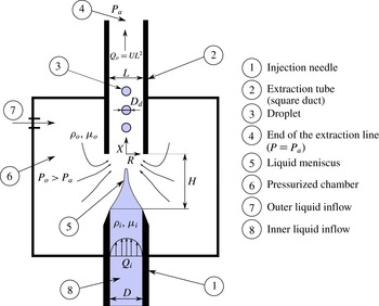
As pointed out above, many different microfluidic devices have been designed with the purpose of generating, in a controlled manner, simple or double microemulsions at production frequencies exceeding 5 kHz by means of the capillary breakup of simple or compound jets flowing into another immiscible liquid. However, the progress made in the experimental (Hertz & Hermanrud Reference Hertz and Hermanrud1983) and analytical description of the dynamics of such types of microjets is still far from being comparable to the advances accomplished in the analysis of the analogous case of liquid jets in air (Eggers & Dupont Reference Eggers and Dupont1994; García & Castellanos Reference García and Castellanos1994; Ambravaneswaran et al. Reference Ambravaneswaran, Subramani, Philips and Basaran2004; Guerrero, González & García Reference Guerrero, González and García2012; Rubio-Rubio, Sevilla & Gordillo Reference Rubio-Rubio, Sevilla and Gordillo2013; Driessen et al. Reference Driessen, Sleutel, Dijksman, Jeurissen and Lohse2014). Motivated by the potential applications of simple and double microemulsions, in this contribution we will analyse, from both experimental and theoretical points of view, the dynamics of long liquid jets breaking into droplets of very similar size within an outer stream of another immiscible liquid. More precisely, it is our purpose here to extend the analytical framework developed in Castro-Hernández, Campo-Cortés & Gordillo (Reference Castro-Hernández, Campo-Cortés and Gordillo2012) and Gordillo, Sevilla & Campo-Cortés (Reference Gordillo, Sevilla and Campo-Cortés2014) to describe the generation and subsequent breakup of simple jets when the Reynolds number characterizing the outer flow of liquid is much larger than unity. We will also extend our previous slender-body theory, valid in the Stokes limit, to analyse the dynamics of compound jets under creeping flow conditions. Our analytical results will be checked by comparing the computed shapes with those observed experimentally in a type of set-up, already described in Evangelio, Campo-Cortés & Gordillo (Reference Evangelio, Campo-Cortés and Gordillo2015) and also sketched in figure 1, that shares similarities with both the flow focusing and the selective withdrawal geometries (Gañán Calvo Reference Gañán Calvo1998; Cohen et al. Reference Cohen, Li, Hougland, Mrksich and Nagel2001). Our technique, which will be termed ‘confined selective withdrawal’, allows the flow rates of the different liquids to be controlled with high precision and, most importantly, the resulting simple or compound jet to be visualized in a straightforward manner thanks to the fact that the tubes used in our design are millimetric. Our procedure is conceptually similar to that in Barrero & Loscertales (Reference Barrero and Loscertales2007) and Marín et al. (Reference Marín, Loscertales, Márquez and Barrero2007), where two immiscible fluids issued from two coaxial tubes are stretched by electrical stresses, the only conceptual difference being that, in our case, electrical stresses are substituted by those of hydrodynamic origin. We will focus on the generation of simple and compound drops arising from the capillary breakup of surfactant-free simple or compound stretched microjets (Suryo & Basaran Reference Suryo and Basaran2006; Anna Reference Anna2016).
Sketch of the drop production device operating in the regime of interest for applications, in which drops with very similar diameters
 $D_{d}$
are produced. Drops are regularly emitted from the tip of a steady and highly stretched liquid ligament attached at the exit of the injection needle. The origin of the dimensionless coordinate
 $x=X/L$
is located at the entrance of the square duct. The imposed inner liquid flow rate is
 $Q_{i}$
and the outer liquid flow rate is
 $UL^{2}$
.

The paper is structured as follows. In § 2, we present the phenomenological description of the jet and drop formation processes under those conditions for which the Reynolds number characterizing the outer coflow,
 $Re_{o}$
, is either large or of order unity or smaller. In § 3, we develop a slender-body approximation to predict the steady shapes of the liquid jets in both the high- and low-Reynolds-number limits; in this section, a comparison with experiments is also provided. In § 4, scalings for the drop formation frequencies and drop diameters are deduced and compared with experiments. In § 5 we determine the values of the critical capillary numbers for steady jets to be formed in the low-Reynolds-number limit. The main results of the paper are summarized in § 6.
2 Phenomenology
In our experimental set-up, sketched in figure 1, a flow rate
 $Q_{o}$
of an outer liquid of density
 $\unicode[STIX]{x1D70C}_{o}$
and viscosity
 $\unicode[STIX]{x1D707}_{o}$
, constituting the continuous phase, flows into a chamber of pressure
 $P_{0}$
larger than atmospheric,
 $P_{a}$
. The fluid(s) to be dispersed enter the reservoir either through a cylindrical tube of inner diameter
 $D_{i}$
or through two coaxial tubes of respective inner diameters
 $D_{i}$
and
 $D_{m}$
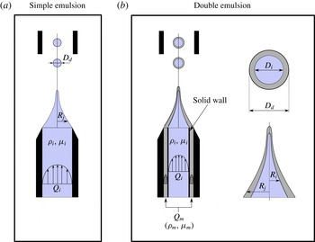
. In the case of generation of simple emulsions, the density, viscosity and flow rate of the liquid to be dispersed will be denoted as
 $\unicode[STIX]{x1D70C}_{i}$
,
 $\unicode[STIX]{x1D707}_{i}$
and
 $Q_{i}$
. Analogously,
 $\unicode[STIX]{x1D70C}_{i,m}$
,
 $\unicode[STIX]{x1D707}_{i,m}$
and
 $Q_{i,m}$
will indicate the material properties and flow rates of the inner (
 $i$
) and middle (
 $m$
) liquids contained in the drops forming the double emulsion (see figure 2). The different liquids involved in the emulsification process flow from the pressurized reservoir towards the atmosphere through a square extraction tube of width
 $L=1$
mm, aligned with the injection tube(s). In our device, the distance
 $H$
separating the exit of the injection tube(s) from the entrance of the extraction tube is not fixed, but can be varied in a range of values. In the case of simple emulsions, the diameter
 $D_{i}$
of the injection tube is also varied in the experimental study, but
 $D_{i}=1000~\unicode[STIX]{x03BC}\text{m}$
and
 $D_{m}=1200~\unicode[STIX]{x03BC}\text{m}$
remain fixed in the case of the generation of complex emulsions. The imposed pressure difference
 $P_{0}-P_{a}$
fixes the mean liquid velocity
 $U$
in the square tube and also generates a pressure gradient from the exit of the injection tube(s) towards the entrance of the extraction duct, favouring the downstream stretching of the simple or compound liquid ligament. The outer liquid flow rate,
 $Q_{o}=UL^{2}$
, is calculated by measuring the volume of liquid exiting the pressurized chamber in a given interval of time, whereas the flow rates
 $Q_{i}$
and
 $Q_{m}$
are controlled using syringe pumps. Images are captured using a Phantom V7 high-speed camera, which, depending on
 $U$
, is operated between 1000 and
 $19\,000~\text{frames}~\text{s}^{-1}$
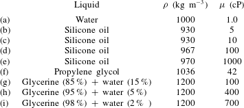
. Table 1 shows the material properties of the different fluids used in the experiments as well as the values of the interfacial tension coefficients corresponding to the different liquid combinations investigated.
(a) Sketch illustrating the generation of simple emulsions. (b) In the case of double emulsions, two liquids with respective flow rates
 $Q_{i}$
(inner liquid) and
 $Q_{m}$
(middle liquid) are injected into the pressurized reservoir from a coaxial injection tube.

Physical properties of the different liquids used in the experiments. The interfacial tension coefficients for the different combinations of immiscible liquids used in the experimental study are as follows: water – silicone oil,
 $\unicode[STIX]{x1D70E}=0.04~\text{N}~\text{m}^{-1}$
; propylene glycol – silicone oil,
 $\unicode[STIX]{x1D70E}=0.01~\text{N}~\text{m}^{-1}$
; glycerine
 $+$
water – silicone oil,
 $\unicode[STIX]{x1D70E}=0.03~\text{N}~\text{m}^{-1}$
. In rows (g)–(i) mass percentages are used. The material properties of the different liquids used in this study have been obtained from the literature.

Owing to the fact that
 $|\unicode[STIX]{x0394}\unicode[STIX]{x1D70C}|gH/(32\unicode[STIX]{x1D707}_{o}U/L)\ll 1$
and
 $|\unicode[STIX]{x0394}\unicode[STIX]{x1D70C}|gH/(\unicode[STIX]{x1D70C}_{o}U^{2})\ll 1$
with
 $\unicode[STIX]{x0394}\unicode[STIX]{x1D70C}=\unicode[STIX]{x1D70C}_{i}-\unicode[STIX]{x1D70C}_{o}$
, the experimental data to be presented in this section are not affected, in a first approximation, by buoyancy effects.
The experimental study is divided into two parts: the generation of simple emulsions within an outer liquid stream with a characteristic Reynolds number that can be set to values either much larger or much smaller than unity; and the generation of double emulsions in a co-flow of a liquid stream dominated by viscosity.
2.1 Simple emulsions
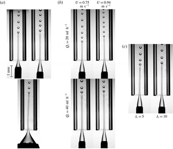
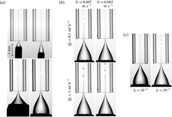
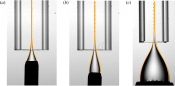
Figure 3 shows the generation process of an oil-in-water (O/W) emulsion by means of the capillary disintegration of a silicone oil jet of diameter
 $2R_{j}(X)$
flowing within a water stream of mean velocity
 $U$
(see also the sketch in figure 1). Owing to the fact that
 $Q_{i}\ll UL^{2}$
, the liquid jet stretches in the downstream direction and, since
 $R_{j}\ll L$
, the diameters of the droplets generated,
 $D_{d}$
, are also noticeably smaller than the width of the extraction tube, i.e.
 $D_{d}\ll L$
. The Reynolds and Weber numbers characterizing the outer flow of liquid,
 $$\begin{eqnarray}\displaystyle Re_{o}=\frac{\unicode[STIX]{x1D70C}_{o}UL}{\unicode[STIX]{x1D707}_{o}},\quad We_{o}=\frac{\unicode[STIX]{x1D70C}_{o}U^{2}(Q_{i}/U)^{1/2}}{\unicode[STIX]{x1D70E}}, & & \displaystyle\end{eqnarray}$$
with
 $(Q_{i}/U)^{1/2}$
the characteristic diameter of the jet are, under all experimental conditions of interest for applications in which the continuous phase is water, such that
 $Re_{o}\sim O(10^{3})$
and
 $We_{o}\gtrsim O(1)$
. Indeed, although not shown here, for values of the Weber number below a threshold value of order unity, a long liquid jet is never formed. Instead, unequal-sized oil droplets of diameters comparable to
 $D_{i}$
are formed at low frequencies right at the injection tube, in agreement with the findings reported in Utada et al. (Reference Utada, Fernández-Nieves, Stone and Weitz2007). From the analysis of the images in figure 3(a), it can be inferred that, although the overall shape of the jets formed depends on the particular values of
 $H$
and
 $D_{i}$
, both the diameter of the jet right upstream of the position where it breaks into drops and
 $D_{d}$
are not sensitive to geometric modifications. This is so because drops are generated from the growth of a capillary instability in a cylindrical jet of characteristic diameter
 $\propto (Q_{i}/U)^{1/2}$
, with
 $U$
the outer liquid velocity at the axis of symmetry of the extraction tube. Interestingly, figure 3(b) shows that the jet diameter at the position where it breaks into drops and
 $D_{d}$
can be reduced either by decreasing
 $Q_{i}$
while keeping
 $U$
constant or by increasing
 $U$
for a given value of
 $Q_{i}$
. Figure 3(c) shows that a twofold increase in liquid viscosity does not have an appreciable effect on the overall shape of the jets or the diameters of the droplets generated. From the images depicted in figure 3, notice that the liquid jet is not perfectly aligned with the axis of the extraction tube. This is due to the fact that, for the values of the Reynolds number characterizing the outer liquid stream
 $Re_{o}\sim 1000$
, the flow is prone to develop Kelvin–Helmholtz instabilities. In addition,
 $Re_{o}\sim 1000$
is close to the critical value for the laminar–turbulent transition of the flow in the extraction tube.
The effect of varying the different parameters governing the generation of O/W simple emulsions (
 $\unicode[STIX]{x1D70E}=0.04~\text{N}~\text{m}^{-1}$
). (a) The effect of varying the diameter
 $D_{i}$
of the injector and of the distance
 $H$
on the drop generation process. Here,
 $U=0.85~\text{m}~\text{s}^{-1}$
,
 $Q_{i}=30~\text{ml}~\text{h}^{-1}$
,
 $\unicode[STIX]{x1D707}_{i}=5~\text{cP}$
,
 $\unicode[STIX]{x1D707}_{o}=1~\text{cP}$
(
 $\unicode[STIX]{x1D706}_{i}=\unicode[STIX]{x1D707}_{i}/\unicode[STIX]{x1D707}_{o}=5$
) and
 $Re_{o}=\unicode[STIX]{x1D70C}_{o}UL/\unicode[STIX]{x1D707}_{o}=850$
. (b) The effects of varying both
 $U$
and
 $Q_{i}$
. Here,
 $\unicode[STIX]{x1D707}_{i}=5~\text{cP}$
,
 $\unicode[STIX]{x1D707}_{o}=1~\text{cP}$
(
 $\unicode[STIX]{x1D706}_{i}=5$
),
 $Re_{o}=750$
(left) and
 $Re_{o}=940$
(right). (c) For a fixed value of the flow-rate ratio,
 $q_{i}=Q_{i}/(UL^{2})=0.011$
, the images show the effect of varying the inner fluid viscosity for a value of the outer Reynolds number
 $Re_{o}=940$
. In all images,
 $D_{i}=0.45$
mm, except at the bottom of panel (a), where
 $D_{i}=1.38$
mm. In all images,
 $H=0.95$
mm, except in the top left image of panel (a), where
 $H=0.45$
mm, and in the bottom image of panel (a), where
 $H=1.1$
mm.

Figure 4 shows the generation of water-in-oil (W/O) emulsions by means of the capillary disintegration of a water jet flowing within an outer stream of a silicone oil with a viscosity of either
 $\unicode[STIX]{x1D707}_{o}=100$
cP or
 $\unicode[STIX]{x1D707}_{o}=1000$
cP and
 $Q_{i}\ll UL^{2}$
. Similarly to the case of O/W emulsions illustrated in figure 3, the overall shape of the jet is sensitive to variations of
 $D_{i}$
and
 $H$
, while the diameters of the droplets generated can be reduced or increased by varying
 $Q_{i}$
and
 $U$
. This is so because drops are generated from the growth of a capillary instability in a cylindrical jet of characteristic diameter
 $\propto [Q_{i}/(2U)]^{1/2}$
, with
 $2U$
the outer liquid velocity at the axis of symmetry of the extraction tube when
 $Re_{o}\lesssim O(1)$
. However, in this case, the stretched liquid jet is aligned with the axis of the extraction tube and, moreover, the drop production process is remarkably periodic: indeed, notice from the images in figure 4 that the diameters of the drops formed, as well as the distances between two neighbouring drops, are constant for fixed values of
 $Q_{i}$
and
 $U$
. Figure 4(c) shows that, in the present case, the diameters of the drops and the distances between them are sensitive to modifications of the outer liquid viscosity. The differences observed with the process of generation of O/W emulsions depicted in figure 3 are due to the fact that, in the case of figure 4, the characteristic Reynolds number is such that
 $Re_{o}\lesssim O(1)$
. Moreover, in this case, the outer capillary number, defined as
 $$\begin{eqnarray}\displaystyle Ca_{o}=\frac{\unicode[STIX]{x1D707}_{o}U}{\unicode[STIX]{x1D70E}}, & & \displaystyle\end{eqnarray}$$
is above a threshold value
 $Ca^{\ast }\sim O(1)$
below which the frequency of drop production is not constant and, consequently, the diameters of the droplets composing the emulsion are not uniform (Gordillo et al.
Reference Gordillo, Sevilla and Campo-Cortés2014).
The effect of varying the different parameters governing the generation of W/O emulsions (
 $\unicode[STIX]{x1D70E}=0.04~\text{N}~\text{m}^{-1}$
). (a) The effect of varying the diameter
 $D_{i}$
of the injector and the distance
 $H$
on the drop generation process. Here,
 $U=0.275~\text{m}~\text{s}^{-1}$
,
 $Q_{i}=1~\text{ml}~\text{h}^{-1}$
,
 $\unicode[STIX]{x1D707}_{i}=1~\text{cP}$
,
 $\unicode[STIX]{x1D707}_{o}=100~\text{cP}$
(
 $\unicode[STIX]{x1D706}_{i}=\unicode[STIX]{x1D707}_{i}/\unicode[STIX]{x1D707}_{o}=0.01$
) and
 $Re_{o}=2.65$
. (b) The effects of varying both
 $U$
and
 $Q_{i}$
. Here,
 $\unicode[STIX]{x1D707}_{i}=1~\text{cP}$
,
 $\unicode[STIX]{x1D707}_{o}=1000~\text{cP}$
(
 $\unicode[STIX]{x1D706}_{i}=0.001$
),
 $Re_{o}=0.045$
(left) and
 $Re_{o}=0.06$
(right). (c) For a fixed value of the flow-rate ratio,
 $q_{i}=Q_{i}/(UL^{2})=0.001$
, the images show the effect of varying the viscosity of the outer fluid. Here,
 $Re_{o}=2.09$
(left) and
 $Re_{o}=0.05$
(right). In all images,
 $D_{i}=1.38$
mm, except in the top images of panel (a), where
 $D_{i}=0.45$
mm. In all images,
 $H=1.85$
mm, except in the top left image of panel (a), where
 $H=0.45$
mm, and in the top right and bottom left images of panel (a), where
 $H=0.95$
mm.

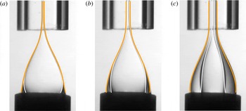
The effect of varying the different parameters governing the generation of double emulsions. (a) The effect of varying the distance of the injector to the extraction tube when the middle fluid is propylene glycol and both the inner liquid and the continuous phase are silicone oils. Therefore,
 $\unicode[STIX]{x1D70E}_{i,m}=0.01~\text{N}~\text{m}^{-1}$
, with
 $\unicode[STIX]{x1D70E}_{i}$
the interfacial tension coefficient between the inner and middle fluids and
 $\unicode[STIX]{x1D70E}_{m}$
the interfacial tension coefficient between the middle fluid and the continuous phase. Here,
 $\unicode[STIX]{x1D707}_{i}=10~\text{cP}$
,
 $\unicode[STIX]{x1D707}_{m}=42~\text{cP}$
,
 $\unicode[STIX]{x1D707}_{o}=1000~\text{cP}$
,
 $U=0.02~\text{m}~\text{s}^{-1}$
,
 $Q_{i}=0.5~\text{ml}~\text{h}^{-1}$
,
 $Q_{m}=0.5~\text{ml}~\text{h}^{-1}$
and, consequently,
 $q=(Q_{i}+Q_{m})/(UL^{2})=0.014$
and
 $Re_{o}=0.02$
. (b) The effects of varying both the outer fluid velocity and the total flow rate
 $Q=Q_{i}+Q_{m}$
on the generation of compound drops. In this case, the middle liquid is propylene glycol and both the inner fluid and the continuous phase are different silicone oils:
 $\unicode[STIX]{x1D70E}_{i,m}=0.01~\text{N}~\text{m}^{-1}$
,
 $\unicode[STIX]{x1D707}_{i}=5~\text{cP}$
,
 $\unicode[STIX]{x1D707}_{m}=42~\text{cP}$
,
 $\unicode[STIX]{x1D707}_{o}=1000~\text{cP}$
,
 $Re_{o}=0.015$
(left) and
 $Re_{o}=0.02$
(right). (c) The effect of varying the middle liquid viscosity on the generation of compound drops. In this case, the middle liquid is a mixture of glycerine
 $+$
water in two different proportions, while the inner liquid as well as the continuous phase are silicone oils of viscosities
 $\unicode[STIX]{x1D707}_{i}=10~\text{cP}$
and
 $\unicode[STIX]{x1D707}_{o}=1000~\text{cP}$
, respectively, and
 $\unicode[STIX]{x1D70E}_{i,m}=0.03~\text{N}~\text{m}^{-1}$
. Left:
 $U=0.045~\text{m}~\text{s}^{-1}$
,
 $Q_{i}=1~\text{ml}~\text{h}^{-1}$
,
 $Q_{m}=2~\text{ml}~\text{h}^{-1}$
,
 $\unicode[STIX]{x1D706}_{i}=0.01$
,
 $\unicode[STIX]{x1D706}_{m}=\unicode[STIX]{x1D707}_{m}/\unicode[STIX]{x1D707}_{o}=0.1$
and
 $Re_{o}=0.043$
. Right:
 $U=0.045~\text{m}~\text{s}^{-1}$
,
 $Q_{i}=2~\text{ml}~\text{h}^{-1}$
,
 $Q_{m}=1~\text{ml}~\text{h}^{-1}$
,
 $\unicode[STIX]{x1D706}_{i}=0.01$
,
 $\unicode[STIX]{x1D706}_{m}=0.4$
and
 $Re_{o}=0.043$
. In these experiments, the ratio
 $q=(Q_{i}+Q_{m})/(UL^{2})$
is kept constant. (d) The effect of varying the inner fluid viscosity on the generation of compound drops. In this case, the middle liquid is propylene glycol,
 $\unicode[STIX]{x1D707}_{m}=42~\text{cP}$
, and the inner fluid and the continuous phase are silicone oils. The outer fluid viscosity is kept constant at
 $\unicode[STIX]{x1D707}_{o}=1000~\text{cP}$
; therefore,
 $\unicode[STIX]{x1D706}_{m}=0.042$
and
 $\unicode[STIX]{x1D70E}_{i,m}=0.01~\text{N}~\text{m}^{-1}$
. Left:
 $U=0.014~\text{m}~\text{s}^{-1}$
,
 $Q_{i}=0.3~\text{ml}~\text{h}^{-1}$
,
 $Q_{m}=0.3~\text{ml}~\text{h}^{-1}$
,
 $\unicode[STIX]{x1D707}_{i}=5~\text{cP}$
,
 $\unicode[STIX]{x1D706}_{i}=5\times 10^{-3}$
and
 $Re_{o}=0.013$
. Right:
 $U=0.025~\text{m}~\text{s}^{-1}$
,
 $Q_{i}=0.5~\text{ml}~\text{h}^{-1}$
,
 $Q_{m}=0.5~\text{ml}~\text{h}^{-1}$
,
 $\unicode[STIX]{x1D707}_{i}=10~\text{cP}$
,
 $\unicode[STIX]{x1D706}_{i}=10^{-2}$
and
 $Re_{o}=0.024$
. In these experiments, the ratio
 $q=(Q_{i}+Q_{m})/(UL^{2})$
is kept constant. In all cases,
 $H=1.75$
mm, except in the left image in panel (a), where
 $H=0.9$
mm. In all cases,
 $D_{i}=1$
mm and
 $D_{m}=1.2$
mm.

2.2 Double emulsions
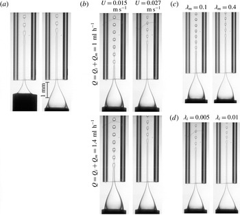
Figure 5 shows the generation of double emulsions consisting of drops containing two immiscible liquids, the inner one being silicone oil and the middle one either propylene glycol or a glycerine plus water mixture. The middle liquid is immiscible with the continuous phase, which, in all the cases considered, is a silicone oil of viscosity
 $\unicode[STIX]{x1D707}_{o}=1000$
cP. The process of generation of the double emulsion also relies upon the capillary breakup of a compound stretched jet aligned with the axis of the extraction tube. Figure 5 shows that, in all cases considered, the drops formed by the capillary breakup of the inner liquid in the compound jet are always encapsulated by the middle liquid surrounding it. The stretched jet is formed after injecting the two liquid flow rates
 $Q_{i}$
and
 $Q_{m}$
(see figure 2) within an outer co-flow of mean velocity
 $U$
satisfying the conditions
 $Q_{i,m}\ll UL^{2}$
,
 $Re_{o}\lesssim O(1)$
and
 $$\begin{eqnarray}\displaystyle Ca_{o}^{\prime }=\frac{\unicode[STIX]{x1D707}_{o}U}{(\unicode[STIX]{x1D70E}_{i}+\unicode[STIX]{x1D70E}_{m})}>Ca^{\ast }\left(\unicode[STIX]{x1D706}_{i},\frac{Q_{i}}{UL^{2}}\right), & & \displaystyle\end{eqnarray}$$
with
 $\unicode[STIX]{x1D706}_{i}=\unicode[STIX]{x1D707}_{i}/\unicode[STIX]{x1D707}_{o}$
. In (2.3),
 $\unicode[STIX]{x1D70E}_{i}$
refers to the interfacial tension coefficient between the two liquids in the compound drop and
 $\unicode[STIX]{x1D70E}_{m}$
to the corresponding value between the middle liquid and the continuous phase liquid. Similarly to the cases of generation of simple emulsions depicted in figures 3 and 4, the overall shape of the compound jet is dependent on the value of
 $H$
for fixed values of
 $\unicode[STIX]{x1D707}_{i,m,o}$
,
 $Q_{i}$
,
 $Q_{m}$
and
 $U$
, but the diameter of the compound drops generated is not (see figure 5
a). The diameter of the drops can be modulated, instead, by varying the different flow rates,
 $Q_{i}$
,
 $Q_{m}$
and
 $UL^{2}$
, as shown in figure 5(b). Figure 5(c,d), where the influence of varying either
 $\unicode[STIX]{x1D707}_{i}$
or
 $\unicode[STIX]{x1D707}_{m}$
for fixed values of
 $\unicode[STIX]{x1D707}_{o}$
,
 $U$
,
 $Q_{i}$
and
 $Q_{m}$
is illustrated, shows that the breakup of the compound jet gives rise to the generation of a train of uniformly sized compound drops separated by a constant distance, a fact evidencing that the drop formation frequency is rather constant. Figure 5(c) also shows that tiny satellite drops of the middle fluid with diameters dependent on
 $\unicode[STIX]{x1D707}_{m}$
are also generated.
3 Slender-body theories describing the steady shapes of the liquid ligaments
The purpose of this section is to deduce the equations predicting, in the limits
 $Re_{o}\gg 1$
and
 $Re_{o}\ll 1$
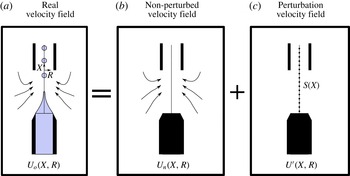
, the steady shapes of the simple or compound jets visualized in figures 3–5 from which drops are produced. The different set of equations describing the downstream evolution of the jet diameter will be based on a one-dimensional description for the flow within the jet and on an extension of the slender-body theory developed in Castro-Hernández et al. (Reference Castro-Hernández, Campo-Cortés and Gordillo2012) and Gordillo et al. (Reference Gordillo, Sevilla and Campo-Cortés2014) describing the flow of the continuous phase. The main idea behind the slender-body approximation is to represent the outer stream as the sum of an unperturbed flow field, calculated numerically using commercial software (ANSYS Fluent), plus the perturbation introduced in the velocity and pressure fields by the presence of the jet. Let us point out here that the theoretical framework to be developed in what follows is applicable to describe axisymmetric flows in which either the inertial or the viscous terms can be neglected in the momentum equation.
Sketches showing that the outer flow field (a) can be decomposed as the addition of two fields: the unperturbed flow field (b), which is calculated numerically using ANSYS Fluent, and the perturbed flow field (c), associated with the presence of the jet. The perturbed velocity field can be quantified as a continuous line of sources of intensity
 $S(X)$
located at the axis of symmetry.

As illustrated in figure 6, the perturbed flow field can be modelled as a continuous distribution of sources with intensities such that the kinematic condition is satisfied at the jet interface. Note that the unperturbed fields are calculated by imposing the impermeability condition at the injection and extraction tubes without including the jet in the numerical simulations (see Evangelio et al. (Reference Evangelio, Campo-Cortés and Gordillo2015) for details). As described in Castro-Hernández et al. (Reference Castro-Hernández, Campo-Cortés and Gordillo2012) and Gordillo et al. (Reference Gordillo, Sevilla and Campo-Cortés2014), one of the advantages of decomposing the flow field as the addition of two fields is the fact that the unperturbed solution depends only on the geometry of the emulsification device. Moreover, since the interface of the liquid jet is close to the axis of symmetry, the only influence of the unperturbed flow field in the one-dimensional equations describing the jet radius appears through the functions
 $U_{xn}(X,R=0)$
and
 $\unicode[STIX]{x2202}^{2}U_{xn}/\unicode[STIX]{x2202}R^{2}(X,R=0)$
. Here,
 $U_{xn}$
denotes the axial velocity of the outer liquid calculated numerically, and the subscript
 $n$
will be used in the following to denote the functions referred to the unperturbed fields. The analysis below will be carried out using variables that are made non-dimensional using
 $U$
and
 $L$
as the characteristic velocity and length scales. From now on, lower-case variables will denote the dimensionless counterparts of the dimensional variables and, consequently,
 $$\begin{eqnarray}\displaystyle x=\frac{X}{L},\quad r=\frac{R}{L},\quad u_{x,r}=\frac{U_{x,r}}{U},\quad h=\frac{H}{L}, & & \displaystyle\end{eqnarray}$$
with the origin of the
 $x$
-coordinate located at the entrance of the extraction tube (see figure 1). The definition of the dimensionless pressure depends on whether the outer flow is dominated by viscous or inertial stresses. More precisely, in the limits
 $Re_{o}\lesssim O(1)$
and
 $Re_{o}\gg 1$
, the dimensionless pressure is respectively defined as
 $$\begin{eqnarray}\displaystyle p=\frac{PL}{\unicode[STIX]{x1D707}_{o}U},\quad p=\frac{P}{\unicode[STIX]{x1D70C}_{o}U^{2}}. & & \displaystyle\end{eqnarray}$$
In the following, the dimensionless outer velocity and pressure fields will be respectively expressed as
 $$\begin{eqnarray}\displaystyle \boldsymbol{u}_{\boldsymbol{o}}=\boldsymbol{u}_{\boldsymbol{n}}+\boldsymbol{u}^{\prime }=[u_{xn}(x,r)+u_{x}^{\prime }]\boldsymbol{e}_{\boldsymbol{x}}+[u_{rn}(x,r)+u_{r}^{\prime }]\boldsymbol{e}_{\boldsymbol{r}},\quad p_{o}=p_{n}+p^{\prime }, & & \displaystyle\end{eqnarray}$$
with
 $\boldsymbol{u}^{\prime }$
and
 $p^{\prime }$
such that
 $|\boldsymbol{u}^{\prime }|\ll \boldsymbol{u}_{\boldsymbol{n}}$
and
 $p^{\prime }\ll p_{n}$
indicating the perturbed velocity and pressure fields. Next, the analytical expression of the outer velocity field in the near-axis region, which is where the jet is located, will be deduced. Note first that the Taylor series expansion of the unperturbed velocity field around
 $r=0$
yields
 $$\begin{eqnarray}\displaystyle \boldsymbol{u}_{\boldsymbol{n}} & = & \displaystyle u_{xn}(x,r)\boldsymbol{e}_{\boldsymbol{x}}+u_{rn}(x,r)\boldsymbol{e}_{\boldsymbol{r}}\nonumber\\ \displaystyle & \simeq & \displaystyle \left[u_{xn}(x,r=0)+\frac{1}{2}\frac{\unicode[STIX]{x2202}^{2}u_{xn}(x,r)}{\unicode[STIX]{x2202}r^{2}}(x,r=0)r^{2}\right]\boldsymbol{e}_{\boldsymbol{x}}+u_{rn}\boldsymbol{e}_{\boldsymbol{r}}\nonumber\\ \displaystyle & = & \displaystyle [u_{x}(x)+f(x)r^{2}]\boldsymbol{e}_{\boldsymbol{x}}+u_{rn}(x,r)\boldsymbol{e}_{\boldsymbol{r}},\end{eqnarray}$$
with
 $u_{x}(x)=u_{xn}(x,r=0)$
and
 $f(x)=(1/2)\,\unicode[STIX]{x2202}^{2}u_{xn}/\unicode[STIX]{x2202}r^{2}(x,r=0)$
. Now, making use of the continuity equation in cylindrical coordinates,
 $\unicode[STIX]{x2202}u_{xn}/\unicode[STIX]{x2202}x+(1/r)\,\unicode[STIX]{x2202}(ru_{rn})/\unicode[STIX]{x2202}r=0$
, we have
 $$\begin{eqnarray}\displaystyle \frac{1}{r}\frac{\unicode[STIX]{x2202}(ru_{rn})}{\unicode[STIX]{x2202}r}=-\frac{\unicode[STIX]{x2202}u_{xn}}{\unicode[STIX]{x2202}x}=-\frac{\text{d}u_{x}}{\text{d}x}-r^{2}\frac{\text{d}^{2}f}{\text{d}x^{2}}\quad \Rightarrow \quad u_{rn}=-\frac{r}{2}\frac{\text{d}u_{x}}{\text{d}x}-\frac{r^{3}}{4}\frac{\text{d}f}{\text{d}x}. & & \displaystyle\end{eqnarray}$$
Consequently, the equation for the near-axis outer velocity field (3.4) can be expressed as
 $$\begin{eqnarray}\displaystyle \boldsymbol{u}_{\boldsymbol{n}}(x,r)=[u_{x}(x)+f(x)r^{2}]\boldsymbol{e}_{\boldsymbol{x}}+\left[-\frac{r}{2}\frac{\text{d}u_{x}}{\text{d}x}(x)-\frac{r^{3}}{4}\frac{\text{d}f}{\text{d}x}(x)\right]\boldsymbol{e}_{\boldsymbol{r}}. & & \displaystyle\end{eqnarray}$$
Since, in the limit
 $Re_{o}\gg 1$
, the axial component of the outer velocity field for
 $r\ll 1$
can be approximated to a plug flow, setting
 $f=0$
in (3.6) yields
 $$\begin{eqnarray}\displaystyle \boldsymbol{u}_{\boldsymbol{n}}(x,r)=u_{x}(x)\boldsymbol{e}_{\boldsymbol{x}}+\left[-\frac{r}{2}\frac{\text{d}u_{x}}{\text{d}x}(x)\right]\boldsymbol{e}_{\boldsymbol{r}}. & & \displaystyle\end{eqnarray}$$
As pointed out in Castro-Hernández et al. (Reference Castro-Hernández, Campo-Cortés and Gordillo2012) and Gordillo et al. (Reference Gordillo, Sevilla and Campo-Cortés2014), the perturbed velocity field can be approximated to that generated by a continuous distribution of sources of intensity
 $s(\bar{x})$
, namely,
 $$\begin{eqnarray}\displaystyle & \displaystyle u_{x}^{\prime }(x,r)=\frac{1}{2}\int _{-h}^{l_{\infty }}\frac{s(\overline{x})(x-\overline{x})}{[(x-\overline{x})^{2}+r^{2}]^{3/2}}\,\text{d}\overline{x}, & \displaystyle\end{eqnarray}$$
 $$\begin{eqnarray}\displaystyle & \displaystyle u_{r}^{\prime }(x,r)=\frac{1}{2}\int _{-h}^{l_{\infty }}\frac{s(\overline{x})r}{[(x-\overline{x})^{2}+r^{2}]^{3/2}}\,\text{d}\overline{x}. & \displaystyle\end{eqnarray}$$
 $u_{r}^{\prime }(x,r)\simeq s(x)/r$
, which is a fairly good approximation to the exact value of
 $u_{r}^{\prime }$
in (3.9) for all values of
 $x$
, except in the region close to the injector,
 $x\simeq -h$
. To improve the agreement between the predicted shapes of the jets and those observed experimentally, the integral (3.9) is approximated here as
 $$\begin{eqnarray}\displaystyle u_{r}^{\prime }(x,r)\simeq -\frac{s(x)}{2r}\left[\frac{x-l_{\infty }}{\sqrt{(x-l_{\infty })^{2}+r^{2}}}-\frac{x+h}{\sqrt{(x+h)^{2}+r^{2}}}\right], & & \displaystyle\end{eqnarray}$$
which is in excellent agreement with the exact value of the integral in (3.9) for all values of
 $x$
.
We checked that (3.8)–(3.10) become independent of
 $l_{\infty }$
for sufficiently high values of this parameter and, consequently, here we have set
 $l_{\infty }=10$
. Let us point out that, while the main contribution of the integral (3.9) was expressed analytically in Castro-Hernández et al. (Reference Castro-Hernández, Campo-Cortés and Gordillo2012) and Gordillo et al. (Reference Gordillo, Sevilla and Campo-Cortés2014), in this contribution the axial and radial components of the perturbed velocity field will be calculated numerically or using the more accurate expression (3.10), respectively. Note now that, making use of the expression for
 $u_{r}^{\prime }(x,r=r_{j})$
given in (3.10), the intensity of the sources can be expressed as a function of the jet radius
 $r_{j}(x)$
by means of the kinematic condition at the jet interface,
 $$\begin{eqnarray}\displaystyle \frac{\text{d}r_{j}(x)}{\text{d}x} & = & \displaystyle \frac{u_{rn}(x,r=r_{j}(x))+u_{r}^{\prime }(x,r=r_{j}(x))}{u_{xn}(x,r=r_{j}(x))+u_{x}^{\prime }(x,r=r_{j}(x))}\nonumber\\ \displaystyle & \simeq & \displaystyle \frac{u_{rn}(x,r=r_{j}(x))+u_{r}^{\prime }(x,r=r_{j}(x))}{u_{xn}(x,r=r_{j}(x))}\quad \nonumber\\ \displaystyle & \Rightarrow & \displaystyle u_{r}^{\prime }(x,r=r_{j}(x))=u_{xn}(x,r=r_{j}(x))\frac{\text{d}r_{j}(x)}{\text{d}x}-u_{rn}(x,r=r_{j}(x))\nonumber\\ \displaystyle & = & \displaystyle [u_{x}(x)+f(x)r_{j}^{2}]\frac{\text{d}r_{j}(x)}{\text{d}x}+\frac{r_{j}}{2}\frac{\text{d}u_{x}(x)}{\text{d}x}+\frac{r_{j}^{3}}{4}\frac{\text{d}f}{\text{d}x}(x).\end{eqnarray}$$
Making use of (3.10) and (3.11) it can be concluded that
 $$\begin{eqnarray}\displaystyle s(x)=-2\frac{[u_{x}(x)+f(x)r_{j}^{2}]r_{j}\displaystyle \frac{\text{d}r_{j}(x)}{\text{d}x}+\frac{r_{j}^{2}}{2}\frac{\text{d}u_{x}(x)}{\text{d}x}+\frac{r_{j}^{4}}{4}\frac{\text{d}f}{\text{d}x}(x)}{\left[\displaystyle \frac{x-l_{\infty }}{\sqrt{(x-l_{\infty })^{2}+r_{j}^{2}}}-\frac{x+h}{\sqrt{(x+h)^{2}+r_{j}^{2}}}\right]}. & & \displaystyle\end{eqnarray}$$
Next, we will make use of the results expressed by (3.8)–(3.11) to deduce the equations describing the downstream evolution of the simple and compound jets in the cases
 $Re_{o}\ll 1$
and
 $Re_{o}\gg 1$
.
3.1 Equations for
 $r_{j}(x)$
and
$r_{i}(x)$
in the limit
$Re_{o}\ll 1$


First of all, let us point out that, since the perturbed velocity field given by (3.8)–(3.10) can be expressed as a function of a velocity potential, the pressure gradient associated with
 $\boldsymbol{u}^{\prime }$
is zero in the Stokes limit (Gordillo et al.
Reference Gordillo, Sevilla and Campo-Cortés2014). Therefore, in the near-axis region
 $r\ll 1$
, the pressure gradient of the outer flow field can be expressed as
 $$\begin{eqnarray}\displaystyle \frac{\unicode[STIX]{x2202}p_{o}}{\unicode[STIX]{x2202}x}(x,r)=\frac{\unicode[STIX]{x2202}p_{n}}{\unicode[STIX]{x2202}x}=\frac{\text{d}^{2}u_{x}}{\text{d}x^{2}}+r^{2}\frac{\text{d}^{2}f}{\text{d}x^{2}}+4f, & & \displaystyle\end{eqnarray}$$
where use has been made of the momentum equation in the limit
 $Re_{o}\rightarrow 0$
(see Gordillo et al. (Reference Gordillo, Sevilla and Campo-Cortés2014) for details). In the case of simple jets, the equation for
 $r_{j}$
is deduced by making use of the continuity equation (Gordillo et al.
Reference Gordillo, Sevilla and Campo-Cortés2014),
 $$\begin{eqnarray}\displaystyle q_{i}=\frac{Q_{i}}{UL^{2}}=[u_{x}(x)+f(x)r_{j}^{2}(x)]\unicode[STIX]{x03C0}r_{j}^{2}(x)-\frac{\unicode[STIX]{x03C0}r_{j}^{4}(x)}{8\unicode[STIX]{x1D706}_{i}}\frac{\text{d}p_{i}(x)}{\text{d}x}. & & \displaystyle\end{eqnarray}$$
In (3.14), the pressure gradient is calculated from the normal stress balance at the jet interface, which, in the limit
 $\unicode[STIX]{x1D707}_{o}\gg \unicode[STIX]{x1D707}_{i}$
, reads
 $$\begin{eqnarray}\displaystyle \frac{\text{d}p_{i}}{\text{d}x}(x,r=r_{j}(x))=\frac{\text{d}p_{n}}{\text{d}x}(x,r=r_{j}(x))+\frac{\text{d}}{\text{d}x}\left[\frac{\unicode[STIX]{x1D712}}{Ca_{o}}-2\left(\frac{\unicode[STIX]{x2202}u_{rn}}{\unicode[STIX]{x2202}r}(r=r_{j})+\frac{\unicode[STIX]{x2202}u_{r}^{\prime }}{\unicode[STIX]{x2202}r}(r=r_{j})\right)\right]. & & \displaystyle \nonumber\\ \displaystyle & & \displaystyle\end{eqnarray}$$
In (3.15),
 $\unicode[STIX]{x2202}u_{rn}/\unicode[STIX]{x2202}r(r=r_{j})=-(1/2)\,\text{d}u_{x}/\text{d}x-(3/4)r_{j}^{2}\,\text{d}f/\text{d}x$
,
 $$\begin{eqnarray}\displaystyle \unicode[STIX]{x1D712}=\unicode[STIX]{x1D735}\boldsymbol{\cdot }\boldsymbol{n}=\frac{1}{r_{j}(1+{\dot{r}}_{j}^{2})^{1/2}}-\frac{\ddot{r}_{j}}{(1+{\dot{r}}_{j}^{2})^{3/2}} & & \displaystyle\end{eqnarray}$$
and dots denote derivatives with respect to
 $x$
. From now on, we will use either
 $\text{d}/\text{d}x$
or a dot to indicate a derivative with respect to
 $x$
. Therefore, the substitution of (3.13) into (3.15) yields
 $$\begin{eqnarray}\displaystyle \frac{\text{d}p_{i}}{\text{d}x}(x,r=r_{j}(x))=\frac{1}{Ca}\frac{\text{d}\unicode[STIX]{x1D712}}{\text{d}x}+2\frac{\text{d}^{2}u_{x}}{\text{d}x^{2}}+4f+3r_{j}\frac{\text{d}r_{j}}{\text{d}x}\frac{\text{d}f}{\text{d}x}+\frac{5}{2}r_{j}^{2}\frac{\text{d}^{2}f}{\text{d}x^{2}}-2\frac{\text{d}}{\text{d}x}\left(\frac{\unicode[STIX]{x2202}u_{r}^{\prime }}{\unicode[STIX]{x2202}r}(r=r_{j})\right) & & \displaystyle \nonumber\\ \displaystyle & & \displaystyle\end{eqnarray}$$
and, once
 $\text{d}p_{i}/\text{d}x$
is expressed as a function of
 $r_{j}(x)$
,
 $u_{x}$
and
 $f$
, the jet radius is calculated by solving the equation
 $$\begin{eqnarray}\displaystyle q_{i} & = & \displaystyle [u_{x}(x)+f(x)r_{j}^{2}(x)]\unicode[STIX]{x03C0}r_{j}^{2}(x)-\frac{\unicode[STIX]{x03C0}r_{j}^{4}(x)}{8\unicode[STIX]{x1D706}_{i}}\left[\frac{1}{Ca}\frac{\text{d}\unicode[STIX]{x1D712}}{\text{d}x}+2\frac{\text{d}^{2}u_{x}}{\text{d}x^{2}}+4f+3r_{j}\frac{\text{d}r_{j}}{\text{d}x}\frac{\text{d}f}{\text{d}x}\right.\nonumber\\ \displaystyle & & \displaystyle +\left.\frac{5}{2}r_{j}^{2}\frac{\text{d}^{2}f}{\text{d}x^{2}}-2\frac{\text{d}}{\text{d}x}\left(\frac{\unicode[STIX]{x2202}u_{r}^{\prime }}{\unicode[STIX]{x2202}r}(r=r_{j})\right)\right],\end{eqnarray}$$
where
 $$\begin{eqnarray}\displaystyle \frac{\unicode[STIX]{x2202}u_{r}^{\prime }}{\unicode[STIX]{x2202}r}(x,r_{j})=\frac{s(x)}{2}\left[\frac{\displaystyle \frac{(x-l_{\infty })^{3}}{r_{j}^{2}}+2(x-l_{\infty })}{[(x-l_{\infty })^{2}+r_{j}^{2}]^{3/2}}-\frac{\displaystyle \frac{(x+h)^{3}}{r_{j}^{2}}+2(x+h)}{[(x+h)^{2}+r_{j}^{2}]^{3/2}}\right] & & \displaystyle\end{eqnarray}$$
is deduced making use of (3.10).
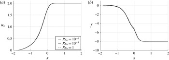
Given the functions
 $u_{x}(x)$
and
 $f(x)$
characterizing a specific geometrical arrangement (see figure 7), the shape of the jet is calculated iteratively: a Newton–Raphson method is used to satisfy (3.18) at discrete collocation points, following a procedure that is quite similar to that described in Gordillo et al. (Reference Gordillo, Sevilla and Campo-Cortés2014), the main difference being that (3.19) needs to be evaluated at the collocation points once the intensity of the sources
 $s(x)$
is calculated as a function of
 $r_{j}$
by means of (3.12). The only boundary condition that needs to be imposed on the system of equations is
 $r_{j}(x=-h)=D_{i}/(2L)$
since the second condition is substituted by the discretized version of the differential equation particularized at the very last node of the numerical domain (see Gordillo et al.
Reference Gordillo, Sevilla and Campo-Cortés2014).
Numerically calculated functions
 $u_{x}$
and
 $f$
in the Stokes limit for the particular case
 $H/L=0.97$
and
 $D/L=0.45$
.

In the analogous case of compound jets, the equations describing the positions of the inner and outer interfaces,
 $r_{i}(x)$
and
 $r_{j}(x)$
respectively (see the sketch in figure 2), are also deduced making use of the continuity equation for each of the two immiscible fluids in the jet, namely,
 $$\begin{eqnarray}\displaystyle q_{i}=\frac{Q_{i}}{UL^{2}}=[u_{x}(x)+f(x)r_{j}^{2}(x)]\unicode[STIX]{x03C0}r_{i}^{2}(x)-\frac{\unicode[STIX]{x03C0}r_{i}^{4}(x)}{8\unicode[STIX]{x1D706}_{i}}\frac{\text{d}p_{i}(x)}{\text{d}x} & & \displaystyle\end{eqnarray}$$
and
 $$\begin{eqnarray}\displaystyle q_{m}=\frac{Q_{m}}{UL^{2}}=[u_{x}(x)+f(x)r_{j}^{2}(x)]\unicode[STIX]{x03C0}(r_{j}(x)^{2}-r_{i}^{2}(x)). & & \displaystyle\end{eqnarray}$$
The validity of neglecting the contribution of the term proportional to the pressure gradient in (3.21) will be checked a posteriori, when the results of the model are compared with the experimental observations. Following the previous derivation, the only remaining step to deduce the differential equations for
 $r_{i}$
and
 $r_{j}$
is to express the pressure gradient
 $\text{d}p_{i}/\text{d}x$
as a function of
 $r_{j}$
. This is done making use of the normal stress balance at the inner interface, which, in the limit
 $\unicode[STIX]{x1D707}_{m}\gg \unicode[STIX]{x1D707}_{i}$
, reads
 $$\begin{eqnarray}\displaystyle p_{i}(x,r=r_{i}(x))=p_{m}(x,r=r_{i}(x))+\frac{\unicode[STIX]{x1D712}_{i}}{Ca_{i}}+\unicode[STIX]{x1D706}_{m}[\dot{u}_{x}(x)+2r_{j}(x){\dot{r}}_{j}(x)f(x)+r_{j}^{2}(x){\dot{f}}(x)], & & \displaystyle \nonumber\\ \displaystyle & & \displaystyle\end{eqnarray}$$
with
 $\unicode[STIX]{x1D706}_{m}=\unicode[STIX]{x1D707}_{m}/\unicode[STIX]{x1D707}_{o}$
and
 $$\begin{eqnarray}\displaystyle \unicode[STIX]{x1D712}_{i}=\frac{1}{r_{i}(1+{\dot{r}}_{i}^{2})^{1/2}}-\frac{\ddot{r}_{i}}{(1+{\dot{r}}_{i}^{2})^{3/2}}. & & \displaystyle\end{eqnarray}$$
In (3.22), the expression for the term proportional to
 $\unicode[STIX]{x1D706}_{m}$
has been deduced consistently with a plug flow type of velocity field for the middle liquid of the form
 $$\begin{eqnarray}\displaystyle \boldsymbol{u}_{\boldsymbol{m}}(x,r)=[u_{x}(x)+f(x)r_{j}^{2}(x)]\boldsymbol{e}_{\boldsymbol{x}}-\frac{r}{2}[\dot{u}_{x}(x)+2r_{j}(x){\dot{r}}_{j}(x)f(x)+r_{j}^{2}(x){\dot{f}}]\boldsymbol{e}_{\boldsymbol{ r}}, & & \displaystyle\end{eqnarray}$$
where use of the continuity equation has been made. In (3.22), the pressure
 $p_{m}$
is deduced from the normal stress balance at the outer interface, which, in the limit
 $\unicode[STIX]{x1D707}_{o}\gg \unicode[STIX]{x1D707}_{m}$
, reads
 $$\begin{eqnarray}\displaystyle p_{m}(x,r=r_{j}(x))=p_{o}(x,r=r_{j}(x))+\frac{\unicode[STIX]{x1D712}}{Ca_{m}}-2\left[\frac{\unicode[STIX]{x2202}u_{rn}}{\unicode[STIX]{x2202}r}(r=r_{j})+\frac{\unicode[STIX]{x2202}u_{r}^{\prime }}{\unicode[STIX]{x2202}r}(r=r_{j})\right], & & \displaystyle\end{eqnarray}$$
with
 $\unicode[STIX]{x1D712}$
given in (3.16).
Therefore, taking the
 $x$
derivative of (3.22) and (3.25), with
 ${\dot{p}}_{o}$
given in (3.13), yields
 $$\begin{eqnarray}\displaystyle {\dot{p}}_{i}(x,r=r_{i}(x)) & = & \displaystyle \frac{\dot{\unicode[STIX]{x1D712}}}{Ca_{m}}+2\ddot{u} _{x}+4f+3r_{j}{\dot{r}}_{j}\,{\dot{f}}+\frac{5}{2}r_{j}^{2}\ddot{f}-2\frac{\text{d}}{\text{d}x}\left(\frac{\unicode[STIX]{x2202}u_{r}^{\prime }}{\unicode[STIX]{x2202}r}(r=r_{j})\right)\nonumber\\ \displaystyle & & \displaystyle +\,\frac{\dot{\unicode[STIX]{x1D712}}_{i}}{Ca_{i}}+\unicode[STIX]{x1D706}_{m}[\ddot{u} _{x}+2{\dot{r}}_{j}^{2}f+2r_{j}\ddot{r}_{j}\,f+4r_{j}{\dot{r}}_{j}\,{\dot{f}}+r_{j}^{2}\ddot{f}],\end{eqnarray}$$
with
 $Ca_{m}=\unicode[STIX]{x1D707}_{o}U/\unicode[STIX]{x1D70E}_{m}$
and
 $Ca_{i}=\unicode[STIX]{x1D707}_{o}U/\unicode[STIX]{x1D70E}_{i}$
.
The substitution of (3.26) into (3.20) yields a system of equations (3.20) and (3.21) for the two unknowns
 $r_{i}$
and
 $r_{j}$
which needs to be complemented with equations (3.12) and (3.19) expressing
 $s(x)$
and
 $\unicode[STIX]{x2202}u_{r}^{\prime }(r=r_{j})/\unicode[STIX]{x2202}r$
as a function of
 $r_{j}$
. The only boundary conditions that need to be imposed on the system of equations are
 $r_{i}(x=-h)=D_{i}/(2L)$
and
 $r_{j}(x=-h)=D_{m}/(2L)$
. Both
 $r_{i}(x)$
and
 $r_{j}(x)$
are also calculated using a Newton–Raphson method: after a few iterations, the method converges and the pair of equations (3.20) and (3.21) are satisfied at discrete collocation points.
The remarkable agreement between the observed and calculated shapes exhibited in figures 8 and 9 confirms that the slender-body theories developed in this section are a powerful tool to predict the shapes of simple and compound jets flowing within another immiscible liquid in realistic experimental situations. The deviations observed in figures 8 and 9 are associated with a slight misalignment between the axes of the injection and extraction tubes. Let us point out that the reason why the model works so well in the vicinity of the injection tube, where the jet interface is not close to the axis of symmetry, is due to the fact that the solution is dominated by the boundary condition at
 $x=-h$
. Moreover, in this region, the dynamical effects of the outer stream are irrelevant, as well as the effect of the precise shape of the velocity profile at the exit of the injection tube.
Simple jets – comparison between the predicted and observed shapes in the case of
 $\unicode[STIX]{x1D706}_{i}=10^{-2}$
for different geometrical arrangements: (a)
 $Ca_{o}=1.04$
,
 $Re_{o}=3.92$
,
 $Q_{i}=0.5~\text{ml}~\text{h}^{-1}$
,
 $U=0.206~\text{m}~\text{s}^{-1}$
; (b)
 $Ca_{o}=1.04$
,
 $Re_{o}=3.92$
,
 $Q_{i}=0.5~\text{ml}~\text{h}^{-1}$
,
 $U=0.21~\text{m}~\text{s}^{-1}$
; (c)
 $Ca_{o}=1.04$
,
 $Re_{o}=3.92$
,
 $Q_{i}=0.5~\text{ml}~\text{h}^{-1}$
,
 $U=0.21~\text{m}~\text{s}^{-1}$
. Notice that the agreement is excellent in spite of the fact that
 $Re_{o}\sim O(1)$
. The agreement is equally good for the cases in which
 $Re_{o}\ll 1$
.

Compound jets – comparison between the predicted and observed shapes for different values of the control parameters when the middle fluid is propylene glycol and the outer fluid viscosity is
 $\unicode[STIX]{x1D707}_{o}=1000~\text{cP}$
: (a)
 $\unicode[STIX]{x1D706}_{m}=0.042$
,
 $\unicode[STIX]{x1D706}_{i}=0.005$
,
 $Ca_{o}^{\prime }=\unicode[STIX]{x1D707}_{o}U/(\unicode[STIX]{x1D70E}_{i}+\unicode[STIX]{x1D70E}_{m})=0.7$
,
 $Re_{o}=0.027$
,
 $Q_{i}=0.1~\text{ml}~\text{h}^{-1}$
,
 $Q_{m}=0.1~\text{ml}~\text{h}^{-1}$
,
 $U=0.014~\text{m}~\text{s}^{-1}$
; (b)
 $\unicode[STIX]{x1D706}_{m}=0.04$
,
 $\unicode[STIX]{x1D706}_{i}=0.005$
,
 $Ca_{o}^{\prime }=0.7$
,
 $Re_{o}=0.027$
,
 $Q_{i}=0.3~\text{ml}~\text{h}^{-1}$
,
 $Q_{m}=0.3~\text{ml}~\text{h}^{-1}$
,
 $U=0.014~\text{m}~\text{s}^{-1}$
; (c)
 $\unicode[STIX]{x1D706}_{m}=0.04$
,
 $\unicode[STIX]{x1D706}_{i}=0.01$
,
 $Ca_{o}^{\prime }=1.79$
,
 $Re_{o}=0.067$
,
 $Q_{i}=1~\text{ml}~\text{h}^{-1}$
,
 $Q_{m}=1~\text{ml}~\text{h}^{-1}$
,
 $U=0.035~\text{m}~\text{s}^{-1}$
.

3.2 Equation for
$r_{j}(x)$
in the limit
$Re_{o}\gg 1$


In contrast to the low-Reynolds-number case considered above, the pressure gradient created by the perturbed velocity field is different from zero when
 $Re_{o}\gg 1$
. Indeed, in the near-axis region, where
 $u_{rn}\simeq -r/2\dot{u}_{x}$
since
 $f=0$
in a plug type of flow, Bernoulli’s equation reads, neglecting the higher-order contribution
 $u_{x}^{\prime 2}\ll u_{x}u_{x}^{\prime }$
,
 $$\begin{eqnarray}\displaystyle p_{\infty }=p_{o}(x)+{\textstyle \frac{1}{2}}\boldsymbol{u}_{\boldsymbol{o}}\boldsymbol{\cdot }\boldsymbol{u}_{\boldsymbol{o}}\simeq p_{o}+{\textstyle \frac{1}{2}}[u_{x}^{2}+2u_{x}u_{x}^{\prime }+(r^{2}/4)\dot{u}_{x}^{2}], & & \displaystyle\end{eqnarray}$$
with
 $u_{x}$
the unperturbed velocity in the limit
 $Re_{o}\gg 1$
at
 $r=0$
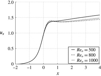
calculated numerically (see figure 10) using ANSYS Fluent. Consequently, at the jet interface
 $r=r_{j}(x)$
,
 $$\begin{eqnarray}\displaystyle {\dot{p}}_{o}=-[u_{x}\dot{u}_{x}+\dot{u}_{x}u_{x}^{\prime }+u_{x}\dot{u}_{x}^{\prime }+(r_{j}^{2}/4)\dot{u}_{x}\ddot{u} _{x}], & & \displaystyle\end{eqnarray}$$
with
 $u_{x}^{\prime }$
calculated using (3.8). The expression for the intensity of the sources deduced from the kinematic boundary condition yields, in the plug flow case
 $f=0$
,
 $$\begin{eqnarray}\displaystyle s(x)=-2\frac{u_{x}(x)r_{j}\displaystyle \frac{\text{d}r_{j}(x)}{\text{d}x}+\displaystyle \frac{r_{j}^{2}}{2}\frac{\text{d}u_{x}(x)}{\text{d}x}}{\left[\displaystyle \frac{x-l_{\infty }}{\sqrt{(x-l_{\infty })^{2}+r_{j}^{2}}}-\displaystyle \frac{x+h}{\sqrt{(x+h)^{2}+r_{j}^{2}}}\right]}. & & \displaystyle\end{eqnarray}$$
In the high-Reynolds-number limit, the continuity equation for the flow of liquid within the jet reads
 $q_{i}=Q_{i}/UL^{2}=\unicode[STIX]{x03C0}ur_{j}^{2}$
and, therefore, the one-dimensional momentum equation deduced in Eggers & Dupont (Reference Eggers and Dupont1994) provides the following equation for
 $r_{j}(x)$
:
 $$\begin{eqnarray}\displaystyle -\frac{2q_{i}^{2}{\dot{r}}_{j}}{\unicode[STIX]{x03C0}^{2}r_{j}^{5}}=-\frac{\unicode[STIX]{x1D70C}_{o}}{\unicode[STIX]{x1D70C}_{i}}\left[{\dot{p}}_{o}+\frac{\unicode[STIX]{x1D70E}}{\unicode[STIX]{x1D70C}_{o}U^{2}L}\dot{\unicode[STIX]{x1D712}}\right]-\frac{6q_{i}}{\unicode[STIX]{x03C0}Re_{o}}\unicode[STIX]{x1D706}_{i}\frac{\ddot{r}_{j}r_{j}-{\dot{r}}_{j}^{2}}{r_{j}^{4}}\frac{\unicode[STIX]{x1D70C}_{o}}{\unicode[STIX]{x1D70C}_{i}}, & & \displaystyle\end{eqnarray}$$
which is solved together with (3.8), (3.16), (3.28) and (3.29) using a Newton–Raphson method. The only boundary condition that needs to be imposed on the system of equations is
 $r_{j}(x=-h)=D_{i}/(2L)$
.
Numerically calculated function
 $u_{x}$
in the high-Reynolds-number limit for the particular case
 $H/L=0.97$
and
 $D/L=0.45$
.

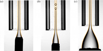
Figure 11 also shows an excellent agreement between the calculated and the experimental shapes, a fact that lends support to the high-Reynolds-number slender-body theory for capillary flows, which, up to our knowledge, has been developed here for the first time. Let us point out that the slight deviations observed in figure 11 are associated to the lateral oscillations of the jet triggered by Kelvin–Helmholtz instabilities.
Comparison between the predicted and observed shapes of steady liquid jets in the case of the generation of oil drops in water, for which
 $Re_{o}\gg 1$
and
 $\unicode[STIX]{x1D70E}=0.04~\text{N}~\text{m}^{-1}$
: in all cases,
 $\unicode[STIX]{x1D706}_{i}=5$
; (a)
 $Q_{i}=40~\text{ml}~\text{h}^{-1}$
,
 $U=0.75~\text{m}~\text{s}^{-1}$
,
 $Re_{o}=755$
; (b)
 $Q_{i}=20~\text{ml}~\text{h}^{-1}$
,
 $U=0.75~\text{m}~\text{s}^{-1}$
,
 $Re_{o}=755$
; (c)
 $Q_{i}=50~\text{ml}~\text{h}^{-1}$
,
 $U=0.85~\text{m}~\text{s}^{-1}$
,
 $Re_{o}=850$
.

4 Scaling the drop diameters and the drop formation frequencies
Assuming that the drop emission process is periodic, the frequency of drop formation
 $f$
can be calculated as the ratio between the velocity at which the tip of the jet is convected downstream of the region where drops are emitted, divided by a length
 $\ell _{0}$
, namely,
 $$\begin{eqnarray}\displaystyle f=\frac{2U}{\ell _{0}}\quad \text{for }Re_{o}\lesssim O(1)\quad \text{and}\quad f=\frac{U}{\ell _{0}}\quad \text{for }Re_{o}\gg 1. & & \displaystyle\end{eqnarray}$$
Notice that, in marked contrast with the process of bubble generation, in which the fragmentation of the gas ligament is forced by the pressure gradient of the outer flow (see Evangelio et al. (Reference Evangelio, Campo-Cortés and Gordillo2015) for details), drops are created in this case as a consequence of the growth of a capillary instability. Consequently,
 $\ell _{0}$
in (4.1) represents the length of the liquid cylinder for which capillary instabilities grow faster. The reason for the factor 2 multiplying
 $U$
in (4.1) is the fact that the maximum velocity of a Poiseuille velocity profile, which is reached where the jet is located, i.e. at the axis of symmetry, is twice the mean velocity.
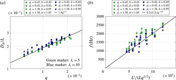
Plots showing that the diameters (a) and frequencies (b) of the oil drops formed in water (
 $Re_{o}\gg 1$
) follow the expected scalings
 $D_{d}\propto Lq^{1/2}$
and
 $f\propto U/(Lq^{1/2})$
, respectively. However, note that the experimental data are rather dispersed with respect to the predicted trends.

Denoting by
 $Q$
the total flow rate of the liquids to be dispersed, i.e.
 $Q=Q_{i}$
in the case of the generation of simple emulsions and
 $Q=Q_{i}+Q_{m}$
in the case of double emulsions, continuity demands that
 $$\begin{eqnarray}\displaystyle \frac{\unicode[STIX]{x03C0}D_{d}^{3}}{6}f=Q, & & \displaystyle\end{eqnarray}$$
with
 $D_{d}$
the outer diameter of the drop. Therefore, making use of (4.1) and (4.2),
 $$\begin{eqnarray}\displaystyle \frac{D_{d}}{L}=\left[\frac{3\ell _{0}/L}{\unicode[STIX]{x03C0}}q\right]^{1/3}\quad \text{for }Re_{o}\lesssim O(1)\quad \text{and}\quad \frac{D_{d}}{L}=\left[\frac{6\ell _{0}/L}{\unicode[STIX]{x03C0}}q\right]^{1/3}\quad \text{for }Re_{o}\gg 1, & & \displaystyle \nonumber\\ \displaystyle & & \displaystyle\end{eqnarray}$$
with
 $q=Q/(UL^{2})$
. Since, in the high-Reynolds-number case, continuity demands that
 $\ell _{0}/L\propto q^{1/2}$
, (4.1) and (4.3) yield
 $f\propto U/(Lq^{1/2})$
and
 $D_{d}/L\propto q^{1/2}$
, these scalings being confirmed in figure 12, where, however, a significant dispersion in the experimental data is observed with respect to the expected trends. The dispersion depicted in figure 12 can be attributed to the lateral fluctuations experienced by the jets in the experiments of the type shown in figure 3, where
 $Re_{o}\sim 10^{3}$
is high enough for Kelvin–Helmholtz non-axisymmetric instabilities to develop and, moreover, these values of the Reynolds number are also near the threshold for which the flow in the extraction tube experiences a laminar–turbulent transition.
In contrast, the production frequency of simple and compound drops is rather constant in the low-Reynolds-number case. This is due to the fact that the highly stretched liquid jets depicted in figures 4 and 5 are steady upstream of the location where the drop production process takes place. Therefore, in the present case, it is worth calculating the wavelength of maximum amplification of capillary waves. For that purpose, we will make use of the dispersion relation,
 $$\begin{eqnarray}\displaystyle D(\unicode[STIX]{x1D714},k) & = & \displaystyle -\text{i}\unicode[STIX]{x1D714}\left(2+\frac{k^{2}}{4\unicode[STIX]{x1D706}_{i}}\right)+\text{i}k\left[2u_{x\infty }+f_{\infty }r_{j\infty }^{2}\left(4-\frac{2}{\unicode[STIX]{x1D706}_{i}}\right)\right]-\frac{k^{2}}{8\unicode[STIX]{x1D706}_{i}Ca}\nonumber\\ \displaystyle & & \displaystyle +\,\text{i}k^{3}\left(\frac{u_{x\infty }}{4\unicode[STIX]{x1D706}_{i}}+\frac{f_{\infty }r_{j\infty }^{2}}{4\unicode[STIX]{x1D706}_{i}}\right)+\frac{k^{4}}{8\unicode[STIX]{x1D706}_{i}Ca}=0,\end{eqnarray}$$
deduced in Gordillo et al. (Reference Gordillo, Sevilla and Campo-Cortés2014) and in appendix A for cylindrical jets and which, in spite of its simplicity, is able to reproduce the results obtained using the much more involved dispersion relation due to Tomotika (Reference Tomotika1935). In (4.4),
 $k$
is a real number and denotes the wavenumber (made dimensionless using the characteristic length
 $R_{j\infty }$
),
 $\unicode[STIX]{x1D714}$
is the complex frequency (made dimensionless using
 $U$
and
 $R_{j\infty }$
as characteristic scales for the velocity and length, respectively),
 $u_{x\infty }=2$
and
 $f_{\infty }=-8$
are the asymptotic values of the functions in figure 7, and
 $r_{j\infty }$
is the solution of the continuity equation,
 $$\begin{eqnarray}\displaystyle q_{i}=[u_{x\infty }+f_{\infty }r_{j\infty }^{2}]\unicode[STIX]{x03C0}r_{j\infty }^{2}-\frac{\unicode[STIX]{x03C0}r_{j\infty }^{4}}{2\unicode[STIX]{x1D706}_{i}}f_{\infty }, & & \displaystyle\end{eqnarray}$$
which is deduced setting to zero all the
 $x$
derivatives in (3.18). Equation (4.5) will also be used in the case of generation of double emulsions: indeed, the reason that the flow-rate ratio
 $q_{i}$
instead of
 $q$
appears in (4.5) is that the capillary breakup of the inner jet triggers the fragmentation of the compound jet. In (4.4),
 $Ca=Ca_{o}^{\prime }=\unicode[STIX]{x1D707}_{o}U/(\unicode[STIX]{x1D70E}_{i}+\unicode[STIX]{x1D70E}_{m})$
in the case of double emulsions, i.e. from the point of view of the stability analysis, a compound jet can be viewed as a simple jet with an effective interfacial tension coefficient
 $\unicode[STIX]{x1D70E}=\unicode[STIX]{x1D70E}_{i}+\unicode[STIX]{x1D70E}_{m}$
, whereas, in the case of simple jets,
 $Ca=Ca_{o}$
.
The dispersion relation (4.4) is used to calculate the wavelength of maximum amplification of capillary disturbances as
 $$\begin{eqnarray}\displaystyle \frac{\ell _{0}}{L}=\frac{2\unicode[STIX]{x03C0}}{k_{max}}r_{j\infty }, & & \displaystyle\end{eqnarray}$$
with
 $k_{max}(Ca,\unicode[STIX]{x1D706}_{i})\in \mathbb{R}$
indicating the wavenumber maximizing the imaginary part of the complex frequency
 $\unicode[STIX]{x1D714}$
in
 $D(\unicode[STIX]{x1D714},k)=0$
.
Once
 $\ell _{0}/L$
is known from the solution of (4.4)–(4.6), both
 $f$
and
 $D_{d}$
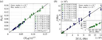
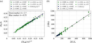
are calculated making use of (4.1) and (4.3). The results obtained, depicted in figures 13 and 14, are in excellent agreement with the experimental measurements. Note also that the dispersion of the experimental data with respect to the expected trends is quite narrow, a fact confirming the periodicity of the drop emission process suggested in figures 4 and 5.
Case of simple emulsions: the diameters (a) and frequencies (b) of the simple emulsions generated when
 $Re_{o}\lesssim O(1)$
follow the expected scalings given in (4.3) and (4.1), respectively, with
 $\ell _{o}/L$
calculated by means of (4.6) and
 $k_{max}$
deduced using (4.4). Notice that, in contrast with the high-Reynolds-number case, the dispersion of the experimental data with respect to the expected scaling is small.

Case of double emulsions: the diameters (a) and frequencies (b) of the double emulsions generated when
 $Re_{o}\lesssim O(1)$
follow the expected scalings given in (4.3) and (4.1), respectively, with
 $\ell _{o}/L$
calculated by means of (4.6) and
 $k_{max}$
deduced using (4.4). Notice that, in contrast with the high-Reynolds-number case, the dispersion of the experimental data with respect to the expected scaling is small. In this case, the capillary number is defined using an ‘effective’ interfacial tension coefficient,
 $\unicode[STIX]{x1D70E}=\unicode[STIX]{x1D70E}_{i}+\unicode[STIX]{x1D70E}_{m}$
.

5 Stability analysis in the limit of small Reynolds numbers
Now, it remains to answer the following question. What is the critical capillary number
 $Ca^{\ast }(\unicode[STIX]{x1D706}_{i},q_{i})$
above which simple or compound drops are periodically produced as a consequence of the capillary breakup of highly stretched steady jets like those depicted in figures 4 and 5? It has been reported in Gañán Calvo & Riesco-Chueca (Reference Gañán Calvo and Riesco-Chueca2006), Gañán Calvo, Herrada & Garstecki (Reference Gañán Calvo, Herrada and Garstecki2006), Gañán Calvo et al. (Reference Gañán Calvo, González, Riesco-Chueca and Herrada2007) and Gañán Calvo (Reference Gañán Calvo2008) that the dependence of the critical capillary number on the viscosity ratio is of the form
 $Ca^{\ast }=0.139\unicode[STIX]{x1D706}_{i}^{-1/2}$
in the type of flows generated in flow focusing devices. This result is obtained by solving the pair of equations
 $D_{T}(\unicode[STIX]{x1D714},k)=0$
and
 $\unicode[STIX]{x2202}D_{T}/\unicode[STIX]{x2202}k=0$
corresponding to
 $\text{Im}(\unicode[STIX]{x1D714})=0$
, with
 $D_{T}(\unicode[STIX]{x1D714},k)$
the dispersion relation given in equations (1)–(4) of Gañán Calvo et al. (Reference Gañán Calvo, Herrada and Garstecki2006), which is a generalization of the already rather involved dispersion relation given in equations (34) and (35) of Tomotika (Reference Tomotika1935). Motivated by this finding, we compare in figure 15 the values of the critical capillary numbers measured experimentally with those obtained by solving the system
 $D(\unicode[STIX]{x1D714},k)=0$
and
 $\unicode[STIX]{x2202}D(\unicode[STIX]{x1D714},k)/\unicode[STIX]{x2202}k=0$
corresponding to
 $\text{Im}(\unicode[STIX]{x1D714})=0$
, with
 $D(\unicode[STIX]{x1D714},k)\neq D_{T}(\unicode[STIX]{x1D714},k)$
the much simpler dispersion relation given in (4.4) – see appendix A and Gordillo et al. (Reference Gordillo, Sevilla and Campo-Cortés2014) for details. Our calculations also provide a value for the critical capillary number
 $Ca^{\ast }\simeq 0.139\unicode[STIX]{x1D706}_{i}^{-1/2}$
(curve ‘Tomotika’ in figure 15), independent of
 $q_{i}$
for
 $q_{i}\ll 1$
, in a much more straightforward way than that followed in Gañán Calvo & Riesco-Chueca (Reference Gañán Calvo and Riesco-Chueca2006), Gañán Calvo et al. (Reference Gañán Calvo, Herrada and Garstecki2006, Reference Gañán Calvo, González, Riesco-Chueca and Herrada2007), Gañán Calvo (Reference Gañán Calvo2008) and Herrada et al. (Reference Herrada, Montanero, Ferrera and Gañán Calvo2010), but do not reproduce the experimental observations. The reason behind this discrepancy is associated with the fact that the dispersion relation (4.4) has been deduced assuming that the jet is cylindrical, in marked contrast with the experimental evidence depicted in figures 4, 5 and 15(a,b), where it is shown that drops are produced from the breakup of capillary jets experiencing a strong stretching in the downstream direction. In Gordillo et al. (Reference Gordillo, Sevilla and Campo-Cortés2014), we described a new stabilization mechanism which is only present in converging capillary jets, i.e. in jets such that
 ${\dot{r}}_{j}(x)<0$
, and also found that the values of the critical capillary number for the flow to be globally stable, namely, for steady jets to be produced, are smaller than in the case of cylindrical jets. Moreover, in order to circumvent solving the equations for the global stability analysis, we also suggested in Gordillo et al. (Reference Gordillo, Sevilla and Campo-Cortés2014) that the higher stability exhibited by stretched capillary jets could be qualitatively explained and quantified, in a first approximation and thanks to the fact that the unperturbed flow is slender, i.e.
 $\text{d}r_{j0}/\text{d}x(x)\ll 1$
with
 $r_{j0}(x)$
the unperturbed jet radius, by performing a local spatio-temporal stability analysis using the dispersion relation (see appendix A for details)
 $$\begin{eqnarray}\displaystyle D^{\prime }(\unicode[STIX]{x1D714},k,x) & = & \displaystyle -\text{i}\unicode[STIX]{x1D714}\left(2+\frac{k^{2}}{4\unicode[STIX]{x1D706}_{i}}-\text{i}k\frac{{\dot{r}}_{j0}}{2\unicode[STIX]{x1D706}_{i}}\right)+\text{i}k\left[2u_{x}+fr_{j0}^{2}\left(4-\frac{2}{\unicode[STIX]{x1D706}_{i}}\right)+\frac{{\dot{r}}_{j0}}{2Ca\unicode[STIX]{x1D706}_{i}}\right]\nonumber\\ \displaystyle & & \displaystyle -\,k^{2}\left[\frac{1}{8\unicode[STIX]{x1D706}_{i}Ca}-\frac{r_{j0}\dot{u}_{x}}{2\unicode[STIX]{x1D706}_{i}}-\frac{r_{j0}^{3}\,{\dot{f}}}{\unicode[STIX]{x1D706}_{i}}-{\dot{r}}_{j0}\left(\frac{7}{4\unicode[STIX]{x1D706}_{i}}r_{j0}^{2}\,f+\frac{u_{x}}{4\unicode[STIX]{x1D706}_{i}}\right)\right]\nonumber\\ \displaystyle & & \displaystyle +\,\text{i}k^{3}\left(\frac{u_{x}}{4\unicode[STIX]{x1D706}_{i}}+\frac{fr_{j0}^{2}}{4\unicode[STIX]{x1D706}_{i}}-\frac{5{\dot{r}}_{j0}}{8Ca\unicode[STIX]{x1D706}_{i}}\right)+\frac{k^{4}}{8\unicode[STIX]{x1D706}_{i}Ca}+\unicode[STIX]{x1D6FD}(x)=0,\end{eqnarray}$$
with
 $$\begin{eqnarray}\displaystyle \unicode[STIX]{x1D6FD}(x)=2\frac{\text{d}}{\text{d}x}(u_{x}r_{j0})+\frac{{\dot{r}}_{j0}^{2}+\ddot{r}_{j0}r_{j0}}{4\unicode[STIX]{x1D706}_{i}Ca}+4r_{j0}^{3}\,{\dot{f}}-\frac{2r_{j0}^{3}\,{\dot{f}}}{\unicode[STIX]{x1D706}_{i}}+fr_{j0}^{2}{\dot{r}}_{j0}\left(12-\frac{6}{\unicode[STIX]{x1D706}_{i}}\right). & & \displaystyle\end{eqnarray}$$
In (5.1) and (5.2),
 $r_{j0}(x)$
,
 $u_{x}(x)$
,
 $f(x)$
,
 $\unicode[STIX]{x1D714}(x)=\unicode[STIX]{x1D6FA}R_{j0}(x)/U$
and
 $k(x)=KR_{j0}(x)$
are slowly varying functions of
 $x$
, with
 $\unicode[STIX]{x1D6FA}$
and
 $K$
the dimensional frequency and wavenumber, respectively. Notice that
 $D^{\prime }(\unicode[STIX]{x1D714},k,x\gtrsim O(1))\rightarrow D(\unicode[STIX]{x1D714},k)$
since
 $\dot{u}_{x}(x\gtrsim O(1))\rightarrow 0$
,
 ${\dot{r}}_{j0}(x\gtrsim O(1))\rightarrow 0$
and
 ${\dot{f}}(x\gtrsim O(1))\rightarrow 0$
.
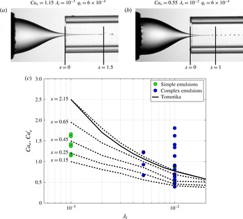
(a,b) The experimental shapes of simple jets for two values of the viscosity ratio. (c) The experimental values of the capillary numbers for which simple or compound drops are generated as a consequence of the capillary breakup of highly stretched steady capillary jets. In the case of simple emulsions,
 $Ca_{o}=\unicode[STIX]{x1D707}_{o}U/\unicode[STIX]{x1D70E}$
, and for double emulsions,
 $Ca_{o}^{\prime }=\unicode[STIX]{x1D707}_{o}U/(\unicode[STIX]{x1D70E}_{i}+\unicode[STIX]{x1D70E}_{m})$
. Observe that, in our experiments, the minimum values of the capillary numbers above which steady jets and, therefore, droplets with a low size dispersion are produced is well below the critical capillary number
 $Ca^{\ast }$
calculated under the parallel flow assumption (dispersion relation (4.4),
 $Ca^{\ast }\simeq 0.139\unicode[STIX]{x1D706}_{i}^{-1/2}$
). However, if the
 $x$
-dependent terms expressing the fact that the unperturbed jet diameter decreases downstream are included in the analysis (dispersion relation (5.1)), the agreement between observations and the predictions improves notably as
 $x$
lies within the realistic values depicted in panels (a) and (b). Dashed lines represent the values of the critical capillary number calculated using the dispersion relation (5.1) for fixed values of
 $x$
. All the results shown correspond to a value of the flow-rate ratio
 $q_{i}=10^{-3}$
. The values of the critical capillary number, however, are insensitive to variations of
 $q_{i}$
for
 $q_{i}\ll 1$
.

In figure 15 we have calculated
 $Ca^{\ast }(\unicode[STIX]{x1D706}_{i},q_{i})$
for fixed values of
 $x$
by finding the values of the critical capillary number in the dispersion relation (5.1) for given values of
 $\unicode[STIX]{x1D706}_{i}$
and
 $q_{i}$
, i.e. by solving the system
 $D^{\prime }(\unicode[STIX]{x1D714},k,x)=0$
and
 $\unicode[STIX]{x2202}D^{\prime }(\unicode[STIX]{x1D714},k,x)/\unicode[STIX]{x2202}k=0$
corresponding to
 $\text{Im}(\unicode[STIX]{x1D714})=0$
. The result, depicted in figure 15, shows that the effect of decreasing the value of
 $x$
in (5.1) and (5.2) (which is equivalent to increasing the value of
 $|{\dot{r}}_{j0}|$
and therefore increasing the thinning rate of the flow) is to decrease the value of the critical capillary number with respect to that predicted by the dispersion relation (4.4) corresponding to the case of purely cylindrical jets. Interestingly enough, the results obtained using the range of values of
 $x$
for which drops are emitted from the tip of the jets (see figure 15
a,b) are in good agreement with the experimental observations. Let us emphasize here that, as shown in Gordillo et al. (Reference Gordillo, Sevilla and Campo-Cortés2014), the higher stability exhibited by the types of stretched jets described here is not associated only with the term representing the stretching of the fluid elements,
 $2r_{j0}\dot{u}_{x}$
, which is well known to promote the stabilization of the flow (Eggers & Villermaux Reference Eggers and Villermaux2008).
Thanks to the strong stretching experienced by the simple or compound capillary jets generated using the confined selective withdrawal geometry presented in Evangelio et al. (Reference Evangelio, Campo-Cortés and Gordillo2015), the critical capillary number above which drops are regularly produced as a consequence of the capillary breakup of a steady jet is below the corresponding values characterizing other methodologies, like flow focusing (Gañán Calvo & Riesco-Chueca Reference Gañán Calvo and Riesco-Chueca2006; Gañán Calvo et al. Reference Gañán Calvo, Herrada and Garstecki2006, Reference Gañán Calvo, González, Riesco-Chueca and Herrada2007; Gañán Calvo Reference Gañán Calvo2008; Herrada et al. Reference Herrada, Montanero, Ferrera and Gañán Calvo2010). Therefore, thanks to the fact that the jets produced here are less slender than the jets created using other technologies, the confined selective withdrawal method possesses the advantage of producing simple or compound drops in a controllable way for comparatively small values of the outer capillary number, with the subsequent saving of energy and of outer liquid.
6 Conclusions
In this contribution, we have presented a practical method for the generation of simple or double emulsions, based on the capillary breakup of highly stretched capillary jets. These jets are produced when either one liquid or a couple of them are injected from either a nozzle or a coaxial nozzle within a co-flow of another liquid flowing from a pressurized reservoir towards a long extraction tube. The emulsions generated in such a way are composed of uniformly sized microdroplets if the Reynolds number characterizing the flow of the continuous phase,
 $Re_{o}$
, is of the order of unity or smaller and the capillary number is above a critical value
 $Ca^{\ast }$
of the order of unity. Under these conditions, our theoretical analysis provides analytical expressions for the drop generation frequencies,
 $f$
, and the diameters of the drops produced,
 $D_{d}$
. The equations for
 $f$
and
 $D_{d}$
are expressed as functions of the width of the extraction tube,
 $L$
, the mean velocity of the outer liquid in the extraction tube,
 $U$
, and the following dimensionless parameters: the viscosity ratio
 $\unicode[STIX]{x1D706}_{i}=\unicode[STIX]{x1D707}_{i}/\unicode[STIX]{x1D707}_{o}$
, with
 $\unicode[STIX]{x1D707}_{i}$
and
 $\unicode[STIX]{x1D707}_{o}$
the viscosities of the inner and outer fluids, respectively, the capillary number
 $Ca=\unicode[STIX]{x1D707}_{o}U/\unicode[STIX]{x1D70E}$
, with
 $\unicode[STIX]{x1D70E}$
the interfacial tension coefficient, and the flow-rate ratio
 $q_{i}=Q_{i}/(UL^{2})$
, with
 $Q_{i}$
the flow rate of the inner fluid. In the case of double emulsions, the parameter
 $\unicode[STIX]{x1D70E}=\unicode[STIX]{x1D70E}_{i}+\unicode[STIX]{x1D70E}_{m}$
in the definition of
 $Ca$
represents the addition of
 $\unicode[STIX]{x1D70E}_{i}$
, which is the interfacial tension coefficient between the inner and middle fluids, and
 $\unicode[STIX]{x1D70E}_{m}$
, which is the corresponding coefficient between the middle fluid and the continuous phase. The outer diameters of the drops composing the double emulsions are also dependent on the parameter
 $q=Q/(UL^{2})$
, with
 $Q$
the sum of the flow rates of the inner and middle fluids. The equations provided for
 $f$
and
 $D_{d}$
are valid whenever
 $Ca>Ca^{\ast }(\unicode[STIX]{x1D706}_{i},q_{i})$
, with
 $Ca^{\ast }\simeq Ca^{\ast }(\unicode[STIX]{x1D706}_{i})$
in the limit
 $q_{i}\ll 1$
. This fact indicates that uniformly sized droplets with arbitrary small diameters can be produced using this methodology. This is so because, under these circumstances, the analysis predicts that the simple or compound capillary jets are globally stable, namely, steady, at the entrance of the extraction tube and, in addition, our results indicate that the drop formation frequencies are those for which the capillary instabilities in the cylindrical portion of the jet grow faster. The values of
 $Ca^{\ast }$
above which a steady jet is formed, namely, the flow is globally stable, are well predicted by a local spatio-temporal stability analysis, but only when the leading-order terms expressing that the unperturbed solution varies downstream are included in the analysis. In agreement with the experimental observations, our theory reveals that the highly stretched capillary jets generated using the present design are more stable than the slightly convergent cylindrical jets generated using other methodologies. This is the reason behind the fact that the critical capillary numbers above which stable jets are produced in the confined selective withdrawal geometry are smaller than in the flow focusing one, a geometry for which it has been reported that the dependence of the critical capillary number on the viscosity ratio is of the form
 $Ca^{\ast }=0.139\unicode[STIX]{x1D706}_{i}^{-1/2}$
(Gañán Calvo & Riesco-Chueca Reference Gañán Calvo and Riesco-Chueca2006; Gañán Calvo et al.
Reference Gañán Calvo, Herrada and Garstecki2006, Reference Gañán Calvo, González, Riesco-Chueca and Herrada2007; Gañán Calvo Reference Gañán Calvo2008).
Moreover, since the analytical description of capillary jets surrounded by another liquid is still far from being comparable to the advances accomplished in the analysis of the analogous case of liquid jets in air, we have also provided a theoretical framework, based on a slender-body approach, to describe the steady shapes of axisymmetric simple or compound jets flowing within an immiscible liquid in the limits
 $Re_{o}\gg 1$
and
 $Re_{o}\lesssim O(1)$
. Our theory is in excellent agreement with experimental observations.
Acknowledgements
This work has been supported by the Spanish MINECO under Project DPI2014-59292-C3-2-P, partly financed through European funds. The authors are grateful to Professor Ignacio González Loscertales for providing us with a coaxial injection tube.
Appendix A. Local stability analysis of steady jets at low Reynolds number
The dispersion relation to be deduced in what follows is built up starting from the unsteady continuity equation
 $$\begin{eqnarray}\displaystyle \frac{\unicode[STIX]{x2202}r_{j}^{2}}{\unicode[STIX]{x2202}t}+\frac{\unicode[STIX]{x2202}}{\unicode[STIX]{x2202}x}\left[(u_{x}+fr_{j}^{2})r_{j}^{2}-\frac{r_{j}^{4}}{8\unicode[STIX]{x1D706}_{i}}\frac{\unicode[STIX]{x2202}p_{i}}{\unicode[STIX]{x2202}x}\right]=0, & & \displaystyle\end{eqnarray}$$
which needs to be solved together with the kinematic condition at the jet interface, which differs from (3.11) in that, in this case, unsteady terms need to be retained:
 $$\begin{eqnarray}\displaystyle u_{r}^{\prime }=\frac{\unicode[STIX]{x2202}r_{j}}{\unicode[STIX]{x2202}t}+[u_{x}(x)+f(x)r_{j}^{2}]\frac{\text{d}r_{j}(x)}{\text{d}x}+\frac{r_{j}}{2}\frac{\text{d}u_{x}(x)}{\text{d}x}+\frac{r_{j}^{3}}{4}\frac{\text{d}f}{\text{d}x}(x). & & \displaystyle\end{eqnarray}$$
In (A 1) and (A 2), the dimensionless time is related to its dimensional counterpart as
 $t=TU/L$
.
Since the local stability analysis will be performed in a portion of the jet that is far from the nozzle, where the flow is slender, i.e. where
 $\text{d}r_{j0}/\text{d}x\ll 1$
, the perturbed radial velocity field created by the presence of the jet is approximated here, following the explanation given after (3.9), as
 $$\begin{eqnarray}\displaystyle u_{r}^{\prime }\simeq \frac{s(x,t)}{r}\quad \Rightarrow \quad \frac{\unicode[STIX]{x2202}u_{r}^{\prime }}{\unicode[STIX]{x2202}r}(r=r_{j})=-\frac{u_{r}^{\prime }}{r_{j}}. & & \displaystyle\end{eqnarray}$$
Introducing (A 2) and (A 3) into (3.17) and substituting the resulting expression into the unsteady mass conservation equation (A 1) yields the following dimensionless partial differential equation for
 $r_{j}(x,t)$
:
 $$\begin{eqnarray}\displaystyle & & \displaystyle \frac{\unicode[STIX]{x2202}r_{j}}{\unicode[STIX]{x2202}t}\left[2r_{j}+\frac{1}{4\unicode[STIX]{x1D706}_{i}}\left(2r_{j}\left(\frac{\unicode[STIX]{x2202}r_{j}}{\unicode[STIX]{x2202}x}\right)^{2}+r_{j}^{2}\frac{\unicode[STIX]{x2202}^{2}r_{j}}{\unicode[STIX]{x2202}x^{2}}\right)\right]-\frac{1}{2\unicode[STIX]{x1D706}_{i}}r_{j}^{2}\frac{\unicode[STIX]{x2202}r_{j}}{\unicode[STIX]{x2202}x}\frac{\unicode[STIX]{x2202}}{\unicode[STIX]{x2202}x}\left(\frac{\unicode[STIX]{x2202}r_{j}}{\unicode[STIX]{x2202}t}\right)-\frac{1}{4\unicode[STIX]{x1D706}_{i}}r_{j}^{3}\frac{\unicode[STIX]{x2202}^{2}}{\unicode[STIX]{x2202}x^{2}}\left(\frac{\unicode[STIX]{x2202}r_{j}}{\unicode[STIX]{x2202}t}\right)\nonumber\\ \displaystyle & & \displaystyle \quad +\,\frac{\unicode[STIX]{x2202}}{\unicode[STIX]{x2202}x}\left[(u_{x}+fr_{j}^{2})r_{j}^{2}+\frac{1}{8\unicode[STIX]{x1D706}_{i}}\left(-3r_{j}^{4}\frac{\text{d}^{2}u_{x}}{\text{d}x^{2}}-3r_{j}^{6}\frac{\text{d}^{2}f}{\text{d}x^{2}}-4fr_{j}^{4}-Ca^{-1}r_{j}^{4}\frac{\unicode[STIX]{x2202}\unicode[STIX]{x1D712}}{\unicode[STIX]{x2202}x}-6r_{j}^{5}\frac{\unicode[STIX]{x2202}r_{j}}{\unicode[STIX]{x2202}x}\frac{\text{d}f}{\text{d}x}\right.\right.\nonumber\\ \displaystyle & & \displaystyle \quad \left.\left.-\,2\left(\frac{\unicode[STIX]{x2202}r_{j}}{\unicode[STIX]{x2202}x}\right)^{2}fr_{j}^{4}+2r_{j}^{2}\left(\frac{\unicode[STIX]{x2202}r_{j}}{\unicode[STIX]{x2202}x}\right)^{2}u_{x}-2r_{j}^{3}\frac{\unicode[STIX]{x2202}r_{j}}{\unicode[STIX]{x2202}x}\frac{\text{d}u_{x}}{\text{d}x}-2u_{x}r_{j}^{3}\frac{\unicode[STIX]{x2202}^{2}r_{j}}{\unicode[STIX]{x2202}x^{2}}-2fr_{j}^{5}\frac{\unicode[STIX]{x2202}^{2}r_{j}}{\unicode[STIX]{x2202}x^{2}}\right)\right]=0.\nonumber\\ \displaystyle & & \displaystyle\end{eqnarray}$$
Assuming that the wavelength of the perturbation is much smaller than the length along which the steady jet radius experiences variations of its same order of magnitude, with this condition clearly verified for
 $x\gtrsim O(1)$
, we look for travelling-wave solutions to (A 4) of the form
 $$\begin{eqnarray}\displaystyle r_{j}=r_{j0}(x)+\text{e}^{\text{i}(\bar{k}x-\bar{\unicode[STIX]{x1D714}}t)}r_{j1}, & & \displaystyle\end{eqnarray}$$
with
 $r_{j0}$
the unperturbed jet radius. In (A 5),
 $\bar{k}=KL$
and
 $\bar{\unicode[STIX]{x1D714}}=\unicode[STIX]{x1D6FA}L/U$
indicate, respectively, the dimensionless counterparts of the dimensional wavenumber
 $K$
and the dimensional frequency
 $\unicode[STIX]{x1D6FA}$
. Once the ansatz (A 5) is introduced into (A 4), and retaining only linear terms in
 $r_{j1}$
in the resulting expression, this yields
 $$\begin{eqnarray}\displaystyle D^{\prime }(\unicode[STIX]{x1D714},k,x) & = & \displaystyle -\text{i}\unicode[STIX]{x1D714}\left(2+\frac{k^{2}}{4\unicode[STIX]{x1D706}_{i}}-\text{i}k\frac{{\dot{r}}_{j0}}{2\unicode[STIX]{x1D706}_{i}}\right)+\text{i}k\left[2u_{x}+fr_{j0}^{2}\left(4-\frac{2}{\unicode[STIX]{x1D706}_{i}}\right)+\frac{{\dot{r}}_{j0}}{2Ca\unicode[STIX]{x1D706}_{i}}\right]\nonumber\\ \displaystyle & & \displaystyle -\,k^{2}\left[\frac{1}{8\unicode[STIX]{x1D706}_{i}Ca}-\frac{r_{j0}\dot{u}_{x}}{2\unicode[STIX]{x1D706}_{i}}-\frac{r_{j0}^{3}\,{\dot{f}}}{\unicode[STIX]{x1D706}_{i}}-{\dot{r}}_{j0}\left(\frac{7}{4\unicode[STIX]{x1D706}_{i}}r_{j0}^{2}\,f+\frac{u_{x}}{4\unicode[STIX]{x1D706}_{i}}\right)\right]\nonumber\\ \displaystyle & & \displaystyle +\,\text{i}k^{3}\left(\frac{u_{x}}{4\unicode[STIX]{x1D706}_{i}}+\frac{fr_{j0}^{2}}{4\unicode[STIX]{x1D706}_{i}}-\frac{5{\dot{r}}_{j0}}{8Ca\unicode[STIX]{x1D706}_{i}}\right)+\frac{k^{4}}{8\unicode[STIX]{x1D706}_{i}Ca}+\unicode[STIX]{x1D6FD}(x)=0,\end{eqnarray}$$
with
 $$\begin{eqnarray}\displaystyle \unicode[STIX]{x1D6FD}(x)=2\frac{\text{d}}{\text{d}x}(u_{x}r_{j0})+\frac{{\dot{r}}_{j0}^{2}+\ddot{r}_{j0}r_{j0}}{4\unicode[STIX]{x1D706}_{i}Ca}+4r_{j0}^{3}\,{\dot{f}}-\frac{2r_{j0}^{3}\,{\dot{f}}}{\unicode[STIX]{x1D706}_{i}}+fr_{j0}^{2}{\dot{r}}_{j0}\left(12-\frac{6}{\unicode[STIX]{x1D706}_{i}}\right). & & \displaystyle\end{eqnarray}$$
In (A 6) the local dimensionless variables
 $\unicode[STIX]{x1D714}(x)=\bar{\unicode[STIX]{x1D714}}r_{j0}(x)\sim O(1)$
and
 $k=\bar{k}r_{j0}(x)\sim O(1)$
have been defined. To deduce the dispersion relation (A 6), we have retained only order-unity terms as well as the leading-order non-parallel terms, i.e. those with an order of magnitude
 ${\sim}O({\dot{r}}_{j0}(x))\ll 1$
. The interested reader is directed to the appendix of Gordillo et al. (Reference Gordillo, Sevilla and Campo-Cortés2014) for further algebraic details.