

1. Introduction
The vortex-induced vibration (VIV) response of various systems have been investigated in early studies by modelling the system as a flexibly mounted rigid cylinder placed in a flow, free to oscillate with one degree-of-freedom (DOF) in the transverse (crossflow) direction (Bearman Reference Bearman1984; Khalak & Williamson Reference Khalak and Williamson1999; Govardhan & Williamson Reference Govardhan and Williamson2002; Sarpkaya Reference Sarpkaya2004; Raghavan & Bernitsas Reference Raghavan and Bernitsas2011). The complex dynamic response of the structures coupled with their surrounding flow has been investigated to characterize the fundamentals of the fluid–structure interaction response for such systems. In many real world applications, such as mooring lines used to stabilize the offshore oil platforms and the conceptual designs for offshore wind turbines, VIV is observed in long flexible cylinders, where oscillations are possible in both the crossflow and streamwise (inline) directions. Later studies have investigated the influence of the second DOF in the inline direction on the overall VIV response of a circular cylinder (Sarpkaya Reference Sarpkaya1995; Jauvtis & Williamson Reference Jauvtis and Williamson2004; Dahl, Hover & Triantafyllou Reference Dahl, Hover and Triantafyllou2006; Dahl et al. Reference Dahl, Hover, Triantafyllou, Dong and Karniadakis2007). These studies have demonstrated that giving the structure a second DOF in the inline direction can change the dynamic response of the system, significantly. In an experimental study on a two DOF VIV response of a circular cylinder (Dahl et al. Reference Dahl, Hover, Triantafyllou, Dong and Karniadakis2007), the ratio between the crossflow to inline natural frequency of the system was altered systematically to study the impact of the system's frequency ratios on the overall VIV response of the system. It was concluded that under perfect vortex shedding resonance, in which the inline natural frequency of the system is twice the crossflow natural frequency, a fundamental change in both the orbital motion of the structure and the frequency content of the fluid forces occurs. The VIV response of the system was observed to be dominated by a complex vortex wake, resulting in high frequency lift forces. In VIV applications such large contributions of higher harmonics of the lift force could consequently contribute to the fatigue life of structures undergoing large amplitude VIV. Additionally, flow-induced vibration of a circular cylinder, placed in the wake of a stationary upstream cylinder, with two DOF in both the inline and crossflow directions has been studied (Chaplin & Batten Reference Chaplin and Batten2014). The results suggested that the presence of both the inline and crossflow DOF, and additionally the presence of higher modes can significantly influence some features of the fluid–structure interactions when compared with those of an isolated cylinder with one DOF.
While VIV studies of elastically mounted rigid cylinders have facilitated our understanding of VIV occurring in a more complex case of flexible cylinders, the VIV response of a flexible cylinder can undergo complex large amplitude oscillations at higher vibrational modes, due to the additional variables associated with dynamics of flexible systems. Experimental (Chaplin et al. Reference Chaplin, Bearman, Huarte and Pattenden2005; Trim et al. Reference Trim, Braaten, Lie and Tognarelli2005; Vandiver et al. Reference Vandiver, Marcollo, Swithenbank and Jhingran2005; Lie & Kaasen Reference Lie and Kaasen2006; Huera-Huarte & Bearman Reference Huera-Huarte and Bearman2009; Seyed-Aghazadeh & Modarres-Sadeghi Reference Seyed-Aghazadeh and Modarres-Sadeghi2016; Seyed-Aghazadeh, Edraki & Modarres-Sadeghi Reference Seyed-Aghazadeh, Edraki and Modarres-Sadeghi2019), and numerical (Evangelinos, Lucor & Karniadakis Reference Evangelinos, Lucor and Karniadakis2000; Bourguet, Karniadakis & Triantafyllou Reference Bourguet, Karniadakis and Triantafyllou2011a; Bourguet et al. Reference Bourguet, Modarres-Sadeghi, Karniadakis and Triantafyllou2011b; Bourguet, Karniadakis & Triantafyllou Reference Bourguet, Karniadakis and Triantafyllou2013; Zanganeh & Srinil Reference Zanganeh and Srinil2016) studies have well documented the VIV response of a flexible cylinder, placed perpendicular to the flow. Excitation of mono- and multi-frequency modes and transition from lower modes to higher modes excitation have been observed in the VIV response of such flexible cylinders. In addition, a travelling wave observed in the VIV response of flexible cylinders (Marcollo et al. Reference Marcollo, Eassom, Fontaine, Tognarelli, Beynet, Constantinides and Oakley2011; Bourguet, Lucor & Triantafyllou Reference Bourguet, Lucor and Triantafyllou2012; Seyed-Aghazadeh et al. Reference Seyed-Aghazadeh, Benner, Gjokollari and Modarres-Sadeghi2021) adds to the complexity of the response that cannot be characterized in simpler models of a flexible cylinder, i.e. flexibly mounted cylinder studies with one or two DOF.
Most VIV studies on flexible cylinders have considered the flexible cylinder to be a tension-dominated one. If the flexible tension-dominated cylinder can be modelled as a string under oscillations in fluid flow, the ratio between the system's natural frequencies in both the crossflow and inline directions is approximately multiple integers, i.e. the second natural frequency will have values twice the fundamental frequency, the third natural frequency will be thrice the fundamental frequency and so on. In a recent study, the VIV response of a bending-dominated cylinder has been studied experimentally (Gedikli, Chelidze & Dahl Reference Gedikli, Chelidze and Dahl2018), in which the ratio between the system's natural frequencies was designed to take different values in each directions. It was concluded that independent from the natural frequency ratios in the crossflow and inline directions, the inline response is a forced response that depends heavily on the crossflow response of the system. The VIV response of the cylinder in the inline direction was found to be unlikely to oscillate with an even mode shape due to symmetric drag loading, even when the system was tuned to have an even mode to be excited at the expected frequency of vortex shedding. This observation has been different from those reported for a tension-dominated flexible cylinder for which both odd and even modes have been excited in the crossflow and inline directions (Seyed-Aghazadeh & Modarres-Sadeghi Reference Seyed-Aghazadeh and Modarres-Sadeghi2016; Seyed-Aghazadeh et al. Reference Seyed-Aghazadeh, Edraki and Modarres-Sadeghi2019).
The question that arises here is what if the flexible cylinder cannot be modelled as either a tension-dominated or bending-dominated one and the frequency ratios in each direction have non-integer values as one would expect to see for a beam under tension? How the VIV response of the system will be compared with those of a tension-dominated or bending-dominated one? Our understanding of the complex multi-modal VIV behaviour in such flexible cylinders can be well improved if a study can be designed to accommodate for a systematic and controlled change in the system's natural frequencies and structural excitation at a single or multiple modes higher than one, while some complex features of the response, such as travelling wave behaviour, can be limited or entirely eliminated. This is the goal in our current study.
Recent experimental studies have investigated the VIV in a dual mass system, where the oscillating cylinder subjected to the incoming flow has two DOF to oscillate in the crossflow direction (Nishi Reference Nishi2013; Nishi, Fukuda & Shinohara Reference Nishi, Fukuda and Shinohara2017). These studies have investigated the advantages of using such a dual mass system in expanding the flow velocity range at which large amplitude oscillations could occur. These studies have shown the selective advantages of such systems in energy harvesting over a wider excitation range in the VIV response of the system; the excitation was first observed for the flow velocity range at which the oscillation frequency locked into the first eigenfrequency of the system, and later shifted to a limited range of velocities over which lock-in occurred at frequencies close to the second eigenfrequency of the system. However, the experimental apparatus design in these studies limited the upper ranges of flow velocities at which the system could be tested and, therefore, the results were limited to VIV oscillations observed up to only the onset of excitation at the second eigenfrequencies. Similarly, in a recent theoretical study (Vicente-Ludlam, Barrero-Gil & Velazquez Reference Vicente-Ludlam, Barrero-Gil and Velazquez2015), the galloping response of a dual mass system has been studied using the quasi-steady assumption. Improvements in the energy extraction efficiencies have been studied by tuning the mechanical system properties of the system.
While the recent studies on the VIV of a dual mass system, free to oscillate with two DOF in the crossflow direction, have shed light on their potentials to be used in fluidic energy harvester designs to extend their operating range, there is still a gap in our understanding of the fundamentals of VIV in multiple DOF systems, in particular when (a) there is no limitation in the experimental set-up to prevent the VIV response to cover excitation at both the first and second eigenfrequencies of the system, and (b) the eigenfrequency ratios can be systematically varied to study a wide range of VIV response occurrences, from mono-frequency excitation at each eigenfrequency to a multi-modal excitation over overlapping flow velocities, over which interaction between the excited modes can be studied. These goals will be achieved in our current study where VIV of a two DOF elastically mounted rigid cylinder, free to oscillate in the crossflow direction at its first two eigenfrequencies, is studied experimentally. We have developed a unique experimental set-up that would realize the study of the VIV response of a two DOF elastically mounted circular cylinder at both its eigenmodes. The two eigenfrequencies of the system include one at the lower first mode and one at the higher second mode. The cylinder in our study was mounted on an air-bearing set-up, allowing frictionless motion of the cylinder in the crossflow direction, and placed vertically in the test section of a recirculating water tunnel. The unique air-bearing set-up design allows for testing a variation of eigenfrequency ratios of the system, which in return can facilitate understanding of the physical mechanisms responsible for the VIV of multi-DOF cylinders when excited at higher vibrational modes. The dynamic response of the cylinder is studied for a range of flow velocities in the range of  $U=0.04\unicode{x2013}0.31\,{\rm m}\,{\rm s}^{-1}$, corresponding to a Reynolds number range of
 $Re=1033\unicode{x2013}7478$.
In what follows, § 2 describes the experimental set-up and methodology used to capture the VIV response of the system. Section 3 presents theoretical modal analysis of the forced vibration of a system with two DOF and describes the system's eigenfrequencies and eigenmodes. The results presented in § 4 describe the overall VIV response of the system over the entire range of reduced velocities tested for a range of eigenfrequency ratios of the system. Section 4.1 describes the amplitudes and frequencies of oscillations as well as response phase evolution over a wide range of flow velocities and eigenfrequency ratios. Section 4.2 presents the flow forces acting on the cylinder. Section 4.3 presents the qualitative and quantitative wake structure at a sample eigenfrequency ratio for the entire range of flow velocities previously tested. A full map of vortex shedding patterns is presented at a sample eigenfrequency ratio of the system. Finally, § 4.4 presents the prevalent shedding modes in the wake of the cylinder undergoing VIV using the technique of proper orthogonal decomposition (POD).
2. Experimental set-up and data collection
2.1. Structural response measurements
The experiments were conducted in a recirculating water tunnel, with a test section of  $0.45\, {\rm m} \times 0.45\, {\rm m} \times 1.5\, {\rm m}$ and a turbulence intensity of less than 1 % for up to a velocity of
 $1\ {\rm m}\,{\rm s}^{-1}$. A uniform circular cylinder with a diameter of
 $D = 21.6\,{\rm mm}$, immersed length of
 $L= 250\,{\rm mm}$ and an aspect ratio of
 $L/D=11.57$ was tested. The mass ratio of the cylinder was calculated to be
 $m^{*}=4 m / {\rm \pi}\rho D^{2} L=21.1$, where
 $m$ is total moving mass of the system and
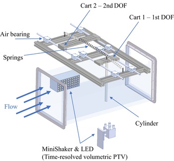
 $\rho$ is the flow density. The cylinder was attached to an air-bearing set-up, allowed to oscillate in the transverse (crossflow) direction. A schematic of the set-up is shown in figure 1. The air-bearing set-up had eight air bearings, each pair mounted on ceramic coated aluminium shafts running in parallel, to reduce the structural damping in the system. Two moving carts were mounted on aluminium shafts, each free to oscillate smoothly, constraining the motion to two DOF in the crossflow direction only. The elasticity in the system was provided by two identical springs with stiffness
 $k_1$ that were attached from the moving carts to a fixed housing, together with a central spring with stiffness
 $k_2$ that connected the two moving carts together. The cylinder was attached to one of the carts (cart 1) and placed in the test section of the water tunnel, being subjected to fluid flow. The motion of cart 1 holding the cylinder in the flow was transmitted to cart 2 through the central spring (
 $k_2$).
Schematic of the experimental apparatus.

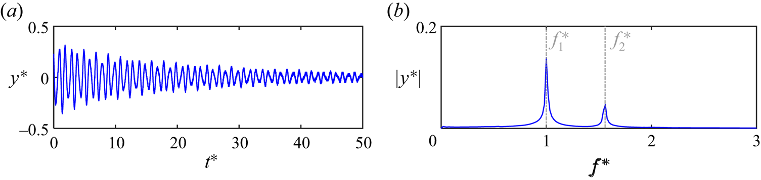
Two laser displacement sensors (Panasonic HL-G1 series) were synchronously used to record displacement data of the oscillating carts in the crossflow direction. The oscillations of the carts were recorded for 120 s, sampled at a rate of 500 Hz, capturing at least 50 cycles of oscillations of the cylinder. Decay tests were conducted in still water and air to obtain the two natural frequencies and damping ratios of the system at each mode by giving the system an initial displacement and releasing it to oscillate freely while recording the amplitude of oscillations. Figure 2(a) shows a sample decay test response in still water in terms of time series of amplitude of oscillations normalized by the diameter of the cylinder,  $y^*$. The first natural frequency of the system is used to make the time dimensionless,
 $t^*$. Figure 2(b) shows the frequency content of the free decay response analysed through fast Fourier transform (FFT). This air-bearing set-up enabled us to change the ratio between the first two natural frequencies by replacing the central spring in the set-up and varying its stiffness, while keeping the side springs untouched. This would yield to a constant first natural frequency of the system, while changing the second natural frequency of the system. The first natural frequency of the system in still water was measured to be
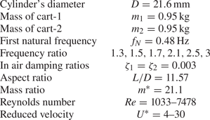
 $f_{N_1}= 0.48$ Hz, following the free decay tests. Table 1 summarizes the first and second natural frequencies and damping ratios of the system, obtained from the free decay tests. The natural frequencies for first and second modes were used to calculate first and second reduced velocities, respectively, as
 $U^*_i={U}/{f_{N_iD}}$ for
 $i=1$ and 2, where
 $U$ is the flow velocity, and
 $f_N$ is the natural frequency of the system at each mode.
Free decay response sample for the eigenfrequency ratio of  $R=1.5$. (a) Time history of normalized amplitude of oscillations (
 $y^*$) versus normalized time (
 $t^*$), and (b) normalized frequency content of the response. The in-water damping ratio is obtained as 0.008 from free decay tests.

Experimental parameters and the test cylinder's structural characteristics.

A six-axis force sensor (ATI-Nano17 IP65) was used to measure the total flow forces of the cylinder in the crossflow and inline directions. The displacement data measured through the laser displacement sensors was synchronised with the measured flow forces obtained through the force sensor. During these experiments, the water level was held constant and the flow velocity was increased from zero in small steps of  $0.003\ {\rm m}\,{\rm s}^{-1}$. The system's response in the crossflow direction was measured for the Reynolds number range of
 $Re=1033\unicode{x2013}7478$, corresponding to a reduced velocity range of
 $U^*=4\unicode{x2013}30$, calculated based on the system's first natural frequency. Details of the test matrix and governing dimensionless system parameters are given in table 1.
2.2. Qualitative and quantitative flow visualization
Both qualitative and quantitative flow visualization tests were conducted to study vortex dynamics in the wake of the cylinder. For qualitative flow visualization purposes, the hydrogen bubble visualization technique was used. The hydrogen bubble generation technique works based on the electrolysis of water. A platinum wire with a diameter of 0.0508 mm was strung across the test section perpendicular to the flow and the spanwise length of the cylinder. The platinum wire served as a cathode, while a 50–100 V, 2 A power supply positively charged a graphite plate to serve as an anode. The potential between the two caused a build-up of hydrogen bubbles on the platinum wire. The bubbles separated from the wire once their diameter exceeded the wire diameter, creating a bubble film that was used to view the vortex structures in the wake of the cylinder. A high-speed camera (Victorem 32B216MCX), placed underneath the water tunnel's test section, was employed to record the instantaneous wake structure from the bottom view capturing images at 200 frames per second at a spanwise location of  $z=0.5$ along the length of the cylinder measured from the water free surface, where
 $z$ is the dimensionless spanwise location normalized by the length of the cylinder. To illuminate the bubble sheet, light-emitting diode (LED) lightings were mounted on each side of the test section at an angle to ensure uniform lighting conditions.
For quantitative flow measurement purposes, a time-resolved volumetric particle tracking velocimetry (PTV) technique was used to measure the flow field dynamics in the wake of the cylinder at sample reduced velocities. The flow field dynamics were measured in a time-resolved fashion using the state-of-the-art three-dimensional (3-D) Lagrangian PTV system (Shake-the-Box, LaVision Inc., Ypsilanti, MI, USA). The shake-the-box system uses a ‘MiniShaker’ integrated camera system and a flashlight LED array for recording and illumination of the seeding particles, respectively. Seeding particles used were polyamide high-quality hollow glass spheres of  $60\,\mathrm {\mu }{\rm m}$ nominal diameter. The particle concentration used was approximately
 $0.02\,{\rm g}\,{\rm l}^{-1}$. Particles were illuminated by a
 $300 \times 100\,{\rm mm}^2$ LED (FLASHLIGHT
 $300$ array, LaVision Inc.) with 72 high-power LEDs that were operated above the nominal LED current to generate short pulses at very high light intensities. The recording system including the four pre-aligned digital cameras in the MiniShaker box were equipped with 16 mm lenses to capture images at
 $120$ Hz trigger rate at full resolution (
 $1984\times 1264$). Multiple separate subsets of 1200 images corresponding to
 $20$ s of measurement (which cover the minimum of eight cycles of the cylinder's oscillation) were acquired at each sample reduced velocity. The flashlight and set of cameras were triggered simultaneously using a LaVision programmable timing unit driven by DaVis 10 acquisition software. Cameras were calibrated using a 3-D calibration plate with two planes with calibration marks separated by the pre-defined distance between its two planes. A polynomial fit that uses a third-order polynomial was integrated to model the perspective and optical image distortion for the mapping from a world plane to the CCD camera sensor. The shake-the-box algorithm that uses the 3-D Lagrangian PTV method allowed for measurements of densely seeded flows at the highest spatial resolution. The particle-based tracking method built into this method uses an iterative particle reconstruction technique combined with an advanced four-dimensional PTV algorithm using the time information for the reconstruction process of particle trajectories. In the shake-the-box algorithm, the available velocity information is used to estimate particle distribution compared with previous methods in which first the particle distribution is determined followed by a deduction of the velocity (Schanz, Gesemann & Schröder Reference Schanz, Gesemann and Schröder2016). This algorithm can achieve a higher reconstruction accuracy at much faster processing speed compared with the tomographic particle imaging velocimetry (Chen, Wu & Cheng Reference Chen, Wu and Cheng2019).
Figure 1 shows the schematic of the PTV measurement set-up, and locations of the LED flashlight and MiniShaker camera box used in this system. The platinum wire used in the hydrogen bubble generation process was placed horizontally in the test section of the water tunnel located at a distance of one cylinder diameter upstream of the cylinder (not shown in the schematics).
3. Theoretical modal analysis
The experimental set-up shown in figure 1 can be modelled as a two DOF system. The equations of motion of this two DOF system can be written as
 \begin{gather} m_1{\ddot{y}}_1+\left(c_1+c_{2}\right){\dot{y}}_1-c_2{\dot{y}}_2+\left(k_1+k_{2}\right)y_1-k_2y_2=F_y(t), \end{gather}
 \begin{gather} m_2{\ddot{y}}_2+\left(c_{1}+c_2\right){\dot{y}}_2-c_2{\dot{y}}_1+\left(k_{1}+k_2\right)y_2-k_2y_1=0, \end{gather}
where  $m_i$,
 $k_i$ and
 $c_i$ denote the mass, stiffness and damping of the system, respectively. The displacement in the crossflow direction with respect to the zero equilibrium position of the system is denoted by
 ${y}_i$. The subscript
 $i=1,2$ stands for the crossflow DOF for cart 1 and cart 2, respectively. The dot symbol indicates the derivative with respect to time. Here
 $F_y(t)$ is the instantaneous fluid force on the submerged cylinder, connected to cart 1, which can be used to calculate the crossflow force coefficient,
 $C_y(t)= 2 F_y(t)/\rho D U^2 L$;
 $\rho$ is the fluid density,
 $U$ is the flow velocity and
 $D$ is the diameter of the cylinder. The numerical values of the parameters used for the two DOF system are provided in table 1. The system has two fundamental eigenfrequencies of
 $f_1$ and
 $f_2$ with the corresponding mode shapes of
 ${\boldsymbol{\mathsf{\Phi}}} _1=[1,1]^{{\rm T}}$ and
 ${\boldsymbol{\mathsf{\Phi}}} _2=[1,-1]^{{\rm T}}$, respectively. For a harmonic excitation of
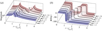
 $F_y(t)=F_0 {\rm e}^{{\rm i}(2{\rm \pi} f_{ext}) t}$, figure 3(a) shows the magnitude of frequency-response function (FRF) curves of cart 1 for the different values of
 $k_2$. The plot shows that the first eigenfrequency of the system remains constant, independent from changes in the value of
 $k_2$, whereas the second eigenfrequency increases with any increase in the value of
 $k_2$, resulting in eigenfrequency ratios (
 $R=f_2/f_1$) between 1.3 and 3.0 for the system. Figure 3(b) shows the phase of FRF curves of cart 1 for the different values of
 $k_2$. It shows that the displacement remains in phase with forcing for frequencies smaller than the first eigenfrequency of the system, and experiences a sudden transition to out-of-phase at the frequencies very close to the resonance (
 $r=1$). This is a typical behaviour observed in systems with a very low damping ratio (
 $\zeta \ll 1$). The experimental set-up in our current study is designed to uniquely achieve such a low damping ratio. A similar behaviour is observable in frequency regions near the second eigenfrequency of the system.
Frequency-response function curves of the two DOF system for different frequency ratios.

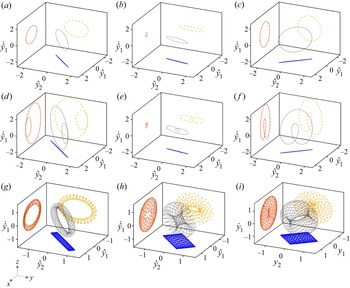
The two DOF system's response to fluid forces in the crossflow direction,  $F_y(t)$, can include single or multiple harmonics. These harmonics may or may not match the eigenfrequencies of the system in general. The FFT plot can be used to analyse the frequency content of the oscillation, but a FFT plot does not provide any information on which mode shapes of the system are excited. In a nonlinear system, for example, a FFT plot with multiple frequency peaks can be either associated with a multi-modal oscillation or a multi-harmonic oscillation. In a multi-modal oscillation, multiple modes of the system are excited at their corresponding eigenfrequencies, whereas in a multi-harmonic oscillation only one mode is excited at multiple different frequencies. To distinguish between these two different dynamic responses, periodic orbits in the 3-D space of
 $(y_1,y_2,\dot {y}_1)$, shown in figure 4, can be used to visually differentiate between a single harmonic oscillation, a multi-modal oscillation and a multi-harmonic oscillation for a two DOF system. The projection in the
 $x$–
 $y$ plane provides information on mode shapes that have been excited, whereas the projection in the
 $x$–
 $z$ or
 $y$–
 $z$ planes provides information on frequency contents of the oscillation. The periodic orbits are commonly used in nonlinear dynamic studies to visualize the steady-state response of a nonlinear system (Ardeh & Allen Reference Ardeh and Allen2013).
Periodic orbits of a two DOF system at (a–c) single harmonic motions, (d–f) higher harmonic motions and (g–i) multi-modal motions.

The first row plots in figure 4(a–c) show samples for the periodic orbits of a two DOF system for a single harmonic oscillation, where the excitation frequencies are selected as  $f_{ext}=f_1,(f_1+f_2)/2$ and
 $f_2$, respectively. Here
 $y_1$ and
 $y_2$ are normalized displacements with respect to the maximum oscillation amplitude,
 $y_{max}$, obtained for
 $y_1$ and
 $y_2$ in our simulations;
 $\dot {y}_1$ is normalized with respect to
 $2{\rm \pi} f_1y_{max}$. The hat symbol in these figures denotes the normalized values. The sample eigenfrequency ratio is set to
 $R= 1.7$. In the first row plots, the projection of periodic orbits in the
 $x$–
 $y$ plane forms an ellipse (approximately a line here due to very small damping ratios) with
 ${+}45^{\circ }$ and
 ${-}45^{\circ }$ orientations for
 $f_{ext}=f_1$ and
 $f_2$, representing harmonic oscillation around the
 $1$st mode shape and the
 $2$nd mode shape of the system, respectively. The projection takes a form between the projection for the
 $1$st mode shape and
 $2$nd mode shape if the system is excited at a frequency that does not match the fundamental eigenfrequencies of the system, similar to the one shown in figure 4(b). The second and third row plots in figure 4(d–i) show the difference between periodic orbits of a multi-harmonic oscillation and a multi-modal oscillation for the two DOF system, respectively. In a multiharmonic oscillation (second row), the projection of periodic orbits in the
 $x$–
 $y$ plane shows that only the
 $1$st mode or
 $2$nd mode, or a linear combination of them are excited, even though the projection in the
 $x$–
 $z$ or
 $y$–
 $z$ planes shows existence of two harmonics (two closed circles). The third row plots in figure 4(g–i) show the case of a multi-modal oscillation where the
 $1$st and
 $2$nd mode shapes of the system are excited by a harmonic excitation such as
 $F_y(t)=F_1 {\rm e}^{({\rm i}(2{\rm \pi} f_1) t)}+F_2 {\rm e}^{({\rm i}(2{\rm \pi} f_2) t)}$, where
 $F_2=F_1$,
 $F_2=4F_1$ and
 $F_2=8 F_1$, respectively. The projection of periodic orbits in the
 $x$–
 $y$ plane shows a transition from the
 $1$st mode being dominantly excited to the
 $2$nd mode being dominantly excited. To study the modal transition in our experimental VIV study, we have obtained similar plots for our experiments that will be discussed in our results. Such an analysis provides us with a powerful tool to better characterize the dynamic VIV response of the system and distinguish between a multi-modal oscillation or a multi-harmonic oscillation in the system.
4. Results
4.1. Structural response of the system
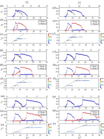
In this section an overall view of the VIV response is given for the experimental campaign discussed in the present work, where the cylinder is allowed to oscillate with two DOF in the crossflow direction only. The response is discussed for a range of eigenfrequency ratios of  $R=1.3, 1.5, 1.7, 2.1, 2.5$ and 3.0 over a wide range of flow velocities. The first row plots in figure 5 show the dimensionless amplitudes of oscillation (defined as
 $y^*=Y/D$, where
 $Y$ is the amplitude of oscillation calculated based on the root-mean-square (r.m.s.) amplitude of the cylinder's displacement time series that is calculated around the mean value of the response,
 $y$), versus reduced velocities of
 $U^*$ and
 $U^*_2$, that are reduced velocities calculated based on the first (
 $f_{N_1}$) and the second (
 $f_{N_2}$) natural frequencies of the system, respectively. The second row plots are r.m.s. values of modal contributions, normalized by the diameter of the cylinder plotted versus reduced velocity for each eigenfrequency ratio. The term ’modal contribution’ is used to determine how each vibrational mode is contributing to the dynamic response of the system over the range of reduced velocities tested. This will better facilitate our understanding of the observed VIV response of the cylinder and any possible multi-modal oscillations of the system. The third row plots show frequency contents of the oscillations plotted as contour plots for the crossflow oscillations as a function of the reduced velocity,
 $U^*$. These contours are formed by taking the FFTs of displacement time series at every given value of
 $U^*$, normalizing them by the first natural frequency of the system in water, and placing them next to each other. The dashed lines represent the Strouhal frequencies for a fixed cylinder at similar Reynolds number ranges, also measured in our experimental campaign by analysing the lift force frequency content of a stationary rigid cylinder using the six-axis force sensor set-up discussed in § 2. The response of the cylinder is plotted for the range of eigenfrequency ratios listed in table 1. The response is also compared with those of a single DOF cylinder by modifying the experimental apparatus, such that a rigid link replaced the centre spring connecting the two carts, allowing oscillation of both carts to be limited only to one DOF in the crossflow direction. That being said, the amplitude of oscillations of the circular cylinder undergoing classical VIV in a single DOF are also plotted for comparison in the first row plots of figure 5 in a grey colour.
Amplitudes of oscillation (first row), modal contributions (second row) and frequency content of oscillation (third row) versus the reduced velocities of  $U^*$ and
 $U^*_2$ for all eigenfrequency ratios. Plots are shown for the eigenfrequency ratio of
 $R=1.3$ (a–c),
 $R=1.5$ (d–f),
 $R=1.7$ (g–i),
 $R=2.1$ (j–l),
 $R=2.5$ (m–o) and
 $R=3.0$ (p–r). The dark grey dashed line in the frequency contour plots represents the Strouhal line of
 $St=0.17$. The grey solid symbols in the amplitude of oscillations plots (first row) represent the VIV response of a single DOF circular cylinder.

At a frequency ratio of  $R=1.3$ (figure 5a), oscillations start at a reduced velocity of
 $U^*\approx 4.8$, with frequencies of oscillation around the first eigenfrequency of the system (figure 5c), reach a maximum amplitude of
 $y^*\approx 0.48$ at the reduced velocity of
 $U^*\approx 6.4$. The amplitude of oscillations versus reduced velocity response up to this point follows a very similar trend as those observed for a classical one DOF VIV response of a circular cylinder, as also plotted on top of the amplitude plots, shown in grey markers. Modal contributions at this range of reduced velocity exhibit contributions from pure mode one of the oscillations (figure 5b). At a reduced velocity range of
 $U^*\approx 7.63\unicode{x2013}7.95$, the amplitude of oscillations suddenly drop to values around
 $y^*\approx 0.35$. Modal contributions in this reduced velocity range exhibit a decrease in the contribution of the first structural mode and an increase in the second structural mode contributions. A multi-modal response is observed at this small reduced velocity range with comparable contributions from both the eigenfrequencies of the system. Beyond this reduced velocity range, the amplitude of oscillations start to increase again, followed by a jump in the frequency of oscillations that take values close to the second eigenfrequency of the system (figure 5c). Beyond the second peak in the amplitude of oscillations, occurring at the reduced velocity of
 $U^*\approx 8.3$, by increasing the reduced velocity, the amplitude of oscillations decreases and drops to zero at the reduced velocity of
 $U^*\approx 15.8$, that indicates the end of the lock-in region. The modal contributions at this reduced velocity range exhibit pure contributions from the second structural mode. The second peak in the amplitude of oscillations observed at this reduced velocity range has a maximum value around
 $A^*\approx 0.46$, that is relatively the same as those observed at the first peak in the lock-in region.
As the frequency ratio between the first two modes increases, the VIV response of the system follows relatively similar trends as those discussed for the ratio of  $R=1.3$. For lower reduced velocity ranges, the VIV response is dominated by the first structural mode (first lock-in region), then switches to a multi-modal VIV response, where both the first and second modes contribute to the VIV response of the system. As the reduced velocity further increases, the response exits the overlapping multi-modal oscillations range and enters the second lock-in region corresponding to the oscillations at the second mode of vibration. The distinct trend observed here is that as the frequency ratio between the first two modes increases and the system's eigenfrequencies get values apart from each other, the two lock-in regions at each mode get separated with a subtle and sudden decrease in the amplitude of oscillation that separates the two lock-in regions observed for each mode. The two lock-in regions become completely separated at high frequency ratios of
 $R=2.5$ and
 $R=3.0$ (figure 5m,p), at which the VIV response of the system at the first mode follows a very similar trend as observed for the single DOF system, where the lock-in region is extended in the reduced velocity range of
 $U^*\approx 4.8\unicode{x2013}12$, with a maximum amplitude of
 $y^*\approx 0.47$. For the second lock-in region, at which the oscillations occur at frequencies close to the second eigenfrequency of the system, the lock-in region is extended in the reduced velocity range of
 $U^*\approx 12.6\unicode{x2013}27.7$ for the eigenfrequency ratio of
 $R=2.5$, and reduced velocity range of
 $U^*\approx 13\unicode{x2013}30$ for the eigenfrequency ratio of
 $R=3.0$. For all eigenfrequency ratios, although the second lock-in region is wider than those observed for mode one, they are extended over relatively similar reduced velocity ranges of
 ${\approx }5\unicode{x2013}11$ for
 $R=2.5$ and
 ${\approx }4.5\unicode{x2013}10$ for
 $R=3.0$, if the reduced velocity is defined as the flow velocity normalized by the second eigenfrequency of the system (
 $U^*_2$), shown as the upper
 $x$-axis ranges in the amplitude plots of figure 5.
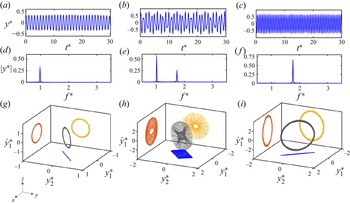
Figure 6 shows three sample displacement time histories (first row), and their corresponding frequency content (FFT plots at the second row) at three reduced velocities of  $U^*=6.05$,
 $9.21$ and
 $12.05$ for the eigenfrequency ratio of
 $R=1.7$. The time and frequency values in the
 $x$ axes are plotted as dimensionless values (
 $t^*$ and
 $f^*$), normalized by the first natural frequency of the system. The third row plots represent the periodic orbits in the 3-D space of
 $(y^*_1,y^*_2,\dot {y}^*_1)$, as those studied earlier in figure 4. These sample reduced velocities are selected such that they represent three different regions of modal contributions in the VIV response of the system; at the low reduced velocity of
 $U^*=6.05$, the VIV response of the system consists of oscillations occurring at pure mode one, represented with a single sharp peak at its frequency content (FFT) plot (figure 6d). At a higher reduced velocity of
 $U^*=9.21$, the VIV response of the system is a multi-modal response selected at the transition region from mode one to mode two, at which oscillations have contributions from both modes with two sharp peaks at values close to the first and second eigenfrequencies of the system (figure 6e). Finally, at the reduced velocity of
 $U^*=12.05$, the VIV response of the system consists of oscillations at the second structural mode, with frequency contents represented by a sharp peak at the frequency close to the second eigenfrequency of the system (figure 6f). The projections of periodic orbits (third row plots) on the
 $x$–
 $y$ plane confirm that indeed modes one and two are excited at a reduced velocity of
 $U^*=6.05$ and
 $U^*=12.05$, as they form an ellipse with
 ${+}45^{\circ }$ and
 ${-}45^{\circ }$ orientations, respectively. More importantly, the observed periodic orbits with a stretched rectangular form in the
 $x$–
 $y$ plane at the reduced velocity of
 $U^*=9.20$ assure that the observed VIV response is a multi-modal response where both modes one and two are excited.
Displacement time histories (a–c) and the corresponding FFTs (d–f) and periodic orbits (g–i) at the reduced velocity of  $U^*=6.05$ representing mode 1 (a,d,g),
 $U^*=9.20$ representing transition from mode 1 to mode 2 (b,e,h), and
 $U^*=12.05$ representing mode-2 oscillations (c, f,i).

4.2. Flow forces
An additional series of water tunnel experiments were conducted during which the force sensor was attached to the upper end of the cylinder, measuring the total flow forces acting on the cylinder in both the crossflow and inline directions as the cylinder undergoes VIV. The measured forces in the crossflow direction comprised both the hydrodynamic flow forces and the inertia force due to the motion of the force sensor. Therefore, the inertia force was removed from the total measured transverse force by post-processing the experimental data. When the force sensor was added at the top of the submerged cylinder, the mass ratio and the submerged length of the cylinder were kept constant compared with the experiments done without the force sensor attached, the results of which were reported in the previous section. This was achieved by adjusting the length and mass of the bracket connecting the cylinder to the force sensor, which was kept above the water level. However, the mechanical coupling between the sensor and the bracket holding the cylinder added to the flexibility of the system, such that at high reduced velocities beyond  $U^*\approx 16.0$, the cylinder in our experiments experienced shaking at its free end, causing the flow forces to take unrealistic values at such high reduced velocities. As a solution, an alternative method was used here to obtain the flow forces in the crossflow direction. This technique works based on using the time series of the cylinder's crossflow displacement to calculate and reconstruct the crossflow forces as
 $$\begin{gather} \left\{\begin{array}{c}
F_y \\ 0 \end{array}\right\}=\boldsymbol{{\boldsymbol{\mathsf{\Phi}}}}
{\boldsymbol{\mathsf{\Phi}}}^T\left\{\begin{array}{l} \ddot{y}_1 \\ \ddot{y}_2
\end{array}\right\}+{\boldsymbol{\mathsf{\Phi}}}\left[\begin{array}{cc} 2
\zeta_1 \omega_{n 1} & 0 \\ 0 & 2 \zeta_2 \omega_{n 2}
\end{array}\right] {\boldsymbol{\mathsf{\Phi}}}^T\left\{\begin{array}{l}
\dot{y}_1 \\ \dot{y}_2 \end{array}\right\}\nonumber\\
+\,{\boldsymbol{\mathsf{\Phi}}}\left[\begin{array}{cc} \omega_{n 1}^2 & 0 \\ 0 &
\omega_{n 2}^2 \end{array}\right]
{\boldsymbol{\mathsf{\Phi}}}^T\left\{\begin{array}{l} y_1 \\ y_2
\end{array}\right\}, \end{gather}$$
where  $F_y$ is the crossflow force acting on the cylinder,
 ${\boldsymbol{\mathsf{\Phi}}}$ is the mass-normalized mode shape of the system (obtained only for the structure, with no added mass contribution),
 $\omega _{ni}$ is the natural frequency of the system in air. Following the vibration models for discrete parameter systems (Inman & Singh Reference Inman and Singh1994), we have used a proportional viscous damping model to capture damping effects for the two DOF system. Assuming a proportional viscous model, we have measured the structural damping ratios at each mode of the system,
 $\zeta _i$, using free decay tests in air and have obtained similar damping ratios of
 $\zeta _1=\zeta _2=0.003$. Here,
 $y_i$ is the displacement data recorded using the non-contacting laser displacement sensor. This force reconstruction method was previously verified and used to measure the flow forces acting on a tapered cylinder and a triangular prism undergoing large amplitude flow-induced vibration (Seyed-Aghazadeh, Carlson & Modarres-Sadeghi Reference Seyed-Aghazadeh, Carlson and Modarres-Sadeghi2015, Reference Seyed-Aghazadeh, Carlson and Modarres-Sadeghi2017). Following this flow reconstruction technique, the reconstructed flow forces were shown to match very well with the results of the direct measurements using a force sensor during experiments (Seyed-Aghazadeh et al. Reference Seyed-Aghazadeh, Carlson and Modarres-Sadeghi2015). Here, sample cases are presented to show how this reconstruction method works for VIV response measurements of a two DOF circular cylinder.
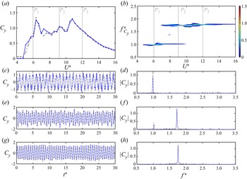
Figure 7(a,b) shows the comparison between the dimensionless crossflow force coefficients ( $C_y$) and their corresponding frequency content measured directly by the force sensor and those reconstructed using (4.1), plotted over the range of reduced velocities tested for a two DOF VIV case at the eigenfrequency ratio of
 $R=1.7$. The crossflow force coefficients are calculated as
 $C_y= 2 F_y/\rho D U^2 L$. Additionally, three sample cases of the crossflow force coefficient time histories and their corresponding frequency contents are plotted in figure 7(c–h) at sample reduced velocities of
 $U^*=6.05$,
 $9.21$ and
 $12.05$ (also shown with dashed lines in figures 7a,b). It is observed that the force reconstruction method not only is capable of reproducing the general force distribution over the range of reduced velocities tested, but also it can reproduce very fine details of the flow forces, as shown both in the time history and in the FFT plots of all three cases. Following this validation, the flow forces in the crossflow direction reported in this work are the reconstructed values, while the inline flow forces are directly measured via the force sensor, reported up to the reduced velocity of
 $U^*\approx 16$, at which the cylinder started to experience shaking. In addition, the force sensor measurements, as well as reconstructed crossflow forces, were synchronized with the displacement data recordings from the non-contacting displacement sensors, making it possible to directly obtain the phase difference between the flow forces and the displacement of the cylinder in the crossflow direction.
(a) Comparison between the crossflow force coefficients measured directly by the force sensor (grey dashed line) to those reconstructed using displacement data (blue solid line), (b) frequency content of the measured crossflow force coefficient, (c–g) time histories and (d–h) their corresponding frequency contents of the dimensionless crossflow forces at sample reduced velocities of  $U^*=6.05$,
 $9.21$ and
 $12.05$ at the eigenfrequency ratio of
 $R=1.7$.

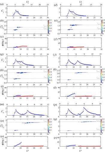
Figure 8 shows the crossflow force coefficients together with their frequency contents and phase differences between the flow forces and the displacement of the cylinder in the crossflow direction plotted against the reduced velocity for the VIV response of the cylinder with two DOF with varying eigenfrequency ratios. Shown with grey markers are the crossflow force coefficients for the VIV response of the cylinder with one DOF measured by the force sensor, plotted for comparison. The phase values are calculated based on filtering the displacement and force signals around the dominant frequency of oscillations. At the reduced velocity range at which multi-modal oscillations occur, the phase values are calculated by filtering the vibration response around each eigenfrequency of the system.
The crossflow force coefficients (first row), their corresponding frequency contents (second row), and the phase difference between the cylinder's displacement and the crossflow forces acting on the cylinder (third row) versus the reduced velocities of  $U^*$ and
 $U^*_2$ for all the eigenfrequency ratios tested. Plots are shown for the eigenfrequency ratio of
 $R=1.3$ (a–c),
 $R=1.5$ (d–f),
 $R=1.7$ (g–i),
 $R=2.1$ (j–l),
 $R=2.5$ (m–o) and
 $R=3.0$ (p–r). The grey markers show the crossflow force coefficients for the VIV response of a single DOF system.

At the eigenfrequency ratio of  $R=1.3$, the crossflow force coefficients increase sharply from zero at the beginning of the first VIV region to the maximum value of
 $C_y\approx 1.6$ at the reduced velocity of
 $U^*=6.4$. This trend, reduced velocity ranges and the maximum
 $C_y$ values stay the same for all the eigenfrequency ratios, following a very similar trend compared with those observed for the VIV response of a one DOF cylinder, shown in grey dashed lines. In this reduced velocity range that the crossflow force coefficients increase to their maximum values, the frequency content of the forces exhibits contributions from the first eigenfrequency of the system. As the reduced velocity is further increased, contributions from the second eigenfrequency of the system are observed in the frequency content plots of the crossflow forces. Once the multi-modal flow forces dominate the VIV response of the system, by increasing the reduced velocity the crossflow force coefficient decreases. The force coefficient values then exhibit a plateau, at which the force coefficients stay around the value of
 $C_y\approx 1.1$. As the reduced velocity further increases, the multi-modal response gives way to oscillations at the second mode. For this range of reduced velocity at the second lock-in region, the force coefficient values pick up again and reach to a second maxima. As the reduced velocity further increases, the force coefficients decrease and reach zero once the response exits the second lock-in region. The crossflow force coefficients have a relatively similar trend for all eigenfrequency ratios. As the eigenfrequencies take values further away from each other, the two peaks in the crossflow force coefficient plots grow separately from each other. For example, at the eigenfrequency ratio of
 $R=2.1$ and beyond, the two maxima peaks of the force coefficients are completely separated, where the first region with the corresponding maximum peak of the force coefficient occurs at the reduced velocity range of
 $U^*=4.8\unicode{x2013}10.8$ over which the VIV response is dominated by oscillations at the first mode. The second region is followed over the reduced velocity range of
 $U^*=10.8\unicode{x2013}23.8$, at which the second mode dominates the VIV response of the system. The overall force coefficient values in the first peak region, dominated by the first structural mode, closely match the force coefficients of those observed for the VIV response of a single DOF circular cylinder.
The phase difference between the crossflow displacements and forces plotted in the third row of figure 8 shows a change with reduced velocity for each eigenfrequency ratio. For eigenfrequency ratios below  $R=2.1$, for which the VIV response represents a multi-modal oscillation for an intermediate reduced velocity range during the transition from mode one to mode two, the phase values stay below
 ${\approx }12^\circ$ for the entire range of reduced velocities. This behaviour is different from what is observed in the VIV response of a circular cylinder, for which there is a phase jump from
 $0^\circ$ to
 $180^\circ$ between flow forces and the cylinder displacement (Khalak & Williamson Reference Khalak and Williamson1999). This is due to the fact that with a non-zero structural damping, the phase jump to
 $180^\circ$ occurs only if the frequency ratio between the oscillation frequency and the natural frequency of the system measured in air (
 $f_{osc}/f_{na}$) gets values far from unity (Sarpkaya Reference Sarpkaya2004). In the current experiments, however, the frequency ratio stays close to unity, resulting in a phase difference of less than
 $180^\circ$. The dashed lines in the frequency contents of the crossflow forces represent the first and second natural frequencies of the system in air. For eigenfrequency ratios of
 $R=2.1$ and
 $R=2.5$, there is a phase change from small values to values close to
 $45^\circ$ for the circular cylinder tested here, which means that the flow forces start opposing the displacement at a certain reduced velocity close to the end of the first lock-in region. Once the second mode oscillation starts to ramp up, the phase goes back to zero and it stays around values smaller than
 $5^\circ$ for the entire reduced velocity range over the second lock-in range.
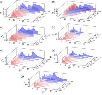
Figure 9 shows the overall VIV response of the circular cylinder, free to oscillate in two DOF in the crossflow direction, compared with those of a single DOF VIV response of a circular cylinder. The overall amplitude of oscillation versus reduced velocity is plotted in figure 9(a) for all the eigenfrequency ratios tested. As discussed earlier, by increasing the eigenfrequency ratio, the lock-in range gets extended to higher reduced velocities. Beyond a critical eigenfrequency ratio of  $R=2.1$, the lock-in region is split into two very separate regions, at which each eigenmode is excited, separately. The corresponding modal contributions versus the reduced velocities are plotted in figure 9(b) for the range of eigenfrequencies tested. The modal contributions exhibit oscillations that shift from pure mode one at low reduced velocities to a range of intermediate reduced velocities at which multi-modal oscillations occur. By increasing the reduced velocity values, the contributions from mode one decrease to zero and the VIV response gets dominated by pure mode two oscillations. While for the eigenfrequency ratios below
 $R=2.1$, the VIV response of the system follows this behaviour, for relatively larger eigenfrequency ratios of
 $R=2.5$ and 3.0, the two lock-in regions are well separated from each other such that there does not exist any intermediate reduced velocity range at which multi-modal oscillations occur. Time-averaged and fluctuating inline force coefficients are shown in figures 9(c) and 9(d), respectively. The inline force coefficients here are directly measured through the force sensor attached atop of the cylinder. The force coefficients are plotted for the reduced velocities up to which the cylinder does not experience any shaking at its tip. The time-averaged inline force coefficients evolution follows similar trends as those of the amplitude of oscillations at each eigenfrequency ratio, where they increase to a maximum value at the reduced velocity at which the maximum oscillation occurs, and decrease to lower values as the amplitude of oscillation decreases. As for fluctuating components of the inline force coefficients, while their maximum values appear to be relatively the same for a wide range of eigenfrequency ratios, multiple peaks are observed as the eigenfrequency ratios increase. The crossflow force coefficients shown in figure 9(e) increase from zero to their maximum values and decrease back to zero for a single DOF system, while they exhibit two maxima for a two DOF system. The two maxima get further away from each other as the eigenfrequency ratio gets larger. Figure 9( f,g) shows the crossflow force coefficients in phase with velocity (
 $C_{yv}$) and the crossflow force coefficients in phase with acceleration, known as the added mass coefficient (
 $C_{ma}$), versus the reduced velocity for all the eigenfrequency ratios, respectively. These values have been calculated as (Wang, Fan & Triantafyllou Reference Wang, Fan and Triantafyllou2021)
 \begin{equation} {C}_{y v}=\frac{2}{T_s}
\cdot \frac{\int_{T_s}\left(C_y(t) \dot{y}(t)\right)
\,{\rm d} t}{\sqrt{\frac{2}{T_s}
\int_{T_s}\left(\dot{y}^2(t)\right) \,{\rm d}t}},\quad {\rm
and}\quad {C}_{m a}={-}\frac{2 U^2}{{\rm \pi} {\rm d}^2} \cdot
\frac{\int_{T_s}\left(C_y(t) \ddot{y}(t)\right) \,{\rm d}
t}{\int_{T_s}\left(\ddot{y}^2(t)\right) \,{\rm d} t},
\end{equation}
where  $C_y$ is the instantaneous crossflow force coefficient,
 $T_s$ is one vibration cycle and the dots represent derivatives with respect to time. The calculated crossflow force coefficients in phase with velocity have all positive values for all the reduced velocities tested, confirming that the flow forces contribute to the excitation of the cylinder for all the cases studied here. The crossflow force coefficients in phase with velocity values also follow similar trends as those observed for the crossflow force coefficients, where two peaks are observed for the two DOF system. The distance between two maxima increases with the increase in eigenfrequency ratio. Figure 9(g) shows the crossflow force coefficients in phase with acceleration, known as the added mass coefficient (
 $C_{m_a}$), versus the reduced velocity for all the eigenfrequency ratios tested. These added mass coefficients have all positive values for all the reduced velocities tested. As shown previously (Wang et al. Reference Wang, Fan and Triantafyllou2021), the value of the added mass coefficient reflects the relative motion between the oscillating cylinder and the shed vortex in the near wake of the cylinder. This relation will be discussed further by studying the wake dynamics of the cylinder in the following section.
An overall comparison of the VIV response of the system in terms of its (a) dimensionless amplitude of oscillations, (b) modal contributions, (c) time-averaged inline force coefficients, (d) inline force coefficients, (e) crossflow force coefficients, ( f) crossflow force coefficients in phase with velocity and (g) crossflow force coefficients in phase with acceleration versus the reduced velocity for all eigenfrequency ratios.

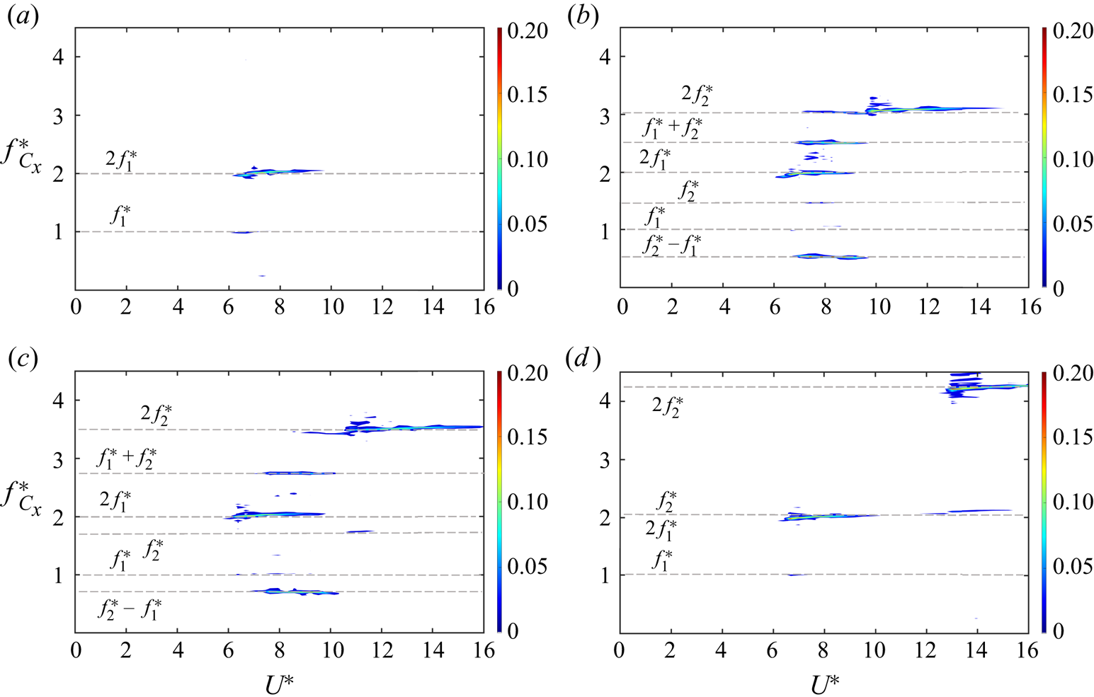
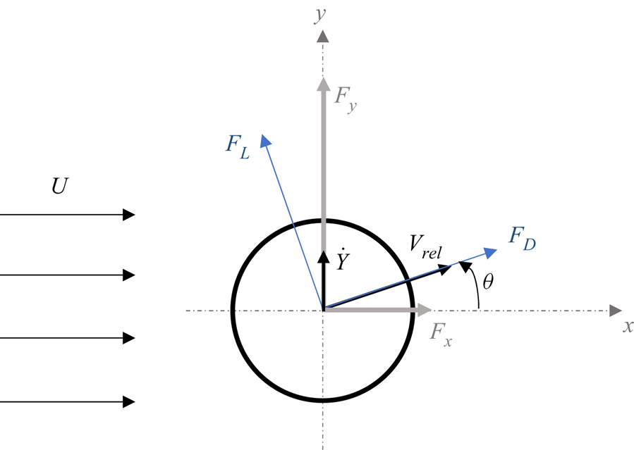
While in figure 9(d) we discussed the values of the inline force coefficients versus reduced velocity for the range of eigenfrequencies tested, it is also worth discussing their frequency contents here. Figure 10 represents the frequency contents of the inline force coefficients for the sample cases of a single DOF cylinder (figure 10a) and three eigenfrequencies of  $R=1.3, 1.7$ and 2.1 (figure 10b–d). For the single DOF system, the inline force coefficients follow a trend that is in agreement with previous VIV studies, for which the second harmonic frequencies, with values twice the natural frequency of the system, are observed as the dominant frequency, with small contributions from the first harmonic frequencies (Carlson, Currier & Modarres-Sadeghi Reference Carlson, Currier and Modarres-Sadeghi2021). When the cylinder is given the second DOF, the frequency content still exhibits the first and second harmonic contributions of each eigenfrequency. In addition to these frequencies, with two DOF oscillations additional frequencies are also present in the frequency contents shown in figure 10(b–d). These components are associated with the relative velocity of the cylinder moving in the crossflow direction that makes an angle with respect to the oncoming flow. Figure 11 shows the flow forces acting on an oscillating cylinder. As the cylinder oscillates, due to the relative velocity of the body with respect to the oncoming flow, the lift and drag forces make an angle with respect to the crossflow and inline directions. Previous VIV studies have shown the existence of second and third harmonic frequency components in the flow forces, when the cylinder was free to oscillate in the crossflow direction (Du, Jing & Sun Reference Du, Jing and Sun2014; Seyed-Aghazadeh et al. Reference Seyed-Aghazadeh, Carlson and Modarres-Sadeghi2015). Of particular interest in the current study is the frequency contents of the inline flow forces at the eigenfrequency ratios for which the VIV response of the system exhibits multi-modal oscillations over a range of reduced velocities. Assuming sinusoidal multi-modal oscillations for the cylinder in the inline direction as
 \begin{equation} Y(t)=Y_{1} \sin \left(\omega_{1} t\right) + Y_{2} \sin \left(\omega_{2} t\right), \end{equation}
in which  $\omega _1$ and
 $\omega _2$ are the two frequencies of cylinder oscillation and
 $Y(t)$ is the dimensionless amplitude of oscillation with respect to the diameter of the cylinder,
 $D$. The flow forces acting in the inline direction can be expressed as
 \begin{equation} F_{x}(t)=F_{D}(t) \cos \theta-F_{L}(t) \sin \theta, \end{equation}
where  $F_L$ and
 $F_D$ are the lift and drag forces with combined frequencies of
 $\omega _1$ and
 $\omega _2$ and the values twice those, respectively, which can be expressed as
 \begin{gather} F_{L}(t)=F_{L 1} \sin \left(\omega_{{1}} t+\psi_{1}\right) + F_{L 2} \sin \left(\omega_{{2}} t+\psi_{2}\right), \end{gather}
 $$\begin{gather} F_D(t)=\bar{F}_D+F_{D 1} \sin \left(\omega_1 t+\psi_3\right)+F_{D 2} \sin \left(\omega_2 t+\psi_4\right)+F_{D 3} \sin \left(2 \omega_1 t+\psi_5\right)\nonumber\\ +F_{D 4} \sin \left(2 \omega_2 t+\psi_6\right), \end{gather}$$
where  $\psi$ values are the phase angles between the lift and drag forces with respect to the cylinder's displacement. It is worth noting that ideally, for a symmetric wake of the cylinder, one would expect the drag force frequency content to include only frequencies twice those observed in the lift direction. However, in general, any asymmetry of the wake can lead to frequency contents at similar values of those in the lift forces and their corresponding second harmonics, as those considered here in (4.6) (Carlson et al. Reference Carlson, Currier and Modarres-Sadeghi2021). For a small angle between the flow velocity and the relative velocity,
 $\theta$,
 \begin{equation} \sin \theta \sim \tan \theta \sim \dot{Y}, \quad \cos \theta \sim 1, \end{equation}
where  $\dot {Y}$ is the dimensionless velocity of the cylinder in the crossflow direction. Following the assumption of a small angle
 $\theta$, (4.4) can be written as
 \begin{equation} F_{x}(t)=F_{D}(t)-F_{L} \dot{Y}(t). \end{equation}
Frequency contents of the inline force coefficients for (a) the sample case of a single DOF cylinder, and (b–d) three eigenfrequencies of  $R=1.3, 1.7$ and 2.1.

Flow forces acting on a cylinder undergoing VIV.

Substituting the lift and drag forces from (4.5) and (4.6), as well as  $\dot {Y}$ in the form of
 $\dot {Y}=Y_{1} \omega _{{1}} \cos (\omega _{{1}} t)+ Y_{2} \omega _{{2}} \cos (\omega _{{2}} t)$ in (4.8), the flow force coefficient,
 $C_{x}(t)=2 F_{x} / \rho D U^{2} L$, in the inline direction can be obtained as
 $$\begin{align} C_x(t) &= C_1 \sin
\left(\omega_1 t+{\boldsymbol{\mathsf{\Phi}}}_1\right)+C_2 \sin \left(\omega_2
t+{\boldsymbol{\mathsf{\Phi}}}_2\right)+C_3 \sin \left(2 \omega_1
t+{\boldsymbol{\mathsf{\Phi}}}_3\right)+C_4 \sin \left(2 \omega_2 t+{\boldsymbol{\mathsf{\Phi}}}_4\right)
\nonumber\\ &\quad+\,C_5\left(\sin \left(\omega_1+\omega_2\right)
t+{\boldsymbol{\mathsf{\Phi}}}_5\right)+C_6\left(\sin
\left(\omega_1-\omega_2\right) t+{\boldsymbol{\mathsf{\Phi}}}_6\right),
\end{align}$$
in which  $C_1$–
 $C_6$ are functions of the lift and drag coefficients, frequencies of oscillations and the phase difference between the flow force and the cylinder displacement. As expressed in (4.9), the flow force in the inline direction consists of the first and second frequencies and their second harmonics (terms with
 $\omega _1$ and
 $\omega _2$ and values twice those), as well as other harmonics with frequencies of
 $(\omega _1+\omega _2)$ and
 $(\omega _1-\omega _2)$. These frequency contents are shown for the sample cases in figure 10(b,c) for the two cases at which the oscillations exhibit multi-modal behaviour over a range of reduced velocities. For the single DOF system as well as the two DOF at the eigenfrequency of
 $R=2.1$, the oscillations of the cylinder exhibit a mono-frequency oscillation and, therefore, only the dominant frequencies and their second harmonics at values twice the system's natural frequencies are observed. An advantage of having a two DOF set-up to study the VIV response of the cylinder shows itself here as it has enabled us to observe, identify and discuss the existence and the source of multiple frequency components in the VIV system of the circular cylinder in our study in a straightforward fashion. These frequencies often remain unnoticed when we study the complex multi-modal VIV response of a flexible cylinder, for which the complexity of the response makes it very challenging and difficult to separately study the frequency contents of the response as we did here and they mostly remain unidentified or not discussed.
4.3. Wake structure
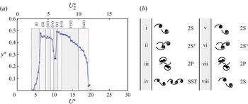
An overall map of shedding patterns observed in the wake of the circular cylinder undergoing VIV in two DOF at the sample eigenfrequency ratio of  $R=1.7$ is given in figure 12. This sample eigenfrequency ratio has been selected such that the cylinder exhibits mono-frequency oscillations at each of its first two eigenfrequencies over a range of reduced velocities, and also experiences multi-modal oscillations over a range of reduced velocity over which the VIV response of the system shifts from oscillations at the dominant mode one to oscillations dominated by the second eigenfrequency of the system. The predominant shedding patterns at lower reduced velocities, for which the VIV enters the first lock-in region, are symmetric two single vortices shed per one cycle of oscillations, known as
 $2S$ shedding (region i), that later transition to an asymmetric
 $2S$ shedding as the amplitude of oscillation reaches the maximum amplitude (region ii). The asymmetry into the shedding is introduced as a shear layer from one side of the cylinder gets stretched and entrained into the wake of an already shed single vortex from the opposite side of the cylinder. The asymmetric
 $2S$ shedding later develops into two pairs of vortices being shed per cycle of oscillation, known as
 $2P$ vortex shedding. The
 $2S$ and its transition to
 $2P$ shedding have been observed previously for the VIV response of a circular cylinder with a single DOF to oscillate in the crossflow direction (Govardhan & Williamson Reference Govardhan and Williamson2000). As the reduced velocity is further increased, the oscillations enter an overlapping range at which both eigenfrequencies dominate the VIV response of the system (region iv). At this range of reduced velocity, the shedding pattern per one cycle of oscillations exhibits two single vortices being shed followed by a triplet of vortices, named here as
 $SST$ shedding. Once the VIV response enters the second lock-in region at which the oscillations are dominated by the second eigenfrequency of the system, similar vortex shedding patterns as those observed in the first lock-in region repeat themselves, i.e.
 $2S$ vortex shedding patterns at lower reduced velocity (region v), that transition to
 $2P$ patterns at region (vii) through an asymmetric
 $2S$ shedding pattern observed in region (vi). At high reduced velocity the VIV response of the system drops to lower amplitudes and the response exits the second lock-in region (region viii), the shedding pattern exhibits a
 $2S$ vortex shedding.
(a) A map of the vortex patterns in the wake of the cylinder at the eigenfrequency ratio of  $R=1.7$ at different reduced velocities, together with (b) schematics of the shedding patterns.

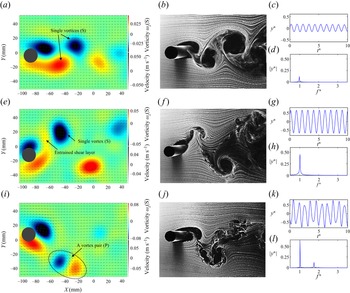
Figure 13 shows the vortex shedding patterns in the wake of the cylinder using PTV and hydrogen bubble flow visualization, together with the time histories and frequency content (FFT plots) of the VIV response of the cylinder at sample reduced velocities of  $U^*=5.4, 6.7$ and 7.9. The snapshots on the left (the first column) are the instantaneous out-of-plane vorticity plots obtained through the time-resolved 3-D PTV measurements, as discussed in § 2 and the snapshots at the right are directly from hydrogen bubble flow visualization (the second column). The vorticity plots are taken at a normalized spanwise submerged length of
 $z=0.5$, measured from the free bottom end of the cylinder. The time histories and their corresponding frequency contents shown on the third column are plotted against dimensionless time and frequency, where the first eigenfrequency of the system is used to obtain those values as
 $f^*=f_{osc}/f_N$ and
 $t^*=t \times f_N$. The sample reduced velocities are selected such that they represent all the possible shedding patterns that could occur over the first lock-in region, as discussed earlier in figure 12. The hydrogen bubble flow visualization videos at these reduced velocities are also provided as electronic supplementary movies 1–3 available at https://doi.org/10.1017/jfm.2022.893. At the reduced velocity of
 $U^*=5.4$, two single vortices are shed per one cycle of oscillations (
 $2S$ pattern). The vortex shedding frequency at this reduced velocity is equal to the frequency of oscillations (
 $f_{vs} =f_{osc} =0.46$ Hz at
 $U^*=5.4$), which is a feature of a VIV response. The frequency content of the response exhibits a single peak at the dimensionless frequency close to unity, that represents a mono-frequency oscillation at values close to the first eigenfrequency of the system. At the reduced velocity of
 $U^*=6.7$, the
 $2S$ vortex shedding pattern persists, but the shedding loses its symmetry, such that once a vortex is shed from one side of the cylinder a shear layer from the other side of the cylinder gets wound around the already shed vortex. As the cylinder moves to the opposite side, a second vortex is fully shed. The extended shear layer from the bottom of the cylinder gets wound around the shed vortex from the top, as also presented in the vorticity field measurements shown in figure 13(e). The time history and the frequency content of the VIV response at this reduced velocity still exhibit a mono-frequency oscillation at a frequency close to the first eigenfrequency of the system. At the reduced velocity of
 $U^*=7.9$, the response is still in the first lock-in region and the shedding pattern observed in the wake of the cylinder exhibits a pair of vortices being shed per one cycle of oscillation (
 $2P$ shedding). The pairs are both observed in the hydrogen bubble flow visualization and the vorticity plots of figure 13. The time histories and the frequency content at this reduced velocity exhibits a multi-modal oscillation; while the response is dominated by a frequency of oscillation at the first eigenfrequency of the system, small contributions from the second eigenfrequency of the system are observed at the dimensionless frequency of
 $f^*=1.7$. The time histories also exhibit their deviation from a single harmonic oscillatory response to a periodic oscillation with more than one frequency.
Vortex shedding patterns in the wake of the cylinder using out-of-plane vorticity plots obtained through the time-resolved 3-D PTV measurements (a,e,i), and hydrogen bubble flow visualization (b, f,j), together with the time histories and frequency content (FFT plots) of the VIV response of the cylinder (c,d,g,h,k,l) at sample reduced velocities of  $U^*=5.4$ (a–d), 6.7 (e–h) and 7.9 (i–l). The videos are provided as supplementary movies 1–3.

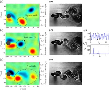
Figure 14 shows the shedding patterns at three sample time stamps in one cycle of oscillation of the cylinder, followed by the oscillation time histories and frequency content at the reduced velocity of  $U^*=9.8$. This is a sample reduced velocity from region (iv) of figure 12 at which the VIV response of the system is dominated by comparable contributions from both eigenfrequencies of the system. The vortex shedding at this region exhibits a unique pattern; in one full cycle of oscillation the cylinder sheds two single vortices followed by a triplet of vortices (
 $SST$). This shedding pattern and the time stamps at which each shedding occurs are presented in figure 14. The hydrogen bubble flow visualization video is also provided as electronic supplementary movie 4.
Vortex shedding patterns in the wake of the cylinder using out-of-plane vorticity plots obtained through the time-resolved 3-D PTV measurements (a,c,g), and hydrogen bubble flow visualization (b,d,h), together with the time histories and frequency content (FFT plots) of the VIV response of the cylinder (e, f) at sample reduced velocity of  $U^*=9.8$ at three time stamps during one cycle of oscillation of
 $t_1$ (a,b),
 $t_2$ (c–f) and
 $t_3$ (g,h). The video is provided as supplementary movie 4.

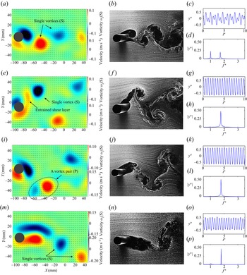
Figure 15 shows the shedding patterns and the oscillation time histories and frequency content at the reduced velocities of  $U^*=10.1, 11.1, 13.0$ and
 $17.7$. At the reduced velocity of
 $U^*=10.1$, that is, a sample reduced velocity from region (v) from figure 12, the VIV response of the system is dominated by comparable contributions from both eigenfrequencies of the system. This region coincides with the onset of the second lock-in region and the wake exhibits two single vortex shedding patterns per one cycle of oscillation (
 $2S$). The
 $2S$ shedding pattern resembles those previously seen at the onset on the first lock-in range in region (i). The vortex shedding frequency at this point is equal to the frequency of oscillations in the second eigenfrequency (
 $f_{vs} =f_{osc} =0.82$ Hz at
 $U^*=10.1$), which is a feature of a VIV response. At the reduced velocity of
 $U^*=11.1$, that is, a sample reduced velocity from region (vi) from figure 12, mono-frequency oscillations are observed at which the VIV response of the system exhibits frequency contents at values close to the second eigenfrequency of the system. The wake of the cylinder exhibits an asymmetric
 $2S$ vortex shedding pattern, where similar to region (ii) in the first lock-in region, the symmetry of the two single vortices are broken. At the reduced velocity of
 $U^*=13$, that is, a sample reduced velocity from region (vii) of figure 12, the vortex shedding patterns follow the same trend as those observed in the first lock-in region where the asymmetric
 $2S$ shedding transitions to the
 $2P$ shedding pattern. The frequency content of the dynamic response of the system exhibits mono-frequency oscillations at a value close to the second eigenfrequency of the system. Finally, at the reduced velocity of
 $U^*=17.7$, that is, a sample reduced velocity from region (viii) of figure 12, the amplitude of oscillations decreases to smaller values that mark the end of the second lock-in region. At this reduced velocity the wake of the cylinder exhibits a very turbulent
 $2S$ vortex shedding pattern. The PTV measurements represent two elongated shear layers being shed from each side of the cylinder.
Vortex shedding patterns in the wake of the cylinder using out-of-plane vorticity plots obtained through the time-resolved 3-D PTV measurements (a,e,i,m), and hydrogen bubble flow visualization (b, f,j,n), together with the time histories and frequency content (FFT plots) of the VIV response of the cylinder (a,d,g,h,k,l,o,p) at sample reduced velocities of  $U^*=10.1$ (a–d), 11.1 (e–h), 13.0 (i–l) and 17.7 (m–p).

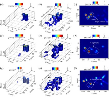
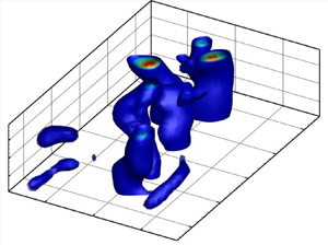
We would like to expand the wake structure discussion by pointing out the 3-D nature of the wake of the cylinder undergoing VIV in our study. While the wake snapshots shown in figures 13–15 have been taken at one spanwise location ( $z=0.5$) along the length of the cylinder, our time-resolved volumetric PTV measurements can provide insights into the 3-D wake of the cylinder. To acquire further details of the vortex structures, the Q criterion was implemented using both the time-averaged and instantaneous vector fields. The Q criterion is defined as (Hunt, Wray & Moin Reference Hunt, Wray and Moin1988)
 \begin{equation} Q= \frac{(\|\varOmega\|^2 - \|S\|^2)}{2}, \end{equation}
where  $\varOmega$ and
 $S$ represent vorticity and strain rate in the flow field, respectively. Positive
 $Q$ values in the flow field indicate places where vorticity reigns supreme. Samples of the normalized volumetric and two-dimensional (2-D) Q criterion are represented in figure 16 at three sample reduced velocities of
 $U^*=$ 5.4, 9.8 and 13 for the eigenfrequency ratio of
 $R=1.7$. Positive values of
 $Q$ distinguish dominant vortices in the wake of the cylinder. The time-averaged volumetric Q-criterion plots (first column plots) show spanwise change in the location of the shed vortex along the length of the cylinder, indicating that the vortical structures in the wake of the cylinder undergoing VIV have a 3-D nature. The three-dimensionality effects get more dominant at higher reduced velocities, as those shown in figure 16(e,h). While the wake exhibits a 3-D behaviour, it is worth noting that the very same vortex shedding patterns discussed earlier in figure 12 still dominate the wake of the cylinder. Figure 16(e, f) shows instantaneous
 $Q$ for a reduced velocity of
 $U^*=9.8$, for which the vortex shedding patterns were observed to be of
 $SST$-type (figure 14). A triplet and two single vortices are observed in the wake of the cylinder at the instantaneous
 $Q$ contour at this reduced velocity. However, the triplet vortices are not observed in the time-averaged Q-criterion contour (figure 16d). This can be explained by the fact that the trailing triplet vortices in the wake of the cylinder are weaker than the leading two single vortices in the repeated shedding pattern, resulting in dominant 2
 $S$ patterns observed in the time-averaged contour. At the reduced velocity of
 $U^*=13$, the 2-D and 3-D instantaneous Q-criterion contours show the dominant
 $2P$ vortex shedding patterns in the wake of the cylinder, as also expected from previous observations in figure 12. Since the shed vortices are advected downstream, the
 $2P$ vortex shedding pattern is no longer present in the time-averaged Q-criterion contour (figure 16g).
Time-averaged 3-D (a,d,g), instantaneous 3-D (b,e,h) and 2-D (c, f,i) normalized Q-criterion contours at reduced velocities of  $U^*=5.4$ (a–c),
 $U^*=9.8$ (d–f) and
 $U^*=13$ (g–i).

4.4. Proper orthogonal decomposition
Proper orthogonal decomposition is one of the most robust techniques to investigate the turbulent flow's large (energetic) coherent structures (Berkooz, Holmes & Lumley Reference Berkooz, Holmes and Lumley1993; Lumley Reference Lumley2007; Sieber, Paschereit & Oberleithner Reference Sieber, Paschereit and Oberleithner2016; Taira et al. Reference Taira, Brunton, Dawson, Rowley, Colonius, McKeon, Schmidt, Gordeyev, Theofilis and Ukeiley2017). The unsteady flow field,  $\boldsymbol{u}$, could be represented as a long-time mean field,
 $\bar {U}$, and fluctuation flow,
 $\boldsymbol{u}^\prime$, via the general Reynolds decomposition as
 \begin{equation} \boldsymbol{u}=\bar{U}+\boldsymbol{u}^\prime. \end{equation}
In the current study, the method of snapshots POD introduced in Sirovich (Reference Sirovich1987) is used to present the fluctuation of a vector field using a linear combination of orthonormal modes to solve an eigenvalue problem. The snapshots approach decomposes the time-dependent fluctuation velocity field,  $\boldsymbol{u}_i^\prime (x,t)$, into the unsteady spatial basis functions of
 ${\boldsymbol{\mathsf{\Phi}}} _k (x)$ and their corresponding temporal modal coefficients of
 $a_k (t)$ as
 \begin{equation} \boldsymbol{u}_i^\prime(x,t)= \sum_{k=1}^{N} a_k(t){\boldsymbol{\mathsf{\Phi}}}_k(x), \end{equation}
with  $N$ being the number of snapshots employed in the calculation. In the current study, the POD method is applied to the resulting 3-D velocity field obtained via the time-resolved 3-D PTV measurements. To obtain spatial (
 ${\boldsymbol{\mathsf{\Phi}}} _k(x)$) and temporal (
 $a_k (t)$) POD modes, single value decomposition (SVD) was applied to the fluctuation velocity field
 $(\boldsymbol{u}-\bar {U})$) as (Horn & Johnson Reference Horn and Johnson1985; Trefethen & Bau Reference Trefethen and Bau1997; Saad Reference Saad2011):
 \begin{equation} ({\boldsymbol{\mathsf{\Phi}}}, \sqrt{\lambda}, a) = \text{SVD}(\boldsymbol{u}-\bar{U}), \end{equation}
where the eigenvalues  $\lambda$ represent the collected energy from POD modes
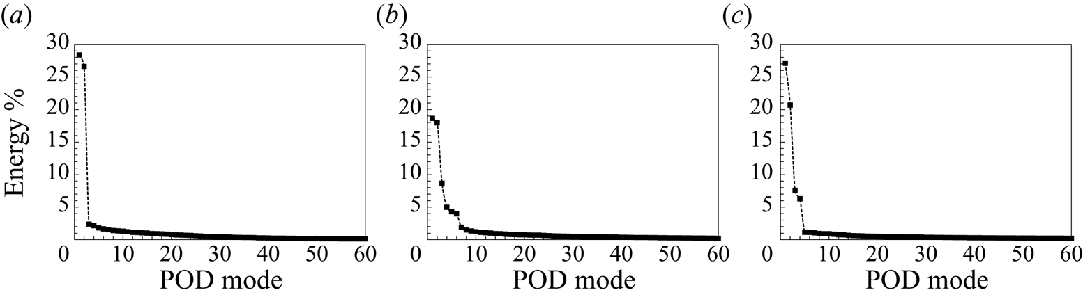
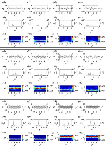
 ${\boldsymbol{\mathsf{\Phi}}} (x)$. A zeroth mode is assumed for the time-averaged flow field, which is then subtracted from each flow field signal. Figure 17 shows each mode's relative kinetic energy contribution as a percentage of the total energy at the three sample reduced velocities studied before. In the current work, to identify unstable wake flow by POD, the criteria to decide the number of contributing modes is set at
 $5\,\%$ of the total energy of modes. It is shown that the first few modes contribute to the majority of energy of the system in the samples reduced velocities selected, whereas the energy proportion of higher modes steadily drops to zero. In this study, the first four POD modes, containing higher than
 $5\,\%$ of the total energy levels, have been selected to be investigated in the following section.
Energy distribution for the first 60 POD modes at the reduced velocities of (a)  $U^*=5.4$, (b)
 $U^*=9.8$ and (c)
 $U^*=13$.

The three-dimensional spatial structure and corresponding temporal coefficients of the first four POD modes in terms of the streamwise and transverse velocity components at the three selected sample reduced velocities of  $U^*= 5.4, 9.8$ and
 $13$ at the eigenfrequency ratio of
 $R = 1.7$ are shown in figures 18–20, respectively. The sample reduced velocities are selected such that three distinct regions of the modal contributions to the VIV response of the system, i.e. pure modes one and two and the multi-modal VIV response, are covered. As figure 17 shows, at the reduced velocity of
 $U^*=5.4$, where the
 $2S$ shedding pattern was identified, the first two POD modes contain a dominant percentage of the total energy (
 $55\,\%$), and the third and fourth had less than
 $3\,\%$ energy. However, at the reduced velocities of
 $U^*=9.8$ and 13, at which the
 $SST$ and
 $2P$ shedding patterns were identified, while the first two POD modes contain approximately
 $36\,\%$ and
 $48\,\%$ of the total energy of the system, respectively, the third and fourth POD modes are still energetic with contributions of around
 $14\,\%$ to the total energy of the system. Figure 20 shows the corresponding temporal evolution of the first four POD modes at the same sample reduced velocities versus dimensionless time (figures 20
 $a1$–
 $a4$,
 $b1$–
 $b4$ and
 $c1$–
 $c4$), together with their frequency content shown through FFT plots (figures 20
 $a5$–
 $a8$,
 $b5$–
 $b8$ and
 $c5$–
 $c8$). The time and frequency in these plots are normalized by the system's first natural frequency. Scalogram plots (figures 20
 $a9$–
 $a12$,
 $b9$–
 $b12$ and
 $c9$–
 $c12$), obtained using the wavelet transform of the associated temporal coefficients time series, show the time evolution of the frequency contents normalized by the system's first natural frequency, that is plotted against the dimensionless time,
 $t^*$.
Spatial structures of the streamwise velocity for the first four POD modes (shown in each column from mode one to four) at the reduced velocities of  $U^*=5.4$ (a–d),
 $U^*=9.8$ (e–h) and
 $U^*=13$ (i–l).

Spatial structures of the transverse velocity for the first four POD modes (shown in each column from mode one to four) at the reduced velocities of  $U^*=5.4$ (a–d),
 $U^*=9.8$ (e–h) and
 $U^*=13$ (i–l).

Time evolution of the first four temporal coefficients ( $a_1$–
 $a_4$), their corresponding frequency contents (FFT plots) and scalogram plots at the reduced velocities of
 $U^*=5.4$ (box 1 – rows 1–3),
 $U^*=9.8$ (box 2 – rows 4–6) and
 $U^*=13$ (box 3 – rows 7–9). Dotted lines in the time histories and FFT plots represent the cylinder's amplitude of oscillations (
 $y^*$) and their frequency contents (
 $|y^*|$), respectively, at the corresponding reduced velocities.

The first sample reduced velocity of  $U^*= 5.4$ is selected at the region where the VIV response of the system experiences oscillations at only mode one (figures 18 and 19a–d). The first and second POD modes show the analogous spatial structures and shift to the downstream in the streamwise direction. Furthermore, the first and second POD modes illustrate the travelling wave's spatiotemporal structure, which is created as a result of vortices being shed from each side of the cylinder to the downstream. Asymmetric and symmetric patterns about the centreline of the spatial structure are observed in the first two modes in the streamwise and spanwise directions, respectively. Asymmetric velocity field distributions around the centreline indicate symmetric vorticity contour distributions, whereas symmetric patterns represent the mirrored symmetric ones (Konstantinidis, Balabani & Yianneskis Reference Konstantinidis, Balabani and Yianneskis2007). Therefore, the first two POD modes at this reduced velocity represent a symmetric
 $2S$ vortex shedding pattern. Figure 20(
 $a1$,
 $a2$,
 $a5$,
 $a6$) also shows the time history and FFT analysis of temporal coefficients for the first two modes at this reduced velocity. These coefficients fluctuate with a single frequency content with a sharp peak at the dominant frequency (
 $f^*=1)$, that is the same as the cylinder's first natural frequency, as shown in the frequency contents of FFT plots. This frequency corresponds to the vortex shedding frequency at this reduced velocity, that is also the same as the cylinder's oscillation frequency (shown with dotted lines). In contrast, the third and fourth POD modes show irregular spatial (figures 18 and 19c,d) and temporal patterns (figure 20
 $a3$,
 $a4$,
 $a7$,
 $a8$) associated with small-scale turbulent structures that exhibit several low-frequency peaks in the frequency content of the temporal coefficient modes. The scalograms of the associated temporal coefficient modes also show that, for the first and second modes, the vortex shedding frequency stays close to the first natural frequency of the cylinder during the oscillation (figure 20
 $a9$,
 $a10$). On the other hand, for the third and fourth temporal coefficients with lower levels of energy, the frequency contents are smaller than the cylinder's first natural frequency and they show temporal fluctuations in their frequency contents (figure 20
 $a11$,
 $a12$).
The second sample reduced velocity of  $U^*= 9.8$ is selected such that the VIV response of the system exhibits multi-modal oscillations that transition from oscillations at mode one to mode two. The two sharp peaks in the frequency content of the structure's oscillation response shown by the dotted lines in the FFT plots (figure 20
 $b5$–
 $b8$) represent such a multi-modal response with contributions from both modes with oscillation frequencies at the values close to the first and second natural frequencies of the system. The first two POD modes (figures 18 and 19e–h) represent almost identical structures of vortex shedding. As previously shown in figure 14, at this reduced velocity the wake exhibited the
 $SST$ shedding pattern. Analysing the POD modes here, it is observed that the first two POD modes behave similar to those at the reduced velocity of
 $U^*=5.4$, at which the 2
 $S$ vortex shedding pattern was observed. On the other hand, the third and fourth POD modes are significantly different. The third spatial structure in the streamwise direction shows nearly two parallel vortical structures, whereas the fourth POD mode exhibits uneven small-scale turbulence structures as the energy level at this mode is relatively low (figure 17). Additionally, the symmetric spatial pattern, as observed for the first two POD modes, is replaced with an erratic pattern in the transverse direction of the third and fourth POD modes. Similarly, corresponding temporal coefficients show the multi-modal behaviour in which the dominant frequency for the first and second temporal modes is close to the cylinder's second natural frequency (figure 20
 $b1$,
 $b2$,
 $b5$,
 $b6$). In contrast, the time history and frequency contents of the third and fourth temporal modes show that the dominant vortex shedding frequency is close to the cylinder's first natural frequency (figure 20
 $b3$,
 $b4$,
 $b7$,
 $b8$). Such a behaviour confirms that the first two modes with the highest energy levels (figure 17b) and high shedding frequency can be associated with the shedding of single vortices while the third mode with the moderate level of energy and low frequency (close to system's first natural frequency) corresponds to the shedding of triplet vortices. The fourth mode with a relatively lower energy level and low frequency can be associated with the small-scale turbulence structures in the wake of the cylinder. The scalograms, representing the time evolution of frequency content for the temporal coefficients, confirm the multi-modal oscillations of the first four temporal coefficient at the reduced velocity of
 $U^*= 9.8$ with the shedding frequency values close to the cylinder's first and second natural frequencies (figure 20
 $b9$–
 $b12$).
The third sample reduced velocity of  $U^*= 13$ is selected such that the VIV response of the system exhibits oscillations at the second structural mode, with the frequency content represented by a sharp peak near the system's second natural frequency (shown by dotted lines in figure 20
 $c5$–
 $c8$). The third row figures (figures 18–19i–l) show spatial patterns of the first four POD modes at this sample reduced velocity. The first two POD modes in the streamwise and transverse directions show similar asymmetric and symmetric vortical structures, respectively. The spatial structure of the third and fourth POD modes exhibits two small-scale parallel structures with opposing signs that are asymmetric in both the streamwise and transverse directions. The temporal POD modes at this reduced velocity show a mono-frequency behaviour in which frequency contents and the corresponding time evolution for the first two temporal coefficients (figure 20
 $c1$,
 $c2$,
 $c5$,
 $c6$) show a strong peak with its value close to the system's second natural frequency. The dominant frequency is doubled for the third and fourth POD modes compared with the first and second temporal modes (figure 20
 $c3$,
 $c4$,
 $c7$,
 $c8$). As suggested by previous studies (Konstantinidis et al. Reference Konstantinidis, Balabani and Yianneskis2007), these POD modes are attributed to the
 $2P$ symmetrical vortex structures in the wake of the cylinder. Scalogram plots at this reduced velocity indicate that the frequency of the first and second temporal mode coefficients stays close to the system's second natural frequency over time (figure 20
 $c9$,
 $c10$), and doubles for the third and fourth coefficients (figure 20
 $c11$,
 $c12$).
In summary, the aforementioned spatiotemporal mode analysis using the POD technique shows that vortex shedding modes in the wake of the cylinder are strongly coupled with the structural vibration modes, as discussed earlier in § 4.1. Both approaches of wavelet transform and the POD produced a strikingly similar frequency content for the structural oscillations response and the vortex shedding in the wake of the cylinder, in which the peak frequencies for the 3-D POD modes are well in agreement with those reported in the frequency analysis of the structural VIV response. Here, we demonstrated that the 3-D POD technique can well capture the proper vortex shedding modes and their corresponding frequency contents for a circular cylinder undergoing VIV. The POD technique used in conjunction with the structural response analysis techniques in our study provided us with a unique tool to better understand the VIV response of a circular cylinder and the associated complex and 3-D vortex dynamics in the wake of the cylinder. These combined techniques have potentials to be extended to studies of complex fluid–structure interaction systems, for which a strong coupling between the structural response and the surrounding complex and 3-D fluid flow exists.
5. Conclusion
An experimental study of VIV of a flexibly mounted rigid cylinder, free to oscillate in the crossflow direction at its first two modes, was conducted.
Dynamic response of the cylinder, in terms of amplitude of oscillations, flow forces and wake structures were studied for a range of reduced velocities of  $U^*=4\unicode{x2013}30$, corresponding to a Reynolds number range of
 $Re=1033\unicode{x2013}7478$ for a range of eigenfrequency ratios of the system. The VIV response of the system was shown to be heavily dependant on the ratio between the first two natural frequencies of the system and how far away they are from each other; for frequency ratios as small as
 $R=1.3$, the onset of the VIV response of the system was very similar to that observed for a classical VIV response of a single DOF circular cylinder. However, the lock-in width was extended to higher reduced velocities as the frequency ratios increased. The extended lock-in range was split between two regions where, for the first region at low reduced velocities, mono-frequency oscillations at the first mode were observed. As the reduced velocity was increased, the VIV response of the system transitioned to a range at which multi-modal oscillations dominated the response of the system. By further increasing the reduced velocity, the second lock-in region was observed, over which the VIV response of the system was dominated by the mono-frequency excitation at the second mode of the system. The modal contributions also exhibited oscillations that shifted from pure mode one at low reduced velocities to a range of intermediate reduced velocities at which multi-modal oscillations occurred. By increasing the reduced velocity values, the contributions from mode one decreased to zero and the VIV response got dominated by pure mode two oscillations. While, for the eigenfrequency ratios below
 $R=2.1$, the VIV response of the system followed this behaviour, for relatively larger eigenfrequency ratios of
 $R=2.5$ and 3.0, the two lock-in regions were well separated from each other such that there did not exist any intermediate reduced velocity range at which multi-modal oscillations occurred.
The crossflow and inline flow force coefficients were also studied for the range of reduced velocities and eigenfrequency ratios tested here. The crossflow force coefficients followed similar trends to those observed for the amplitudes of oscillation where their values increased to a maximum at reduced velocities where maximum oscillations occurred. By further increasing the reduced velocity, the flow force coefficients were dropped in their values at the transition region between mode one and mode two. At the reduced velocity range over which the second mode started to dominate the response of the system, the crossflow force coefficients picked up in their magnitudes and reached a second maximum value. By further increasing the reduced velocity, when the VIV response of the system dropped to lower amplitudes and exited the lock-in region, the crossflow force coefficient followed a similar decrease in value and got to zero when the oscillations stopped. In the inline direction, flow forces consisted of frequencies at the values close to the system's natural frequencies and their corresponding second harmonics, as expected from the classical VIV response of a single DOF system. However, for the range of reduced velocities and eigenfrequencies that the VIV response of the system exhibited multi-modal oscillations, other frequency components were also present in the frequency content of the inline forces. Existence of such harmonics were studied and related to the relative velocity of the cylinder as it underwent a multi-frequency VIV response.
Both qualitative and quantitative flow visualization tests were conducted to study vortex dynamics in the wake of the cylinder. For qualitative flow visualization purposes, the hydrogen bubble visualization technique was used. For quantitative flow measurement purposes, the time-resolved volumetric PTV technique was used to measure the flow field dynamics in the wake of the cylinder at sample reduced velocities. The vortex shedding patterns observed in the wake of the cylinder at each lock-in region followed those expected for a classical single DOF VIV response, where at the low reduced velocities two single vortices were shed per one cycle of oscillation ( $2S$ shedding pattern). This pattern was followed by a pair of vortices shed per one cycle of oscillation (
 $2P$ shedding pattern). For the intermediate reduced velocity range over which the response of the system transitioned from mode one oscillation to mode two, a new shedding pattern was observed where two single vortices and a triplet of vortices were shed in one cycle of oscillation (
 $SST$ shedding pattern). These shedding patterns were also confirmed from the instantaneous vorticity field information obtained through the time-resolved PTV measurements.
The Q criterion was used to demonstrate the 3-D characteristics of the cylinder's wake. The 2-D and 3-D visualizations showed 2 $S$ and 2
 $P$ patterns in the wake of the cylinder at the two selected reduced velocities of
 $U^*=5.4$ and 13, confirming our qualitative wake visualizations using the hydrogen bubble flow visualizations, as well as those reported in instantaneous PTV vorticity field. At the sample reduced velocity of
 $U^*=9.8$, the 3-D time-averaged Q criterion revealed a 2
 $S$ structure; however, the instantaneous 3-D and 2-D contours revealed a triplet vortex pattern that were not presented in the time-averaged contour. This was attributed to the fact that the trailing triplet vortices in the wake of the cylinder were weaker than the leading two single vortices in the repeated shedding pattern, resulting in dominant 2
 $S$ patterns observed in the time-averaged contour.
Additionally, the POD technique was implemented to extract the prevalent shedding modes in the wake of the cylinder undergoing VIV. The POD analysis illustrates the differences in the energy of each mode, temporal coefficient and, most importantly, the dominant frequency of the POD modes. At the sample reduced velocity of  $U^*=5.4$, the first two POD modes exhibited an asymmetric vortex mode, similar to those of a classical Kármán vortex street. The wavelet analysis of the temporal POD coefficients at this reduced velocity revealed a synchronization of vortex shedding frequency and the cylinder's oscillation frequency. At the reduced velocity of
 $U^*=9.8$, the first two POD modes were similar in their shedding frequency having values at the second natural frequency of the system, while the third and fourth POD modes were linked to the first natural frequency of the system. At the third sample reduced velocity of
 $U^*=13$, the doubling in the frequency of the third and fourth POD modes illustrated the
 $2P$ vortex structure in the wake of the cylinder that were well in agreement with the qualitative hydrogen bubble flow visualizations discussed in this study.
Supplementary movies
Supplementary movies are available at https://doi.org/10.1017/jfm.2022.893.
Funding
This research work is supported by University of Massachusetts Dartmouth's Marine and Undersea Technology (MUST) Research Program funded by the Office of Naval Research (ONR) under Grant No. N00014-20-1-2170.
Declaration of interests
The authors report no conflict of interest.
Author contributions
S.M. and N.N.C. contributed equally to this work.