





1. Introduction
Motivated by energy costs, with the implied financial and environmental issues, turbulence control aimed at drag reduction has been the object of much research. Several active strategies, based both on closed- (Kasagi et al. Reference Kasagi, Suzuki and Fukagata2009) and open-loop (Karniadakis & Choi Reference Karniadakis and Choi2003) techniques, have been proposed.
Among many, the effectiveness of transverse wall oscillations, as an active open-loop control strategy, has been shown by several experimental and numerical studies (see, for instance, Ricco et al. Reference Ricco, Skote and Leschziner2021).
With reference to turbulent channel flows, Jung et al. (Reference Jung, Mangiavacchi and Akhavan1992) first introduced the spanwise time-oscillating wall technique. Later, Viotti et al. (Reference Viotti, Quadrio and Luchini2009) converted the above time-dependent transversal wall movement into its stationary counterpart with a spatially streamwise varying spanwise velocity component at the wall. Finally, Quadrio et al. (Reference Quadrio, Ricco and Viotti2009), combining the two previous techniques, proposed a control strategy based on the streamwise-travelling wave generated by the space–time variation of the spanwise velocity at the wall.
Starting from the above studies, the effectiveness of the transverse wall oscillation has been ascertained in turbulent channels (Touber & Leschziner Reference Touber and Leschziner2012; Gatti & Quadrio Reference Gatti and Quadrio2016; Yakeno Reference Yakeno2021; Umair & Tardu Reference Umair and Tardu2022, Reference van Kan2023; Rouhi et al. Reference Rouhi, Fu, Chandran, Zampiron, Smits and Marusic2023) as well as in turbulent boundary layers (Ricco Reference Ricco2004; Ricco & Wu Reference Ricco and Wu2004; Yudhistira & Skote Reference Yudhistira and Skote2011; Bird et al. Reference Bird, Santerandand and Morrison2018; Skote et al. Reference Skote, Mishra and Wu2019; Skote Reference Skote2021; Marusic et al. Reference Marusic, Chandran, Rouhi, Fu, Wine, Holloway, Chung and Smits2021; Chandran et al. Reference Chandran, Zampiron, Rouhi, Fu, Wine, Holloway, Smits and Marusic2023; Knoop et al. Reference Knoop, Hartog, Schrijer, van Campenhout, van Nesselrooij and van Oudheusden2024, Reference Lee and Kim2025).
It has been shown that turbulence statistics, in the presence of control loops, are strongly modified. Usually, the effect of wall control is to reduce turbulence intensities and to displace their peaks farther away from the wall (Baron & Quadrio Reference Baron and Quadrio1996).
Although the precise mechanism underlying turbulence suppression remains unexplained, substantial progress has been achieved in elucidating the dominant flow interactions governing turbulence dynamics under spanwise wall oscillation control. In their review paper Ricco et al. (Reference Ricco, Skote and Leschziner2021) summarised the leading mechanisms causing drag reduction. The spanwise motion of the wall was suggested to disrupt the spatial coherence between streamwise vortices and low velocity streaks by Baron & Quadrio (Reference Baron and Quadrio1996). Choi et al. (Reference Choi, DeBisschop and Clayton1998) attributed the drag reduction to the spanwise vorticity of the oscillatory Stokes layer, which reduces the viscous-sublayer mean shear and reorients near-wall vortices, attenuating streamwise vorticity fluctuations. Xu & Huang (Reference Xu and Huang2005) associated the drag reduction with the attenuation of the pressure–strain correlations, which inhibits the intercomponent redistribution of turbulent kinetic energy. Touber & Leschziner (Reference Touber and Leschziner2012) attributed a direct effect of the spanwise Stokes motion to the spanwise distortion of near-wall streak structures, leading to a marked reduction in the wall-normal momentum exchange within the viscous sublayer and hence weakening the turbulent contribution to the wall shear stress. In addition, the Stokes motion would indirectly cause an attenuation of the wall-normal gradient of pressure fluctuations in the buffer layer, which contributes to a further reduction of the wall-normal stress with a substantial decline in the generation of the streamwise stress and the shear stress. Ricco et al. (Reference Ricco, Ottonelli, Hasegawa and Quadrio2012) argued that the alternating spanwise shear causes additional enstrophy production, and thus suppresses most of the near-wall turbulence. Yakeno et al. (Reference Yakeno, Hasegawa and Kasagi2014), reinforcing the mechanism proposed by Ricco et al. (Reference Ricco, Ottonelli, Hasegawa and Quadrio2012), clarified the relationship between the modification of near-wall turbulent coherent structures and the changes in the quantitative contributions of ejection and sweep events. Moreover, the authors related the enhancement of a streamwise vortex and associated sweep event at a large tilting angle to the intercomponent energy transfer through the pressure–strain term. The simulations of Agostini et al. (Reference Agostini, Touber and Leschziner2014), confirming the relationship between Stokes strain and buffer-layer generation rate reported by Touber & Leschziner (Reference Touber and Leschziner2012), revealed a marked hysteresis in the phase-wise evolution of drag and turbulence over each actuation cycle.
Several numerical (e.g. Quadrio & Sibilla (Reference Quadrio and Sibilla2000), Liu et al. (Reference Liu, Zhu, Bao, Zhou and Han2022) and Gallorini & Quadrio (Reference Gallorini and Quadrio2024)) and experimental (Choi & Graham Reference Choi and Graham1998; Auteri et al. Reference Auteri, Baron, Belan, Campanardi and Quadrio2010) investigations have been devoted to define the performance of wall controlled flows in pipes, but the list should not be considered as exhaustive. Conversely, only a few studies have dealt with controlled flows in presence of convex surfaces, such as those occurring in annuli. Incidentally, let us point out that in these geometries the constant (in time and in space) rotation of the inner cylinder usually causes a large axial friction increase, as reported by Yamada (Reference Yamada1962), Chung & Sung (Reference Chung and Sung2005), Jung & Sung (Reference Jung and Sung2006) and Manna et al. (Reference Manna, Vacca and Verzicco2024).
Yao et al. (Reference Yao, Xu and Huang2018) performed direct numerical simulations (DNSs) to examine the influence of time-periodic circumferential oscillation of the inner wall on the turbulent flow in a concentric annulus with radius ratio
 $\eta = 0.1$
. Short-period oscillations, with periods below the characteristic eddy turnover time, were found to reduce the skin-friction drag by up to
 $28\,\%$
. Conversely, long-period oscillations increased the friction coefficient. This increase was attributed to the formation of vortices associated with the centrifugal instability, which enhance the wall-normal momentum transport.
The possibility of achieving drag reduction in turbulent flows along the outer surface of a cylinder through a proper control of the wall was investigated by Zhao et al. (Reference Zhao, Huang and Xu2019). The control is based on the streamwise-travelling wave generated by the space–time variation of the azimuthal velocity at the wall. To enforce a homogeneous condition in the streamwise direction, the flow around the cylinder was confined in an annular domain, with a free shear condition at the outer radius. Two wide-gap geometries were considered (
 $\eta =0.25, 0.5$
). The main conclusion of the study was the considerable drag reduction (up to
 $48\,\%$
) achievable for an appropriate value of the oscillation angular frequency–wavenumber pair. In the same parameter space, a large region of drag increase was also detected and attributed to vortical structures induced by centrifugal instability. Focusing on the steady control, the drag increase was shown to occur at high wavelengths, i.e. small wavenumbers.
Recently, Mamori et al. (Reference Mamori, Higashimoto, Morita, Wang, Miyazaki, Fukudome and Nabae2026) investigated via DNS the effectiveness of the temporal wall oscillation to reduce the drag in annular conduits, with the inner and outer walls oscillating in phase. For three
 $\eta$
values (
 $\eta =0.33,\; 0.5,\; 0.7$
) drag reduction (up to
 ${\sim} 50\,\%$
) was found to occur at both walls for high values of the control frequency. Conversely, drag increase at the inner wall was reported for low frequencies.
On account of the relevance of these phenomena in turbulence control and in practical applications, the effects of a wall velocity control in cylindrical geometries with a convex boundary deserve investigation at a fundamental level: this is especially true for configurations at high
 $\eta$
values for which detailed studies are lacking despite their relevance in several engineering applications, such as heat exchangers, jet engines and gas-cooled nuclear reactors (He et al. Reference He, Zhao and Wan2025). The study is also motivated by the necessity of clarifying the possible occurrence of drag increase, documented in the wide-gap geometries, also in the narrow-gap case. Accordingly, in the present paper, the effectiveness in terms of both drag reduction and energy saving of a steady forcing (Viotti et al. Reference Viotti, Quadrio and Luchini2009) applied to the inner wall of a narrow-gap annulus is studied. An effort is made to identify a direct link between the wall control and the drag reduction through the suppression of the normal stress via pressure–strain interaction. To this aim, a set of fully resolved DNSs is performed keeping fixed the bulk Reynolds number and varying both amplitude and wavelength of the control. With the objective of focusing the study on the effects of an active flow control system over a convex boundary only the inner wall has been actuated. Adding the control over the concave wall would have led to a considerable increase of the control parameters.
The article is organised as follows. The problem formulation, along with a short description of the numerical method, is given in § 2. The discussion of the results, in terms of both global and local quantities, is provided in § 3, while the closing remarks are given in § 4.
2. Problem definition and numerical details
2.1. Problem formulation and numerical method
The problem under investigation is that of a flow in an annular geometry consisting of two concentric cylinders subjected to a spatially uniform steady pressure gradient in the axial, streamwise direction. Let
 $U_b$
be the bulk axial velocity.
The geometry is completely defined by the inner radius
 $R_i$
, the outer radius
 $R_o =R_i +D$
, with
 $D$
the gap width and the duct length
 $L_z$
or, equivalently, by their dimensionless counterparts
 $\ell _z =L_z/D$
and
 $\eta =R_i/R_o$
. In what follows, the variables are made dimensionless in the outer representation assuming the bulk velocity
 $U_b$
and the gap width
 $D$
as velocity and length scales, respectively: we shall denote by
 $ (u,v,w )$
the axial (
 $z$
), radial (
 $r$
) and azimuthal (
 $\theta$
) dimensionless velocity components and by
 $r_i$
and
 $r_o$
the inner and outer cylinder radii.
DNSs have been carried out assuming periodicity in the axial and azimuthal directions. The no-slip and impermeability conditions are prescribed at the cylinder walls. The outer cylinder is at rest so homogeneous Dirichlet velocity boundary conditions have been imposed (
 $u=v=w=0$
at
 $r=r_o$
). At the inner controlled wall (
 $r=r_i$
), the following boundary conditions (Viotti et al. Reference Viotti, Quadrio and Luchini2009)
 \begin{align} u=v=0, \\[-28pt] \nonumber \end{align}
 \begin{align} w=w_i\left (z\right )=a \; \cos {\left (\frac {2\pi }{\lambda _z}z\right )}, \\[0pt] \nonumber \end{align}
have been prescribed. In (2.2)
 $a$
and
 $\lambda _z$
denote the amplitude and wavelength of the control velocity, respectively.
Computations are performed solving the incompressible Navier–Stokes equations in cylindrical coordinates using the van Kan (Reference van Kan1986) pressure correction scheme which is second-order accurate in time. Crank–Nicolson (respectively, Adams–Bashforth) scheme is employed for the viscous (respectively, convective) term. Unlike the Cartesian case, in cylindrical coordinates the implicit treatment of the viscous terms couples radial and azimuthal momentum equations. The problem has been simplified introducing the change of variables proposed by Orszag & Patera (Reference Orszag and Patera1983). The spatial discretization is carried out using a Fourier decomposition for the homogeneous (axial and azimuthal) directions and a Chebyshev expansion for the inhomogeneous (radial) one. In the latter direction, a multidomain collocated method is employed. The discretized elliptic problems are reduced to a set of decoupled inhomogeneous one-dimensional problems within each subdomain. The interface problems are solved using an appropriate harmonic extension for which a closed-form solution is determined in terms of Bessel functions of the first and second kinds (Manna & Vacca Reference Manna and Vacca1999). The solver has been demonstrated to properly reproduce both statistically steady (Manna & Vacca Reference Manna and Vacca2001, Reference Manna, Vacca and Verzicco2009; Manna et al. Reference Manna, Vacca and Verzicco2022, Reference Marusic, Chandran, Rouhi, Fu, Wine, Holloway, Chung and Smits2024) and unsteady (Manna et al. Reference Manna, Vacca and Verzicco2012, Reference Manna, Vacca and Verzicco2015, Reference Manna, Vacca and Verzicco2020) turbulent flows.
All calculations have been carried out in a narrow-gap geometry (
 $\eta =0.98$
) at a fixed value of the bulk Reynolds number
 $ \textit{Re}_b=U_b D/\nu =6000$
,
 $\nu$
being the kinematic viscosity. In the uncontrolled condition, this
 $ \textit{Re}_b$
value corresponds to a friction Reynolds number
 $ \textit{Re}_\tau ^{\textit{unc}}=U_{\tau }^{\textit{unc}} \;D/\nu =381$
with
 $U_{\tau }$
the friction velocity.
In what follows, the viscous-scaled quantities, normalised with the nominal friction velocity (
 $U_{\tau }^{\textit{unc}}$
), are denoted by the
 $^+$
superscript (nominal inner representation) and those normalised with the actual velocity (
 $U_{\tau }$
) are denoted by the
 $^*$
superscript (actual inner representation) (Gatti & Quadrio Reference Gatti and Quadrio2016; Rouhi et al. Reference Rouhi, Fu, Chandran, Zampiron, Smits and Marusic2023).
2.2. Computational setup
In the uncontrolled condition, the dimensionless axial length in inner coordinates (respectively, outer coordinates) is
 $l_z^+=3044$
(respectively,
 $l_z=8$
). In the azimuthal direction, to reduce the computational time, only a portion of the annulus has been considered. Indeed, the annulus length, referred to as the mean radius, is
 $l_\theta ^+=805$
(in outer coordinates
 $l_\theta =2.12$
), which is equivalent to simulate an annular sector with angular width
 $\theta _s=2\pi /150$
(figure 1). In terms of wall units, the present value is in line with that of Quadrio & Ricco (Reference Quadrio and Ricco2004) whose domain was
 $840$
wall units wide in the spanwise direction.
Sketch of the problem in dimensionless outer coordinates. Only an azimuthal portion of the domain is numerically simulated and it is evidenced in red.

Velocity spatial correlations in (a)
 $z$
and (b)
 $\theta$
directions at
 $y^+ = 5$
(uncontrolled case):
 $C_u$
, black solid line;
 $C_v$
, red dashed line;
 $C_w$
, green dot-dashed line.

The adequacy of the domain size has been verified through the analysis of the two-point velocity correlations
 $C_u,C_v,C_w$
at various distances from the walls. Figure 2, reporting
 $C_u,C_v,C_w$
both in the axial and azimuthal directions at
 $y^+ = 5$
(with
 $y=r-r_i$
), shows that the spatial correlation coefficient drops to zero. Therefore, the domain size contains all the near-wall coherent structures in both directions.
The computational domain has been split into eight subdomains, each of which has
 $N_z=256$
,
 $N_\theta =160$
(Fourier) and
 $N_r=15$
(Chebyshev) modes in the axial, azimuthal and radial directions, respectively. The radial distribution of subdomain widths has been tailored to enhance the wall-layer resolution; the subdomains radial width distribution, as percentages of the gap size, is 5 %, 8 %, 17 %, 20 %, 20 %, 17 %, 8 %, 5 %. The adopted discretisation leads to a standard spatial resolution:
 $\Delta z^+=12$
,
 $ ( r \Delta \theta ) ^+_{\textit{max}}=5$
,
 $y_{w,i}^+=0.24$
, having used
 $y_{w,i}$
to denote the distance of the first computational point from the inner wall. Figure 3 demonstrates the adequacy of the present spatial discretisation by comparing the radial distributions of the mean grid spacing,
 $\Delta ^+= (\Delta r^+ (r\Delta \theta )^+ \Delta z^+ )^{1/3}$
, with the corresponding upper bound,
 $\pi \eta ^+$
. Here,
 $\eta =(\nu ^3/\epsilon )^{1/4}$
denotes the Kolmogorov length scale, where
 $\epsilon$
is the mean kinetic energy dissipation rate per unit mass. The latter is obtained as
 $ (\epsilon _{zz}+\epsilon _{\textit{rr}}+\epsilon _{\theta \theta } )/2$
, with
 $\epsilon _{ii}$
given in Appendix A. For comparison, the corresponding wall-normal distribution from the DNS data of plane channel flow of Kim et al. (Reference Kim, Moin and Moser1987) is included. As shown in figure 3 and consistently with Kim et al. (Reference Kim, Moin and Moser1987), the adopted grid spacing satisfies the resolution criterion, confirming a posteriori that the mesh is sufficiently fine to capture all relevant turbulent scales.
Wall-normal distributions in inner coordinates of mean grid size (
 $\Delta ^+$
, solid lines) and Kolmogorov bound (
 $\pi \eta ^+$
, dashed lines). Black lines, Kim et al. (Reference Kim, Moin and Moser1987); red thick lines, present data.

One-dimensional energy spectra in the axial and azimuthal directions at
 $y^+ = 5$
for all velocity components (see figure 4) show that the spectra are perfectly smooth and no energy pile-up at high wavenumbers occurs. Figure 4 confirms that the grid resolution in both directions is adequate to solve all the energy-carrying scales. An identical behaviour is observed for analogous spectra sampled at
 $y^+ = 20$
and
 $y^+ = 80$
, not reported here for the sake of conciseness, thus confirming the adequacy of the spatial resolution.
Velocity power spectra in (a)
 $z$
and (b)
 $\theta$
directions at
 $y^+ = 5$
(uncontrolled case):
 $E^+_u$
, black solid line;
 $E^+_v$
, red dashed line;
 $E^+_w$
, green dot-dashed line.

In order to explore the effect of the wall control (2.2), four values of the amplitude
 $a$
have been considered, namely
 $a ^+=4,8,12,16$
(in outer coordinates:
 $a =0.25,0.5,0.75,1.0$
) and five wavelength values, i.e.
 $\lambda _z^+=399, 1203, 1801, 2399, 3614$
(in outer coordinates:
 $\lambda _z=1.05, 3.16, 4.73, 6.30,9.49$
). For each run, the axial length of the computational domain has been adjusted in order to simulate an integer number of forcing wavelengths. Table 1 reports in inner coordinates the axial wavelength, the axial length, the number of simulated waves
 $N_w=l_z^+/\lambda ^+$
and the corresponding spatial Stokes layer thickness (Viotti et al. Reference Viotti, Quadrio and Luchini2009)
 $\delta _z^+= (\lambda _z^+/ ( 2 \pi ) )^{1/3}$
. The spatial Stokes layer thickness is always thinner than the buffer layer, so much of the effect of oscillation is confined to a thin near-wall layer which is a few per cent of the gap width.
Essential features of the wall control.

Table 1. Long description
A table with five rows and four columns comparing different cases of wall control parameters. The columns are labeled as Case, λz+, lz+, Nw, and δz+. Row 1: Case 1, λz+ 399, lz+ 2792, Nw 7, δz+ 4.0. Row 2: Case 2, λz+ 1203, lz+ 3608, Nw 3, δz+ 5.8. Row 3: Case 3, λz+ 1801, lz+ 3602, Nw 2, δz+ 6.6. Row 4: Case 4, λz+ 2399, lz+ 2399, Nw 1, δz+ 7.3. Row 5: Case 5, λz+ 3614, lz+ 3614, Nw 1, δz+ 8.3.
The length of the computational domain in the azimuthal direction has been kept constant and equal to that of the uncontrolled case, i.e.
 $l_\theta ^+=805$
. It has been verified that the length of the computational domain in the azimuthal direction is also adequate to accommodate the largest turbulent structures even in the controlled cases (results not shown). Likewise, the number of Fourier (
 $N_z$
and
 $N_\theta$
) and Chebyshev (
 $N_r$
) modes as well as the subdomain widths are left unchanged. Statistically converged time averaged data have been collected over a time window
 $T^+\sim 10^5$
. Numerical results have been obtained processing an order
 $10^3$
statistically independent fields separated in time by
 $\approx 80$
viscous time units. All controlled cases have been obtained starting from the uncontrolled flow as initial condition. Data were collected discarding the initial transient, where the wall friction decreases from the unperturbed value, and only once the time- and space-averaged wall shear stresses and total kinetic energy attained statistically constant values.
Owing to the axial periodicity of the inner wall control, for statistical analyses we decompose an instantaneous flow field variable
 $f (z,r,\theta ,t )$
into a component averaged in time and in both homogeneous (
 $\theta$
and
 $z$
) directions (
 $\overline {f} (r )$
), a component averaged in time and in
 $\theta$
direction (
 $\tilde {f} (z,r )$
), and a purely stochastic component
 $f^\prime (z,r,\theta ,t )$
, characterising the turbulent fluctuations (Hussain & Reynolds Reference Hussain and Reynolds1970; Umair & Tardu Reference Umair and Tardu2022). The sum of
 $\overline {f} (r )$
and
 $\tilde {f} (z,r )$
will be denoted by
 $\hat {\hat {f}} (z,r )$
. The adopted decomposition can thus be expressed as follows:
 \begin{align} f\left (z,r,\theta ,t\right )\;=\;\hat {\hat {f}} \left (z,r\right )+f^\prime \left (z,r,\theta ,t\right )\;=\; \overline {f}\left (r\right )+ \tilde {f} \left (z,r\right )+f^\prime \left (z,r,\theta ,t\right ), \end{align}
where
 \begin{align} \overline {f} \left (r\right )\;=\;\langle f\rangle _{z,\theta ,t} \left (r\right )\;=\;\frac {1}{T }\;\frac {1}{l_z}\;\frac {1}{\theta _s} \int _{0}^{T}\int _{0}^{l_z} \int _{0}^{\theta _s} f\left (z,r,\theta ,t\right )\; \text{d}z\; \text{d}\theta \; \text{d}t, \\[-28pt] \nonumber \end{align}
 \begin{align} \tilde {f} \left (z,r\right )\;=\;\langle f\rangle _{\theta ,t} \left (z,r\right ) -\overline {f}\left (r\right )\;=\;\frac {1}{T }\;\frac {1}{\theta _s} \int _{0}^{T}\int _{0}^{\theta _s} f\left (z,r,\theta ,t\right )\; \text{d}\theta \; \text{d}t-\overline {f}\left (r\right ) . \\[0pt] \nonumber \end{align}
3. Results
3.1. Drag reduction and power savings
The efficacy of the wall control, expressed by (2.2), is assessed by examining the axial friction coefficients at the inner and outer walls along with the amount of power spent to drive the flow and to enforce the inner wall control.
The axial friction coefficient at the inner and outer walls is defined, respectively, as
 \begin{align} C_{\kern-1pt f,i}=2 \;\overline {\tau }_{rz,i}=\frac {2}{Re_b}\left . \frac {{\rm d} \overline {u}}{\text{d}r} \right |_{r=r_i}\;\;\;\;\;\mbox{and} \;\;\;\;\;C_{f,o}=-2\;\overline {\tau }_{rz,o}=-\frac {2}{Re_b}\left . \frac {{\rm d} \overline {u}}{\text{d}r} \right |_{r=r_o}, \end{align}
with
 $\overline {\tau }_{rz,i}$
(respectively,
 $\overline {\tau }_{rz,o}$
) the space- and time-averaged axial component of the wall shear stress at the inner (respectively, outer) cylinder. The uncontrolled simulation is characterised by the following axial friction coefficient values:
 \begin{align} C_{\kern-1pt f,i}^{\textit{unc}}=8.06 \times 10^{-3} \;\;\;\;\;\mbox{and} \;\;\;\;\;C_{f,o}^{\textit{unc}}=8.04\times 10^{-3}, \end{align}
which, because of the narrow-gap geometry (
 $\eta = 0.98$
), nearly coincide. Moreover, present friction coefficients lead to a resistance coefficient value:
 \begin{align} f=\frac {4}{1+\eta } \big(\eta \; C_{\kern-1pt f,i}^{\textit{unc}}+C_{f,o}^{\textit{unc}} \big) = 3.22\times 10^{-2} ,\end{align}
which agrees perfectly with the correlation reported in Yamada (Reference Yamada1962):
 $f_B = 0.26 \times Re_b^{0.24}=3.22\times 10^{-2}$
,
 $f_B$
being the value based on the Blasius boundary layer. It is worth mentioning that, in the same geometry (
 $\eta =0.98$
) and at a comparable Reynolds number (
 $ \textit{Re}_b=5765$
), the constant rotation of the inner cylinder (turbulent spiral Poiseuille flow) can lead to an increase of the resistance coefficient. Equaiton (3.3) follows directly from the definition of the resistance coefficient ((2.4) of Manna et al. (Reference Manna, Vacca and Verzicco2022)) accounting for the reference length and velocity scales.
Tables 2 and 3 report
 $C_{\kern-1pt f,i}$
and
 $C_{f,o}$
for all controlled cases. Table 2 indicates that the control only slightly affects the friction coefficient of the outer wall, because of the small
 $\delta _z$
values. Conversely, table 3 indicates that the wall control reduces the friction coefficient of the inner wall.
Axial friction coefficient at the outer wall
 $C_{f,o}\times 10^3$
.

Table 2. Long description
A table comparing axial friction coefficients at the outer wall for different controlled cases. The table has 6 rows and 5 columns. The column headers are lambda sub z plus, a plus equals 4, a plus equals 8, a plus equals 12, and a plus equals 16. The row labels are 399, 1203, 1801, 2399, and 3614. The values in the table are as follows: Row 1: 399, 7.89, 7.80, 7.79, 7.76. Row 2: 1203, 7.88, 7.81, 7.81, 7.83. Row 3: 1801, 7.92, 7.84, 7.84, 7.85. Row 4: 2399, 7.94, 7.87, 7.86, 7.87. Row 5: 3614, 7.99, 7.94, 7.91, 7.89.
Axial friction coefficient at the inner wall
 $C_{\kern-1pt f,i}\times 10^3$
.

Table 3. Long description
The table presents data on axial friction coefficients at the inner wall for various cases and parameters. It has 5 rows and 5 columns. The columns are labeled with lambda subscript z positive, a positive equals 4, a positive equals 8, a positive equals 12, and a positive equals 16. The rows are labeled with values 399, 1203, 1801, 2399, and 3614. Each cell contains a numerical value representing the friction coefficient. Notable trends include varying friction coefficients across different cases and parameters, with specific values provided for each combination.
Amplitude and wavelength of the control have different effects on the resistance. Indeed, keeping
 $\lambda _z$
constant,
 $C_{\kern-1pt f,i}$
progressively decreases for increasing
 $a$
while, for constant
 $a$
,
 $C_{\kern-1pt f,i}$
appears to have a minimum varying
 $\lambda _z$
.
The achieved drag reduction (
 $ \textit{DR}$
) is computed as follows:
 \begin{align} \textit{DR} = 100 \times \frac {C_{\kern-1pt f,i}^{\textit{unc}}-C_{\kern-1pt f,i}}{ C_{\kern-1pt f,i}^{\textit{unc}}}. \end{align}
Figure 5(a) presents
 $ \textit{DR}$
as a function of
 $\lambda _z^+$
, for the considered values of the control amplitude
 $a^+$
. For the sake of comparison, the plane (Viotti et al. Reference Viotti, Quadrio and Luchini2009) and the spatially controlled wide-gap (Zhao et al. Reference Zhao, Huang and Xu2019) data are also included.
Similarly to the plane channel case, the steady wall control is effective in producing drag reduction for all investigated
 $\lambda _z^+$
values with comparable magnitudes. Compared with the wide-gap configuration, the narrow-gap geometry exhibits a profitable behaviour in terms of drag reduction in the whole investigated parameter space. Conversely, the wide-gap data of Zhao et al. (Reference Zhao, Huang and Xu2019) show that an increase of resistance occurs for
 $\lambda ^+ \gtrsim 1000$
(
 $\eta = 0.25$
) and
 $\lambda ^+ \gtrsim 2500$
(
 $\eta = 0.50$
).
Figure 5(a) indicates that the maximum drag reduction (
 $ \textit{DR}_{\textit{max}}$
) takes place at
 $\lambda _z^+=1203$
for
 $a^+\leqslant 12$
and shifts to
 $\lambda _z^+=1801$
for
 $a^+=16$
. Furthermore, the
 $ \textit{DR}_{\textit{max}}$
value increases with
 $a^+$
, with the highest value approximately equal to 47 % . It is worth observing that the increase in the optimal wavelength
 $\lambda _z^+$
should be related to the larger amplitude of the control in agreement with the findings of Quadrio & Ricco (Reference Quadrio and Ricco2004).
For a definite assessment of the control as a drag reduction technique, a comparison between the energy needed by the control and the saving produced by the drag reduction is necessary. For statistically steady flows such a comparison can be equivalently carried out in terms of powers.
The power spent to drive the flow through the annulus is given by
 \begin{align} \mathcal{P}_z\:=\;l_z l_\theta \frac {C_{\kern-1pt f,i}\eta +C_{f,o}}{1+\eta }, \end{align}
with
 $l_z=l_z^+/Re_\tau ^{\textit{unc}}$
. The power required to enforce the rotation of the inner cylinder, disregarding any other loss associated with the wall movement, is
 \begin{align} \mathcal{P}_\theta = 2 l_z l_\theta \frac {\eta }{1+\eta } \left [\frac {1}{l_z}\int _0^{l_z} \widehat {\widehat \tau }_{r\theta ,i}(z) w_i (z)\, \text{d}z \right ] \!, \end{align}
where
 $w_i$
is the azimuthal velocity of the inner cylinder (2.2) and
 $\widehat {\widehat \tau }_{r\theta ,i}$
represents the average, in time and the
 $\theta$
direction, of the dimensionless azimuthal component of the shear stress at the inner wall:
 \begin{align} \widehat {\widehat \tau }_{r\theta ,i}=-\frac {1}{Re_b} \left [\frac {\text{d}\widehat {\widehat w}}{\text{d}r}-\frac {\widehat {\widehat w}}{r}\right ]_{r=r_i} \!. \end{align}
Expressions (3.5) and (3.6) are obtained directly from their dimensional definitions
 \begin{align} P_z\:=\;2 L_z \; L_\theta \; U_b \frac {R_i \overline {T}_{rz,i} -R_o\overline {T}_{rz,o}}{R_i+R_o}, \\[-28pt] \nonumber \end{align}
 \begin{align} P_\theta \:=\;2 \; L_\theta \; \frac {R_i}{R_i+R_o} \int _0^{L_z}{\widehat {\widehat {T}}_{r\theta ,i}\left (Z\right ) W_i\left (Z\right ) \;\text{d}Z} \\[0pt] \nonumber \end{align}
which represent the input power necessary to ensure the prescribed flow rate and to keep the inner cylinder rotating, respectively, and follow from the equilibrium conditions. In (3.8) and (3.9)
 $L_\theta$
is the dimensional annulus length (referred to as the mean radius) in azimuthal direction,
 $T_{rz,i}$
(respectively,
 $T_{rz,o}$
) is the dimensional axial component of the wall shear stress at the inner (respectively, outer) cylinder and
 $T_{r\theta ,i}$
(respectively,
 $W_i$
) is the dimensional azimuthal component of the shear stress (respectively, velocity) at the inner wall. Indeed, expressions (3.5) and (3.6) follow from (3.8) and (3.9) taking into account the length and velocity scales along with (3.2).
Tables 4 and 5 report the powers per unit surface
 ${\mathcal{P}}_{zS}=\mathcal{P}_z/ (l_z l_\theta )$
and
 ${\mathcal{P}}_{\theta S}=\mathcal{P}_\theta / (l_z l_\theta )$
. The power saving (
 $ \textit{PS}$
) is therefore given by
Power (per unit surface) spent to drive the flow
 ${\mathcal{P}}_{zS}\times 10^3$
.

Table 4. Long description
A table with five rows and five columns. The columns are labeled with lambda subscript z positive, a positive equals 4, a positive equals 8, a positive equals 12, and a positive equals 16. The rows are labeled with values 399, 1203, 1801, 2399, and 3614. The table presents numerical values corresponding to each label intersection. Row 1: lambda subscript z positive, 399; a positive equals 4, 7.23; a positive equals 8, 6.65; a positive equals 12, 6.44; a positive equals 16, 6.31. Row 2: lambda subscript z positive, 1203; a positive equals 4, 7.05; a positive equals 8, 6.44; a positive equals 12, 6.20; a positive equals 16, 6.07. Row 3: lambda subscript z positive, 1801; a positive equals 4, 7.20; a positive equals 8, 6.53; a positive equals 12, 6.23; a positive equals 16, 6.05. Row 4: lambda subscript z positive, 2399; a positive equals 4, 7.36; a positive equals 8, 6.71; a positive equals 12, 6.28; a positive equals 16, 6.13. Row 5: lambda subscript z positive, 3614; a positive equals 4, 7.65; a positive equals 8, 7.21; a positive equals 12, 6.95; a positive equals 16, 6.92.
Power (per unit surface) required to enforce the rotation of the inner cylinder
 ${\mathcal{P}}_{\theta S}\times 10^4$
.

Table 5. Long description
The table presents power values for different parameters. It has five columns and five rows. The first column is labeled with lambda_z values: 399, 1203, 1801, 2399, and 3614. The subsequent columns are labeled with a+ values: 4, 8, 12, and 16. The table lists the corresponding power values for each combination of lambda_z and a+. Row 1: lambda_z 399, a+ 4 2.87, a+ 8 10.9, a+ 12 23.9, a+ 16 41.9. Row 2: lambda_z 1203, a+ 4 1.89, a+ 8 7.20, a+ 12 15.8, a+ 16 27.6. Row 3: lambda_z 1801, a+ 4 1.65, a+ 8 6.30, a+ 12 13.7, a+ 16 23.9. Row 4: lambda_z 2399, a+ 4 1.53, a+ 8 5.83, a+ 12 12.5, a+ 16 21.8. Row 5: lambda_z 3614, a+ 4 1.43, a+ 8 5.51, a+ 12 12.2, a+ 16 21.8.
 \begin{align} \textit{PS} = 100 \times \frac {{\mathcal{P}}_{zS}^{\textit{unc}}-\left ({\mathcal{P}}_{zS} +{\mathcal{P}}_{\theta S}\right )}{ {\mathcal{P}}_{zS}^{\textit{unc}}}, \end{align}
where
 ${\mathcal{P}}_{zS}^{\textit{unc}}$
is the axial power of the uncontrolled flow (
 ${\mathcal{P}}_{zS}^{\textit{unc}}= 8.05 \times 10^{-3}$
).
A positive value of
 $ \textit{PS}$
indicates that the active flow control procedure is advantageous even when taking into account the power needed by the control itself.
Figure 5(b) shows
 $ \textit{PS}$
versus
 $\lambda ^+$
, changing
 $a^+$
, along with the data of Viotti et al. (Reference Viotti, Quadrio and Luchini2009). The latter have been rescaled to allow a proper comparison between a channel with two controlled walls and an annulus with only the inner cylinder actuated. On account of the large
 $\lambda ^+$
values, the upper and lower spatial Stokes layers do not interfere and thus the annulus
 $ \textit{PS}$
is half of the channel value. Figure 5(b) shows that the inner wall control in the annular geometry allows a maximum
 $ \textit{PS}$
value of about 11 % (
 $a^+=8$
, cases 2 and 3), which agrees well with the planar geometry value of Viotti et al. (Reference Viotti, Quadrio and Luchini2009). While at the highest
 $a^+$
value the wall control is always unprofitable, a small gain is obtained for
 $a^+=12$
at intermediate
 $\lambda ^+$
values. For
 $a^+=4$
and
 $a^+=8$
,
 $ \textit{PS}$
is always positive in the investigated wavelengths range. For the sake of conciseness, in what follows only case 2 (
 $\lambda ^+=1203$
,
 $4\leqslant a^+ \leqslant 16$
), for which the maximum power saving has been found, will be discussed.
Before concluding this section, it is worth pointing out that in order to assess the performance improvements of the whole annular flow system, as appropriate in engineering terms, the resistance reduction and the power saving should be compared in terms of overall data. This entails comparing the single wall controlled annulus against the channel with both walls controlled in terms of
 $f$
and
 ${\mathcal{P}}_{zS} +{\mathcal{P}}_{\theta S}$
. The end result could be roughly summarised in a drop of a factor two in the percentage reductions (results not shown herein).
Percentage of drag reduction
 $ \textit{DR}$
(a) and power saving
 $ \textit{PS}$
(b) as a function of the forcing wavelength. Square, present calculations (black,
 $a^+ =4$
; red,
 $a^+ =8$
; green,
 $a^+ =12$
; blue,
 $a^+ =16$
). Circle, Viotti et al. (Reference Viotti, Quadrio and Luchini2009) (magenta,
 $a^+ =6$
; green,
 $a^+ =12$
). Blue triangle, Zhao et al. (Reference Zhao, Huang and Xu2019),
 $a^+ =16$
(left,
 $\eta =0.25$
; right,
 $\eta =0.50$
). The
 $ \textit{PS}$
channel data are rescaled.

3.2. Near-wall structures
Before analysing the turbulence statistics, it is useful to observe the modifications of near-wall structures caused by the wall control. Figure 6 shows contours of axial velocity fluctuations in the
 $z{-}r\theta$
plane, at
 $y^*=5$
. In every panel, also contours on two
 $y{-}r\theta$
planes, at
 $z^*=500$
and
 $z^*=2000$
, are included. A similar figure, for the reference uncontrolled case, is given in figure 7; here the presence of streaks is evident with a spacing of roughly
 $100$
wall-units.
Figure 6 evidences the progressive azimuthal tilting of the streaks as the amplitude of the control
 $a^+$
is increased. At the same time the length and width of the streaks reduce. The wall control also induces an enhanced lift-up of the streaks from the wall (see the
 $y{-}r\theta$
planes of figure 6).
Instantaneous contour plot in actual inner coordinates of
 $u^\prime$
in
 $z-\theta$
(at
 $y^* = 5$
) and
 $\theta -y$
(at
 $z^* = 500$
and
 $z^* = 2000$
): (a)
 $a^+=4$
; (b)
 $a^+=8$
; (c)
 $a^+=12$
; (d)
 $a^+=16$
.

Figure 6. Long description
Panel A: A 3D heat map with axes labeled rθ* (0 to 3000), y* (0 to 400), and z* (0 to 1000). The color scale ranges from blue (-3) to red (3), indicating the value of u′*. The map shows varying intensities of color, with higher values concentrated in certain regions. Panel B: A 3D heat map with the same axes and color scale as Panel A. The distribution of values is similar but with slight variations in the intensity and location of the highest and lowest values. Panel C: A 3D heat map with the same axes and color scale as Panel A. The pattern of data distribution is consistent with Panels A and B, with some differences in the specific regions of high and low values. Panel D: A 3D heat map with the same axes and color scale as Panel A. The data distribution shows a similar pattern to the previous panels, with notable regions of high and low values.
Instantaneous contour plot in inner coordinates of
 $u^\prime$
in
 $z-\theta$
(at
 $y^+ = 5$
) and
 $\theta -y$
(at
 $z^+ = 500$
and
 $z^+ = 2000$
) planes. Uncontrolled case.

3.3. Mean velocity and Reynolds stresses profiles
Figure 8 shows the profiles of the mean axial velocity component, averaged over space (
 $\theta$
and
 $z$
directions) and time, versus
 $y$
. The inner scaling is performed using the actual (figure 8
a) and nominal (figure 8
b) friction velocity. Consistent with the previous drag reduction studies in plane channel flows, e.g. Viotti et al. (Reference Viotti, Quadrio and Luchini2009) and Touber & Leschziner (Reference Touber and Leschziner2012), figure 8(a) shows that the wall control causes an extension of the viscous sublayer with a shortening and upward shift of the log-law portion. Moreover, in agreement with the
 $ \textit{DR}$
results reported in figure 5(a), the
 $a^+$
increase enhances the upward shift, in the actual inner representation. Figure 8(b) evidences that the cylinder control significantly reduces the mean axial velocity gradient in the viscous sublayer, complying with the skin friction coefficient reduction.
Mean profiles of axial velocity in actual (a) and nominal (b) inner coordinates. Uncontrolled, solid black line;
 $a^+=4$
, dashed red line;
 $a^+=8$
, dot-dashed green line;
 $a^+=12$
, dotted blue line;
 $a^+=16$
, long-dashed violet line. Dashed black line,
 $\overline {u}=2.5 \ln(y)+5.5$
; dot-dashed black line,
 $\overline {u}=y$
.

Figure 8. Long description
Panel A: A line graph shows mean profiles of axial velocity in actual inner coordinates. The x-axis is labeled y* and ranges from 10^-1 to 10^2. The y-axis is labeled u* and ranges from 0 to 30. The graph includes multiple lines: a solid black line for uncontrolled flow, a dashed red line, a dot-dashed green line, a dotted blue line, a long-dashed violet line, a dashed black line, and a dot-dashed black line. Panel B: A line graph shows mean profiles of axial velocity in nominal inner coordinates. The x-axis is labeled y+ and ranges from 10^-1 to 10^2. The y-axis is labeled u+ and ranges from 0 to 20. The graph includes the same set of lines as Panel A.
To investigate the origin of the mean velocity profile alteration, we introduce the decomposition (2.3) into the axial component of the momentum equation averaged in time and both in
 $\theta$
and
 $z$
directions:
 \begin{align} 0\;=\; - \frac {1}{r} \frac {d \left (\;\left \langle \tilde {u} \tilde {v}\right \rangle _z\; r\right ) }{\text{d}r} - \frac {1}{r} \frac {d \left (\;\overline {u^\prime v^\prime }\; r\right ) }{\text{d}r} +\frac {1}{Re} \frac {1}{r} \frac {d }{\text{d}r}\left (\frac {{\rm d} \overline {u}}{\text{d}r} \; r\right )\;=\; -2 \frac {\overline {\tau }_{rz,o} \; r_o -\overline {\tau }_{rz,i} \; r_i }{r_o^2 -r_i^2}. \end{align}
The effect of the axial variability of the inner cylinder rotation (2.2) results in the generation of an additional shear stress
 $-\left \langle \tilde {u} \tilde {v}\right \rangle _z$
which adds to the turbulent one
 $-\overline {u^\prime v^\prime }$
. However, the
 $-\left \langle \tilde {u} \tilde {v}\right \rangle _z$
stress has been found to be negligible compared with
 $-\overline {u^\prime v^\prime }$
(results not shown). Indeed, the modifications of
 $\overline {u}$
, and therefore of
 $\overline {\tau }_{w,i}$
, are only indirectly caused by the inner cylinder rotation and only through the decline of the turbulent shear stress.
Figure 9(a–c) report the radial distributions of the normal stresses
 $\overline {u^{\prime }_i u^{\prime }_i}$
,
 $i=1,2,3$
, with
 $(u_1,u_2,u_3)=(u,v,w)$
, respectively, and the turbulent shear stress
 $-\overline {u^{\prime }_1 u^{\prime }_2}$
(in figure 9
d). The general response to the wall control is a progressive reduction, especially close to the wall, of all Reynolds stresses as
 $a^+$
increases.
Radial distribution in nominal inner coordinates of (a)
 $R_{uu}^+=\overline {u^\prime u^\prime }^+$
, (b)
 $R_{vv}^+=\overline {v^\prime v^\prime }^+$
, (c)
 $R_{ww}^+=\overline {w^\prime w^\prime }^+$
and (d)
 $R_{uv}^+=\overline {u^\prime v^\prime }^+$
. Uncontrolled, solid black line;
 $a^+=4$
, dashed red line;
 $a^+=8$
, dot-dashed green line;
 $a^+=12$
, dotted blue line;
 $a^+=16$
, long-dashed violet line.

3.4. Reynolds stress budgets
In this section the Reynolds stress budgets are presented following the methodology proposed by Moin et al. (Reference Moin, Shih, Driver and Mansour1990), Xu & Huang (Reference Xu and Huang2005) and Touber & Leschziner (Reference Touber and Leschziner2012) as applied to plane channel flows. Using tensor notation, the
 $\overline {u^{\prime }_i u^{\prime }_j}$
Reynolds stresses are governed by the following equations:
 \begin{align} P_{\textit{ij}}+C_{\textit{ij}}+T_{\textit{ij}}+\varPi _{\textit{ij}}+D_{\textit{ij}}-\epsilon _{\textit{ij}}=0, \end{align}
which are production, convection, turbulent transport, velocity pressure gradient, viscous diffusion and dissipation terms, respectively. The production terms are
 \begin{align} P_{zz}\;=\; \underbrace {-2 \overline { u^\prime v^\prime } \;\frac {\text{d} \overline {u}}{\text{d}r}}_{P_{zz,1}}\underbrace {-2 \left \langle \widetilde {u^\prime v^\prime } \;\frac {\partial \tilde {u}}{\partial r}\right \rangle _z}_{P_{zz,2}}\underbrace {-2 \left \langle \widetilde {u^\prime u^\prime } \;\frac {\partial \tilde {u}}{\partial z}\right \rangle _z}_{P_{zz,3}}, \\[-28pt] \nonumber \end{align}
 \begin{align} P_{\textit{rr}}\;=\; \underbrace {-2 \left \langle \widetilde {u^\prime v^\prime }\; \frac {\partial \tilde {v}}{\partial z}\right \rangle _z}_{P_{rr,1}}\underbrace {-2 \left \langle \widetilde {v^\prime v^\prime }\; \frac {\partial \tilde {v}}{\partial r}\right \rangle _z}_{P_{rr,2}}+\underbrace {4 \left \langle \widetilde {v^\prime w^\prime }\frac { \tilde {w}}{r} \right \rangle _z}_{P_{rr,3}}, \\[-28pt] \nonumber \end{align}
 \begin{align} P_{\theta \theta }\;=\; \underbrace {-2 \left \langle \widetilde {v^\prime w^\prime }\; \frac {\partial \tilde {w}}{\partial r}\right \rangle _z}_{P_{\theta \theta , 1}} \underbrace {-2 \left \langle \widetilde {u^\prime w^\prime }\; \frac {\partial \tilde {w}}{\partial z}\right \rangle _z}_{P_{\theta \theta , 2}} \underbrace {-2 \left \langle \widetilde {w^\prime w^\prime }\; \frac { \tilde {v}}{ r}\right \rangle _z}_{P_{\theta \theta , 3}} \underbrace {-2 \left \langle \widetilde {v^\prime w^\prime }\; \frac { \tilde {w}}{ r}\right \rangle _z}_{P_{\theta \theta , 4}}, \\[-28pt] \nonumber \end{align}
 \begin{align} P_{zr}\;=\; \underbrace {- \overline { v^\prime v^\prime } \frac {d \overline {u}}{\text{d}r}}_{P_{zr,1}}\; +\underbrace {2 \left \langle \widetilde {u^\prime w^\prime } \frac {\tilde {w}}{r} \right \rangle _z }_{P_{zr,2}}\underbrace {- \left \langle \widetilde {u^\prime v^\prime } \frac {\partial \tilde {u}}{\partial z}\right \rangle _z}_{P_{zr,3}}\underbrace {-\left \langle \widetilde {v^\prime v^\prime } \frac {\partial \tilde {u}}{\partial r}\right \rangle _z}_{P_{zr,4}}\underbrace {- \left \langle \widetilde {u^\prime u^\prime } \frac {\partial \tilde {v}}{\partial z}\right \rangle _z}_{P_{zr,5}}\underbrace {-\left \langle \widetilde {u^\prime v^\prime } \frac {\partial \tilde {v}}{\partial r}\right \rangle _z}_{P_{zr,6}}. \\[0pt] \nonumber \end{align}
The expressions of the remaining terms involved in (3.12) are given in the Appendix A.1.
In the foregoing we try to relate the Reynolds stress tensor
 $R_{\textit{ij}}$
depression to the production
 $P_{\textit{ij}}$
tensor. To this aim we closely follow the analysis of Touber & Leschziner (Reference Touber and Leschziner2012) in the plane channel case with a temporally controlled wall.
Radial distribution in nominal inner coordinates of (a)
 $P_{zz}^+$
, (b)
 $-P_{zr}^+$
and (c)
 $P_{\theta \theta }^+$
. Uncontrolled, solid black line;
 $a^+=4$
, dashed red line;
 $a^+=8$
, dot-dashed green line;
 $a^+=12$
, dotted blue line;
 $a^+=16$
, long-dashed violet line.

Figure 10. Long description
Three line graphs depict the radial distribution in nominal inner coordinates. Panel A: The line graph shows the distribution of P zz+ against y+. The solid black line represents the uncontrolled data, while the dashed red, dot-dashed green, dotted blue, and long-dashed violet lines represent different controlled conditions. Panel B: The line graph shows the distribution of negative I P zr+ against y+. The solid black line represents the uncontrolled data, while the dashed red, dot-dashed green, dotted blue, and long-dashed violet lines represent different controlled conditions. Panel C: The line graph shows the distribution of P θθ+ against y+. The solid black line represents the uncontrolled data, while the dashed red, dot-dashed green, dotted blue, and long-dashed violet lines represent different controlled conditions.
The root cause of the reduction of the
 $\overline {u^{\prime } u^{\prime }}$
and
 $-\overline {u^{\prime } v^{\prime }}$
Reynolds stresses can be related to the drop of the
 $P_{zz}$
and
 $-P_{zr}$
production terms (see figures 10
a and 10
b). In more detail, the production
 $P_{zz}$
is the sum of three contributions (see (3.13)) of which only the last two terms (
 $P_{zz,2}$
and
 $P_{zz,3}$
) are caused by the axial variability of the inner cylinder rotation. A similar conclusion applies to
 $P_{zr}$
(see (3.16)) consisting of six contributing terms of which the last five are directly related to the wall control. Figure 11 shows the marginal direct contribution of the wall control on the decline of
 $P_{zz}$
and
 $-P_{zr}$
.
Individual contributions to the production terms (
 $a^+=12)$
: (a)
 $P_{zz}^+$
; (b)
 $-P_{zr}^+$
. Terms not reported in(a) (respectively, b) are indistinguishable from
 $P^+_{zz,2}$
(respectively,
 $-P^+_{zr,2}$
) within plot accuracy.

The production term of
 $\overline {v^{\prime } v^{\prime }}$
budget (3.14) is negligible in all cases (results not shown). This is because
 $\tilde {v}$
is small (
 $P_{rr,1}$
and
 $P_{rr,2}$
) and because of the narrow-gap geometry (
 $P_{rr,3}$
). Finally,
 $P_{\theta \theta }$
(3.15) is not zero due to wall control (2.2) and increases with
 $a^+$
(see figure 10
c). Comparing figures 10(a) and 10(c), it follows that
 $P_{zz}\gt \gt P_{\theta \theta }$
. These results are similar to the plane channel data of Touber & Leschziner (Reference Touber and Leschziner2012).
The leading term in the production of the turbulent shear stress
 $\overline {u^{\prime } v^{\prime }}$
(
 $P_{zr,1}$
, see (3.16)) scales with
 $\overline {v^{\prime } v^{\prime }}$
. This normal stress is fed by the energy coming from the other two components through the pressure strain term (Tennekes & Lumley Reference Tennekes and Lumley1972).
In order to analyse the intercomponent energy transfer, we split the velocity pressure gradient into the pressure strain (
 $\varPhi _{ii}$
) and pressure diffusion (
 $\varPsi _{ii}$
) contributions
 \begin{align} \varPi _{zz}=\varPhi _{zz}+\varPsi _{zz}=2\; \overline {p^\prime s^\prime _{zz}}+0, \\[-28pt] \nonumber \end{align}
 \begin{align} \varPi _{\textit{rr}}=\varPhi _{\textit{rr}}+\varPsi _{\textit{rr}}=2\;\overline {p^\prime s^\prime _{\textit{rr}}} -2 \frac {\partial \overline {\left (p^\prime v^\prime \right )}}{\partial r}, \\[-28pt] \nonumber \end{align}
 \begin{align} \varPi _{\theta \theta }=\varPhi _{\theta \theta }+\varPsi _{\theta \theta }=\frac {2}{r} \;\overline {p^\prime s^\prime _{\theta \theta }}-2\; \frac {\overline {p^\prime v^\prime }}{r}, \\[0pt] \nonumber \end{align}
with
 \begin{align} s^\prime _{zz}= \frac {\partial u^\prime } {\partial z}, \;\;\; \;\;\; \;\;\; s^\prime _{\textit{rr}}=\frac {\partial v^\prime } {\partial r}, \;\;\; \;\;\; \;\;\; s^\prime _{\theta \theta }=\frac {1}{r} \left ( \frac {\partial w^\prime }{\partial \theta } +v^\prime \right ), \end{align}
the fluctuating strain rates. The following analysis shares some similarities with that of Touber & Leschziner (Reference Touber and Leschziner2012) which led the authors to relate the reduction of
 $\overline { v^\prime v^\prime }$
to the pressure gradient component in the normal to the wall direction. However, differently from Touber & Leschziner (Reference Touber and Leschziner2012), we concentrate on the pressure strains
 $\varPhi _{ii}$
which represent the true energy redistributive terms (Xu & Huang Reference Xu and Huang2005).
Figure 12 shows, in nominal inner coordinates, the radial distributions of
 $\varPhi _{zz}^+$
,
 $\varPhi _{\textit{rr}}^+$
and
 $\varPhi _{\theta \theta }^+$
. A positive (negative) value of
 $\varPhi _{ii}$
denotes a gain (loss) of energy from the ith component towards the other two (Hinze Reference Hinze1975). The general effect of the inner cylinder control is an attenuation of all
 $\varPhi _{ii}$
preserving the shape of the radial profiles of the uncontrolled case. The energy transfer essentially takes place from the axial component towards the azimuthal and radial ones. The radial component of the pressure strain
 $\varPhi _{\textit{rr}}$
is negative close to inner cylinder wall (figure 12
b). This result is usually attributed to the splatting phenomenon, i.e. to the occurrence of the sweep events (Kim et al. Reference Kim, Moin and Moser1987).
Radial distribution in nominal inner coordinates of (a)
 $\varPhi ^+_{zz}$
, (b)
 $\varPhi ^+_{\textit{rr}}$
and (c)
 $\varPhi ^+_{\theta \theta }$
. Uncontrolled, solid black line;
 $a^+=4$
, dashed red line;
 $a^+=8$
, dot-dashed green line;
 $a^+=12$
, dotted blue line;
 $a^+=16$
, long-dashed violet line.

3.5. Pressure and strain rates fluctuations
The mechanism determining the reduction of
 $\varPhi _{zz}$
and
 $\varPhi _{\textit{rr}}$
is analysed next through the radial distribution of the root-mean-square (r.m.s.) of the fluctuating pressure
 $p^\prime$
and strain rates
 $s^\prime _{zz}$
and
 $s^\prime _{\textit{rr}}$
. Indeed, the behaviour of the correlation
 $\overline {p^\prime s^\prime _{ii}}$
, can be explained in terms of the single r.m.s. values, on account of the Cauchy–Schwarz inequality (Pope Reference Pope2000). Figure 13, showing the radial distribution of the r.m.s. of
 $s^\prime _{zz}$
,
 $s^\prime _{\textit{rr}}$
and
 $p^\prime$
, indicates a monotonic reduction of the single r.m.s. values when
 $a^+$
is increased.
Radial distribution in nominal inner coordinates of (a)
 $rms(s^{\prime}_{zz})^+$
, (b)
 $rms(s^{\prime}_{\textit{rr}})^+$
and (c)
 $rms(p^\prime )^+$
. Uncontrolled, solid black line;
 $a^+=4$
, dashed red line;
 $a^+=8$
, dot-dashed green line;
 $a^+=12$
, dotted blue line;
 $a^+=16$
, long-dashed violet line.

The direct role played by the wall control on the pressure fluctuations can be evidenced considering the pressure Poisson equation obtained by taking the divergence of the momentum equation:
 \begin{align} \Delta p=-\boldsymbol{\nabla }\boldsymbol{\cdot }\left (\boldsymbol{u} \;\boldsymbol{\nabla }\boldsymbol{u} \right ). \end{align}
Substituting in (3.21) the velocity decomposition (2.3), the pressure Poisson equation can be decomposed as follows:
 \begin{align} \Delta \overline {p} = \mathcal{S}^{\overline {p}}, \\[-28pt] \nonumber \end{align}
 \begin{align} \Delta p^\prime = \mathcal{S}^{p^\prime }. \\[0pt] \nonumber \end{align}
The source term of (3.23) has been split in two parts, one involving the time-averaged velocity gradient (
 $\mathcal{S}^{p^\prime }_{r}$
) and the other without it (
 $\mathcal{S}^{p^\prime }_{s}$
). Solving (3.23) with
 $\mathcal{S}^{p^\prime }_{r}$
(respectively
 $\mathcal{S}^{p^\prime }_{s}$
) as source term, yields the fluctuating rapid (respectively, slow) pressure field (Kim Reference Kim1989):
 \begin{align} \Delta p_r^\prime = \mathcal{S}^{p^\prime }_r, \\[-28pt] \nonumber \end{align}
 \begin{align} \Delta p_s^\prime = \mathcal{S}^{p^\prime }_s. \\[0pt] \nonumber \end{align}
The source terms
 $\mathcal{S}^{p^\prime }_{r}$
and
 $\mathcal{S}^{p^\prime }_{s}$
are detailed in Appendix A.2.
Radial distributions of the mean-square of
 $\mathcal{S}^{p^\prime }_{r}$
(red dashed line) and
 $\mathcal{S}^{p^\prime }_{s}$
(black line): (a) uncontrolled case; (b)
 $a^+=4$
; (c)
 $a^+=8$
; (d)
 $a^+=12$
; (e)
 $a^+=16$
.

Figure 14. Long description
Five line graphs depict the radial distributions of mean-square values for different cases. Panel A: The line graph shows the mean-square of S_p’_r and S_p’_s for the uncontrolled case. The x-axis is labeled y+ and ranges from 0 to 50. The y-axis is labeled Mean-square of S_p’_r and S_p’_s and ranges from 0 to 20. The red dashed line represents S_p’_r, and the black line represents S_p’_s. Panel B: The line graph shows the mean-square of S_p’_r and S_p’_s for a specific case. The x-axis is labeled y+ and ranges from 0 to 50. The y-axis is labeled Mean-square of S_p’_r and S_p’_s and ranges from 0 to 15. The red dashed line represents S_p’_r, and the black line represents S_p’_s. Panel C: The line graph shows the mean-square of S_p’_r and S_p’_s for another specific case. The x-axis is labeled y+ and ranges from 0 to 50. The y-axis is labeled Mean-square of S_p’_r and S_p’_s and ranges from 0 to 10. The red dashed line represents S_p’_r, and the black line represents S_p’_s. Panel D: The line graph shows the mean-square of S_p’_r and S_p’_s for yet another specific case. The x-axis is labeled y+ and ranges from 0 to 50. The y-axis is labeled Mean-square of S_p’_r and S_p’_s and ranges from 0 to 4. The red dashed line represents S_p’_r, and the black line represents S_p’_s. Panel E: The line graph shows the mean-square of S_p’_r and S_p’_s for a final specific case. The x-axis is labeled y+ and ranges from 0 to 50. The y-axis is labeled Mean-square of S_p’_r and S_p’_s and ranges from 0 to 2. The red dashed line represents S_p’_r, and the black line represents S_p’_s.
The source term of the rapid pressure fluctuations can be further decomposed into four contributions
 $\mathcal{S}^{p^\prime }_{r,12}$
,
 $\mathcal{S}^{p^\prime }_{r,31}$
,
 $\mathcal{S}^{p^\prime }_{r,32}$
and
 $\mathcal{S}^{p^\prime }_{r,23}$
, see (A21). In the uncontrolled case all but the first term
 $\mathcal{S}^{p^\prime }_{r,12}$
vanish. While
 $\mathcal{S}^{p^\prime }_{r,31}$
and
 $\mathcal{S}^{p^\prime }_{r,32}$
have a planar counterpart, the
 $\mathcal{S}^{p^\prime }_{r,23}$
term is peculiar of cylindrical geometries. The contribution of each term appearing in the
 $\mathcal{S}^{p^\prime }_{r}$
and
 $\mathcal{S}^{p^\prime }_{s}$
definition is addressed in Appendix A.2 (figure 20), with reference to the
 $a^+=12$
case.
Figure 14 reports the profiles of the mean-square of
 $\mathcal{S}^{p^\prime }_{r}$
and
 $\mathcal{S}^{p^\prime }_{s}$
versus
 $y^+$
, which are made dimensionless using
 $U_b$
and
 $D/2$
as velocity and length scales, respectively (Kim Reference Kim1989); we wish to stress that the use of
 $D/2$
, rather than
 $D$
, as length scale allows the direct comparison of the uncontrolled case with the turbulent channel flow. Data show that the wall control causes a reduction of both terms. Unlike the uncontrolled case, the rapid term exceeds the slow one in the first 10 wall units, particularly for
 $a^+=12$
and
 $a^+=16$
. Therefore, close to the wall the pressure fluctuation is essentially formed with the rapid term
 $p^\prime _r$
. Because of the wall control, the leading term of the right-hand side of (3.24) is
 $\mathcal{S}^{p^\prime }_{r,32}$
(see figure 20
a) particularly in the first 10 wall units. Consequently, the amplitude and wavelength of the controlled wall directly affect
 $p^\prime _r$
and thus
 $p^\prime$
within its penetration length. This conclusion agrees with the conjectures of Hack & Zaki (Reference Hack and Zaki2015) and Lozano-Duran et al. (Reference Lozano-Duran, Giometto, Park and Moin2020) in the context of transitional boundary layer flows subjected to spanwise wall oscillations and channel flows subjected to sudden transverse pressure gradient, respectively. Likewise, the damping of the pressure fluctuations due to the effect of the rapid contribution has been shown to play a key role in causing flow relaminarisation in a turbulent boundary layer (Piomelli & Yuan Reference Piomelli and Yuan2013).
The direct effect of the wall control on
 $ s^\prime _{zz}$
and
 $s^\prime _{\textit{rr}}$
is investigated analysing their balance equations and, in particular, the production terms
 $\mathcal{P}_{s^\prime _{zz}}$
and
 $\mathcal{P}_{s^\prime _{\textit{rr}}}$
(Huang et al. Reference Huang, Wang and Fu2021). In cylindrical geometries, it is easy to verify that these production terms read
 \begin{align} \mathcal{P}_{s^\prime _{zz}}\;=\; \underbrace {-\frac {\text{d} \overline {u}}{\text{d} r} \frac {\partial v^\prime }{\partial z}}_{\mathcal{P}_{s^\prime _{zz,1}}} \underbrace {-\frac {1}{r}\frac {\partial \tilde {w}}{\partial z}\frac {\partial u^\prime }{\partial \theta }}_{\mathcal{P}_{s^\prime _{zz,2}}}, \\[-28pt] \nonumber \end{align}
 \begin{align} \mathcal{P}_{s^\prime _{\textit{rr}}}\;=\; \underbrace {-\frac {\text{d} \overline {u}}{\text{d} r} \frac {\partial v^\prime }{\partial z}}_{\mathcal{P}_{s^\prime _{rr,1}}} \underbrace {-\frac {1}{r}\frac {\partial \tilde {w}}{\partial r}\frac {\partial v^\prime }{\partial \theta }}_{\mathcal{P}_{s^\prime _{rr,2}}} +\underbrace { \frac {\tilde {w}}{r^2}\frac {\partial v^\prime }{\partial \theta }}_{\mathcal{P}_{s^\prime _{rr,3}}}. \\[0pt] \nonumber \end{align}
Radial distributions of the mean-square of (a)
 $\mathcal{P}_{ s^\prime _{zz}}$
and (b)
 $\mathcal{P}_{ s^\prime _{\textit{rr}}}$
. Uncontrolled, solid black line;
 $a^+=4$
, dashed red line;
 $a^+=8$
, dot-dashed green line;
 $a^+=12$
, dotted blue line;
 $a^+=16$
, long-dashed violet line.

In the uncontrolled condition only the first term on the right-hand side of both (3.26) and (3.27) is different from zero, implying that
 $\mathcal{P}_{s^\prime _{zz}}=\mathcal{P}_{s^\prime _{\textit{rr}}}$
. The presence of the control modifies both production terms, generating
 $\mathcal{P}_{s^\prime _{zz,2}}$
in the
 $s^\prime _{zz}$
governing equation and the two additional contributions
 $\mathcal{P}_{s^\prime _{rr,2}}$
and
 $\mathcal{P}_{s^\prime _{rr,3}}$
, in the
 $s^\prime _{\textit{rr}}$
equation. The production term
 $\mathcal{P}_{s^\prime _{rr,3}}$
is peculiar of the cylindrical geometry.
Figure 15 reports the profile of the mean-square of
 $\mathcal{P}_{ s^\prime _{zz}}$
and
 $\mathcal{P}_{ s^\prime _{\textit{rr}}}$
versus
 $y^+$
, again made dimensionless using
 $D/2$
and
 $U_b$
as reference length and velocity scales, respectively. Data show that the control induces a considerable reduction of both production terms. With reference to the
 $a^+=12$
case, figure 16 reports the mean-square of each individual contribution of the right-hand side of (3.26) and (3.27) along with the total production terms. The comparison between figures 16(a) and 16(b) indicates that while the production term
 $\mathcal{P}_{s^\prime _{zz,2}}$
contributes only marginally to the total value (see figure 16
a),
 $\mathcal{P}_{s^\prime _{rr,2}}$
is comparable to
 $\mathcal{P}_{ s^\prime _{rr,1}}$
. Therefore, the wall cylinder rotation directly causes a substantial modification of the
 $s^\prime _{\textit{rr}}$
radial distribution.
With the aim of providing a physical interpretation of the effects of the control onto the rapid pressure source
 $\mathcal{S}^{p^\prime }_{r}$
and strain production
 $\mathcal{P}_{s^\prime _{\textit{rr}}}$
terms, it is helpful to recognise that
 $\mathcal{P}_{s^\prime _{rr,1}}=\mathcal{S}^{p^\prime }_{r,12}/2$
and
 $\mathcal{P}_{s^\prime _{rr,2}}=\mathcal{S}^{p^\prime }_{r,32}/2$
may be rewritten as
 \begin{align} \mathcal{P}_{s^\prime _{rr,1}}=-\frac {\partial }{\partial z} \left (v^\prime \frac {\text{d}\overline {u}}{\text{d}r}\right ),\;\;\; \;\;\; \mathcal{P}_{s^\prime _{rr,2}}=-\frac {1}{r}\frac {\partial }{\partial \theta } \left (v^\prime \frac {\text{d}\tilde {w}}{\text{d}r}\right )\!, \end{align}
respectively. Assuming that the terms in parentheses in (3.28) are connected with the generation cycle of near-wall streaks (Chernyshenko & Baig Reference Chernyshenko and Baig2005) and to their azimuthal tilting (Touber & Leschziner Reference Touber and Leschziner2012), it may be inferred that the modulation of the above quantities in the homogeneous directions determined by the control causes a general depression of the near-wall turbulence.
Present results suggest that the spatially varying inner cylinder rotation directly causes an alteration of both
 $p^\prime$
and
 ${s^\prime }_{\textit{rr}}$
close to the wall. At the same time, figure 13 demonstrates that the r.m.s. values of the above mentioned quantities drop when the control amplitude is increased. Interestingly, the correlation between
 $p^\prime$
and
 ${s^\prime }_{\textit{rr}}$
, namely
 $\varPhi _{\textit{rr}}=\overline {p^\prime {s^\prime }_{\textit{rr}}}$
, also drops with
 $a^+$
(see figure 12). Consequently, it must be inferred a fortiori that the two results are strongly interconnected, that is, the net effect of the flow control onto the pressure strain term is a direct consequence of the instantaneous
 $p^\prime$
and
 ${s^\prime }_{\textit{rr}}$
alteration ultimately leading to an attenuation of their intensities. The reduction of the pressure strain term causes a drop of the energy transferred towards
 $\overline {v^\prime v^\prime }$
. As a consequence of the
 $\overline {v^\prime v^\prime }$
decay, the production term
 $-P_{zr}$
declines and so does the
 $-\overline {u^\prime v^\prime }$
Reynolds stress. Therefore, the effectiveness of the wall control is connected to its ability to depress the radial distribution of the radial velocity component fluctuations close to the wall.
The mechanism proposed above directly links the wall motion to the reduction of energy transfer towards the wall-normal velocity component, which is widely recognised to play a key role in drag reducing flows. Present results provide additional support to the conclusions of Xu & Huang (Reference Xu and Huang2005) and Touber & Leschziner (Reference Touber and Leschziner2012) for turbulent channel flows.
Radial distributions of the mean-square of the single contributions and the total value of (a)
 $\mathcal{P}_{ s^\prime _{zz}}$
and (b)
 $\mathcal{P}_{ s^\prime _{\textit{rr}}}$
.

3.6. Artificial damping of the radial velocity fluctuations
To assess this conclusion, we carried out an additional numerical experiment where the radial velocity fluctuations
 $v^\prime$
have been artificially damped close to the inner cylinder. This goal has been achieved by including in the Navier–Stokes equations a body force (Jiménez & Pinelli Reference Jiménez and Pinelli1999). Such a kind of manipulation has been widely used to investigate the mechanisms of drag reduction in turbulent channel flows, see for instance Lee & Kim (Reference Lee and Kim2002) and Umair & Tardu (Reference Umair and Tardu2023). The algorithm used for artificially damping the radial component is similar to that employed by Umair & Tardu (Reference Umair and Tardu2023) and includes in the radial component of the momentum equation the following source term:
 \begin{align} \mathcal{S}_{\text{d}}\left (r,z,\theta ,t\right ) =-\frac {1-F( y^+)}{\Delta t} v^\prime (r,z,\theta ,t), \end{align}
in which
 $\Delta t$
is the computational time step and
 $F ( y^+ )$
is the filter function given by
 \begin{align} F\left ( y^+ \right ) =\frac {1}{2} \left \{ 1 + \tanh \left [\alpha \left (y^+-\delta _d^+ \right ) \right ] \right \}, \end{align}
with
 $\alpha$
being the filter function steepness.
Computations have been carried out with
 $\alpha =0.3$
and
 $\delta _d^+=5$
. Such a choice allows us to effectively suppress
 $v^\prime$
in the viscous sublayer region up to
 $y^+ \simeq 10$
.
The box sizes and the spatial discretisation parameters, i.e. the number of the Fourier and Chebyshev modes along with the subdomains width and number, are the same as in the uncontrolled case. Data were collected by discarding the initial transient and only once the time- and space-averaged wall shear stress and total kinetic energy reached statistically constant values.
The following values of the skin-friction coefficient at the inner and outer cylinder
 \begin{align} C_{f_i}=2.86 \times 10^{-3}\;\;\;\mbox{and}\;\;\;\;C_{f_o}=3.90 \times 10^{-3}. \end{align}
have been found, thus entailing a drag reduction at the inner cylinder of
 $ \textit{DR}=28.8\,\%$
.
The
 $v^\prime$
-damped mean velocity profiles in actual (figure 17
a) and in nominal (figure 17
b) inner coordinates are similar to those with a controlled wall (figure 8). Figures 18(a) and 18(b) indicate that the artificial damping of the radial fluctuations induces a decline of all turbulent stresses close to the wall. The magnitude of the reduction and the associated shape are very much similar to those occurring in the controlled case (see figure 9).
Mean profiles of axial velocity in actual (a) and nominal (b) inner coordinates: dashed black line,
 $\overline {u}=2.5 \ln(y)+5.5$
; dot-dashed black line,
 $\overline {u}=y$
. Uncontrolled case, black solid lines;
 $v^\prime$
-damped case, red dashed lines.

Radial distribution in nominal inner coordinates of (a) normal Reynolds stresses
 $R_{uu}^+=\overline {u^\prime u^\prime }^+$
(solid line),
 $R_{vv}^+=\overline {v^\prime v^\prime }^+$
(dot-dashed line),
 $R_{ww}^+=\overline {w^\prime w^\prime }^+$
(dashed line) and (b) shear stress
 $R_{uv}^+=\overline {u^\prime v^\prime }^+$
. Uncontrolled case, black lines;
 $v^\prime$
-damped case, red thick lines.

4. Conclusions
In this study we have analysed by numerical means the flow through a narrow-gap annular duct whose inner cylinder is actively controlled with the objective of reducing the axial resistance coefficient. The control is implemented imposing a stationary, space-varying azimuthal wall velocity at the inner radius, which is harmonically changed in terms of its amplitude and wavelength. The main features of the actuation have been modulated to span a portion of the two-dimensional amplitude–frequency space, yielding in inner coordinates, the following envelope
 $a^+=4- 16$
,
 $\lambda ^+=400{-}3600$
. Statistical quantities are derived from a database built through wall-resolved, spectrally accurate, DNSs of the incompressible Navier–Stokes equations formulated in cylindrical coordinates. In the present study it has been shown that the aforementioned steady inner wall control is effective in producing a considerable drag reduction accompanied by an energy saving, inclusive of the control energy cost. The largest values of drag reduction and energy saving, attained at different
 $(\lambda ^+,a^+)$
pairs, are 44 % and 11 %, respectively. Present conclusions align well with similar studies conducted over flat plate boundary layers, plane channels and circular pipes. Drag reduction was obtained for every tested
 $(\lambda ^+,a^+)$
combination, whereas the same wall-control strategy may produce drag increase in the wide-gap configuration.
A set of solid, sequentially connected arguments is offered to elucidate the occurrence of the drag reduction phenomenon, convincingly demonstrated through high-fidelity numerical experiments. Starting from the direct alteration of the instantaneous pressure and rate of strain fields in the inner cylinder near-wall layer, a consequence of the spatially varying wall azimuthal velocity component, it has been shown that their r.m.s. values drop significantly when the amplitude of the control is augmented. Simultaneously, the correlation between
 $p^\prime$
and
 $s^\prime _{\textit{rr}}$
also drops with
 $a^+$
, so that the decay of their correlation (the pressure strain) in the wall layer must be interpreted as a direct consequence of the instantaneous pressure and rate of strain alteration, ultimately leading to an attenuation of their intensities. The reduction of the pressure strain term causes a drop of the energy transferred towards the
 $\overline {v^\prime v^\prime }$
Reynolds stress, and consequently of the key turbulence production term
 $-P_{zr}$
. This, in turn, will limit the leading shear stress
 $-\overline {u^\prime v^\prime }$
, and consequently the skin friction. Therefore, as suggested for the plane channel flow, also in the narrow-gap annular geometry the effectiveness of the wall control is connected to its ability to directly depress the radial distribution of the radial velocity component fluctuations close to the wall. As a further proof of the solidity of the above reasoning, additional numerical experiments characterised by an artificial suppression of the radial velocity fluctuations by means of an external body force, have been carried out. Results, reproducing the drag reduction phenomena caused by the wall control, clearly indicate that the route to more efficient equilibrium shear driven turbulent flows goes through a direct or indirect attenuation of the normal to the wall turbulence intensity.
Future work should focus on validating present conclusions at higher Reynolds numbers for which studies performed in plane geometries have shown a drag reduction decrease (Ricco et al. Reference Ricco, Skote and Leschziner2021). In particular, the validity in cylindrical geometries of the predictive model for drag reduction proposed by Gatti & Quadrio (Reference Gatti and Quadrio2016), recently confirmed in Gatti et al. (Reference Gatti, Quadrio, Chiarini, Gattere and Pirozzoli2025), will be the subject of specific and future investigations.
Declaration of interests
The authors report no conflict of interest.
Appendix A.
A.1 Reynolds stresses budgets
In this appendix, we derive and discuss briefly the terms involved in the Reynolds stresses budgets of (3.12) of normal components and shear stress
 $\overline {u^\prime v^\prime }$
. The Navier–Stokes equations in cylindrical coordinates read
 \begin{align} \frac {\partial u}{\partial z}+\frac {1}{r}\frac {\left (\partial r v\right )}{\partial r}+\frac {1}{r}\frac {\partial w}{\partial \theta }=0 \\[-28pt] \nonumber \end{align}
 \begin{align} \frac {\partial u}{\partial t}+\frac {\partial u u }{\partial z}+ \frac {1}{r}\frac {\partial r u v}{\partial r}+\frac {1}{r}\frac {\partial u w}{\partial \theta }+\frac {\partial p}{\partial z}= \frac {1}{Re} {\mathcal L}_z \left (\textbf {u}\right ) \\[-28pt] \nonumber \end{align}
 \begin{align} \frac {\partial v}{\partial t}+\frac {\partial u v }{\partial z}+ \frac {1}{r}\frac {\partial r v v}{\partial r}+\frac {1}{r}\frac {\partial v w}{\partial \theta }-\frac {w w}{r}+\frac {\partial p}{\partial r}= \frac {1}{Re} {\mathcal L}_r \left (\textbf {u}\right ) \\[-28pt] \nonumber \end{align}
 \begin{align} \frac {\partial w}{\partial t}+\frac {\partial u w }{\partial z}+ \frac {1}{r}\frac {\partial r v w}{\partial r}+\frac {1}{r}\frac {\partial v w}{\partial \theta }+\frac {vw}{r}+\frac {1}{r} \frac {\partial p}{\partial \theta }= \frac {1}{Re} { \mathcal L}_\theta \left (\textbf {u}\right ) \\[0pt] \nonumber \end{align}
where
 ${ \mathcal L} (\textbf {u} )$
represents the linear diffusive term:
 \begin{align} { \mathcal L} \left (\textbf {u}\right )=\left (\Delta u, \Delta v -\frac {v}{r^2}-\frac {2}{r^2}\frac {\partial w}{\partial \theta },\Delta w +\frac {2}{r^2}\frac {\partial v}{\partial \theta }-\frac {w}{r^2}\right ) \end{align}
with
 \begin{align} \Delta \boldsymbol{\cdot }= \frac {\partial ^2 \boldsymbol{\cdot }}{\partial z^2}+\frac {1}{r}\frac {\partial }{\partial r}\left (r \frac {\partial \boldsymbol{\cdot }}{\partial r}\right )+\frac {1}{r^2}\frac {\partial ^2 \boldsymbol{\cdot }}{\partial \theta ^2} .\end{align}
Let us decompose the velocity components and the pressure into their time-averaged (
 $\hat {\boldsymbol{\cdot }}$
) and stochastic (
 $\boldsymbol{\cdot }^\prime$
) parts:
 \begin{align} \begin{aligned} u_i\left (z,r,\theta ,t\right )\;=\;\hat {u}_i \left (z,r,\theta \right )+u_i^\prime \left (z,r,\theta ,t\right ),\\ p\left (z,r,\theta ,t\right )\;=\;\hat {p} \left (z,r,\theta \right )+p^\prime \left (z,r,\theta ,t\right ). \end{aligned} \end{align}
It is easy to verify that both
 $\hat {\textbf {u}}$
and
 $\textbf {u}^\prime$
velocity fields are divergence-free. Substituting (A7) into (A2)–(A4) leads to the following equations:
 \begin{align} \begin{aligned} \frac {\partial u^\prime }{\partial t}+\frac {\partial }{\partial z} \left (\hat {u} \hat {u}+ 2 \hat {u} u^\prime +u^\prime u^\prime \right )+ \frac {1}{r}\frac {\partial }{\partial r} \left [r \left (\hat {u} \hat {v}+ \hat {u} v^\prime + \hat {v} u^\prime +u^\prime v^\prime \right )\right ]+\\ \frac {1}{r}\frac {\partial } {\partial \theta }\left (\hat {u} \hat {w}+ \hat {u} w^\prime +\hat {w} u^\prime +u^\prime w^\prime \right ) +\frac {\partial \hat {p}}{\partial z}+\frac {\partial p^\prime }{\partial z}= \frac {1}{Re} {\mathcal L}_z \left (\hat {\textbf {u}}\right )+\frac {1}{Re} {\mathcal L}_z (\textbf {u}^\prime) \end{aligned} \\[-28pt] \nonumber \end{align}
 \begin{align} \begin{aligned} \frac {\partial v^\prime }{\partial t}+\frac {\partial }{\partial z} \left (\hat {u} \hat {v}+ \hat {u} v^\prime +\hat {v} u^\prime +u^\prime v^\prime \right )+ \frac {1}{r}\frac {\partial }{\partial r} \left [r \left (\hat {v} \hat {v}+ 2 \hat {v} v^\prime +v^\prime v^\prime \right )\right ]+\\ \frac {1}{r}\frac {\partial } {\partial \theta }\left (\hat {v} \hat {w}+ \hat {v} w^\prime +\hat {w} v^\prime +v^\prime w^\prime \right )- \frac {1}{r}\left (\hat {w} \hat {w}+ 2 \hat {w} w^\prime +w^\prime w^\prime \right )+\\ \frac {\partial \hat {p}}{\partial r}+\frac {\partial p^\prime }{\partial r}= \frac {1}{Re} {\mathcal L}_r \left (\hat {\textbf {u}}\right )+\frac {1}{Re} {\mathcal L}_r (\textbf {u}^\prime) \end{aligned} \\[-28pt] \nonumber \end{align}
 \begin{align} \begin{aligned} \frac {\partial w^\prime }{\partial t}+\frac {\partial }{\partial z} \left (\hat {u} \hat {w}+ \hat {u} w^\prime +u^\prime \hat {w} +u^\prime w^\prime \right )+ \frac {1}{r}\frac {\partial }{\partial r} \left [r \left (\hat {v} \hat {w}+ \hat {v} w^\prime + v^\prime \hat {w}+v^\prime w^\prime \right )\right ]+\\ \frac {1}{r}\frac {\partial } {\partial \theta }\left (\hat {w} \hat {w}+ 2\hat {w} w^\prime +w^\prime w^\prime \right )+ \frac {1}{r}\left (\hat {v} \hat {w}+ \hat {v} w^\prime +v^\prime \hat {w} +v^\prime w^\prime \right ) +\frac {1}{r}\frac {\partial \hat {p}}{\partial \theta }+\frac {1}{r}\frac {\partial p^\prime }{\partial \theta }=\\ \frac {1}{Re} {\mathcal L}_\theta \left (\hat {\textbf {u}}\right )+\frac {1}{Re} {\mathcal L}_\theta (\textbf {u}^\prime). \end{aligned} \\[0pt] \nonumber \end{align}
The time average of (A8)–(A10), accounting for the vanishing time-averaged value of all stochastic components, reads
 \begin{align} \frac {\partial }{\partial z} \left (\hat {u} \hat {u}+ \widehat {u^\prime u^\prime }\right )+ \frac {1}{r}\frac {\partial }{\partial r}\left [r \left (\hat {u} \hat {v}+ \widehat {u^\prime v^\prime }\right )\right ]+\frac {1}{r}\frac {\partial } {\partial \theta } \left (\hat {u} \hat {w}+ \widehat {u^\prime w^\prime }\right )+\frac {\partial \hat {p}}{\partial z}= \frac {1}{Re} {\mathcal L}_z \left (\hat {\textbf {u}}\right ) \\[-28pt] \nonumber \end{align}
 \begin{align} \begin{aligned} \frac {\partial }{\partial z}\left (\hat {u} \hat {v}+ \widehat {u^\prime v^\prime }\right )+ \frac {1}{r}\frac {\partial }{\partial r}\left [r \left (\hat {v} \hat {v}+ \widehat {v^\prime v^\prime }\right )\right ]+\frac {1}{r}\frac {\partial } {\partial \theta } \left (\hat {v} \hat {w}+ \widehat {v^\prime w^\prime }\right )-\\\frac {1}{r}\left (\hat {w}\hat {w}+\widehat {w^\prime w^\prime }\right )+ \frac {\partial \hat {p}}{\partial r}= \frac {1}{Re} {\mathcal L}_r \left (\hat {\textbf {u}}\right ) \end{aligned} \\[-28pt] \nonumber \end{align}
 \begin{align} \begin{aligned} \frac {\partial }{\partial z}\left (\hat {u} \hat {w}+ \widehat {u^\prime w^\prime }\right )+ \frac {1}{r}\frac {\partial }{\partial r}\left [r \left (\hat {v} \hat {w}+ \widehat {v^\prime w^\prime }\right )\right ]+\frac {1}{r}\frac {\partial } {\partial \theta } \big (\hat {w} \hat {w}+ \widehat {w^\prime w^\prime }\big )+\\\frac {1}{r}\left (\hat {v}\hat {w}+\widehat {v^\prime w\prime }\right )+\frac {1}{r} \frac {\partial \hat {p}}{\partial \theta }= \frac {1}{Re} { \mathcal L}_\theta \left (\hat {\textbf {u}}\right ). \end{aligned} \\[0pt] \nonumber \end{align}
The subtraction of (A11)–(A13) from (A8)–(A10) results into the following evolution equations for the fluctuating velocity components, which, accounting for the divergence-free character of
 $\hat {\textbf {u}}$
and
 $\textbf {u}^\prime$
, are
 \begin{align} \begin{aligned} \frac {\partial u^\prime }{\partial t}+ \hat {u} \frac {\partial u^\prime }{\partial z} + u^\prime \frac {\partial \hat {u} }{\partial z}+ u^\prime \frac {\partial u^\prime }{\partial z}+ \hat {v} \frac {\partial u^\prime }{\partial r} + v^\prime \frac {\partial \hat {u} }{\partial r}+ v^\prime \frac {\partial u^\prime }{\partial r}+\\ \frac {w^\prime }{r} \frac {\partial \hat {u} }{\partial \theta }+ \frac {\hat {w} }{r} \frac {\partial u^\prime }{\partial \theta }+ \frac {w^\prime }{r} \frac {\partial u^\prime }{\partial \theta } +\frac {\partial p^\prime }{\partial z}= \frac {1}{Re} {\mathcal L}_z (\textbf {u}^\prime) \end{aligned} \\[-28pt] \nonumber \end{align}
 \begin{align} \begin{aligned} \frac {\partial v^\prime }{\partial t}+ \hat {u} \frac {\partial v^\prime }{\partial z} + u^\prime \frac {\partial \hat {v} }{\partial z}+ u^\prime \frac {\partial v^\prime }{\partial z}+ \hat {v} \frac {\partial v^\prime }{\partial r} + v^\prime \frac {\partial \hat {v} }{\partial r}+ v^\prime \frac {\partial v^\prime }{\partial r}+\\ \frac {w^\prime }{r} \frac {\partial \hat {v} }{\partial \theta }+ \frac {\hat {w} }{r} \frac {\partial v^\prime }{\partial \theta }+ \frac {w^\prime }{r} \frac {\partial v^\prime }{\partial \theta } -\frac {2 \hat {w} w^\prime + w^\prime w^\prime }{r} +\frac {\partial p^\prime }{\partial r}= \frac {1}{Re} {\mathcal L}_r (\textbf {u}^\prime) \end{aligned} \\[-28pt] \nonumber \end{align}
 \begin{align} \begin{aligned} \frac {\partial w^\prime }{\partial t}+ \hat {u} \frac {\partial w^\prime }{\partial z} + u^\prime \frac {\partial \hat {w} }{\partial z}+ u^\prime \frac {\partial w^\prime }{\partial z}+ \hat {v} \frac {\partial w^\prime }{\partial r} + v^\prime \frac {\partial \hat {w} }{\partial r}+ v^\prime \frac {\partial w^\prime }{\partial r}+\\ \frac {w^\prime }{r} \frac {\partial \hat {w} }{\partial \theta }+ \frac {\hat {w} }{r} \frac {\partial w^\prime }{\partial \theta }+ \frac {w^\prime }{r} \frac {\partial w^\prime }{\partial \theta } + \frac {\hat {v} w^\prime + \hat {w} v^\prime + v^\prime w^\prime }{r} +\frac {1}{r}\frac {\partial p^\prime }{\partial \theta }= \frac {1}{Re} {\mathcal L}_\theta (\textbf {u}^\prime). \end{aligned} \\[0pt] \nonumber \end{align}
The multiplication of (A14)–(A16) by
 $u^\prime$
,
 $v^\prime$
and
 $w^\prime$
, respectively, leads to deduce the evolution equation for
 $ (u^\prime u^\prime )$
,
 $ (v^\prime v^\prime )$
and
 $ (w^\prime w^\prime )$
. Conversely, the evolution equation for
 $ (u^\prime v^\prime )$
follows summing up the products of (A14) by
 $v^\prime$
and (A15) by
 $u^\prime$
. The average in time and in the
 $z$
and
 $\theta$
homogeneous directions of the evolution equations of
 $ (u^\prime u^\prime )$
,
 $ (v^\prime v^\prime )$
,
 $ (w^\prime w^\prime )$
and
 $ (u^\prime v^\prime )$
, leads, after a few manipulations and accounting for the decomposition (2.3), to the following budgets expressions:
 \begin{align} \begin{array}{l} P_{zz}+C_{zz}+T_{zz}+\varPi _{zz}+D_{zz}-\epsilon _{zz}\;=\; P_{zz}\underbrace {- \left \langle \tilde {u} \frac {\partial \widetilde {u^\prime u^\prime }}{\partial z}+ \tilde {v} \frac {\partial \widetilde {u^\prime u^\prime }}{\partial r}\right \rangle _z}_{C_{zz}} \underbrace {-\frac {1}{r} \frac {\partial \left (r \overline {{u^\prime }^2 v^\prime }\right )}{\partial r}}_{T_{zz}}\\ \underbrace { -2 \overline {u^\prime \frac {\partial p^\prime }{\partial z}}}_{\varPi _{zz}} \underbrace { +\frac {1}{Re}\frac {1}{r}\frac {\partial }{\partial r} \left (r \frac {\partial \overline {{u^\prime }^2}}{\partial r}\right ) }_{D_{zz}} -\underbrace { {\frac {2}{Re}\overline { \left [ \left (\frac {\partial u^\prime }{\partial z}\right )^2+ \left (\frac {\partial u^\prime }{\partial r}\right )^2+ \frac {1}{r^2}\left (\frac {\partial u^\prime }{\partial \theta }\right )^2 \right ]}} }_{\epsilon _{zz}}\;=\; 0 \end{array} \\[-28pt] \nonumber \end{align}
 \begin{align} & P_{\textit{rr}}+C_{\textit{rr}}+T_{\textit{rr}}+\varPi _{\textit{rr}}+D_{\textit{rr}}-\epsilon _{\textit{rr}} \nonumber \\& = P_{\textit{rr}} \underbrace {- \left \langle \tilde {u} \frac {\partial \widetilde {v^\prime v^\prime }}{\partial z}+ \tilde {v} \frac {\partial \widetilde {v^\prime v^\prime }}{\partial r}\right \rangle _z}_{C_{\textit{rr}}} \underbrace {-\frac {1}{r} \frac {\partial \left (r \overline {{v^\prime }^2 v^\prime }\right )}{\partial r}+ \frac {2}{r} \overline {v^\prime {w^\prime }^2}}_{T_{\textit{rr}}}\nonumber \\& \quad \underbrace { -2 \overline {v^\prime \frac {\partial p^\prime }{\partial r}}}_{\varPi _{\textit{rr}}} \underbrace { +\frac {1}{Re}\left [\frac {1}{r}\frac {\partial }{\partial r} \left (r \frac {\partial \overline {{v^\prime }^2}}{\partial r}\right )+\frac {2}{r^2}\left (\overline {{w^\prime }^2}-\overline {{v^\prime }^2}\right )\right ] }_{D_{\textit{rr}}} \nonumber \\ & \quad -\underbrace { {\frac {2}{Re}\overline { \left [ \left (\frac {\partial v^\prime }{\partial z}\right )^2+ \left (\frac {\partial v^\prime }{\partial r}\right )^2+ \frac {1}{r^2}\left (\frac {\partial v^\prime }{\partial \theta }\right )^2 \right ]}} }_{\epsilon _{\textit{rr}}}\;=\; 0 \\[-28pt] \nonumber \end{align}
 \begin{align} & P_{\theta \theta }+C_{\theta \theta }+T_{\theta \theta }+\varPi _{\theta \theta }+D_{\theta \theta }-\epsilon _{\theta \theta }\nonumber \\ &= P_{\theta \theta } \underbrace {- \left \langle \tilde {u} \frac {\partial \widetilde {w^\prime w^\prime }}{\partial z}+ \tilde {v} \frac {\partial \widetilde {w^\prime w^\prime }}{\partial r}\right \rangle _z}_{C_{\theta \theta }} \underbrace {-\frac {1}{r} \frac {\partial \left (r \overline {{w^\prime }^2 v^\prime }\right )}{\partial r}- \frac {2}{r} \overline {v^\prime {w^\prime }^2}}_{T_{\theta \theta }}\nonumber \\& \quad \underbrace { -\frac {2}{r} \overline {w^\prime \frac {\partial p^\prime }{\partial \theta }}}_{\varPi _{\theta \theta }} \underbrace { +\frac {1}{Re}\left [\frac {1}{r}\frac {\partial }{\partial r} \left (r \frac {\partial \overline {{w^\prime }^2}}{\partial r}\right )-\frac {2}{r^2}\left (\overline {{w^\prime }^2}-\overline {{v^\prime }^2}\right )\right ] }_{D_{\theta \theta }} \nonumber \\& \quad -\underbrace { {\frac {2}{Re}\overline { \left [ \left (\frac {\partial w^\prime }{\partial z}\right )^2+ \left (\frac {\partial w^\prime }{\partial r}\right )^2+ \frac {1}{r^2}\left (\frac {\partial w^\prime }{\partial \theta }+v^\prime \right )^2 \right ]}} }_{\epsilon _{\theta \theta }}\;=\; 0 \\[-28pt] \nonumber \end{align}
 \begin{align} \begin{array}{l} P_{zr}+C_{zr}+T_{zr}+\varPi _{zr}+D_{zr}-\epsilon _{zr}\;=\; P_{zr} \underbrace {- \left \langle \tilde {u} \frac {\partial \widetilde {u^\prime v^\prime }}{\partial z}+ \tilde {v} \frac {\partial \widetilde {u^\prime v^\prime }}{\partial r}\right \rangle _z}_{C_{zr}}\\ \underbrace {-\frac {1}{r} \frac {\partial \left (r \overline {{v^\prime }^2 u^\prime }\right )}{\partial r} +\frac {\overline {{w^\prime }^2 u^\prime } }{r} }_{T_{zr}} \underbrace {-\left ( \overline {u^\prime \frac {\partial p^\prime }{\partial r}+ v^\prime \frac {\partial p^\prime }{\partial z}}\right ) }_{\varPi _{zr}} \underbrace { +\frac {1}{Re}\frac {1}{r}\frac {\partial }{\partial r} \left (r \frac {\partial \overline {u^\prime v^\prime }}{\partial r}-\frac {\overline {u^\prime v^\prime }}{r^2}\right ) }_{D_{zr}}\\ -\underbrace { {\frac {2}{Re}\overline { \left [ \frac {\partial u^\prime }{\partial z}\frac {\partial v^\prime }{\partial z}+ \frac {\partial u^\prime }{\partial r}\frac {\partial v^\prime }{\partial r}+ \frac {1}{r^2}\left (\frac {\partial v^\prime }{\partial \theta }- w^\prime \right )\frac {\partial u^\prime }{\partial \theta } \right ]}} }_{\epsilon _{zr}}=\;=\;0. \end{array} \\[0pt] \nonumber \end{align}
The expressions of the production terms
 $P_{zz}$
,
 $P_{\textit{rr}}$
,
 $P_{\theta \theta }$
and
 $P_{zr}$
are given in (3.13)–(3.16), respectively. The split of the velocity pressure gradient term (
 $\varPi _{ii}$
) into the pressure strain (
 $\varPhi _{ii}$
) and pressure diffusion (
 $\varPsi _{ii}$
) contributions is reported in (3.17)–(3.19), accounting for (3.20).
Radial distribution in nominal inner coordinates: (a)
 $P^+_{zz}$
(solid lines),
 $D^+_{zz}$
(dot-dashed lines),
 $-\epsilon ^+_{zz}$
(dashed lines); (b)
 $\varPhi ^+_{\textit{rr}}$
(solid lines),
 $\varPsi ^+_{\textit{rr}}$
(dot-dashed lines),
 $-\epsilon ^+_{\textit{rr}}$
(dashed lines); (c)
 $P^+_{\theta \theta }$
(dash-dot-dotted lines),
 $\varPhi ^+_{\theta \theta }$
(solid lines),
 $D^+_{\theta \theta }$
(dot-dashed lines),
 $-\epsilon ^+_{\theta \theta }$
(dashed lines); (d)
 $P^+_{zr}$
(solid lines),
 $\varPi ^+_{zr}$
(dot-dashed lines),
 $T^+_{zr}$
(dashed lines). Uncontrolled case, black lines. Controlled case (
 $a^+=12)$
, red thick lines.

Figure 19. Long description
Panel A: A line graph shows the radial distribution in nominal inner coordinates for D zz+, P zz+, and epsilon zz+. The x-axis is labeled y+ ranging from 0 to 50. The y-axis ranges from -0.2 to 0.4. Solid, dot-dashed, and dashed lines represent different data series. Black lines indicate the uncontrolled case, while red thick lines indicate the controlled case. Panel B: A line graph shows the radial distribution in nominal inner coordinates for Psi rr+, Phi rr+, and epsilon rr+. The x-axis is labeled y+ ranging from 0 to 50. The y-axis ranges from -0.03 to 0.03. Solid, dot-dashed, and dashed lines represent different data series. Black lines indicate the uncontrolled case, while red thick lines indicate the controlled case. Panel C: A line graph shows the radial distribution in nominal inner coordinates for D theta theta+, Phi theta theta+, P theta theta+, and epsilon theta theta+. The x-axis is labeled y+ ranging from 0 to 50. The y-axis ranges from -0.10 to 0.10. Solid, dot-dashed, and dashed lines represent different data series. Black lines indicate the uncontrolled case, while red thick lines indicate the controlled case. Panel D: A line graph shows the radial distribution in nominal inner coordinates for T zr+, Pi zr+, and P zr+. The x-axis is labeled y+ ranging from 0 to 50. The y-axis ranges from -0.10 to 0.10. Solid, dot-dashed, and dashed lines represent different data series. Black lines indicate the uncontrolled case, while red thick lines indicate the controlled case.
With reference to the
 $a^+=12$
case, figure 19 compares in nominal inner coordinates the radial distributions of the most relevant terms of the
 $\overline {u^\prime u^\prime }$
(a),
 $\overline {v^\prime v^\prime }$
(b),
 $\overline {w^\prime w^\prime }$
(c) and
 $\overline {u^\prime v^\prime }$
(d) budgets with the corresponding distributions in the uncontrolled condition.
Figure 19(a) indicates a decline in both production
 $P_{zz}$
and dissipation
 $\epsilon _{zz}$
. In the uncontrolled condition, the viscous diffusion
 $D_{zz}$
drains energy in the buffer layer, counteracting the production, and transports it towards the wall, where the dissipation balances it. The wall control, inducing a strong production reduction, decreases diffusion towards the wall and thus also the near-wall dissipation decreases. These results are similar to the plane channel data of Touber & Leschziner (Reference Touber and Leschziner2012).
Figure 19(b), reporting the
 $\overline {v^\prime v^\prime }$
, budget shows that in both uncontrolled and controlled conditions the pressure–diffusion
 $\varPsi _{\textit{rr}}$
and pressure–strain
 $\varPhi _{\textit{rr}}$
terms have opposite signs near the wall, i.e.
 $y^+ \lt 10$
. However, the wall control strongly reduces the magnitudes of both terms suggesting a considerably attenuation of splatting and antisplatting phenomena. The dissipation
 $-\epsilon _{\textit{rr}}$
undergoes a strong reduction in the whole wall layer. Figures 19(c) and 19(d) evidence the decrease of the most relevant terms also in the
 $\overline {w^\prime w^\prime }$
and
 $\overline {u^\prime v^\prime }$
budgets except for the production
 $P_{\theta \theta }$
, vanishing in the uncontrolled condition, which however remains smaller than the
 $\varPhi _{\theta \theta }$
pressure strain term.
A.2 Source terms in fluctuating pressure Poisson equation
Radial distributions of the mean-square of the total (thick lines) and individual (thin lines) contributions to (a)
 $\mathcal{S}^{p^\prime }_{r}$
and (b)
 $\mathcal{S}^{p^\prime }_{s}$
(
 $a^+=12$
).

The most relevant terms on the right-hand side of Poisson equations (3.24) and (3.25) are
 \begin{align} \mathcal{S}^{p^\prime }_{r}\;=\; -\underbrace {2\frac {\text{d} \overline {u}}{\text{d} r} \frac {\partial v^\prime }{\partial z}}_{\mathcal{S}^{p^\prime }_{r,12}}- \underbrace {\frac {2}{r}\frac {\partial \tilde {w}}{\partial z} \frac {\partial u^\prime }{\partial \theta }}_{\mathcal{S}^{p^\prime }_{r,31}}- \underbrace {\frac {2}{r}\frac {\partial \tilde {w}}{\partial r} \frac {\partial v^\prime }{\partial \theta }} _{\mathcal{S}^{p^\prime }_{r,32}}+ \underbrace {\frac {2}{r}\frac {\partial \left ( \tilde {w} w^\prime \right )}{\partial r}}_{\mathcal{S}^{p^\prime }_{r,23}}, \\[-28pt] \nonumber \end{align}
 \begin{align} \mathcal{S}^{p^\prime }_{s} &= -\underbrace {\frac {\partial u^\prime }{\partial z} \frac {\partial u^\prime }{\partial z}}_{\mathcal{S}^{p^\prime }_{s,11}} \nonumber - \underbrace {\frac {\partial v^\prime }{\partial r} \frac {\partial v^\prime }{\partial r}}_{\mathcal{S}^{p^\prime }_{s,22}} - \underbrace {\frac {1}{r^2} \frac {\partial w^\prime }{\partial \theta } \frac {\partial w^\prime }{\partial \theta }}_{\mathcal{S}^{p^\prime }_{s,33}} \nonumber - \underbrace {2 \frac {\partial u^\prime }{\partial r} \frac {\partial v^\prime }{\partial z}}_{\mathcal{S}^{p^\prime }_{s,12}} - \underbrace {\frac {2}{r} \frac {\partial u^\prime }{\partial \theta } \frac {\partial w^\prime }{\partial z}}_{\mathcal{S}^{p^\prime }_{s,13}} \nonumber - \underbrace {\frac {2}{r} \frac {\partial w^\prime }{\partial r} \frac {\partial v^\prime }{\partial \theta }}_{\mathcal{S}^{p^\prime }_{s,23}} \nonumber \\& \quad + \underbrace {\frac {2w^\prime }{r} \frac {\partial w^\prime }{\partial r}}_{\mathcal{S}^{p^\prime }_{s,23}} + \underbrace {\frac {2v^\prime }{r^2} \frac {\partial w^\prime }{\partial \theta }}_{\mathcal{S}^{p^\prime }_{s,32}}, \\[0pt] \nonumber \end{align}
respectively.
For the
 $a^+=12$
case, figure 20 reports versus
 $y^+$
the distribution of the mean-square of the total and individual contributions to
 $\mathcal{S}^{p^\prime }_{r}$
and
 $\mathcal{S}^{p^\prime }_{s}$
, made dimensionless using
 $D/2$
and
 $U_b$
as reference length and velocity scales, respectively. As shown in figure 20(a), owing to the large
 $\lambda ^+$
value, i.e.
 $\lambda ^+=1203$
, and to the narrow-gap geometry, i.e.
 $\eta =0.98$
, the contribution to the rapid pressure fluctuations of
 $\mathcal{S}^{p^\prime }_{r,31}$
and
 $\mathcal{S}^{p^\prime }_{r,23}$
is negligible. As far as the slow term is concerned, figure 20(b) evidences that the largest contribution pertains to
 $\mathcal{S}^{p^\prime }_{s,23}$
term whose magnitude would be large at the core of the streamwise vortices (Kim Reference Kim1989).

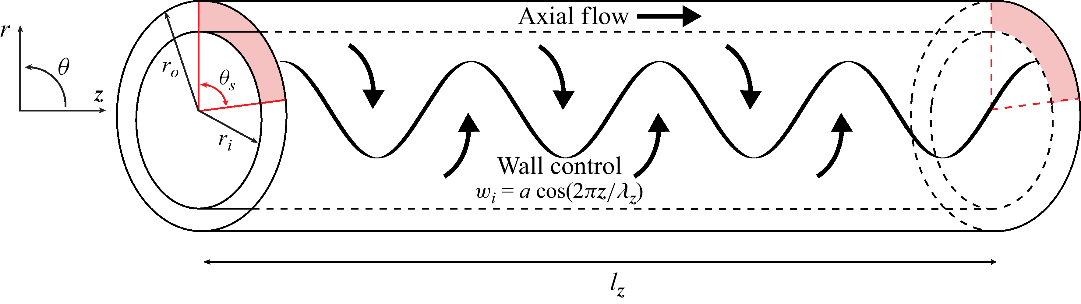
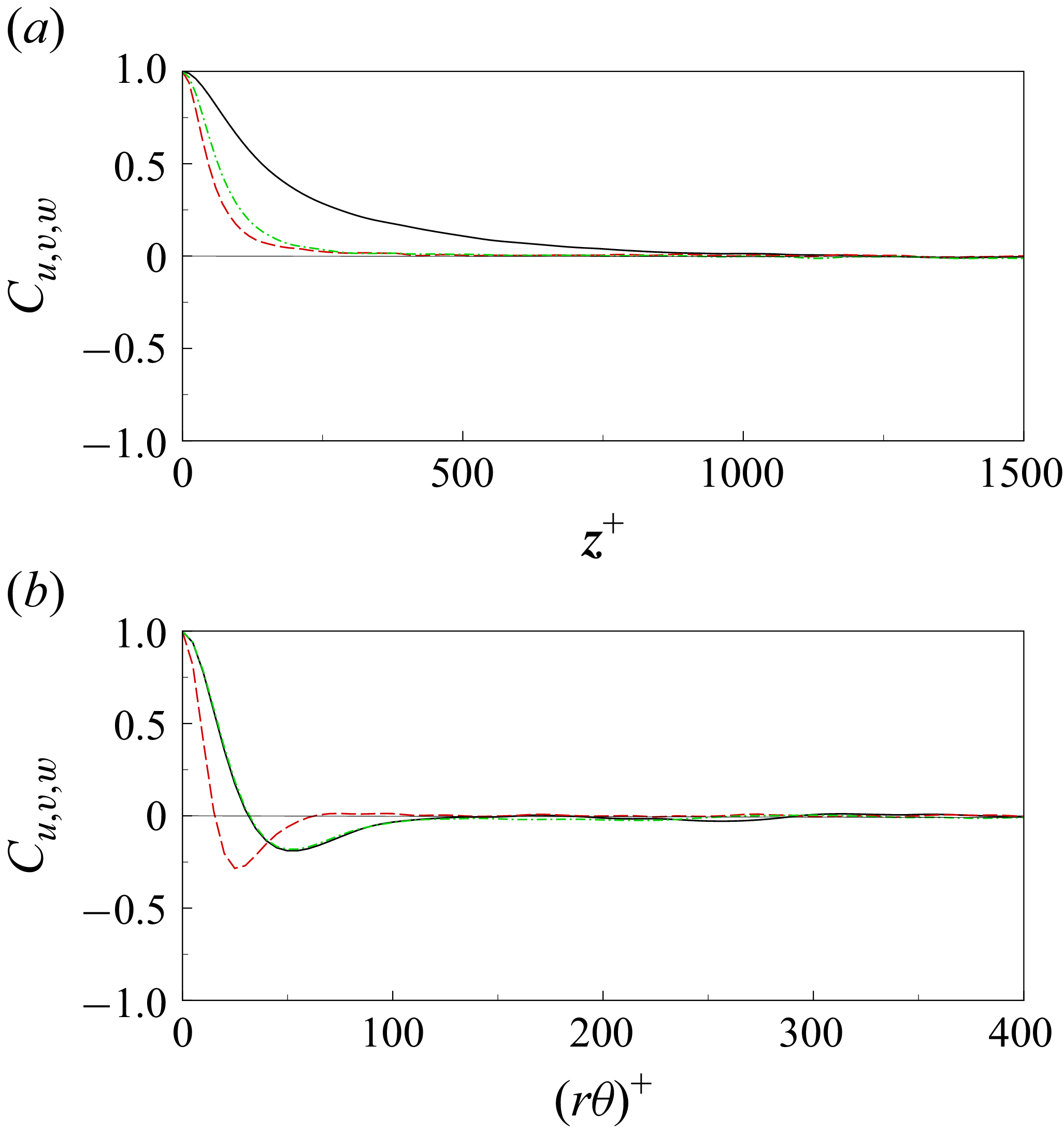
 z
 θ
 y+=5
 Cu
 Cv
 Cw
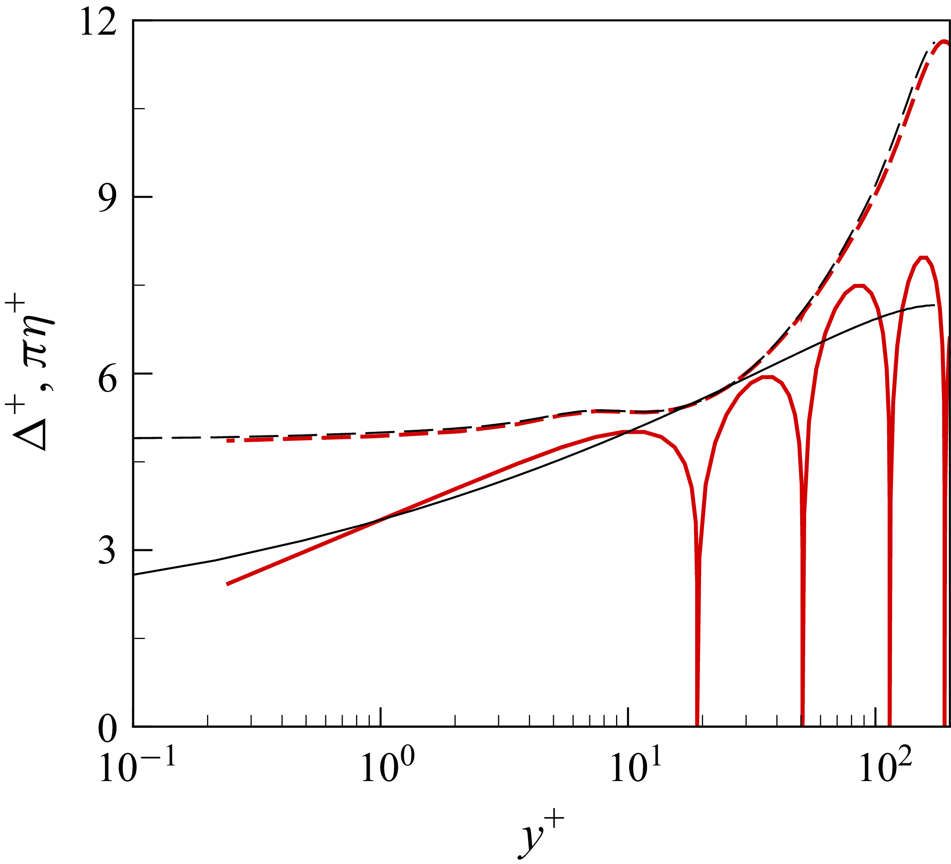
 Δ+
 πη+
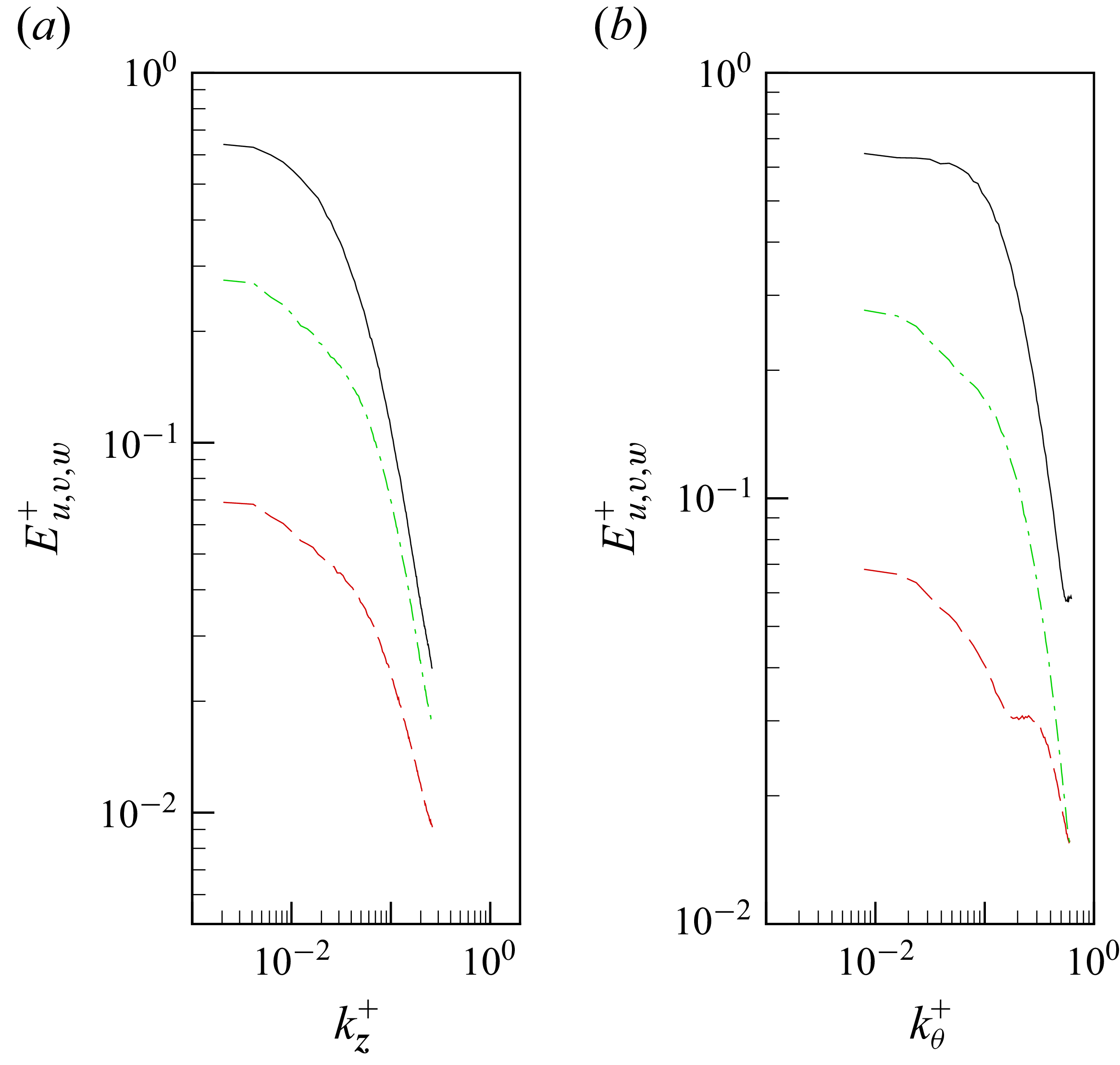
 z
 θ
 y+=5
 Eu+
 Ev+
 Ew+
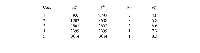
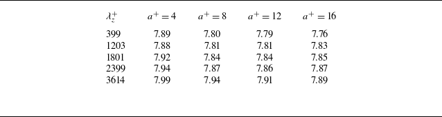
 Cf,o×103
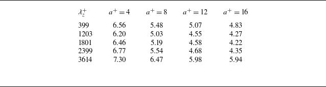
 Cf,i×103
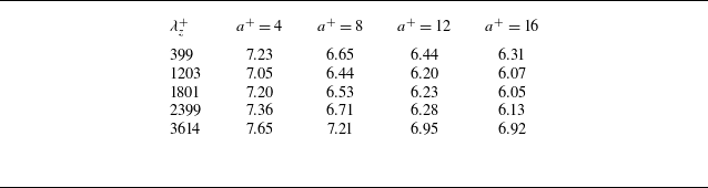
 PzS×103
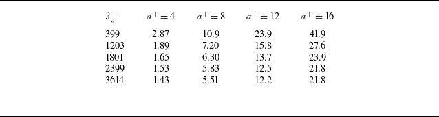
 PθS×104
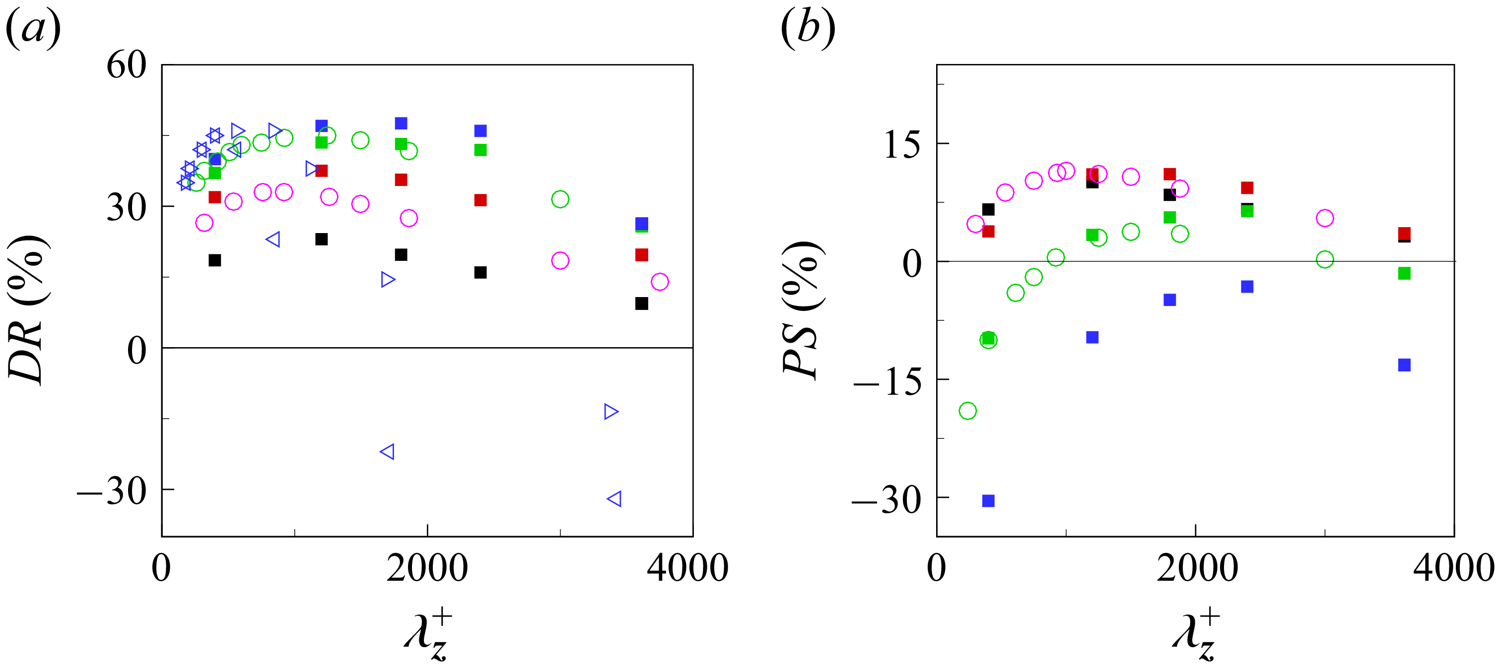
 DR
 PS
 a+=4
 a+=8
 a+=12
 a+=16
 a+=6
 a+=12
 a+=16
 η=0.25
 η=0.50
 PS

 u′
 z−θ
 y∗=5
 θ−y
 z∗=500
 z∗=2000
 a+=4
 a+=8
 a+=12
 a+=16

 u′
 z−θ
 y+=5
 θ−y
 z+=500
 z+=2000
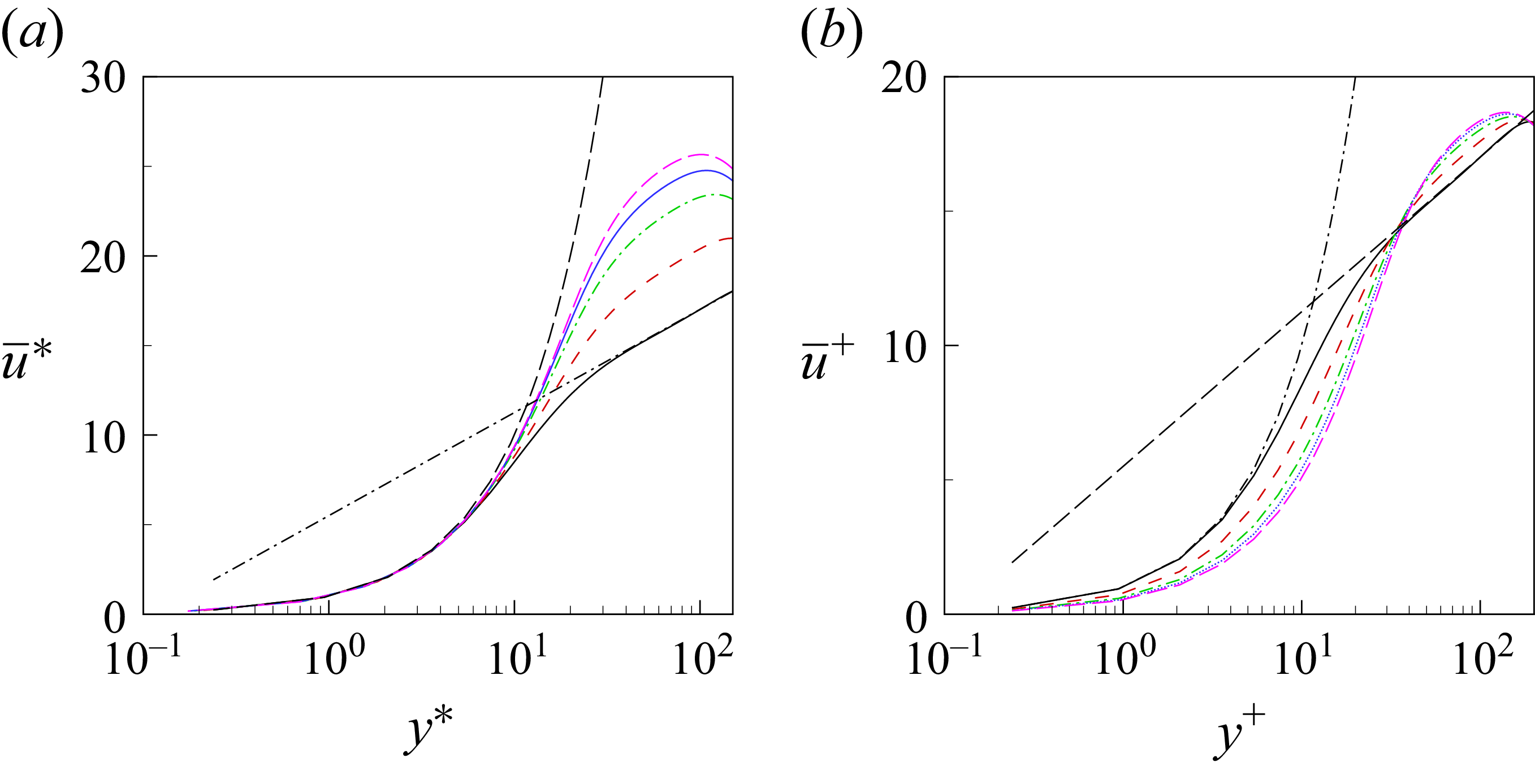
 a+=4
 a+=8
 a+=12
 a+=16
 u¯=2.5ln(y)+5.5
 u¯=y

 Ruu+=u′u′¯+
 Rvv+=v′v′¯+
 Rww+=w′w′¯+
 Ruv+=u′v′¯+
 a+=4
 a+=8
 a+=12
 a+=16
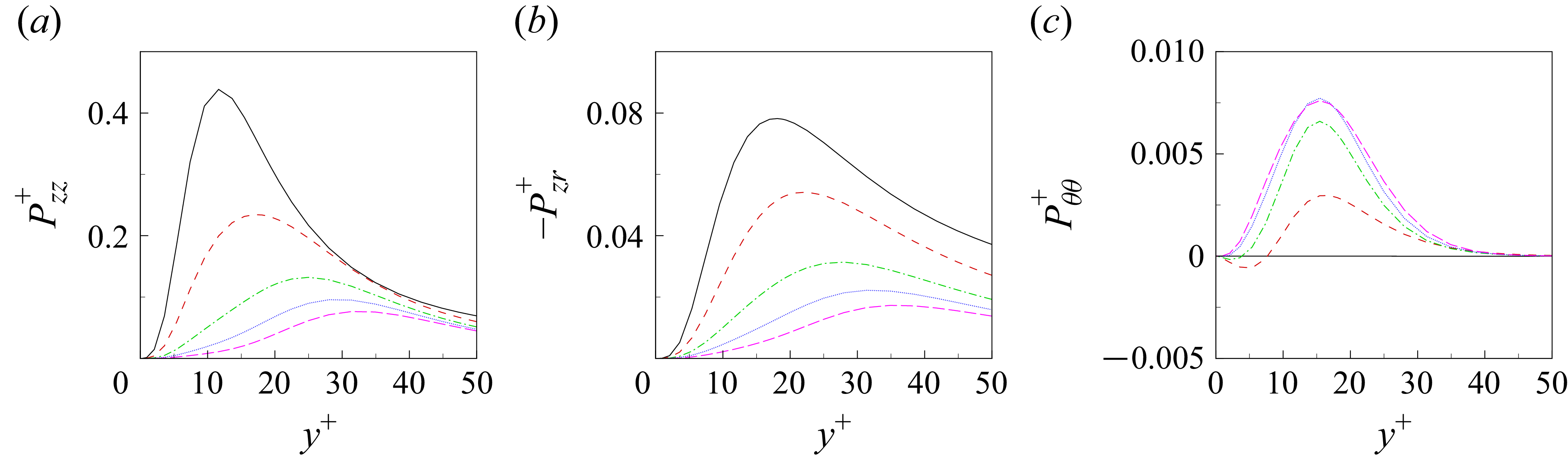
 Pzz+
 −Pzr+
 Pθθ+
 a+=4
 a+=8
 a+=12
 a+=16
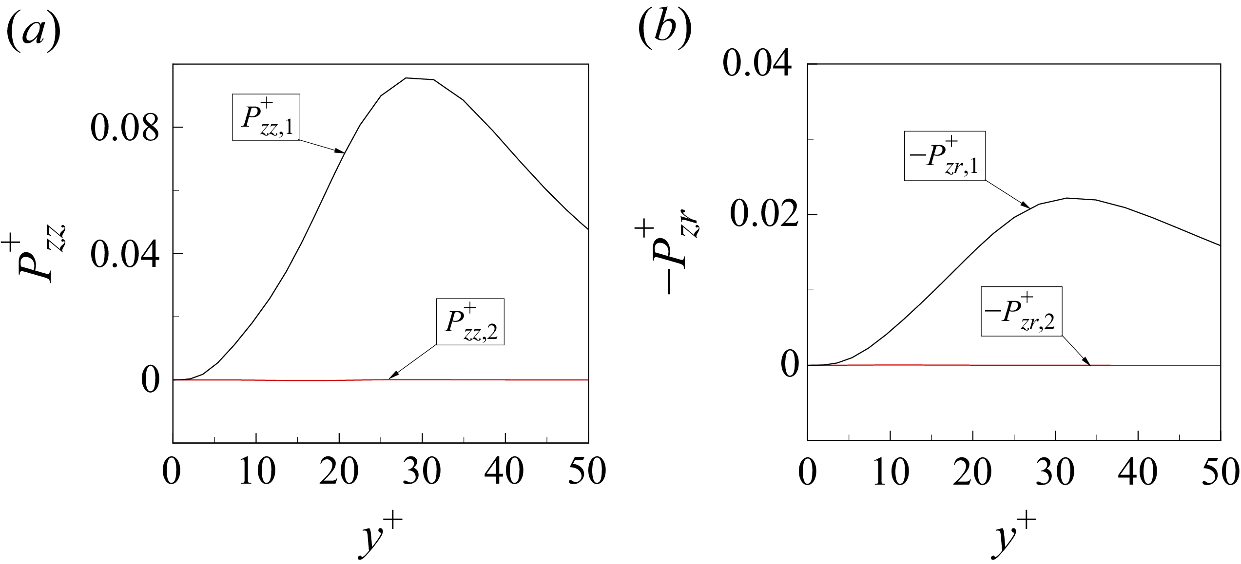
 a+=12)
 Pzz+
 −Pzr+
 Pzz,2+
 −Pzr,2+
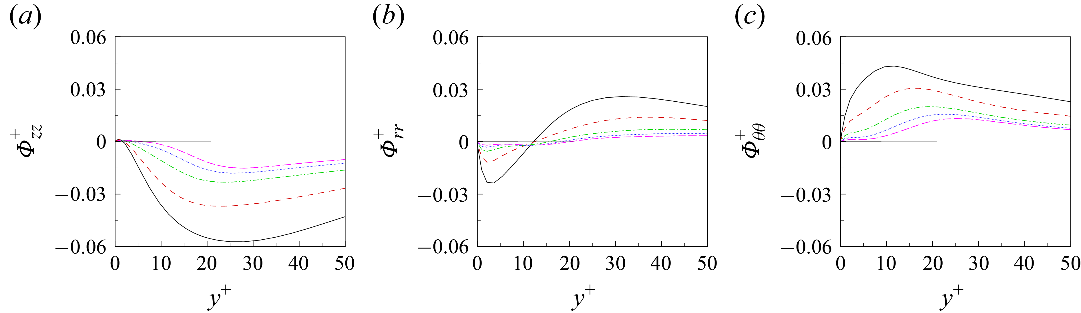
 Φzz+
 Φrr+
 Φθθ+
 a+=4
 a+=8
 a+=12
 a+=16
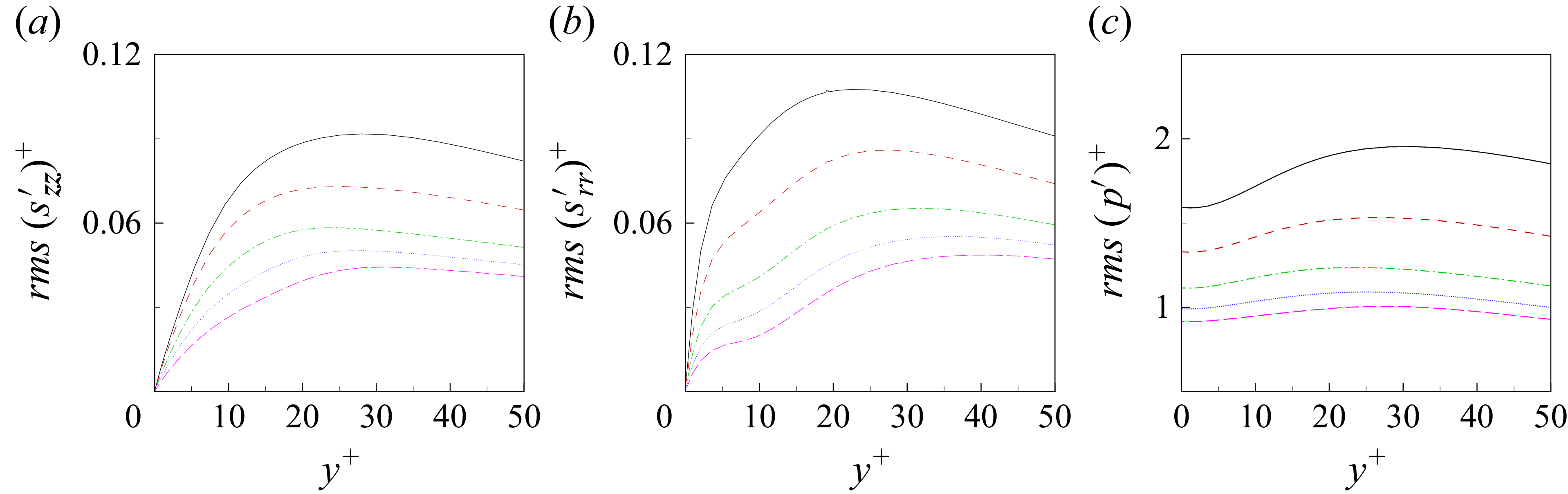
 rms(szz′)+
 rms(srr′)+
 rms(p′)+
 a+=4
 a+=8
 a+=12
 a+=16
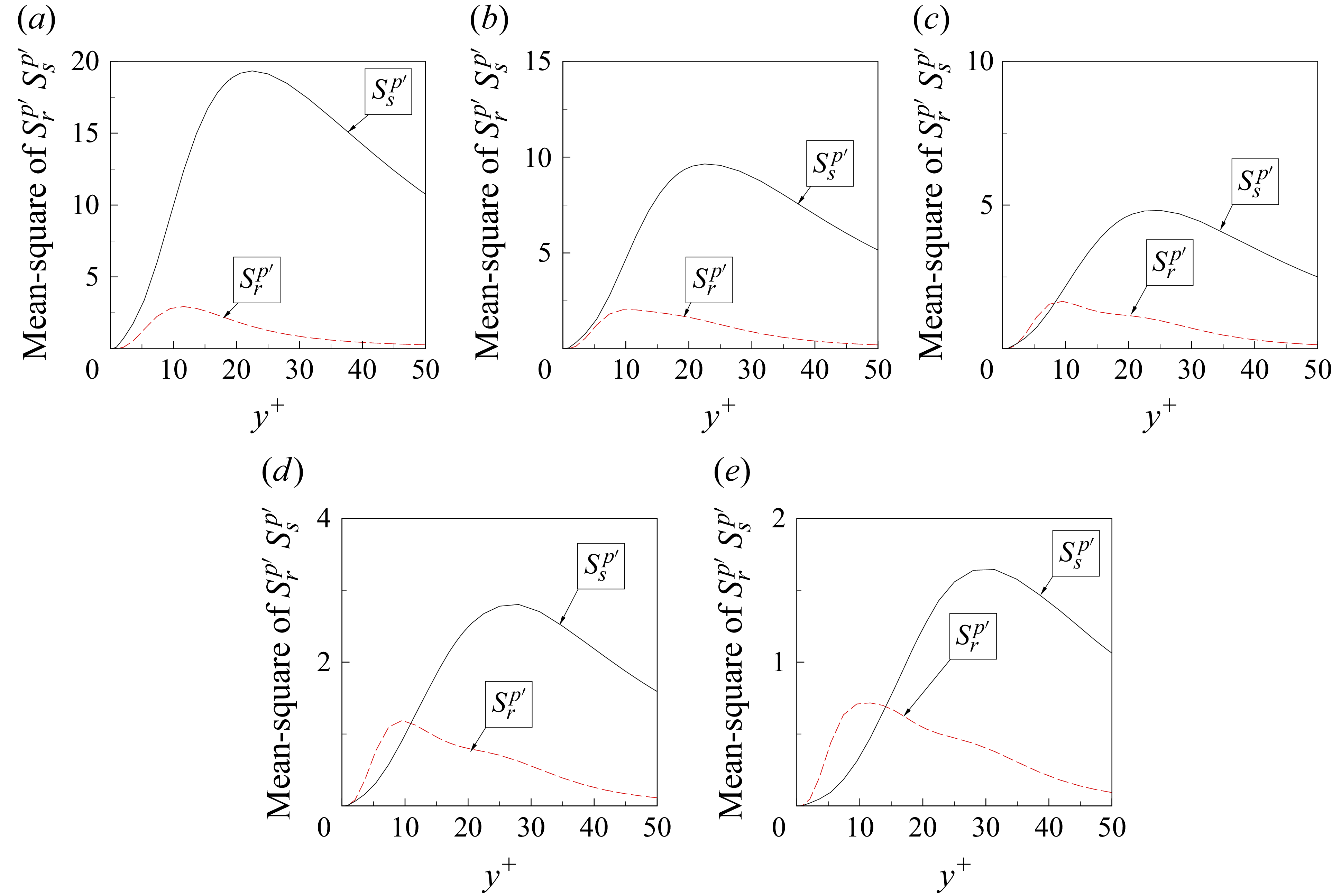
 Srp′
 Ssp′
 a+=4
 a+=8
 a+=12
 a+=16
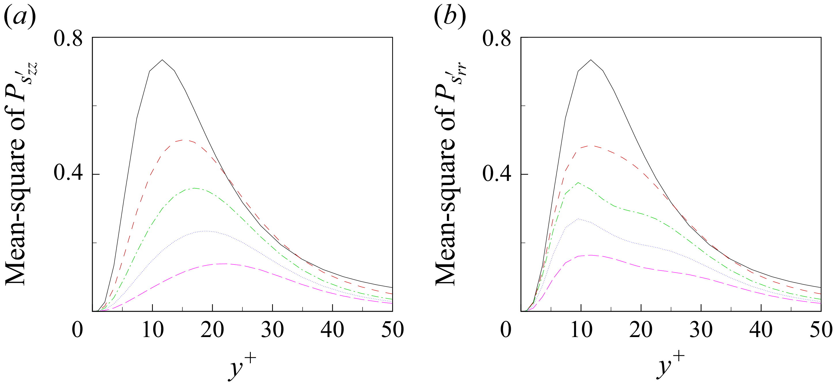
 Pszz′
 Psrr′
 a+=4
 a+=8
 a+=12
 a+=16
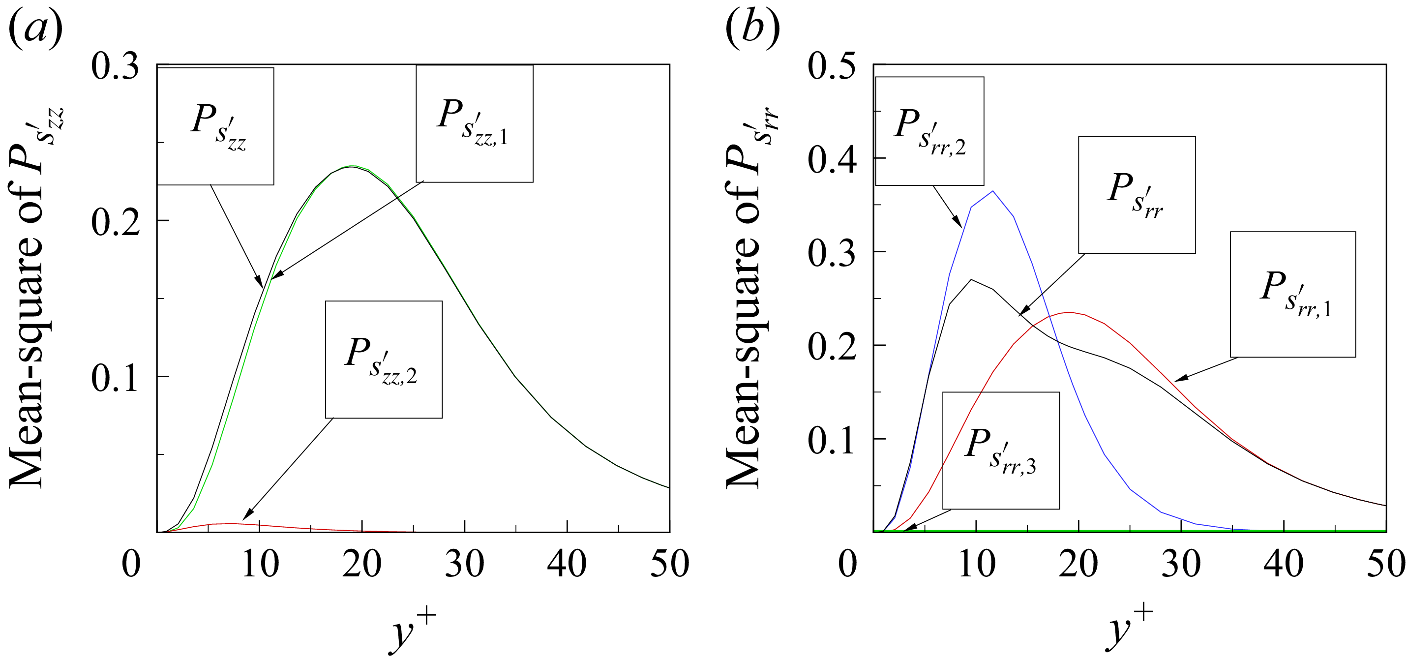
 Pszz′
 Psrr′
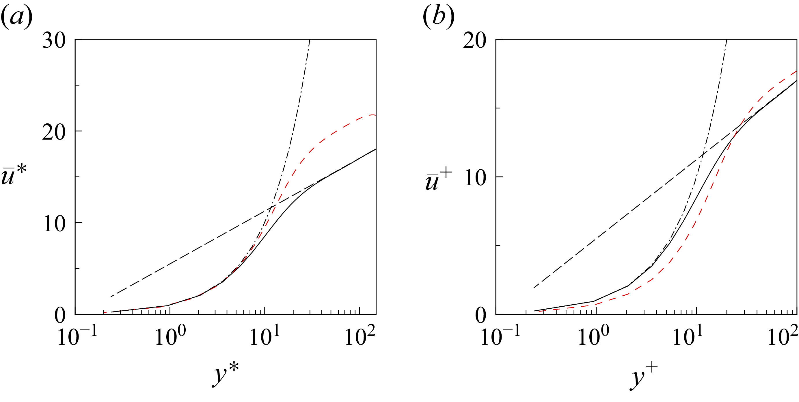
 u¯=2.5ln(y)+5.5
 u¯=y
 v′
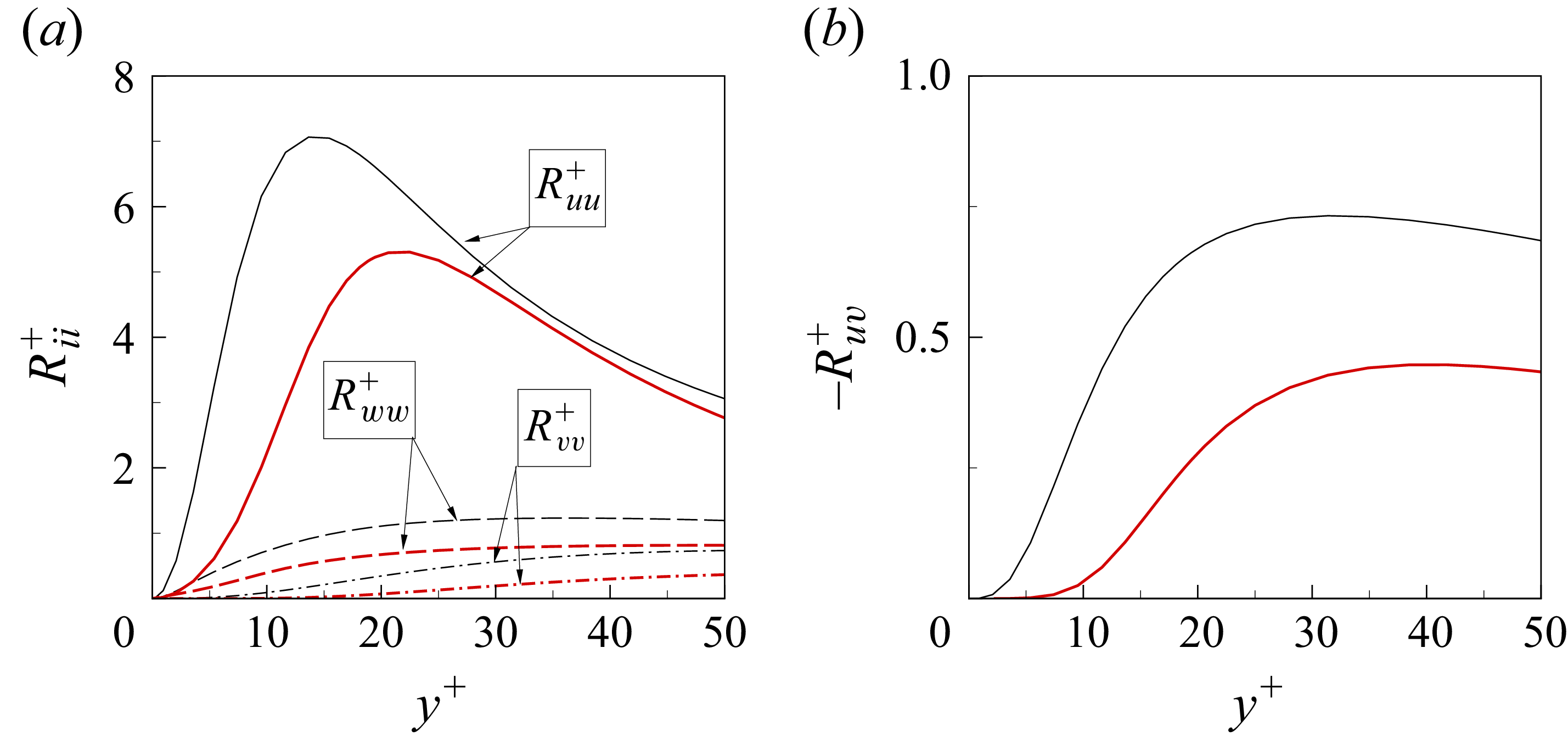
 Ruu+=u′u′¯+
 Rvv+=v′v′¯+
 Rww+=w′w′¯+
 Ruv+=u′v′¯+
 v′

 Pzz+
 Dzz+
 −ϵzz+
 Φrr+
 Ψrr+
 −ϵrr+
 Pθθ+
 Φθθ+
 Dθθ+
 −ϵθθ+
 Pzr+
 Πzr+
 Tzr+
 a+=12)

 Srp′
 Ssp′
 a+=12

 Open access

