2.1. The inner problem

We refer to the domain $\mathbb {F}$ in figure 1(a) as the microscopic domain, in opposition to the outer, macroscopic domain, formed by the fluid region far from the membrane (figure 1b). In the inner domain, we employ the following scaling:

(2.2a–d)\begin{equation} \hat{p}=\Delta \mathcal{P} p=\frac{\mu \mathcal{U}}{\ell}p, \quad \hat{u}=\mathcal{U}u, \quad \hat{\mathsf{t}}=T\mathsf{t}=\frac{\ell}{\mathcal{U}}\mathsf{t}, \quad \hat{c}=Cc, \end{equation}

where $\Delta \mathcal {P}, \mathcal {U}, T$ and $C$ are the scales of pressure difference, velocity, time and concentration at the pore level, respectively. The equations governing the physics within the microscopic elementary cell, $\mathbb {F}$, are

(2.3) \begin{equation} \left.\begin{array}{c@{}} Re_{\ell}(\partial_{\mathsf{t}}u_i+ u_j\partial_j u_i)={-}\partial_i p+ \partial_{ll}^2 u_i,\\ \partial_i u_i=0,\\ Pe_{\ell}\partial_{\mathsf{t}} c={-}Pe_{\ell} u_i \partial_i c+\partial^2_{ll} c, \end{array}\right\} \end{equation}

where $Pe_{\ell }=\mathcal {U}\ell /D$ and $Re_{\ell }=\mathcal {U}\ell /\nu$ are the Péclet and Reynolds numbers referring to the microscopic length $\ell$, respectively. The flow is assumed to be periodic along the tangential-to-the-membrane directions. No-slip ($u_i=0$) and chemostat-like ($c=0$) boundary conditions are imposed on the fluid–solid interface $\partial \mathbb {M}$. These Dirichlet boundary conditions are contained in the more general set of Robin boundary conditions presented by Zampogna et al. (Reference Zampogna, Ledda and Gallaire2022). The inner flow is assumed continuous with the outer flow, in terms of velocity, stress, concentration and solute flux at the upward $\mathbb {U}$ and downward $\mathbb {D}$ sides (cf. figure 1) of the microscopic domain.

2.2. The outer problem

In the macroscopic domain, we employ the following non-dimensionalization to scale the equations:

(2.4a–d)\begin{equation} \hat{p}=\Delta \mathcal{P}^{\mathbb{O}} p^{\mathbb{O}}=\rho {\mathcal{U}^{\mathbb{O}}}^2 p^{\mathbb{O}}, \quad \hat{u}=\mathcal{U}^{\mathbb{O}} u^{\mathbb{O}}, \quad \hat{\mathsf{t}}=T^{\mathbb{O}} \mathsf{t}^{\mathbb{O}}=\frac{L}{\mathcal{U}^{\mathbb{O}}}\mathsf{t}^{\mathbb{O}}, \quad \hat{c}=C^{\mathbb{O}}c^{\mathbb{O}}. \end{equation}

The governing equations of the outer problem are

(2.5) \begin{equation} \left.\begin{array}{c@{}} \partial_{\mathsf{t}}u_i^{\mathbb{O}}+u_j^{\mathbb{O}}\partial_j u_i^{\mathbb{O}} ={-}\partial_i p^{\mathbb{O}}+ \dfrac{1}{Re_L}\partial_{ll}^2 u^{\mathbb{O}}_i,\\ \partial_i u^{\mathbb{O}}_i=0,\\ Pe_L\partial_{\mathsf{t}} c^{\mathbb{O}}={-}Pe_L u_i^{\mathbb{O}} \partial_i c^{\mathbb{O}}+\partial^2_{ll} c^{\mathbb{O}}, \end{array}\right\} \end{equation}

where $Pe_L=\mathcal {U}^{\mathbb {O}}L/D$ and $Re_L=\mathcal {U}^{\mathbb {O}}L/\nu$.

2.3. Matching the inner and outer domains

To observe inertial effects at the pore scale, we require at least $Re_L\sim Pe_L\sim 1/\epsilon$ and $Re_{\ell }\sim Pe_{\ell }\sim 1$, and thus we assume $\mathcal {U}\sim \mathcal {U}^{\mathbb {O}}$. Consequently, the ratio of microscopic and macroscopic time scales reads

(2.6)\begin{equation} \frac{T}{T^{\mathbb{O}}}=\frac{\ell}{\mathcal{U}}\frac{\mathcal{U}^{\mathbb{O}}}{L}=\epsilon \frac{\mathcal{U}^{\mathbb{O}}}{\mathcal{U}}\sim \epsilon. \end{equation}

Equation (2.6) suggests that variations at the micro-scale occur in a much shorter time compared with the characteristic time variations at the macro-scale, and thus the pore-scale problem can be considered steady if no unsteadiness is triggered at the micro-scale,

(2.7) \begin{equation} \left.\begin{array}{c@{}} Re_{\ell} u_j\partial_j u_i={-}\partial_i p+ \partial_{ll}^2 u_i,\\ \partial_i u_i=0,\\ -Pe_{\ell} u_i \partial_i c+\partial^2_{ll} c=0. \end{array}\right\}\end{equation}

On the upward $\mathbb {U}$ and downward $\mathbb {D}$ sides of $\mathbb {F}$, the dimensional outer and inner fluid flow and concentration fields match, i.e.

(2.8a)\begin{align} \hat{\varSigma}_{ij}n_j &= \hat{\varSigma}^{\mathbb{O}}_{ij}n_j \Rightarrow [-\hat{p}\delta_{ij}+\mu(\hat{\partial}_i \hat{u}_j+\hat{\partial}_j \hat{u}_i)]n_j = [-\hat{p}^{\mathbb{O}}\delta_{ij}+\mu(\hat{\partial}_i \hat{u}^{\mathbb{O}}_j+\hat{\partial}_j \hat{u}^{\mathbb{O}}_i)]n_j\nonumber\\ &\Rightarrow\left[-\frac{\mu \mathcal{U}}{\ell}p\delta_{ij}+\frac{\mu \mathcal{U}}{\ell}(\partial_i u_j+\partial_j u_i)\right]n_j = \left[-\rho {\mathcal{U}^{\mathbb{O}}}^2 p^{\mathbb{O}}\delta_{ij}+\frac{\mu \mathcal{U}^{\mathbb{O}}}{L}(\partial_i u_j^{\mathbb{O}}+\partial_j u_i^{\mathbb{O}})\right]n_j\nonumber\\ &\Rightarrow \varSigma_{ij}n_j=\epsilon \,Re_L \frac{\mathcal{U}^{\mathbb{O}}}{ \mathcal{U}}\varSigma_{ij}^{\mathbb{O}}n_j, \end{align}

(2.8b)\begin{align} \hat{F}_i n_i&=\hat{F}_i^{\mathbb{O}} n_i\Rightarrow [ \hat{u}_i\hat{c}-D\hat{\partial}_i \hat{c} ]n_i=[ \hat{u}^{\mathbb{O}}_i\hat{c}^{\mathbb{O}}-D\hat{\partial}_i \hat{c}^{\mathbb{O}} ]n_i \nonumber\\ &\Rightarrow\left[ \mathcal{U}C u_i c-D\frac{C}{\ell}\partial_i c \right]n_i=\left[ \mathcal{U}^{\mathbb{O}}C^{\mathbb{O}} u_i^{\mathbb{O}} c^{\mathbb{O}}-D\frac{C^{\mathbb{O}}}{L}\partial_i c^{\mathbb{O}} \right]n_i\nonumber\\ &\Rightarrow F_in_i=\epsilon\frac{C^{\mathbb{O}}}{C}F_i^{\mathbb{O}}n_i, \end{align}

(2.8c,d)\begin{align} u&=\frac{\mathcal{U}^{\mathbb{O}}}{\mathcal{U}}u^{\mathbb{O}}, \quad c=\frac{C^{\mathbb{O}}}{C}c^{\mathbb{O}}, \end{align}

where $\varSigma _{jk}=-p\delta _{jk}+(\partial _j u_k+\partial _k u_j)$, $\varSigma _{jk}^{\mathbb {O}}=-p^{\mathbb {O}}\delta _{jk}+\frac {1}{Re_L}(\partial _j u^{\mathbb {O}}_k+\partial _k u^{\mathbb {O}}_j)$, $F_j=Pe_{\ell } u_i c - \partial _i c$ and $F_j^{\mathbb {O}}=Pe_L u_i^{\mathbb {O}} c^{\mathbb {O}} - \partial _i c^{\mathbb {O}}$ are the fluid stresses and solute fluxes in the inner and outer domains, respectively.

2.4. Solving the inner problem

To apply homogenization to the problem in (2.7), the Stokes approximation assumes $Re_{\ell }\sim Pe_{\ell }\sim \epsilon$ (Zampogna et al. Reference Zampogna, Ledda and Gallaire2022). In this paper, we introduce finite Péclet and Reynolds numbers at the pore scale, i.e. $Re_{\ell }\sim 1$ and $Pe_{\ell }\sim 1$. Consequently, the problem in (2.7) is a set of nonlinear partial differential equations. Exploiting the separation of scales, we perform the following asymptotic expansion:

(2.9) \begin{equation} \left.\begin{array}{c@{}} x_i=x_i+\epsilon X_i, \quad \partial_i =\partial_i+\epsilon \partial_I, \\ (u_i,p,c)=(u_i^{(0)},p^{(0)},c^{(0)})+\epsilon (u_i^{(1)},p^{(1)},c^{(1)})+\mathcal{O}(\epsilon^2). \end{array}\right\} \end{equation}

Substituting (2.9) into (2.7), we obtain the leading order equation,

(2.10) \begin{equation} \left.\begin{array}{c@{}} Re_{\ell} u_j^{(0)}\partial_j u_i^{(0)}={-}\partial_i p^{(0)}+ \partial_{ll}^2 u_i^{(0)},\\ \partial_i u_i^{(0)}=0,\\ -Pe_{\ell} u_i^{(0)} \partial_i c^{(0)}+\partial^2_{ll} c^{(0)}=0,\\ \varSigma_{ij}^{(0)}n_j=\varSigma_{ij}^{\mathbb{O}}n_j \quad \text{on } \mathbb{U},\mathbb{D},\\ u_i^{(0)}=0 \quad \text{on } \partial\mathbb{M},\\ u_i^{(0)},p^{(0)} \quad \text{periodic along } \boldsymbol{t},\boldsymbol{s}. \end{array}\right\} \end{equation}

To write the solution of (2.10) as a linear combination of the boundary fluxes, we introduce the closure advective velocity $U_j$ such that

(2.11) \begin{equation} \left.\begin{array}{c@{}} Re_{\ell} U_j\partial_j u_i^{(0)}={-}\partial_i p^{(0)}+ \partial_{ll}^2 u_i^{(0)},\\ \partial_i u_i^{(0)}=0,\\ -Pe_{\ell} U_j \partial_j c^{(0)}+\partial^2_{ll} c^{(0)}=0,\\ \varSigma_{ij}^{(0)}n_j=\varSigma_{ij}^{\mathbb{O}}n_j \quad \text{on } \mathbb{U},\mathbb{D},\\ u_i^{(0)}=0 \quad \text{on } \partial\mathbb{M},\\ u_i^{(0)},p^{(0)} \quad \text{periodic along } \boldsymbol{t},\boldsymbol{s}. \end{array}\right\}\end{equation}

The term $U_j$ needs to be specified to close (2.11). However, we refer to § 2.6 for the closure of $U_j$. The solution of (2.11) can be formally written as a linear combination of the boundary fluxes,

(2.12) \begin{equation} \left.\begin{array}{c@{}} u_i^{(0)}=\epsilon Re_L \dfrac{\mathcal{U}^{\mathbb{O}}}{\mathcal{U}}(M_{ij}\varSigma_{jk}^{\mathbb{O,U}}n_k+N_{ij}\varSigma_{jk}^{\mathbb{O,D}}n_k),\\ p^{(0)}=\epsilon Re_L \dfrac{\mathcal{U}^{\mathbb{O}}}{\mathcal{U}}(Q_{j}\varSigma_{jk}^{\mathbb{O,U}}n_k+R_{j}\varSigma_{jk}^{\mathbb{O,D}}n_k),\\ c^{(0)}=\epsilon \dfrac{C^{\mathcal{O}}}{C} (T F_j^{\mathbb{O,U}}n_j+S F_j^{\mathbb{O,D}}n_j). \end{array}\right\}\end{equation}

Substituting (2.12) into (2.11), we obtain the set of solvability conditions:

(2.13a) \begin{gather} \left.\begin{array}{c@{}} Re_{\ell} U_m \partial_m M_{ij}={-}\partial_i Q_{j} +\partial^2_{ll}M_{ij} \quad \text{in } \mathbb{F},\\ \partial_i M_{ij}=0 \quad \text{in } \mathbb{F},\\ \varSigma_{pq}(M_{\cdot j},Q_{j})n_q=\delta_{jp}n_q \quad \text{on } \mathbb{U},\\ \varSigma_{pq}(M_{\cdot j},Q_{j})n_q=0 \quad \text{on } \mathbb{D},\\ M_{ij}=0 \quad \text{on } \partial \mathbb{M},\\ M_{ij},Q_{j} \quad \text{periodic along } \boldsymbol{t},\boldsymbol{s}, \end{array}\right\} \end{gather}

(2.13b) \begin{gather} \left.\begin{array}{c@{}} Re_{\ell} U_m \partial_m N_{ij}={-}\partial_i R_{j} +\partial^2_{ll}N_{ij} \quad \text{in } \mathbb{F},\\ \partial_i N_{ij}=0 \quad \text{in } \mathbb{F},\\ \varSigma_{pq}(N_{\cdot j},R_{j})n_q=0 \quad \text{on } \mathbb{U},\\ \varSigma_{pq}(N_{\cdot j},R_{j})n_q=\delta_{jp}n_q \quad \text{on } \mathbb{D},\\ N_{ij}=0 \quad \text{on } \partial \mathbb{M},\\ N_{ij},R_{j} \quad \text{periodic along } \boldsymbol{t},\boldsymbol{s}, \end{array}\right\} \end{gather}

(2.13c,d) \begin{gather} \left.\begin{array}{c@{}} Pe_{\ell} U_j \partial_j T-\partial^2_{ll}T = 0 \quad \text{in } \mathbb{F}, \\ (Pe_{\ell} U_j T-\partial_jT)n_j = 1 \quad \text{on } \mathbb{U},\\ (Pe_{\ell} U_j T-\partial_jT)n_j = 0 \quad \text{on } \mathbb{D},\\ T = 0 \quad \text{on } \partial\mathbb{M}, \\ T \quad \text{periodic along } \boldsymbol{t},\boldsymbol{s}, \end{array}\right\}\quad \left.\begin{array}{c@{}} Pe_{\ell} U_j \partial_j S-\partial^2_{ll} S = 0 \quad \text{in } \mathbb{F},\\ (Pe_{\ell} U_j S-\partial_j S)n_j = 0 \quad \text{on } \mathbb{U}, \\ (Pe_{\ell} U_j S-\partial_j S)n_j = 1 \quad \text{on } \mathbb{D}, \\ S = 0 \quad \text{on } \partial\mathbb{M}, \\ S \quad \text{periodic along } \boldsymbol{t},\boldsymbol{s}, \end{array}\right\} \end{gather}

where $\varSigma _{pq}(M_{\cdot j},Q_j)=-Q_j\delta _{pq}+(\partial _q M_{pj} + \partial _p M_{qj})$ and similarly for $N_{ij},R_j$. Since $\varSigma _{pq}$ contain the quantities $Q_j, R_j$, no additional boundary condition is needed for the closing of these equations. The first (second) problem in (2.13) represents the pore-level solvent transport in response to normal and tangential unitary stresses on the upward side $\mathbb {U}$ (downward side $\mathbb {D}$) of the membrane. Conversely, the third (fourth) problem represents the pore-level solute transport across the membrane caused by a unitary solute flux entering the upward side $\mathbb {U}$ (downward side $\mathbb {D}$) of the membrane. We notice that by integrating in $\mathbb {F}$ the last two problems in (2.13) and applying the divergence theorem, we obtain an integral balance of solute fluxes which states that the solute flux entering from the $\mathbb {U}$ or $\mathbb {D}$ side is removed from the domain at the boundary $\partial \mathbb {M}$ because of its boundary condition. The solvability conditions in (2.13) slightly differ from those introduced by Zampogna et al. (Reference Zampogna, Ledda and Gallaire2022) because of the presence of the advective term. In the case of flows on rough, impermeable surfaces, Bottaro (Reference Bottaro2019) and Lācis et al. (Reference Lācis, Sudhakar, Pasche and Bagheri2020) showed that the systems in (2.13) are equivalent to the following set of equations:

(2.14a) $$\begin{gather} \left.\begin{array}{c@{}} Re_{\ell} U_m \partial_m M_{ij}={-}\partial_i Q_{j} +\partial^2_{ll}M_{ij} +\delta_{\mathbb{C}}\delta_{ij},\\ \partial_i M_{ij}=0,\\ \varSigma_{pq}(M_{\cdot j},Q_{j})n_q=0 \quad \text{on } \mathbb{U}, \mathbb{D},\\ M_{ij}=0 \quad \text{on } \partial \mathbb{M},\\ M_{ij},Q_{j} \quad \text{periodic along } \boldsymbol{t},\boldsymbol{s}, \end{array}\right\} \end{gather}$$

(2.14b) $$\begin{gather}\left.\begin{array}{c@{}} Re_{\ell} U_m \partial_m N_{ij}={-}\partial_i R_{j} +\partial^2_{ll}N_{ij}-\delta_{\mathbb{C}}\delta_{ij},\\ \partial_i N_{ij}=0,\\ \varSigma_{pq}(N_{\cdot j},R_{j})n_q=0 \quad \text{on } \mathbb{U}, \mathbb{D},\\ N_{ij}=0 \quad \text{on } \partial \mathbb{M},\\ N_{ij},R_{j} \quad \text{periodic along } \boldsymbol{t},\boldsymbol{s}, \end{array}\right\} \end{gather}$$

(2.14c) $$\begin{gather}\left.\begin{array}{c@{}} Pe_{\ell} U_j \partial_j T-\partial^2_{ll}T+\delta_{\mathbb{C}} = 0 \quad \text{in } \mathbb{F}, \\ (Pe_{\ell} U_j T-\partial_jT)n_j = 0 \quad \text{on } \mathbb{U}, \mathbb{D},\\ T = 0 \quad \text{on } \partial\mathbb{M}, \\ T \quad \text{periodic along } \boldsymbol{t},\boldsymbol{s}, \end{array}\right\} \end{gather}$$

(2.14d) $$\begin{gather}\left.\begin{array}{c@{}} Pe_{\ell} U_j \partial_j S-\partial^2_{ll} S-\delta_{\mathbb{C}} = 0 \quad \text{in } \mathbb{F},\\ (Pe_{\ell} U_j S-\partial_j S)n_j = 0 \quad \text{ on } \mathbb{U}, \mathbb{D}, \\ S = 0 \quad \text{ on } \partial\mathbb{M}, \\ S \quad \text{periodic along } \boldsymbol{t},\boldsymbol{s}, \end{array}\right\} \end{gather}$$

where $\delta _{\mathbb {C}}$ is a Dirac impulse centred in $x_{\mathbb {C}}$. The physical significance of the problems in (2.13) and (2.14) is similar, but here the forcing is represented by a unitary volume source appearing in the momentum and advection–diffusion equations. The quantities $M_{ij},N_{ij},Q_i,R_i,T$ and $S$ depend parametrically on the closure advective velocity $U_j$. In the present paper, we adopt the formulation in (2.14) to compute the microscopic solution.

2.5. Averaging step and macroscopic condition

To upscale the microscopic solutions, we introduce the following averages at both the upstream and downstream sides of the membrane:

(2.15a,b)\begin{equation} \bar{M}_{ij}=\frac{1}{|\mathbb{U}|}\int_{\mathbb{U}} M_{ij} \,{\rm d}\kern 0.06em x_t \,{\rm d}\kern 0.06em x_s, \quad \bar{N}_{ij}=\frac{1} {|\mathbb{D}|}\int_{\mathbb{D}} N_{ij} \,{\rm d}\kern 0.06em x_t \,{\rm d}\kern 0.06em x_s. \end{equation}

We clarify the physical significance of the $\bar {M}_{ij}$ tensors in a two-dimensional domain: $\bar {M}_{nn}$ and $\bar {M}_{tn}$ represent the ability of the fluid to move along the positive normal and tangential directions as a consequence of a normal unitary forcing. Instead, $\bar {M}_{nt}$ and $\bar {M}_{tt}$ represent the ability of the fluid to move along the positive normal and tangential directions as a consequence of a tangential unitary forcing. The same applies for $\bar {N}_{ij}$, with negative normal and tangential directions. Thus, $\bar {M}_{nn}$ and $\bar {M}_{tt}$ can be interpreted as a permeability and a slip coefficient, respectively. The same average definitions apply to the quantities $T$ and $S$,

(2.16a,b)\begin{equation} \bar{T}=\frac{1}{|\mathbb{U}|}\int_{\mathbb{U}} T \,{\rm d}\kern 0.06em x_t \,{\rm d}\kern 0.06em x_s, \quad \bar{S}=\frac{1} {|\mathbb{D}|}\int_{\mathbb{D}} S \,{\rm d}\kern 0.06em x_t \,{\rm d}\kern 0.06em x_s. \end{equation}

These quantities can be interpreted as effective solute diffusivities relative to a unitary solute flux in the positive ($\bar {T}$) and negative ($\bar {S}$) directions. Quantities $\boldsymbol {M},\boldsymbol {N}, T, S$ are not solely properties of the geometry (as in the inertia-less case of Zampogna & Gallaire Reference Zampogna and Gallaire2020), but also of the fluid flow since they depend on the closure advective velocity.

Applying averages ((2.15), (2.16)) to (2.12), the following macroscopic boundary conditions are obtained:

(2.17) \begin{equation} \left.\begin{array}{c@{}} \bar{u}_i^{\mathbb{O}}=\epsilon Re_L(\bar{M}_{ij}\varSigma_{jk}^{\mathbb{O,U}}n_k+\bar{N}_{ij}\varSigma_{jk}^{\mathbb{O,D}}n_k),\\ \bar{c}^{\mathbb{O}}=\epsilon (\bar{T} F_j^{\mathbb{O,U}}n_j+\bar{S} F_j^{\mathbb{O,D}}n_j). \end{array}\right\} \end{equation}

We specify that (2.17) is obtained from (2.12) by re-normalizing with the outer scales in (2.8).

2.6. The closure advective velocity

The solution to (2.14) lies in the closure advective velocity that gives rise to an inertia-driven coupling between the macroscopic and microscopic flows. Two different definitions have been considered in the present work:

1. (i) a constant advective velocity in the microscopic cell

   (2.18)\begin{equation} U_i=\bar{u}_i^{\mathbb{O}}, \end{equation}
   which leads to an Oseen-like equation (constant advection closure). This approach has already been proposed in the volume-averaged and homogenization frameworks by other authors for the flow over rough surfaces (Bottaro Reference Bottaro2019; Zampogna, Magnaudet & Bottaro Reference Zampogna, Magnaudet and Bottaro2019);

2. (ii) a spatially dependent closure advective velocity, reconstructed from the outer stresses (variable advection closure),

   (2.19)\begin{equation} U_i=\epsilon Re_L ( M_{ij}\varSigma_{jk}^{\mathbb{O,U}}n_k+N_{ij}\varSigma_{jk}^{\mathbb{O,D}}n_k). \end{equation}
   A similar approach has been proposed for the flow in bulk porous media (Valdés-Parada & Lasseux Reference Valdés-Parada and Lasseux2021; Sánchez-Vargas et al. Reference Sánchez-Vargas, Valdés-Parada, Trujillo-Roldán and Lasseux2023).

The equations for $M_{ij}, Q_j, T$ in the microscopic problems thus become:

1. (i) for the constant advection closure approach in (2.18):

   (2.20a) $$\begin{gather} \left.\begin{array}{c@{}} \epsilon Re_L \dfrac{\mathcal{U}}{\mathcal{U}^{\mathbb{O}}}\bar{u}_m^{\mathbb{O}} \partial_m M_{ij}={-}\partial_i Q_{j} +\partial^2_{ll}M_{ij} +\delta_{\mathbb{C}}\delta_{ij},\\ \partial_i M_{ij}=0,\\ \varSigma_{pq}(M_{\cdot j},Q_{j})n_q=0 \quad \text{on } \mathbb{U}, \mathbb{D},\\ M_{ij}=0 \quad \text{on } \partial \mathbb{M},\\ M_{ij},Q_{j} \quad \text{periodic along } \boldsymbol{t},\boldsymbol{s}; \end{array}\right\} \end{gather}$$
   (2.20b) $$\begin{gather}\left.\begin{array}{c@{}} \epsilon Re_L \dfrac{\mathcal{U}}{\mathcal{U}^{\mathbb{O}}}\bar{u}_m^{\mathbb{O}} \partial_m N_{ij}={-}\partial_i R_{j} +\partial^2_{ll}N_{ij} -\delta_{\mathbb{C}}\delta_{ij},\\ \partial_i N_{ij}=0,\\ \varSigma_{pq}(N_{\cdot j},R_{j})n_q=0 \quad \text{on } \mathbb{U}, \mathbb{D},\\ N_{ij}=0 \quad \text{on } \partial \mathbb{M},\\ N_{ij},R_{j} \quad \text{periodic along } \boldsymbol{t},\boldsymbol{s}; \end{array}\right\} \end{gather}$$
   (2.20c) $$\begin{gather}\left.\begin{array}{c@{}} \epsilon Pe_L \dfrac{\mathcal{U}}{\mathcal{U}^{\mathbb{O}}}\bar{u}_i^{\mathbb{O}} \partial_j T-\partial^2 _{ll}T+\delta_{\mathbb{C}} = 0,\\ (\epsilon Pe_L \bar{u}_i^{\mathbb{O}} T-\partial_jT)n_j = 0 \quad \text{on } \mathbb{U}, \mathbb{D},\\ T = 0 \quad \text{on } \partial\mathbb{M}, \\ T \quad \text{periodic along } \boldsymbol{t},\boldsymbol{s}; \end{array}\right\} \end{gather}$$
   (2.20d) $$\begin{gather}\left.\begin{array}{c@{}} \epsilon Pe_L \dfrac{\mathcal{U}}{\mathcal{U}^{\mathbb{O}}}\bar{u}_i^{\mathbb{O}} \partial_j S-\partial^2 _{ll}S-\delta_{\mathbb{C}} = 0,\\ (\epsilon Pe_L \bar{u}_i^{\mathbb{O}} S-\partial_j S)n_j = 0 \quad \text{on } \mathbb{U}, \mathbb{D}, \\ S = 0 \quad \text{on } \partial\mathbb{M}, \\ S \quad \text{periodic along } \boldsymbol{t},\boldsymbol{s}; \end{array}\right\} \end{gather}$$

2. (ii) for the variable advection closure approach in (2.19):

   (2.21a) \begin{gather} \left.\begin{array}{c@{}} \epsilon^2 Re_L^2 \dfrac{\mathcal{U}}{\mathcal{U}^{\mathbb{O}}}(M_{mn}\varSigma_{nl}^{\mathbb{O,U}}n_l+N_{mn}\varSigma_{nl}^{\mathbb{O,D}}n_l) \partial_m M_{ij}={-}\partial_i Q_{j} +\partial^2_{ll}M_{ij} +\delta_{\mathbb{C}}\delta_{ij},\\ \partial_i M_{ij}=0,\\ \varSigma_{pq}(M_{\cdot j},Q_{j})n_q=0 \quad \text{on } \mathbb{U}, \mathbb{D},\\ M_{ij}=0 \quad \text{on } \partial \mathbb{M},\\ M_{ij},Q_{jk} \quad \text{periodic along } \boldsymbol{t},\boldsymbol{s}; \end{array}\right\} \end{gather}
   (2.21b) \begin{gather} \left.\begin{array}{c@{}} \epsilon^2 Re_L^2 \dfrac{\mathcal{U}}{\mathcal{U}^{\mathbb{O}}}(M_{mn}\varSigma_{nl}^{\mathbb{O,U}}n_l+N_{mn}\varSigma_{nl}^{\mathbb{O,D}}n_l) \partial_m N_{ij}={-}\partial_i R_{j} +\partial^2_{ll}N_{ij} -\delta_{\mathbb{C}}\delta_{ij},\\ \partial_i N_{ij}=0,\\ \varSigma_{pq}(N_{\cdot j},R_{j})n_q=0 \quad \text{on } \mathbb{U}, \mathbb{D},\\ N_{ij}=0 \quad \text{on } \partial \mathbb{M},\\ N_{ij},R_{j} \quad \text{periodic along } \boldsymbol{t},\boldsymbol{s}; \end{array}\right\} \end{gather}
   (2.21c) \begin{gather} \left.\begin{array}{c@{}} \epsilon^2 Pe_L \dfrac{\mathcal{U}}{\mathcal{U}^{\mathbb{O}}}(M_{mn}\varSigma_{nl}^{\mathbb{O,U}}n_l+N_{mn}\varSigma_{nl}^{\mathbb{O,D}}n_l) \partial_j T-\partial^2_{ll} T+\delta_{\mathbb{C}} = 0,\\ (\epsilon^2 Pe_L (M_{mn}\varSigma_{nl}^{\mathbb{O,U}}n_l+N_{mn}\varSigma_{nl}^{\mathbb{O,D}}n_l) T-\partial_jT)n_j = 0 \quad \text{on } \mathbb{U}, \mathbb{D},\\ T = 0 \quad \text{on } \partial\mathbb{M}, \\ T \quad \text{periodic along } \boldsymbol{t},\boldsymbol{s}; \end{array}\right\} \end{gather}
   (2.21d) \begin{gather} \left.\begin{array}{c@{}} \epsilon^2 Pe_L \dfrac{\mathcal{U}}{\mathcal{U}^{\mathbb{O}}}(M_{mn}\varSigma_{nl}^{\mathbb{O,U}}n_l+N_{mn}\varSigma_{nl}^{\mathbb{O,D}}n_l) \partial_j S-\partial^2_{ll} S-\delta_{\mathbb{C}} = 0,\\ (\epsilon^2 Pe_L (M_{mn}\varSigma_{nl}^{\mathbb{O,U}}n_l+N_{mn}\varSigma_{nl}^{\mathbb{O,D}}n_l) S-\partial_j S)n_j = 0 \quad \text{on } \mathbb{U}, \mathbb{D},\\ S = 0 \quad \text{on } \partial\mathbb{M}, \\ S \quad \text{periodic along } \boldsymbol{t},\boldsymbol{s}. \end{array}\right\} \end{gather}

The tensors and scalars used in (2.17) are found either by solving (2.20) or (2.21). A computational iterative strategy to interface the macroscopic fields with the microscopic problems is required.

3.1. Constant advection closure

In the constant advection closure problem, we specify the advective velocity in (2.14) as a constant field (2.18), obtaining (2.20). The solutions for the couples $(M_{nn},M_{tn}),(M_{nt},M_{tt})$ are presented in figure 3. To compact the notation, we introduce $\check {u}_i=\epsilon Re_L ({\mathcal {U}}/{\mathcal {U}^{\mathbb {O}}})\bar {u}_i^{\mathbb {O}}$ in the term in front of the convective term on the left-hand side of (2.20), the inertia-driven coupling term with the macroscopic problem. We consider three values of $\check {u}_i$, corresponding to the pure diffusive case ($\check {u}_i=0$; panels $b,e$), a case of pure normal advection ($\check {u}_n\neq 0$ and $\check {u}_t=0$; panels $c,f$), and a case of normal and tangential advection ($\check {u}_n\neq 0$, $\check {u}_t\neq 0$; panels $d,g$). Recirculating zones propagate downstream the inclusion in the direction of the advective flow. Note that the same microscopic behaviour is noticed for $N_{ij}$, which satisfies $N_{ij}(\check {u}_i)=-M_{ij}(-\check {u}_i)$, and it is hence not shown.

By applying the averaging operators (2.15) and (2.16) to these fields for $\check {u}_i$ in the range $[-50,50]$, we obtain the maps of $\bar {M}_{ij}, \bar {N}_{ij}$. Figure 4 shows the contours of $\bar {M}_{ij}$ and $\bar {N}_{ij}$ as functions of $\check {u}_i$. The off-diagonal components of $\bar {M}_{ij},\bar {N}_{ij}$ are zero when $\check {u}_i=0$. The $\cdot_{nt}$ and $\cdot _{tt}$ components show a strong asymmetry with respect to $\check {u}_n$. The permeability $\bar {M}_{nn}$ (figure 4a) is instead symmetric with respect to both components of $\check {u}_i$ and shows a maximum for $\check {u}_i=0$. This suggests that inertia always decreases the permeability unless both the off-diagonal components are non-zero and partially compensate for the diminished $\bar {M}_{nn}$. Similar considerations apply to $\bar {N}_{ij}$, since $\bar {M}_{ij}(\check {u}_k)=-\bar {N}(-\check {u}_k)$. To confirm this observation, we propose a comparison of $\bar {M}_{nn}$ values with theoretical and experimental results from Jensen, Valente & Stone (Reference Jensen, Valente and Stone2014b) in Appendix D.

Figure 4.

Average hydrodynamic tensor components, obtained by applying (2.15) to a range of constant advection closure solutions like those presented in figure 3. (a) $\bar {M}_{nn}$, (b) $\bar {M}_{nt}$, (c) $\bar {M}_{tn}$, (d) $\bar {M}_{tt}$, (e) $\bar {N}_{nn}$, (f) $\bar {N}_{nt}$, (g) $\bar {N}_{tn}$, (h) $\bar {N}_{tt}$.

We consider now the problem for $T$ and $S$. We parametrize $T$ and $S$ in terms of the quantities appearing in the advective term, compacted as $\tilde {u}_i=\epsilon Pe_L ({\mathcal {U}}/{\mathcal {U}^{\mathbb {O}}}) \bar {u}_i^{\mathbb {O}}$. Figure 5 shows $T$ and $S$ in the pure diffusive case (panels a,d), an advective case with $\tilde {u}_n=100, \tilde {u}_t=0$ (panels b,e) and a case with $\tilde {u}_n=\tilde {u}_t=100$ (panels c,f).

Figure 5.

Solute concentration fields within the microscopic domain with different advective velocities $\tilde {u}_i$ obtained by solving the second two problems in the constant advection closure (2.20) around a circular solid inclusion. Contours of (a–c) $T$ and (d–f) $S$ for (a,d) $\tilde {u}_n=\tilde {u}_t=0$, $(\textit {b},\textit {e})\, \tilde {u}_n=100$, $\tilde {u}_t=0$ and (c,f) $\tilde {u}_n=\tilde {u}_t=100$ obtained using the constant advection closure approach.

Maps of $\bar {T}$ are obtained by averaging $T$ using (2.15) and (2.16) for $\tilde {u}_i\in [-100,100]$ (figure 6). We notice that $\bar {T}(\tilde {u}_i,\tilde {u}_t)=\bar {T}(\tilde {u}_n,-\tilde {u}_t)$ and that the maximum (minimum) of $\bar {T}$ ($\bar {S}$) is attained for a non-zero $\tilde {u}_n$. This suggests that advection increases the effective diffusivity $\bar {T}$. Similar considerations apply for $S$ fields, which obey $\bar {S}(\tilde {u}_i)=-\bar {T}(-\tilde {u}_i)$. Eventually, the advective velocity can cause recirculating zones or concentration wakes downstream of the inclusions, with non-zero off-diagonal components of the tensors even in the absence of geometrical asymmetry (cf. figure 4b,c,f,g).

Figure 6.

Average effective diffusivities, obtained by applying (2.16) to a range of constant advection closure solutions like those presented in figure 5. Contours of (a) $\bar {T}$ and (b) $\bar {S}$ as a function of the advection velocity components $\tilde {u}_n,\tilde {u}_t$ obtained using the constant advection closure approach. (c) A zoom-in on the region where the maximum and minimum of $\bar {T}$ (blue) and $\bar {S}$ (red) are attained.

3.2. Variable advection closure

In the variable advection closure problem, we specify the advective velocity in (2.14) as a variable field, see (2.19), obtaining (2.21). The solutions for $M_{ij}$ and $N_{ij}$ are presented in figure 3. The advective term depends on four parameters, $\check {\varSigma }^{\mathbb {U},\mathbb {D}}_{ij}=\epsilon ^2Re_L^2 ({\mathcal {U}}/{\mathcal {U}^{\mathbb {O}}}) \varSigma ^{\mathbb {U},\mathbb {D}}_{ij}n_j$ for the hydrodynamic problem and four parameters $\tilde {\varSigma }^{\mathbb {U},\mathbb {D}}_{ij}=\epsilon ^2 Pe_L ({\mathcal {U}}/{\mathcal {U}^{\mathbb {O}}}) \varSigma ^{\mathbb {U},\mathbb {D}}_{ij}n_j$ for the advection–diffusion problem ($T,S$). In figure 7, the effect of $\check {\varSigma }_{ij}^{\mathbb {U},\mathbb {D}}$ is shown for variations of some sample components of $M_{ij}$. The application of a non-zero stress component along a given direction causes the flow to deviate along that direction, eventually developing a laminar separation bubble downstream (for $\check {\varSigma }_{nn}$ with the same sign of the Dirac forcing) or upstream the inclusion (for $\check {\varSigma }_{nn}$ with opposed sign with respect to the Dirac forcing). By applying the averaging operators (2.15) and (2.16) to $M_{ij}$ and $N_{ij}$, the iso-levels of $\bar {M}_{ij},\bar {N}_{ij}$ are obtained for varying $\check {\varSigma }_{ij}^{\mathbb {U},\mathbb {D}}$ (cf. figure 8). This figure represents a sampling on a two-dimensional (2-D) sub-manifold of the four-dimensional (4-D) manifold where the averaged tensors live. Further sub-manifolds are presented in Appendix B for other values of $\check {\varSigma }_{ij}^{\mathbb {U},\mathbb {D}}$. The $\bar {M}_{nn}$ and $\bar {N}_{nn}$ terms show symmetry about two axes also in this case, while $\bar {M}_{ij}(\check {\varSigma }^{\mathbb {U},\mathbb {D}}_{ij})=-N(-\check {\varSigma }^{\mathbb {U},\mathbb {D}}_{ij})$. The maxima of permeability ($\bar {M}_{nn}$) are found in the case of Stokes flow (i.e. balanced $\check {\varSigma }_{ij}^{\mathbb {U}}$ and $\check {\varSigma }_{ij}^{\mathbb {D}}$ contributions). Slip ($\bar {M}_{tt}$) has a maximum for values of $\check {\varSigma }^{\mathbb {U}}_{nn}$ close to $\check {\varSigma }^{\mathbb {D}}_{nn}$, but not exactly corresponding to Stokes’ flow.

Figure 7.

Flow fields within the microscopic domain with different advective velocities $\check {\varSigma }_{ij}$ obtained by solving the first two problems in the constant advection closure (2.21) around a circular solid inclusion. Magnitude iso-contours and streamlines (red) of (a–e) $(M_{nn},M_{tn})$ and ($\,f$–$j$) $(M_{nt},M_{tt})$ for five different combinations of $\check {\varSigma }^{\mathbb {U},\mathbb {D}}_{ij}$. (a,f) $\check {\varSigma }^{\mathbb {U},\mathbb {D}}_{ij}=\epsilon ^2Re_L^2\varSigma ^{\mathbb {U},\mathbb {D}}_{ij}=0$; (b,g) $\check {\varSigma }^{\mathbb {U}}_{nn}=2500$, (c,h) $\check {\varSigma }^{\mathbb {U}}_{tn}=2500$, (d,i) $\check {\varSigma }^{\mathbb {D}}_{nn}=2500$ and (e,j) $\check {\varSigma }^{\mathbb {D}}_{tn}=2500$. For each case, the components of $\check {\varSigma }^{\mathbb {U},\mathbb {D}}_{ij}$ not specified are equal to zero. The variable advection closure is employed.

Figure 8.

Average hydrodynamic tensor components, obtained by applying (2.15) to a range of variable advection closure solutions like those presented in figure 7. Iso-contours of average tensor component ($a$) $\bar {M}_{nn}$, ($b$) $\bar {M}_{nt}$, ($c$) $\bar {M}_{tn}$, ($d$) $\bar {M}_{tt}$, ($e$) $\bar {N}_{nn}$, ($\,f$) $\bar {N}_{nt}$, ($g$) $\bar {N}_{tn}$, ($h$) $\bar {N}_{tt}$ for $(\check {\varSigma }^{\mathbb {U}}_{nn},\check {\varSigma }^{\mathbb {U}}_{tn})\in [-2500,2500]$, while $\check {\varSigma }^{\mathbb {D}}_{\cdot n}=0$. The variable advection closure approach is exploited.

The variable advection approach applied to the problem for $T$ and $S$ in (2.14) gives (2.21). Its solution requires the tensors $M_{ij}$ and $N_{ij}$ to be known. For simplicity, we consider the case of diffusive momentum transport ($Re_L=0$, panel $a$, corresponding to $\bar {M}_{nn}=0.05$, $\bar {M}_{nn}=0.01$, $\bar {M}_{nt}=\bar {M}_{tn}=0$ and $\bar {N}_{ij}=-\bar {M}_{ij}$). The microscopic field $T$ is presented in figure 9 for different values of $\tilde {\varSigma }_{ij}^{\mathbb {U},\mathbb {D}}$. Here, $T$ exhibits a wake directed as the dominant inertial component for each case. By applying the average operator (2.15) and (2.16), we obtain the contours of $\bar {T}$ for $\tilde {\varSigma }^{\mathbb {U},\mathbb {D}}_{ij}\in [-50,50]$. Interestingly, in the considered range, there is a negligible influence of $\tilde {\varSigma }^{\mathbb {U},\mathbb {D}}_{tn}$, while $\tilde {\varSigma }^{\mathbb {U},\mathbb {D}}_{nn}$ is dominant in this problem. Similar considerations apply to $\bar {S}$, since $\bar {T}(\tilde {\varSigma }^{\mathbb {U},\mathbb {D}}_{nn})=-\bar {S}(-\tilde {\varSigma }^{\mathbb {U},\mathbb {D}}_{nn})$.

Figure 9.

Solute concentration fields within the microscopic domain with different advective velocities $\tilde {\varSigma }_{ij}$ obtained by solving the second two problems in the variable advection closure (2.21) around a circular solid inclusion. Iso-contours of the effective diffusivity $T$ computed using the variable advection closure model. ($a$) $\tilde {\varSigma }^{\mathbb {U},\mathbb {D}}_{ij}=0$, ($b$) $\tilde {\varSigma }^{\mathbb {U}}_{nn}=100$, ($c$) $\tilde {\varSigma }^{\mathbb {U}}_{tn}=100$, ($d$) $\tilde {\varSigma }^{\mathbb {D}}_{nn}=100$ and ($e$) $\tilde {\varSigma }^{\mathbb {D}}_{tn}=100$. For each panel, the components of $\tilde {\varSigma }_{ij}^{\mathbb {U},\mathbb {D}}$ not mentioned are equal to zero.

In this section, we presented relevant features of the microscopic flow occurring for non-negligible inertia. The microscopic solutions depend on the pore geometry and flow characteristics. A comparison of figures 6 and 10 shows that $T$ depends strongly on $\tilde {u}_t$ but not on $\tilde {\varSigma }_{tn}^{\mathbb {U},\mathbb {D}}$. However, this apparent discrepancy can be explained by considering that not all points in figure 6 are images of points in figure 10 through (2.17). The range represented in figure 10 thus corresponds only to a thin zone around the axis $\tilde {u}_t=0$ in figure 6.

Figure 10.

Average effective diffusivities, obtained by applying (2.16) to a range of variable advection closure solutions like those presented in figure 9. Contours of (a–d) $\bar {T}$ and (e–h) $\bar {S}$. Each panel is obtained for a different value of $\tilde{\varSigma }^{\mathbb {U},\mathbb {D}}_{ij}$; (a,e) $\tilde {\varSigma }^{\mathbb {D}}_{nn}=\tilde {\varSigma }^{\mathbb {D}}_{tn}=0$, (b,f) $\tilde {\varSigma }^{\mathbb {D}}_{nn}=\tilde {\varSigma }^{\mathbb {D}}_{tn}=50$, (c,g) $\tilde {\varSigma }^{\mathbb {U}}_{nn}=\tilde {\varSigma }^{\mathbb {U}}_{tn}=0$, (d,h) $\tilde {\varSigma }^{\mathbb {U}}_{nn}=\tilde {\varSigma }^{\mathbb {U}}_{tn}=50$. The stress tensor components not mentioned in each panel are equal to zero. The variable advection closure approach is considered.

4.1. Mass and momentum conservation

In this section, we focus on the solvent flow with $Re_L=400$, $\epsilon =0.1$ and $\alpha =75^{\circ }$. In figure 12, we observe a wake developing downstream of each inclusion, forming a macroscopic wake downstream of the membrane, with parabolic-like velocity profiles across the openings of the membrane. Figure 13 shows the relative differences in the fields between the full-scale and homogenized models. The largest discrepancies are found in the region immediately downstream of the membrane. These discrepancies decrease from the Stokes to the constant and variable advection closure models (panels $a$, $c$ and $b$, respectively), confirming that the quasi-linear models well capture the flow structures for non-negligible inertial effects and the variable advection model is a faithful approximation of the Navier–Stokes solution at the microscopic scale. Figure 14 shows the values of $\bar {M}_{ij}$ and $\bar {N}_{ij}$ sampled on the membrane. The difference between the values of $\bar {M}_{ij}$ found using the Stokes and the constant and variable advection models is evident, in particular for the off-diagonal components. When advection is considered, the components $\cdot _{nn}$ and $\cdot _{tt}$ show a nearly constant value along the membrane which is different from the value predicted by the Stokes model. A comparison of the velocity fields at the membrane centreline $\mathbb {C}$ is presented in figure 15 and confirms the accuracy observed in figure 13. We consider also two sampling lines at $x_1=\pm \epsilon /2$, i.e. on the two sides of the interface, presented in figure 15(c). Pressure, sampled at $x_1=\pm \epsilon /2$, is captured more accurately by the constant advection and the variable advection models than by the Stokes model. Figure 16 shows local comparisons on the $x_2=0.5$ lines, exhibiting a good agreement between the full-scale and macroscopic fields far from the membrane.

Figure 12.

(a,c) Velocity magnitude and (b,d) pressure iso-contours with velocity streamlines superimposed in the proximity of the membrane for (a,b) a full-scale and (c,d) a variable-advection macroscopic simulation for $\alpha =75^{\circ }$, $\epsilon =0.1$ and $Re_L=400$. Black dashes indicate the location of the fictitious interface.

Figure 13.

Contours of the relative error of (a–c) velocity magnitude and (d–f) pressure between the full-scale solution and the macroscopic models. Panels (a,d) refer to Stokes models, while panels (b,e) and (c,f) to the constant and variable advection closure, respectively. Fluid-flow and geometry parameters are $\alpha =75^{\circ }$, $\epsilon =0.1$ and $Re_L=400$. Colourbar is in $\log _{10}e_r(\cdot )$-scale.

Figure 14.

Averaged tensor values ($a$) $\bar {M}_{nn}$, ($b$) $\bar {M}_{nt}$, ($c$) $\bar {M}_{tn}$, ($d$) $\bar {M}_{tt}$, ($e$) $\bar {N}_{nn}$, ($\,f$) $\bar {N}_{nt}$, ($g$) $\bar {N}_{tn}$ and ($h$) $\bar {N}_{tt}$ for $Re_L=400$, $\alpha =75^{\circ }$, $\epsilon =0.1$ with the Stokes (green line), constant advection closure (blue circles) and variable advection closure (red squares) problems.

Figure 15.

($a$) Horizontal and ($b$) vertical velocity and ($c$) pressure. In panels ($a$,$b$), velocity values are sampled on the membrane centreline ($x_1=0$, $x_2\in [-1,2]$) in the full-scale solution and on the fictitious interface in the macroscopic simulations. In panel ($c$), the pressure values are sampled at $x_1=\pm \epsilon /2$ and presented as dotted and full lines, respectively. Colour code, full-scale solution (black lines); averaged full-scale solution (black dots); constant (blue) and variable (red) advection closure; Stokes case (green). Configuration parameters are $\alpha =75^{\circ }$, $\epsilon =0.1$ and $Re_L=400$.

Figure 16.

($a$) Horizontal and ($b$) vertical velocity and ($c$) pressure sampled along a line at $x_2=0.5$ and $x_1\in [-1,2]$. The same colour code and configuration parameters as in figure 15 are used.

To assess the robustness of the previous observations, we vary $Re_L$, $\epsilon$ and $\alpha$, and quantitatively evaluate the agreement between the full-scale solution and the macroscopic models via a global error defined as

(4.1)\begin{equation} e_g=\sqrt{\bar{e}_r(||\boldsymbol{u}||)^2+\bar{e}_r(|p|)^2}, \end{equation}

where $\bar {e}_r$ is the mean of the point-wise relative error between the considered macroscopic model and the full-scale solution in the computational domain. Figure 17(a) shows the errors calculated for several configurations such that $\epsilon =0.1$, $\alpha \in [0^{\circ },90^{\circ }]$ and $Re_L\in [200,1000]$. Going from Stokes to constant and variable advection models, an overall decrease of $e_g$ is noticed. Figure 17(b) presents the dependence of $e_g$ on the velocity at the membrane as a function of $\epsilon$ for $Re_{\ell }\approx \epsilon Re_L=75$. Here, $\alpha =90^{\circ }$ for all computations. The error computed for the Stokes and the variable advection model shows nearly an order of magnitude of difference, with opposite trends as a function of $\epsilon$ (keeping $\epsilon Re_L$ constant). An additional test case, the flow in a channel vertically split by a membrane, is considered in Appendix C.

Figure 17.

(a) Global error $e_g$ defined in (4.1) for macroscopic simulations having $\epsilon =0.1$, and $\alpha$ ranging from $\alpha =0^{\circ }$ to $90^{\circ }$ and $Re_L$ from $200$ to $1000$. The values of $\alpha$ are represented using the colour code (legend in panel $a$), while the marker indicates the type of macroscopic model used to compute that data point (triangles for Stokes, squares for constant advection closure and circles for variable advection closure). (b) $e_g$ for the Stokes and variable advection closure model for different values of $\epsilon$. All simulations have $Re_{\ell }=75$ and $\alpha =90^{\circ }$. A constant value of $Re_{\ell }=75$ has been realized by choosing the $(\epsilon,Re_L)$ couples as $(0.1,750)$, $(0.05,1500)$ and $(0.025,3000)$. Same marker code as for panel ($a$).

4.2. Solute flux conservation

We consider the case of $Pe_L> 0$. To increase $Pe_L$, we decrease the diffusivity $D$ while $Re_L$ remains negligible. This allows us to assess the reliability of the model independently of the solvent flow approximation. We consider a set-up with $\alpha =90^{\circ }$, $\epsilon =0.1$ and $Pe_L=1000$. The iso-contours of the flow fields solved at all scales are presented in figure 18. The velocity field (panel a) shows a small wake downstream of the membrane. The macroscopic flow does not present a re-circulation region, coherent with the hypothesis of negligible inertia. Conversely, the effect of the finite Péclet number is evident in panel ($b$), where the solute concentration iso-levels are aligned with the solvent flow streamlines. The $\bar {T}$ and $\bar {S}$ values found in the present flow configuration using the different models are collected in figure 19. The values of $\bar {T}$ and $\bar {S}$ found using the Stokes and constant advection model are quite similar, as opposed to those obtained using the variable advection model.

Figure 18.

(a,c) Velocity magnitude and ($b$,$d$, red lines) concentration iso-contours with velocity streamlines for ($a$,$b$) a full-scale and ($c$,$d$) a variable-advection macroscopic solution at $Re_L=0$, $Pe_L=1000$, $\alpha =90^{\circ }$ and $\epsilon =0.1$. Black dashes indicate the location of the fictitious interface.

Figure 19.

Values of ($a$) $\bar {T}$ and ($b$) $\bar {S}$ along the membrane for Stokes (green line), constant advection closure (blue circles) and variable advection closure (red squares). The flow parameters are $\alpha =90^{\circ }$, $\epsilon =0.1$, $Pe_L=1000$ and $Re_L=0$.

The variable advection model shows larger differences with respect to the Stokes solution compared with those with the constant advection closure model. We present a comparison of the concentration values on the membrane ($x_1=0$) and its axis ($x_2=0.5$) in figure 20. The variable advection closure approach shows a good agreement with the full-scale solution both on the membrane (panel $a$) and in the far-field, represented by the values of solute concentration sampled on the membrane axis (panel $b$). The constant advection closure offers little improvement in terms of accuracy, compared with the Stokes case. We conclude that the maximum accuracy for the case of finite Péclet number is found using the variable advection closure, in analogy with the non-zero Reynolds number case. The quasi-linear homogeneous model is thus more accurate than the Stokes model. In addition, the variable advection approach shows a better agreement with full-scale simulations than the constant advection approach. However, we observe that the new macroscopic approximations are computationally more expensive than the Stokes model. Models of engineering interest used in preliminary design phases need to provide a fast and accurate output which can be used as a starting point for more expensive computations. In the following section, we discuss the trade-off between accuracy and computational efficiency, a key aspect of industrial flow modelling.

Figure 20.

Comparison between the values of concentration $c$ sampled ($a$) on the membrane centreline $\mathbb {C}$ or ($b$) on the membrane axis, corresponding to a line at $x_2=0.5$ and $x_1\in [-1,2]$. The same colour coding as in figure 15 has been adopted. The flow parameters are $\alpha =90^{\circ }$, $\epsilon =0.1$, $Pe_L=1000$ and $Re_L=0$.

5.1. Computing a single membrane using its central values

The quantities $\mathcal {P}=(\check {u}_i,\tilde {u}_i,\check {\varSigma }^{\mathbb {U},\mathbb {D}}_{ij},\tilde {\varSigma }^{\mathbb {U},\mathbb {D}}_{ij})$ affect the values of $\bar {M}_{ij}$, $\bar {N}_{ij}$, $\bar {T}$ and $\bar {S}$. We notice that the dispersion of $\bar {M}_{ij}$ and $\bar {N}_{ij}$ observed in figure 14 is small (less than $5\,\%$ of the mean membrane values for the three dominant components ($\bar {M}_{nn},\bar {N}_{nn}$ and $\bar {M}_{tt}$) of the $\bar {M}_{ij}$ and $\bar {N}_{ij}$ tensors). For the simple geometry presented in figure 11, the central value of this dispersion roughly corresponds to the values of $\mathcal {P}$ evaluated at the membrane's centre. We can thus employ the values of $\mathcal {P}$ reached in the middle of the membrane in the evaluation of $\bar {M}_{ij},\bar {N}_{ij},\bar {T}$ and $\bar {S}$. To assess the validity of this approach, we consider the case $\alpha =60^{\circ }$, $Re_L=700$. Figure 21 presents a comparison of the cell-averaged values of the solvent velocity and pressure on the membrane obtained in the full-scale solution and using the Stokes and variable advection closure models, clustered (i.e. obtained using a single microscopic computation for all cells at each iteration) and unclustered (i.e. using one microscopic computation for each cell at each iteration). Figure 22 compares the solvent flow fields sampled along the axis of the membrane. In both figures 21 and 22, the variable advection closure clustered and unclustered versions predict very similar values of the flow fields. Average relative differences between the two approaches are of the order of $0.05\epsilon$, well below the accuracy of the homogeneous model (${O}(\epsilon )$). In terms of computational cost, the clustered version requires only one computation per iteration (similar to the Stokes solution), while the unclustered one requires $1/\epsilon$.

Figure 21.

Comparison between the ($a$) averaged full-scale solution normal velocity, ($b$) tangential velocity and ($c$) pressure. Velocity components are sampled on the membrane centreline $\mathbb {C}$ in the full-scale solution and the fictitious interface in the macroscopic cases ($x_1=0, y\in [0,1]$). Pressure is sampled on two lines parallel to $\mathbb {C}$ and distant $\pm \epsilon /2$ (dotted and full lines, respectively). The colour code is common to all panels: black dots for the cell-averaged values of the full-scale solution, green lines for the Stokes model, red lines for the variable advection closure unclustered model and blue lines for the variable advection closure, clustered model. The flow and geometry parameters are $\alpha =60^{\circ }$, $Re_L=700$, $\epsilon =0.1$.

Figure 22.

Comparison between flow field values of ($a$) normal velocity, ($b$) tangential velocity and ($c$) pressure sampled along the axis of the membrane, $x_2=0.5$, $x_1\in [-1,2]$. The same colour code as in figure 21 is adopted. The flow and geometry parameters are $\alpha =60^{\circ }$, $Re_L=700$, $\epsilon =0.1$.

5.2. Clustering the cells

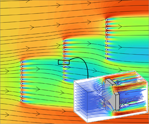
In the previous paragraph, the centre of the membrane was used to compute one set of approximate values of the tensors $\bar {M}_{ij}$ and $\bar {N}_{ij}$ in place of $1/\epsilon$ (i.e. one for each microscopic cell). Flow and geometry configurations of industrial interest are generally more complicated. We introduce a clustering algorithm in our macroscopic simulation workflow to automate the choice of a subset of flow conditions (i.e. of the $\mathcal {P}$ quantities) which can approximate the real, cell-wise distribution of $\mathcal {P}$. Given a set of length $N$ of the flow quantities $\mathcal {P}$, we divide $\mathcal {P}$ into $K \leq N$ clusters in which each element belongs to the cluster with the nearest centroid. We thus represent the cluster using its centroid. Several algorithms for splitting datasets into clusters have been proposed in the literature, see Bishop (Reference Bishop2006) for a review. Testing their relative performance in the present case goes beyond the scope of this work. For this reason, as an example, we choose the K-Means++ (Arthur & Vassilvitskii Reference Arthur and Vassilvitskii2007), implemented in Matlab 2023a. This algorithm splits a given set of data into a user-defined number of clusters according to a notion of distance, Euclidean in the present case. The optimal number of clusters can be found using some heuristic procedures, like the ‘elbow rule’ (Tibshirani, Walther & Hastie Reference Tibshirani, Walther and Hastie2001), but the cluster distribution is sufficiently evident in this case that the iterative procedure can be avoided. Figure 23(a) shows the considered flow configuration. It consists of three identical membranes composed of circular inclusions with spacing $\epsilon =0.1$, immersed in a free stream at $Re_L=500$. Velocity magnitude iso-levels and velocity streamlines are presented in panel ($a$). On the top and bottom sides of the domain, a no-slip boundary condition is applied. The leftmost membrane is fully exposed to the flow, as well as the top portions of the other two membranes, while the bottom portions experience milder flow conditions. Panel ($b$) shows that the data are clustered in three or four blocks, corresponding to the different flow conditions at the cell level. By computing the microscopic cases using the $\varSigma _{ij}^{\mathbb {U},\mathbb {D}}$ of each cluster centroid, we solve the corresponding macroscopic computation. A comparison of the velocity at the membranes in the full-scale solution and the clustered variable advection closure macroscopic solution is presented in figure 24. The prediction based on the four clusters is satisfactory compared with the full-scale solution, with minor discrepancies only in the tangential velocity of the red cluster. In terms of required computational resources, on a laptop with one INTEL i9-10900HK CPU (8 cores, 2.40 GHz) and 32 GB of RAM, a microscopic variable advection closure simulation has a run-time of up to 3 min, while a macroscopic simulation takes approximately 1 min. The clustering step proposed in this section has reduced the number of microscopic problems from $30$ to $4$ cases per iteration, which translates into a microscopic iteration step $7.5$ times faster. In general, if we suppose that the number of iterations and the number of clusters at each iteration are ${O}(1)$, while the number of microscopic cases to run at each iteration without clustering is ${O}(1/\epsilon )$, then clustering makes the iterative procedure ${O}(1/\epsilon )$ times faster. For the cases proposed in this work, a few iterations were needed for convergence: for $\epsilon Re_L$ of order $10$, generally, $1{-} 2$ iterations are sufficient, while for $\epsilon Re_L$ of order $100$, we need 5–6 iterations.

Figure 23.

($a$) Contours of velocity magnitude and streamlines (red) in the full-scale solution for $\alpha =90^{\circ }$, $\epsilon =0.1$ and $Re_L=500$. Each of the three identical membranes contains ten circular solid inclusions of porosity $0.7$ and spacing $\epsilon$. Inclusions $1$, $11$ and $21$ are located in $(0,0),(L,0.5L)$ and $(2L,L)$, respectively. The domain extent is $x_1\in [-1.5L,5.5L]$ and $y\in [-1.5L,3.5L]$. No slip is imposed on the top and bottom sides of the domain, while $(u_1,u_2)=(1,0)$ is imposed on the leftmost side and $\varSigma _{ij}n;j=0$ on the rightmost side of the domain. Cells are numbered from bottom to top and left to right (red text). ($b$) A possible clustering choice for the cells on the membrane obtained using the Matlab k-Means algorithm. Each cluster is visualized in a different marker and colour. Black markers represent the centroids of each cluster. Here, $\varSigma _{tn}^{\mathbb {D}}$ is close to zero, thus it does not affect the results and it is hence not shown. Black numbers refer to corresponding cells in panel ($a$).

Figure 24.

(a–c) Normal and (d–f) tangential velocity components on the centreline of each membrane. Black dots represent cell-averaged values of the full-scale solution, green lines represent the unclustered variable advection closure model and red lines are the clustered variable advection closure model. (g–i) Pressure values sampled at $\pm \epsilon /2$ from each centreline in the full-scale solution (full black line) and corresponding values for the unclustered variable advection closure model (green) and clustered variable advection closure (red) sampled on the corresponding sides of the fictitious interfaces. Panels ($a$,$d$,$g$) refer to the leftmost membrane, panels ($b$,$e$,$h$) to the central one and panels ($c$,$f$,$i$) to the rightmost membrane in figure 23(a).

Concerning the case proposed in figure 23, this case reaches a steady state in approximately $100$ time units. In a laptop with one INTEL i9-10900HK CPU ($8$ cores, $2.40$ GHz) and $32$ GB of RAM, the full-scale simulation (${\sim }270k$ degrees of freedom, kDOFs) has a runtime of approximately 310 s. The runtime of the macroscopic simulation sums up as follows: approximately $5$ s for a single initial Stokes microscopic problem, 80 s for the initial variable advection microscopic problem ($\sim$140 kDOFs), initialized with the Stokes solution, approximately $35$ s for each of the following variable advection microscopic problems, initialized with the previous solution. A single macroscopic solution ($\sim$55 kDOFs) takes approximately $10$ s. The problem requires three iterations (initialization included) and can be accurately approximated with four clusters for the microscopic problems. The total runtime for the macroscopic simulation is $5\ \textrm {s}+80 \textrm {s}+2\times 4\times 35\ \textrm {s}+3\times 10\ \textrm {s}=395\ \textrm {s}$. In the present case and from a total runtime point of view, using the macroscopic model does not imply a substantial computational gain. However, we should consider that:

1. (i) the macroscopic simulation is $\epsilon$-insensitive, i.e. its computational cost does not depend on the ratio between the pore and the membrane scales, whereas the full-scale simulation depends mainly on $\epsilon$, since it requires resolving all details of the microstructure;

2. (ii) in the macroscopic simulation, there are no mesh expansion-ratio-related problems, whereas it can be the case for the full-scale simulation, in particular, when $\epsilon$ is low or the microstructure has a non-trivial shape;

3. (iii) the RAM usage in the macroscopic case is reduced compared with the full-scale simulation since the iterative procedure splits the microscopic and macroscopic simulations;

4. (iv) most of the difference in runtime between the macroscopic and full-scale simulations stems from the microscopic coupling step. Creating a database of geometries and advective-velocity conditions or finding a surrogate model for them could further reduce the computational cost of the macroscopic simulation, making it of the order of the single macroscopic step in the coupling procedure.

These factors suggest that there is a gain in computational effort in using the present model when: (i) the scale separation is extreme (i.e. small $\epsilon$); (ii) the details of the microstructure require a non-negligible effort in preparing the mesh; (iii) the advective velocities are close to some representative mean value; and (iv) the RAM usage is limited. An even more significant gain is expected with surrogate models based on a large dataset of microscopic simulations.