2. AN INFEASIBLE EFFICIENT ESTIMATOR

Suppose that we have a sample {(X₁,Y₁),…,(X_n,Y_n)}, where

, from the nonparametric regression model (1.1). The objective is to estimate m₁(x) at some interior point x more efficiently than some conventional approach and to provide tight confidence intervals for such estimates. Noticing that the error terms in (1.1) are correlated, the conventional nonparametric estimator for m₁(x) does not take into account the correlation structure and thus is supposed to be dominated by some more efficient estimators. Nevertheless, the error terms in the transformed model (1.2) are uncorrelated. Equation (1.2) is also a valid regression equation by assumption. Let U_t−1 ≡ (U_t−1,…,U_t−d2). If m₂(U_t−1) were known, a nonparametric regression of Y_t − m₂(U_t−1) on X_t would be more efficient in the sense of mean squared errors than the nonparametric regression of Y_t on X_t. In this paper, we give asymptotic analysis based on the local polynomial procedure. See Fan (1992) and Fan and Gijbels (1996) for discussion on the attractive properties of local polynomials.

For any data set

, the local polynomial regression of

on X_t of order q can be obtained from the multivariate weighted least squares criterion:

where K₀ is a nonnegative kernel function on

and h₀ = h₀(n) is a scalar bandwidth sequence. Here, we use the notation of Masry (1996a, 1996b):

. The term θ_j = θ_j(x) = (1/j!)(∂^|j|m₁(x)/∂^j₁x₁…,∂^j_d1x_d1), where

. Let

, where

is the minimizing intercept in (2.1) with

, and let m₁(x) be the corresponding estimator when

. For simplicity, we suppose that

, with k₀ being the univariate kernel function. For later use, we denote

where θ = θ(x) is a collection of all the parameters θ_j, 0 ≤ |j| ≤ q, in a lexicographical order introduced subsequently. In particular, the first element in θ is denoted as θ₀ = θ₀(x) throughout our presentation.

Following the notation of Masry (1996a, 1996b), let N_l = (l + d₁ − 1)!/(l!(d₁ − 1)!) be the number of distinct d₁-tuples j with |j| = l. Arrange the N_l d₁-tuples as a sequence in a lexicographical order (with highest priority to last position so that (0,0,…,l) is the first element in the sequence and (l,0,…,0) is the last element) and let φ_l⁻¹ denote this one-to-one map. For each j with 0 ≤ |j| ≤ 2q, let

, and define the N × N-dimensional matrices M and Γ and N × N_q+1 matrix B, where

, by

where M_i,j and Γ_i,j are N_i × N_j-dimensional matrices whose (l,r) elements are, respectively, μ_{φi(l)+φj(r)} and υ_{φi(l)+φj(r)}. Note that the elements of the matrices M = M(K₀,q) and Γ = Γ(K₀,q) are simply multivariate moments of the kernel K₀ and K₀², respectively, and the matrix B = B(K₀,q) depends on the kernel and the order of the local polynomial we use. In addition, we arrange the N_r elements of the derivatives

as an N_r × 1 column vector m₁^(r)(x) in the lexicographical order.

The following theorem gives the asymptotic distribution of m₁(x) and shows that it is asymptotically more efficient than

.

THEOREM 2.1. Suppose that (1.2) holds. Then, under Assumption A in the next section, we have

where [A]_0,0 signifies the upper-left element of matrix A, M = M(K₀,q), Γ = Γ(K₀,q), and B = B(K₀,q).

Theorem 2.1 can be proved under much weaker assumptions, and it shows that the bias of the estimator m₁(x) is the same as that of the conventional qth-order local polynomial estimator

and the variance of m₁(x) is smaller than that of

.

It is straightforward to show that

.

. Let

. Then m₁(x) has a variance σ_ε²∥K₀∥₂²/f_X(x), and hence it is more efficient than the traditional local linear estimator

, which has variance σ_U²∥K₀∥₂²/f_X(x), where σ_U² = var(m₂(U_t−1)) + σ_ε². Therefore, the relative efficiency of the proposed estimator relative to the standard estimator in purely variance terms is σ_ε²/σ_U² ≤ 1. For example, when U_t = αU_t−1 + ε_t, we have σ_ε²/σ_U² = (1 − α²), which is strictly less than one except when α = 0. The percentage efficiency gain is less if measured in mean squared errors than in variances, but the two relative efficiencies are monotonically related.

We can make the comparison at the respectively optimal bandwidths. By Masry (1996a), the optimal bandwidth for estimating m₁(x) by

is given by h_0,opt = {(σ_U² d₁ [M⁻¹ΓM⁻¹]_0,0)/(2(q + 1){[M⁻¹Bm₁^(q+1)(x)]_0,0}²)}n^{−1/(2q+2+d₁)}. For m₁ the optimal bandwidth is the same as that for

but with σ_ε² in place of σ_U², and hence it is smaller. With this, one can obtain the formula for the mean squared errors when the optimal bandwidth is used.

We call m₁(x) an “oracle” estimator because its definition uses knowledge that only an oracle could have. A variety of smoothing paradigms could have been chosen here, and each will result in an “oracle” estimate. See Section 4 for more discussions.

3. A FEASIBLE EFFICIENT ESTIMATOR

In practice, m₂(·) is unknown and U_t−1 = (U_t−1,…,U_t−d2)′ is not observed. In this section we propose a feasible estimator by substituting a suitable pilot estimator of m₂(·) in (2.2) and replacing U_t−1 by the residuals obtained from regressing Y_t on X_t only. The proposed three-step estimation procedure is as follows.

1. Obtain a preliminary consistent estimator of m₁ by qth-order local polynomial smoothing Y_t on X_t with corresponding kernel K₁ and bandwidth sequence h₁ = h₁(n). Denote the preliminary estimates as

and calculate the estimated residuals

for t = 1,…,n.

⁴

Noting that we need to obtain

for all t = 1,…,n, we can tell that the Nadaraya–Watson kernel estimator is less desirable than the local polynomial estimator: we need to correct the boundary bias in the case where {X_t} is compactly supported or apply some trimming techniques otherwise. See Fan and Gijbels (1996) or Pagan and Ullah (1999) for more comparisons between the two types of estimators.

2. Obtain a consistent estimator of m₂ by pth-order local polynomial smoothing

on

with corresponding kernel K₂ and bandwidth sequence h₂ = h₂(n). Denote the estimates as

for t = d₂ + 1,…,n.

3. Replace m₂(U_t−1) in (2.2) by

to obtain

where

for some constant b = b(n) > 0 and

is the nonparametric kernel estimator for the density f_U of U_t−1 with bandwidth h₂ and kernel K₂ based on the residual series

. Let

minimize

and let

be our feasible estimate of m₁(x).

Like Robinson (1988) and Hidalgo (1992), we use

to trim out small values of

to get a desirable result for

. When U_t−1 has a compact support, m₂ can be estimated consistently over its full support by the local polynomial regression. So there is no need for trimming in this case.

The preceding procedure may be iterated to achieve better finite-sample performance in practice. We shall show subsequently that, under appropriate assumptions, the proposed estimator

is asymptotically equivalent to the infeasible estimator m₁(x). To facilitate the asymptotic analysis, let W_t = (X_t′,U_t−1′)′. We denote the densities of X_t, U_t−1, and W_t by f_X, f_U, and f_W, respectively. We make the following assumptions on the error terms, regressors, kernel functions, and bandwidth sequences.

Assumption A.

1. The kernels K_i,i = 0,1,2, satisfy

, where d₀ ≡ d₁ and k_i, i = 0,1,2, are bounded, symmetric about zero, and of compact support [−c_i,c_i] and satisfy the property that

. The functions H_ij(u) = u^jK_i(u) for all j with 0 ≤ |j| ≤ 2p + 1 for i = 2, and 0 ≤ |j| ≤ 2q + 1 for i = 0 and 1, are Lipschitz continuous. The first and second partial derivatives K₂⁽ⁱ⁾(u), i = 1,2, of K₂(u) satisfy ∫∥u^jK₂⁽ⁱ⁾(u)∥du < ∞ for 0 ≤ |j| ≤ 2p. The functions

for all j with 0 ≤ |j| ≤ 2p are Lipschitz continuous.

2. The strictly stationary process {(X_t′,U_t)′} is strong mixing with mixing coefficients α(j) that satisfy

for some δ > 0. The term f_X is Lipschitz continuous and bounded away from zero on its compact support. The first- and second-order partial derivatives of f_U are continuous and bounded on its support. The density f_W of W_t and the joint densities f_t1,…,tl(·,…,·) of (V₀,V_t1,…,V_tl) (1 ≤ l ≤ 5) are continuous and bounded where V_t ≡ (X_t′,X_t−1′,…,X_t−d2′,U_t−1′,ε_t)′.

Assumptions A1–A3 are comparable with Conditions 1–3 in Masry (1996a) except that our assumptions are a bit stronger than his. Unlike Li and Wooldridge (2002), who assume a β-mixing condition, which is handy for applying a result of Yoshihara (1976), we assume a strong mixing condition, which suffices to use the Davydov inequality (Bosq, 1996, p. 19) and one lemma due to Gao and King (2002) for U-statistics. The differentiability of A3 ensures a Taylor expansion to appropriate orders. Although A4 is a high-level assumption, it includes the stationary linear or nonlinear AR processes of finite order. If {U_t} is geometrically ergodic with its initial measure equal to its invariant measure, then {U_t} is strictly stationary. Primitive conditions on the geometric ergodicity of nonlinear autoregressive processes can be found from Appendix A1.4 of Tong (1990).

Assumption A5 looks complicated and deserves some comment. Let

, and I_t = 1{f_U(U_t−1) > b}. Then by Masry (1996b) and Hansen (2004),

if {U₁,…,U_n} were used in forming

. Assumptions A5(i) and (ii) require that the bias and variance terms in the first and second estimation stage should be o(n^−1/2h₀^{−d₁ /2}). Because {U₁,…,U_n} is not observed and

is used instead in forming

, there are compound estimation errors associated with the first two-stage estimation. We restrict them to be small in Assumptions A5(iii) and (iv): h₂⁻¹v_1n = o(1), h₂⁻¹b⁻²v_2n = o(1), h₂⁻¹b⁻²v_1n v_2n = o(n^−1/2h₀^{−d₁ /2}), b⁻¹h₂^pv_1n = o(n^−1/2h₀^{−d₁ /2}), where the appearance of h₂⁻¹ is due to the use of Taylor expansion in our proof. The last part of Assumption A5 will facilitate the proof. Like Hansen (2004), one can set b ∝ (ln n)^−1/2 and consider the case when p = q = 1. If d₁ = d₂ = 1, one can set h₀ ∝ n^−1/5, h₁ ∝ n^−1/4, and h₂ ∝ n^−1/4; if d₁ = 1 and d₂ = 2, one can set h₀ ∝ n^−1/5, h₁ ∝ n^−1/4, and h₂ ∝ n^−1/5; if d₁ = 2 and d₂ = 1 or 2, one can set h₀ ∝ n^−1/6, h₁ ∝ n^−1/5, and h₂ ∝ n^−1/4 or h₂ ∝ n^−1/5, respectively, etc.; then Assumption A5 is satisfied. When d₁ = d₂, undersmoothing is needed to achieve bias reductions in the first- and second-stage estimations, which is familiar from the multistep nonparametric estimation literature. In contrast, when d₂ < d₁, undersmoothing may not be required in the second-stage estimation. When f_U has a compact support and is bounded away from zero on its support, the trimming technique is not needed. See Remark 7 in Section 4.

THEOREM 3.1. Under Assumption A,

Remark 1. We have a sort of “oracle” property here: the feasible estimator

is asymptotically equivalent to m₁(x) and hence is more efficient than

. Therefore

should be preferred to

. The asymptotic normal distribution given by Theorem 3.1 can be used to calculate pointwise confidence intervals for estimators described here. To do this we require an estimation of the asymptotic variance. The procedure is standard, and we omit it for brevity.

Remark 2. It is worth mentioning that our three-stage approach has a close analogy with the well-known prewhitening method in the time series literature. See Press and Tukey (1956), Andrews and Monahan (1992), and more recently Xiao et al. (2003). Also, our efficiency gain may not require the correct specification of m₂ (or the correct choice of d₂) in the second stage. Interestingly, for any invertible MA process or strictly stationary AR process, the proposed estimator has an efficiency gain over the conventional one-step local polynomial estimator. To see this more clearly, suppose U_t = (1 − 0.7L)ε_t, where L is the lag operator. The process is invertible, so that we can write it as the AR(∞) process:

. Now if we fit a misspecified nonlinear AR(1) model to the AR(∞) process {U_t} : U_t = m₂(U_t−1) + e_t, where e_t ≡ U_t − E(U_t|U_t−1), we can tell that var(e_t) < var(U_t). So even for this misspecified model, the variance of our third-stage estimator is proportional to var(e_t), which is strictly smaller than the variance of the preliminary estimator (proportional to var(U_t)). Though not presented here the efficiency gain in such misspecified models was verified in a separate study through Monte Carlo simulations.

Remark 3. Horowitz, Klemela, and Mammen (2002) obtained asymptotic minimax results for estimating additive components in nonparametric regression models under the assumption that the error term is Gaussian. Fan, Gasser, Gijbels, Brockmann, and Engel (1997) showed that, with an appropriate choice of the bandwidth matrix and the kernel function, the univariate local polynomial regression estimator and the multivariate local linear regression estimator achieve the asymptotic linear minimax risk. To apply the latter result to our context, we assume for clarity that q = 1 and that the regression function m₁ is in the class

where C is a positive definite (d₁ × d₁) matrix. Heuristically speaking, this class includes regression functions that have a Hessian matrix bounded by C. If we choose the last-stage bandwidth and kernel function according to equation (3.1) and Theorem 3.1 of Fan et al. (1997), respectively, the resulting estimator

will be minimax efficient. Although minimax efficiency is an important property in theory, it is hard to work with and even harder to justify (cf. Linton, 2000). For this reason, we do not stress the minimax efficiency of our estimator.

4. MORE EFFICIENT ESTIMATION BASED ON GENERAL CRITERION FUNCTIONS

As Linton (2000) remarked, the notion of efficiency in nonparametric models is not as clear and well understood as it is in parametric models. One example he gave is that pointwise mean squared error comparisons do not provide a simple ranking between estimators such as kernels, splines, and nearest neighbors. Our purpose is to measure our procedure against the given infeasible (“oracle”) procedure for estimating m₁(x) based on the knowledge of m₂(·) and show that the estimator of m₁(x) based on our procedure is more efficient than the estimator obtained by ignoring m₂(·). This result does not pertain to the least squares criterion function only.

Like Linton (2000), we can extend the results in preceding sections and work with criterion functions motivated by the likelihood function of a complete specification of the conditional distribution of Y_t given W_t ≡ (X_t′,U_t′)′ along with the additive restriction (1.2). In the following discussion, we shall write w ≡ (x′,u′)′. We assume that the conditional distribution of Y_t given W_t = w comes from the one-parameter linear exponential family (e.g., Gourieroux, Monfort, and Trognon, 1984), admitting a density with respect to some fixed measure μ:

where A(·), B(·), and C(·) are known functions on the real line and

, a suitable parameter space, is the mean of the distribution whose density is P(y,m). Equation (4.1) suggests the following class of criterion functions:

where C_t(θ) = C(m₂(U_t−1) + [sum ]_0≤|j|≤q θ_j(X_t − x)^j), A_t(θ) = A(m₂(U_t−1) + [sum ]_0≤|j|≤q θ_j(X_t − x)^j), and B(Y_t) is absent from (4.2) because it does not depend on θ. Let

maximize Q_n(θ) and let

be our infeasible estimate of m₁(x). We have the following result.

THEOREM 4.1. Suppose that (1.2) holds and the functions A(·) and C(·) have bounded continuous derivatives up to order max(q + 1,3) over any compact interval. Then, under Assumption A, we have

where a(x) = a₂(x)/[a₁(x)]², a₁(x) = ∫C′(m₁(x) + m₂(u)) f_W(x,u) du, and a₂(x) = ∫C′(m₁(x) + m₂(u))²f_W(x,u) du.

Remark 4. The preceding theorem indicates that ignoring m₂(·) will result in a loss of efficiency in estimating m₁(·) for a general class of criterion functions. Corresponding to each density P (see (4.1)), we have an estimator, m₁⁺(x), for m₁(x) that is obtained from maximizing (4.2) when m₂(U_t−1) is absent in the definitions of A_t(θ) and C_t(θ). The term m₁⁺(x) will have the same bias as

but the variance that is proportional to σ_U². Thus m₁⁺(x) is dominated by

in terms of both variance and mean squared error. For example, if we choose the density P to be normal with mean m and variance 1, then

. From the preceding section, we know that m₁(x) is more efficient than the conventional one-step local polynomial estimator

.

Remark 5. From the proof of the preceding theorem ((A.5)–(A.9) in particular), we can see that a stronger conclusion can be drawn: all derivatives of m₁(x) up to order q can be estimated more efficiently in the procedure of obtaining

than in the procedure of obtaining m₁⁺(x). Because our primary interest is the efficient estimation of m₁(x), we state the theorem as it is.

Like m₁(x) introduced before,

is an “oracle” estimate. In practice, we can follow the procedure in Section 3 to obtain a feasible estimator for m₁(x). Specifically, we replace m₂(U_t−1) in (4.2) by

to obtain

where

. Let

maximize

in (4.3) and let

be our feasible estimate of m₁(x). A result similar to Theorem 3.1 can be stated as follows.

THEOREM 4.2. Suppose that the functions A(·) and C(·) have bounded continuous derivatives up to order max(q + 1,3) over any compact interval. Then, under Assumption A, we have

where a(x) is defined in Theorem 4.1.

Remark 6. This says that

is asymptotically equivalent to

and thus more efficient than m₁⁺(x). The expression

is constructed by the three-step procedure, implying that the estimation of the infinite-dimensional nuisance parameter m₂(·) has no impact on the limiting distribution of

. This is not generally the case in parametric estimation problems, unless there is some orthogonality between the estimating equations. One important reason for our procedure to work is that the bias from the first two-step estimation can be made asymptotically negligible by undersmoothing in the first one or two stages. As before, if we choose the density P to be normal with mean m and variance 1, then

. From the preceding section, we know that

is more efficient than the conventional one-step local polynomial estimator

.

Remark 7. Recently, Hansen (2004) provides a uniform convergence result for a sample average functional, which can easily be used for density and regression estimation with infinite support. Applying Theorem 3 of Hansen (2004), one can easily show

The preceding result plays a key role in our proof of Theorem 4.2. It is easy to see that the local polynomial estimation of m₂ can be replaced by the standard nonparametric kernel regression. We stick to the local polynomial estimation because there is no need for trimming when f_U is compactly supported.

5. MONTE CARLO SIMULATIONS

In this section we first address the issue of determining the order d₂ in the second-stage estimation. Then we investigate the proposed estimator

on simulated data and compare it with the conventional one-step local polynomial estimator

and the conventional kernel estimator.

5.1. Choice of d₂

In the preceding sections we assume that the order of serial correlation d₂ is known. In practice, however, d₂ is generally unknown. Recently Gao and Tong (2004) have developed a novel cross-validation-based model selection procedure for semiparametric nonlinear time series when all regressors are observables. One can in theory extend their results by allowing for nonparametrically generated regressors. However, the theoretical investigation of this problem can be quite tedious. So we use simulations to examine whether the Gao and Tong method is useful in our context.⁵

The authors are thankful to a referee for suggesting the use of the Gao and Tong (2004) simulation procedure.

We consider a small class of data generating processes (DGPs) for the error process {U_t}, including both linear and nonlinear AR(1) processes and two linear AR(2) processes:

where φ(·) is the standard normal density function, {ε_t} is i.i.d., and ε_t is equal to the sum of 100 independent random variables each uniformly distributed on [−0.1, 0.1]. According to the central limit theorem (CLT), we can treat ε_t as being nearly a normal random variable with truncated support on [−10, 10] (see Yao and Tong, 1994, p. 59). DGPs 1, 5, and 6 allow us to examine the effect of linear dependence on the proposed estimator. DGPs 2–4 are nonlinear processes. The stationary and mixing conditions for the linear processes can be justified easily, and those for the nonlinear processes can be verified by using existing results from Masry and Tjøstheim (1995, 1997). In all cases, the dependent variables are generated according to Y_t = m₁(X_t) + U_t, where m₁(X_t) = 5 exp(X_t)/(1 + exp(X_t)) and {X_t} is i.i.d. uniform on [−0.5, 0.5] and is independent of the process {ε_t}. Simple algebra shows that var(m₁(X_t)) = 0.127, which is comparable to var(ε_t) ≃ 0.333.

We first obtain a local linear estimator of m₁ by choosing q = 1, the Gaussian kernel K₁(u) = (2π)^−1/2 exp(−u²/2), and the rule of thumb bandwidth for Gaussian kernel

, where

is the sample standard error for {X_t}_t=1ⁿ. We denote the local linear estimates as

and calculate the residuals

for t = 1,…,n. Then we apply the procedure of Gao and Tong (2004) to choose the order d₂ based on

.

To be specific, we consider the case where U_t−1, U_t−2, and U_t−3 are selected as candidate regressors in generating U_t. Like Gao and Tong (2004), we split the observed data set

into two parts:

, where S is a subset of {4,5,…,n} containing n_v integers and S^c is its complement containing n_c integers: n_c + n_v = n − 3. The basic idea of Gao and Tong is to use the “construction” data

to run the regression of

on potential candidate regressors chosen from R_t and then to assess the prediction error by using the data

, treated as if they were future values.

Let

denote all nonempty subsets of {1,2,3}. For any

, denote R_t,D as a column vector consisting of

such that i ∈ D. Let K_D be a multivariate kernel function defined on

be a bandwidth parameter. Denote

. The average squared prediction error is

analogous to equation (2.9) in Gao and Tong (2004), where w(·) is a weighting function. In the special case where n_v = 1, we get the conventional leave-one-out cross-validation function (CV1). Let us randomly draw a collection

of m subsets of {4,5,…,n} that have size n_v. Let

and denote

, where H_D^c is a set of bandwidth parameters. Under suitable conditions, we conjecture that with probability converging to one,

will pick up the right regressors in R_t.

We choose K_D, H_D^c, m, and n_c according to Section 3.1 in Gao and Tong (2004): K_D is a product of |D| standard normal kernels, H_D^c ≡ [0.1n_c^−2/9, 3n_c^−1/9], m = n − 3, and n_c = [lceil ](n − 3)^0.9[rceil ], the largest integer part of (n − 3)^0.9. We use

, where

is the sample standard error for

. To save time, we specify

, and we choose h ∈ H_D^c by discretizing H_D^c with 50 equally spaced points. Table 1 reports the relative frequencies that each element of

is selected by using the Monte Carlo cross validation (MCCV) criterion function.

Relative frequencies based on the semiparametric MCCV order selection of Gao and Tong (2004)

Table 1 shows that when the true order (d₂) of the time series {U_t} is 1, the MCCV procedure of Gao and Tong (2004) can pick up the right order even when the sample size is fairly small (n = 200) given the fact that three-dimensional densities have to be estimated in the selection procedure. When d₂ = 2, the success of the procedure depends on the persistence in the data: for low persistent data (DGP 5), the Gao and Tong procedure still works well for n as small as 200, but for highly persistent data (DGP 6), a large sample (n ≥ 500) is required.

5.2. Efficiency Comparison

Now we suppose that the right number of lags, d₂, has been chosen and investigate the proposed estimator

on simulated data and compare it with the conventional one-step local polynomial estimator

and the conventional kernel estimator,

. We do not try to optimize the performance of either the conventional estimators or our own. Rather, we take what are fairly common choices, in real applications, of bandwidth sequences and kernels and demonstrate that even with these implements there are significant finite-sample gains to be made. We choose the same Epanechnikov kernel in estimating

: K_i(u) = 0.75(1 − u²)1(|u| ≤ 1), i = 0,1,2. Note that the error term has a compact support; we do not use the trimming device in our simulations.

For bandwidth sequences, noticing that only h₀ shows up in the limiting distribution of our more efficient estimator, we recommend choosing h₀ based upon the nonparametric leave-one-out cross-validation method. To be specific, let

; we choose h₀ to be

where

is obtained as

by deleting the tth observation, w(X_t) is defined analogously as in Section 5.1, and

is obtained by grid search over the interval

in 50 steps. We shall use the same bandwidth

in obtaining

as in the third step of obtaining

.

To obtain

, we also need to choose h₁ and h₂ in the first two-stage estimation. As we shall see, our efficient results are not sensitive to the choice of these two bandwidth parameters, and so we recommend some rules of thumb based on the optimal bandwidth for nonparametric kernel density estimation. It is well known that the optimal bandwidth for estimating a one-dimension density with the Epanechnikov kernel is given by

. So when d₁ = 1 and q = p = 1, by rule of thumb we can set

, where we have imposed undersmoothing conditions. This choice of h₁ and h₂, together with the choice of

, will meet Assumption A5 for d₂ = 1, 2, or 3, where we conjecture that this data-driven bandwidth selection does not alter the validity of our theorems. If d₁ ≥ 2, we can modify the rule correspondingly, e.g., set

, where one should understand that h₁ is a diagonal matrix and that

is a diagonal matrix with the standard deviation of, say, {X_i,t} in the (i,i)th place. In the following experiment (d₁ = 1, d₂ = 1 or 2), we set

, where c ∈ {1, 2, 4}, and consider three sample sizes: n = 100, 200, and 500.

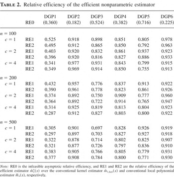
First we consider the estimation of m₁(x) at the interior point x = 0 and report in Table 2 the relative efficiency: the ratio of average mean squared errors over 500 replications. In the table, row RE1 reports the relative efficiency of the proposed efficient estimator

over the conventional kernel estimator

, and row RE2 reports the relative efficiency of the proposed efficient estimator

over the conventional local polynomial estimator

. For comparison purposes, we also report in Table 2 the infeasible asymptotic relative efficiency (RE0) calculated based upon the asymptotic variance of

. It is worth mentioning that the second derivative of m₁(x) at x = 0 is 0. So RE0 is also the asymptotic relative efficiency based on the mean squared error of

at x = 0.

Relative efficiency of the efficient nonparametric estimator

We summarize some general findings from our simulation experiments. (1) The proposed efficient estimator performs very well across various DGPs under our investigation and across different c's that control the degree of smoothing in the first two-stage estimations. (2) In general, the more the serial dependence in the error process, the larger is the efficiency gain achieved. In particular, for the linear AR(1) processes, like Xiao et al. (2003), we find in a separate study that the relative efficiency first improves as the AR coefficient in absolute value increases and then degenerates as the coefficient approaches one. This suggests that a different asymptotic theory may apply when we have a near unit error process. (3) There are more substantial gains that can be achieved for negative serial dependence cases (DGP1) than for positive serial dependence cases (DGPs 2, 4–6). The RE1 and RE2 can reach RE0 in the case where the negative serial dependence is large (DGP1). (4) The relative efficiency generally improves when the sample sizes n increase from 100 to 200.

We also consider the estimation of m₁(x) over all sample points X₁,…,X_n and calculate the integrated relative efficiency (IRE) as the ratios of mean squared errors that are averaged over a smaller number of replications and over all data points. The results are qualitatively similar to the preceding analysis.