1 Introduction
Submerged jets become globally unstable, achieving a self-sustained oscillatory state, when their density is sufficiently smaller than that of their surroundings, as clearly evidenced by many experimental, theoretical and numerical studies. The phenomenon was first recognised thanks to the pioneering work of Monkewitz & Sohn (Reference Monkewitz and Sohn1988), who demonstrated the existence of a region of local absolute instability close to the injector of a turbulent heated jet by means of a quasi-parallel linear stability analysis. The global transition has been experimentally characterised in detail both for hot jets (Monkewitz et al. Reference Monkewitz, Bechert, Barsikow and Lehmann1990) and for light jets, where the density difference is due to the injection of fluid of smaller molecular weight than that of the ambient (Kyle & Sreenivasan Reference Kyle and Sreenivasan1993; Hallberg & Strykowski Reference Hallberg and Strykowski2006), and also by means of a number of local stability analyses which accounted for the origin of the phenomenon with increasing detail (Jendoubi & Strykowski Reference Jendoubi and Strykowski1994; Lesshafft & Huerre Reference Lesshafft and Huerre2007; Coenen, Sevilla & Sánchez Reference Coenen, Sevilla and Sánchez2008; Lesshafft & Marquet Reference Lesshafft and Marquet2010; Coenen & Sevilla Reference Coenen and Sevilla2012). These studies have been complemented by direct numerical simulations (Lesshafft, Huerre & Sagaut Reference Lesshafft, Huerre and Sagaut2007) that unambiguously demonstrated the link between the existence of locally absolutely unstable regions in the near field of low-density jets and the onset of global self-sustained oscillations.
Recently, several global linear stability analyses of submerged jet configurations, avoiding the quasi-parallel approximation, have been performed thanks to the availability of sufficient computational power and the development of appropriate numerical techniques. Nichols & Lele (Reference Nichols and Lele2011a ) pioneered the use of a global approach to study hot and cold compressible jets. Garnaud et al. (Reference Garnaud, Lesshafft, Schmid and Huerre2013a ,Reference Garnaud, Lesshafft, Schmid and Huerre b ) considered the case of constant-density incompressible jets, revealing that global modes are strongly affected by the domain length and the numerical discretisation, while the frequency response is robust and explains the origin of the preferred mode in globally stable jets. In contrast with the case of constant-density jets, the important experiments of Hallberg & Strykowski (Reference Hallberg and Strykowski2006) strongly suggest the existence of an isolated eigenmode responsible for the global transition for sufficiently low values of the Reynolds number. Isolated eigenmodes in low-density jets have indeed been detected by Nichols & Lele (Reference Nichols and Lele2010) for supersonic cases, and by Qadri (Reference Qadri2014) for a low Mach number configuration.
The main objective of the present work is to provide a detailed characterisation of the global stability properties of light
 $\text{He}/\text{N}_{2}$
laminar jets in the low Mach number limit, by means of modal and frequency response analyses. Two key questions addressed are whether there exists an isolated eigenmode that explains the experimentally observed transition in low-density jets, and what are the differences between the global stability properties of constant-density and low-density jets.
The paper begins with the mathematical formulation in § 2. In § 3 we study a slowly developing globally stable jet, followed by an analysis of a rapidly spreading helium jet in § 4. Finally, concluding remarks are given in § 5.
2 Formulation
We consider an axisymmetric laminar low-density
 $\text{He}/\text{N}_{2}$
jet, discharging with a constant flow rate
 $Q^{\ast }$
from an injector pipe with radius
 $R^{\ast }$
into an ambient of
 $\text{N}_{2}$
. The ratio of the density
 $\unicode[STIX]{x1D70C}_{j}^{\ast }$
of the jet and the ambient density
 $\unicode[STIX]{x1D70C}_{\text{N}_{2}}^{\ast }$
is given by
 $S=W_{j}^{\ast }/W_{\text{N}_{2}}^{\ast }$
. Here
 $W_{j}^{\ast }=[Y_{j}/W_{\text{He}}^{\ast }+(1-Y_{j})/W_{\text{N}_{2}}^{\ast }]^{-1}$
is the mean molecular weight of the jet mixture, determined by the initial mass fraction
 $Y_{j}$
of
 $\text{He}$
. In other terms, to obtain a jet with jet-to-ambient density ratio
 $S$
, an initial mass fraction
 $Y_{j}=(S^{-1}-1)/(W_{\text{N}_{2}}^{\ast }/W_{\text{He}}^{\ast }-1)$
of
 $\text{He}$
is injected. The viscosity
 $\unicode[STIX]{x1D707}_{j}^{\ast }$
of the jet can be related to
 $\unicode[STIX]{x1D707}_{\text{He}}^{\ast }$
and
 $\unicode[STIX]{x1D707}_{\text{N}_{2}}^{\ast }$
through Hirschfelder, Curtiss & Bird’s law (see Coenen & Sevilla Reference Coenen and Sevilla2012, (2.11)). Note that in the formulation dimensional quantities are indicated with an asterisk
 $^{\ast }$
. The jet exit values
 $\unicode[STIX]{x1D70C}_{j}^{\ast }$
,
 $\unicode[STIX]{x1D707}_{j}^{\ast }$
are used as scales for the dimensionless density
 $\unicode[STIX]{x1D70C}$
and viscosity
 $\unicode[STIX]{x1D707}$
, whereas the jet radius
 $R$
is used as the characteristic length scale, yielding the dimensionless cylindrical coordinate system
 $(x,r)$
. The velocity field
 $\boldsymbol{u}=(u,v)$
is non-dimensionalised with the mean velocity
 $U_{m}^{\ast }=4Q^{\ast }/(\unicode[STIX]{x03C0}{R^{\ast }}^{2})$
. All flow quantities are taken to be independent of the azimuth
 $\unicode[STIX]{x1D719}$
throughout this study; only axisymmetric perturbations are considered.
The Reynolds number of the jet is assumed to be large,
 $Re=\unicode[STIX]{x1D70C}_{j}^{\ast }U_{m}^{\ast }R^{\ast }/\unicode[STIX]{x1D707}_{j}^{\ast }\gg 1$
, resulting in a slender jet flow. The importance of buoyancy effects can be estimated through the Richardson number
 $Ri=(\unicode[STIX]{x1D70C}_{\text{N}_{2}}^{\ast }-\unicode[STIX]{x1D70C}_{j}^{\ast })g^{\ast }R^{\ast }/(\unicode[STIX]{x1D70C}_{j}^{\ast }{U_{m}^{\ast }}^{2})$
. For comparison with experiments, it is useful to write this as
 $Ri=Gr/Re^{2}$
, where
 $Gr=\unicode[STIX]{x1D70C}_{j}^{\ast }(\unicode[STIX]{x1D70C}_{\text{N}_{2}}^{\ast }-\unicode[STIX]{x1D70C}_{j}^{\ast })g^{\ast }{R^{\ast }}^{3}/{\unicode[STIX]{x1D707}_{j}^{\ast }}^{2}=(1/S-1)g^{\ast }{R^{\ast }}^{3}/\unicode[STIX]{x1D708}_{j}^{\ast }$
is a Grashof number. The latter only depends on the injector radius and the properties of the gas mixture, which usually do not vary within the same experimental campaign. For simplicity, we will neglect buoyancy effects, i.e. we will assume
 $Ri\ll 1$
, except for the comparison with experiments in § 4.2. Furthermore, for the description of the resulting jet flow it is assumed that the characteristic jet velocity
 $U_{m}^{\ast }$
is much smaller than the ambient speed of sound, so that the simplifications associated with the low Mach number approximation (Williams Reference Williams1985; Nichols, Schmid & Riley Reference Nichols, Schmid and Riley2007) can be applied. This implies that the density variations in the jet are only due to variations in molecular weight, and are not related to pressure variations. It also means that if the jet discharges with the same temperature as the ambient, the flow will remain isothermal everywhere, and the energy equation is not needed in the description. Furthermore, in the low Mach number limit, the viscous stress term that is proportional to the second coefficient of viscosity can be incorporated in the definition of the variable
 $p$
. This
 $p$
represents the pressure difference from the unperturbed ambient distribution, scaled with the characteristic dynamic pressure
 $\unicode[STIX]{x1D70C}_{j}^{\ast }{U_{m}^{\ast }}^{2}$
. The jet is then effectively described by the continuity, momentum conservation and species conservation equations,
 $$\begin{eqnarray}\displaystyle & \displaystyle \frac{\unicode[STIX]{x2202}\unicode[STIX]{x1D70C}}{\unicode[STIX]{x2202}t}+\unicode[STIX]{x1D735}\boldsymbol{\cdot }(\unicode[STIX]{x1D70C}\boldsymbol{u})=0, & \displaystyle\end{eqnarray}$$
 $$\begin{eqnarray}\displaystyle & \displaystyle \unicode[STIX]{x1D70C}\left(\frac{\unicode[STIX]{x2202}\boldsymbol{u}}{\unicode[STIX]{x2202}t}+\boldsymbol{u}\boldsymbol{\cdot }\unicode[STIX]{x1D735}\boldsymbol{u}\right)=-\unicode[STIX]{x1D735}p+\frac{1}{Re}\unicode[STIX]{x1D6FB}^{2}\boldsymbol{u}+Ri\frac{1-S\unicode[STIX]{x1D70C}}{1-S}\boldsymbol{e}_{x}, & \displaystyle\end{eqnarray}$$
 $$\begin{eqnarray}\displaystyle & \displaystyle \unicode[STIX]{x1D70C}\left(\frac{\unicode[STIX]{x2202}Y}{\unicode[STIX]{x2202}t}+\boldsymbol{u}\boldsymbol{\cdot }\unicode[STIX]{x1D735}Y\right)=\frac{1}{Re\,Sc}\unicode[STIX]{x1D735}\boldsymbol{\cdot }(\unicode[STIX]{x1D70C}\unicode[STIX]{x1D735}Y), & \displaystyle\end{eqnarray}$$
together with the relation between the mass fraction
 $Y$
of
 $\text{He}$
and the density
 $\unicode[STIX]{x1D70C}$
of the jet,
 $$\begin{eqnarray}\displaystyle Y=Y_{j}(1/\unicode[STIX]{x1D70C}-S)/(1-S). & & \displaystyle\end{eqnarray}$$
In (2.3) the Schmidt number
 $Sc=\unicode[STIX]{x1D707}_{j}^{\ast }/(\unicode[STIX]{x1D70C}_{j}^{\ast }{\mathcal{D}}^{\ast })$
is based on the values of the viscosity and density at the jet exit. For example, the two density ratios used in the present work,
 $S=0.143$
and
 $S=0.5$
, correspond to Schmidt numbers
 $Sc=1.69$
and
 $Sc=0.49$
, respectively. For simplicity, the variation of the viscosity with the composition is not taken into account in the conservation equations (2.1)–(2.3), and is thus neglected in the results, except for the comparison with experiments of § 4.2, where its influence is studied separately. To the latter aim, the viscous term in (2.2) is written as
 $Re^{-1}\unicode[STIX]{x1D735}\boldsymbol{\cdot }[\unicode[STIX]{x1D707}(\unicode[STIX]{x1D735}\boldsymbol{u}+\unicode[STIX]{x1D735}\boldsymbol{u}^{\text{T}})]$
and Hirschfelder’s law (see Coenen & Sevilla Reference Coenen and Sevilla2012, (2.11)) is used to relate the dimensionless viscosity
 $\unicode[STIX]{x1D707}=\unicode[STIX]{x1D707}^{\ast }/\unicode[STIX]{x1D707}_{j}^{\ast }$
to the mass fraction
 $Y$
.
2.1 Base flow
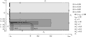
Schematic representation of the numerical domain. The boxed numbers on the boundaries indicate the level of refinement through the distance
 $h$
between discretisation points. The areas with different grid resolutions that are obtained in this manner are indicated by the grey shading.

As a base state for the linear stability analysis, a steady solution
 $(\bar{u},\bar{v},\bar{p},\bar{\unicode[STIX]{x1D70C}})$
of the low Mach number Navier–Stokes equations (2.1)–(2.3) is employed. The flow domain under consideration is depicted in figure 1. In order to mimic experimental conditions, a short injector pipe of length
 $x_{p}$
is included, bounded by a wall
 $\unicode[STIX]{x1D6E4}_{w}$
of thickness 0.02 that ends on a
 $5.7^{\circ }$
knife edge. At the pipe inlet
 $\unicode[STIX]{x1D6E4}_{i}$
a velocity profile
 $\bar{u}_{i}(r)$
is imposed, taken from a collection of profiles that is obtained by solving the laminar boundary-layer equations in a circular pipe (see Coenen & Sevilla Reference Coenen and Sevilla2012, § 2.1.1). Because the flow in the short injector pipe of the domain will further develop, the velocity profile
 $\bar{u}_{i}(r)$
at the inlet must be carefully chosen to obtain a certain desired velocity profile
 $\bar{u}_{0}(r)$
at the jet exit plane. We will characterise the latter profile through the inverse of its dimensionless momentum thickness
 $D/\unicode[STIX]{x1D703}_{0}$
, defined by
 $$\begin{eqnarray}\displaystyle \unicode[STIX]{x1D703}_{0}=\int _{0}^{\infty }\frac{\bar{u}_{0}(r)}{\bar{u}_{0}(0)}\left[1-\frac{\bar{u}_{0}(r)}{\bar{u}_{0}(0)}\right]\,\text{d}r, & & \displaystyle\end{eqnarray}$$
and scaled with the jet diameter
 $D=2R$
for consistency with Hallberg & Strykowski (Reference Hallberg and Strykowski2006). For the computations of the results of the present work a pipe length
 $x_{p}=3$
was used, with the exception of the transition points with
 $D/\unicode[STIX]{x1D703}_{0}>30$
of figure 12, for which a pipe length
 $x_{p}=1.5$
was used. It was verified that larger values of
 $x_{p}$
did not affect the results. The remaining boundaries of the flow domain are the axis
 $\unicode[STIX]{x1D6E4}_{a}$
, the lateral boundary
 $\unicode[STIX]{x1D6E4}_{t}$
and the downstream outlet boundary
 $\unicode[STIX]{x1D6E4}_{o}$
, as labelled in figure 1. Stress-free boundary conditions are imposed on the latter two. Because the jet entrains fluid through the lateral boundary, the density at that boundary must be fixed to
 $1/S$
to obtain the desired jet-to-ambient density ratio. The radial extent of the domain was set to
 $r_{max}=10$
, and it was checked that larger values did not change the results. The downstream extent
 $x_{max}$
does not influence the computation of the base flow, but it does affect various results of the stability analysis, as will be explained in detail in §§ 3 and 4; values in the range
 $40\leqslant x_{max}\leqslant 100$
were used. To summarise, the boundary conditions for the base flow are
 $$\begin{eqnarray}\displaystyle & \displaystyle \bar{u}-\bar{u}_{i}=\bar{v}=\bar{\unicode[STIX]{x1D70C}}-1=0\quad \text{on }\unicode[STIX]{x1D6E4}_{i}, & \displaystyle\end{eqnarray}$$
 $$\begin{eqnarray}\displaystyle & \displaystyle \bar{u}=\bar{v}=\boldsymbol{n}\boldsymbol{\cdot }\unicode[STIX]{x1D735}\bar{\unicode[STIX]{x1D70C}}=0\quad \text{on }\unicode[STIX]{x1D6E4}_{w}, & \displaystyle\end{eqnarray}$$
 $$\begin{eqnarray}\displaystyle & \displaystyle \bar{\unicode[STIX]{x1D70C}}-\frac{1}{S}=-\bar{p}\boldsymbol{n}+\frac{1}{Re}\boldsymbol{n}\boldsymbol{\cdot }\unicode[STIX]{x1D735}\binom{\bar{u}}{\bar{v}}=0\quad \text{on }\unicode[STIX]{x1D6E4}_{t} & \displaystyle\end{eqnarray}$$
 $$\begin{eqnarray}\displaystyle & \displaystyle -\bar{p}\boldsymbol{n}+\frac{1}{Re}\boldsymbol{n}\boldsymbol{\cdot }\unicode[STIX]{x1D735}\binom{\bar{u}}{\bar{v}}=0\quad \text{on }\unicode[STIX]{x1D6E4}_{o}, & \displaystyle\end{eqnarray}$$
 $$\begin{eqnarray}\displaystyle & \displaystyle \bar{v}=\unicode[STIX]{x2202}_{r}\bar{u}=\unicode[STIX]{x2202}_{r}\bar{\unicode[STIX]{x1D70C}}=0\quad \text{on }\unicode[STIX]{x1D6E4}_{a}, & \displaystyle\end{eqnarray}$$
where
 $\boldsymbol{n}$
is the outward normal vector on the boundary.
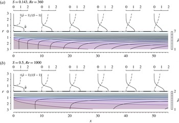
Radial profiles of axial velocity
 $\bar{u}$
and rescaled density
 $(\bar{\unicode[STIX]{x1D70C}}-1)/(S-1)$
at
 $x=0,10,20,30,40,50$
, together with streamlines and contours of the density field
 $\bar{\unicode[STIX]{x1D70C}}$
, for (a)
 $S=0.143$
,
 $Re=360$
,
 $D/\unicode[STIX]{x1D703}_{0}=24.3$
and (b)
 $S=0.5$
,
 $Re=1000$
,
 $D/\unicode[STIX]{x1D703}_{0}=24.3$
.

The governing equations are discretised using Taylor–Hood elements, quadratic (P2) for the density and velocity, and linear (P1) for the pressure, to satisfy the Ladyzenskaja–Babuška–Brezzi condition. The refinement of the unstructured mesh is controlled through the distance
 $h$
between discretisation points on the boundaries of the domain and on auxiliary lines, as indicated in figure 1. It was checked that the results were converged with respect to further mesh refinements. The steady base flow is computed using a Newton–Raphson method and the FreeFem
 $++$
software (Hecht Reference Hecht2012). Figure 2 shows the resulting base flow for the two cases that will be studied in detail in §§ 3 and 4:
 $S=0.143$
,
 $Re=360$
,
 $D/\unicode[STIX]{x1D703}_{0}=24.3$
and
 $S=0.5$
,
 $Re=1000$
,
 $D/\unicode[STIX]{x1D703}_{0}=24.3$
.
2.2 Direct eigenmodes
All experimental and numerical evidence indicates that the global instability in light jets gives rise to axisymmetric flow oscillations, and the present analysis therefore is restricted to axisymmetric disturbances. All flow quantities are independent of the azimuthal coordinate, and the azimuthal velocity is always zero. Small unsteady axisymmetric perturbations are introduced into the steady base flow as
 $(u,v,\unicode[STIX]{x1D70C},p)=(\bar{u},\bar{v},\bar{\unicode[STIX]{x1D70C}},\bar{p})+\unicode[STIX]{x1D700}(u^{\prime },v^{\prime },\unicode[STIX]{x1D70C}^{\prime },p^{\prime })$
. The evolution of these perturbations (primed quantities) is then governed to leading order by the equations (2.1)–(2.4), linearised around the base flow,
 $$\begin{eqnarray}\displaystyle & \displaystyle \unicode[STIX]{x1D735}\boldsymbol{\cdot }\boldsymbol{u}^{\prime }=-\frac{1}{Re\,Sc}\unicode[STIX]{x1D735}\boldsymbol{\cdot }\left(\frac{1}{\bar{\unicode[STIX]{x1D70C}}}\unicode[STIX]{x1D735}\unicode[STIX]{x1D70C}^{\prime }-\frac{\unicode[STIX]{x1D70C}^{\prime }}{\bar{\unicode[STIX]{x1D70C}}^{2}}\unicode[STIX]{x1D735}\bar{\unicode[STIX]{x1D70C}}\right), & \displaystyle\end{eqnarray}$$
 $$\begin{eqnarray}\displaystyle & \displaystyle \frac{\unicode[STIX]{x2202}\boldsymbol{u}^{\prime }}{\unicode[STIX]{x2202}t}+\bar{\boldsymbol{u}}\boldsymbol{\cdot }\unicode[STIX]{x1D735}\boldsymbol{u}^{\prime }+\boldsymbol{u}^{\prime }\boldsymbol{\cdot }\unicode[STIX]{x1D735}\bar{\boldsymbol{u}}+\frac{\unicode[STIX]{x1D70C}^{\prime }}{\bar{\unicode[STIX]{x1D70C}}}\bar{\boldsymbol{u}}\boldsymbol{\cdot }\unicode[STIX]{x1D735}\bar{\boldsymbol{u}}=-\frac{1}{\bar{\unicode[STIX]{x1D70C}}}\unicode[STIX]{x1D735}p^{\prime }+\frac{1}{Re}\frac{1}{\bar{\unicode[STIX]{x1D70C}}}\unicode[STIX]{x1D6FB}^{2}\boldsymbol{u}^{\prime }-Ri\frac{S}{1-S}\frac{\unicode[STIX]{x1D70C}^{\prime }}{\bar{\unicode[STIX]{x1D70C}}}\boldsymbol{e}_{x},\quad & \displaystyle\end{eqnarray}$$
 $$\begin{eqnarray}\displaystyle & \displaystyle \frac{\unicode[STIX]{x2202}\unicode[STIX]{x1D70C}^{\prime }}{\unicode[STIX]{x2202}t}+\bar{\boldsymbol{u}}\boldsymbol{\cdot }\unicode[STIX]{x1D735}\unicode[STIX]{x1D70C}^{\prime }+\boldsymbol{u}^{\prime }\boldsymbol{\cdot }\unicode[STIX]{x1D735}\bar{\unicode[STIX]{x1D70C}}-\frac{\unicode[STIX]{x1D70C}^{\prime }}{\bar{\unicode[STIX]{x1D70C}}}\bar{\boldsymbol{u}}\boldsymbol{\cdot }\unicode[STIX]{x1D735}\bar{\unicode[STIX]{x1D70C}}=-\frac{1}{Re\,Sc}\bar{\unicode[STIX]{x1D70C}}\unicode[STIX]{x1D735}\boldsymbol{\cdot }\left(\frac{1}{\bar{\unicode[STIX]{x1D70C}}}\unicode[STIX]{x1D735}\unicode[STIX]{x1D70C}^{\prime }-\frac{\unicode[STIX]{x1D70C}^{\prime }}{\bar{\unicode[STIX]{x1D70C}}}\unicode[STIX]{x1D735}\bar{\unicode[STIX]{x1D70C}}\right). & \displaystyle\end{eqnarray}$$
Assuming temporal normal-mode solutions
 $$\begin{eqnarray}\displaystyle (u^{\prime },v^{\prime },\unicode[STIX]{x1D70C}^{\prime },p^{\prime })=(\hat{u} ,\hat{v},\hat{\unicode[STIX]{x1D70C}},\hat{p})\text{e}^{-i\unicode[STIX]{x1D714}t}, & & \displaystyle\end{eqnarray}$$
the linearised equations can be written in the form of a generalised eigenvalue problem
 $$\begin{eqnarray}\displaystyle -\text{i}\unicode[STIX]{x1D714}{\mathcal{B}}\hat{\boldsymbol{q}}={\mathcal{L}}\hat{\boldsymbol{q}}, & & \displaystyle\end{eqnarray}$$
where
 $\hat{\boldsymbol{q}}(r,x)=[\hat{u} (r,x),\hat{v}(r,x),\hat{\unicode[STIX]{x1D70C}}(r,x),\hat{p}(r,x)]^{\text{T}}$
is the vector-valued eigenfunction that contains all perturbation quantities. For what follows, let
 $\tilde{\boldsymbol{q}}$
,
 $\unicode[STIX]{x1D647}$
and
 $\unicode[STIX]{x1D63D}$
be understood to be the eigenvector and the matrices of the discretised eigenvalue problem,
 $-\text{i}\unicode[STIX]{x1D714}\unicode[STIX]{x1D63D}\tilde{\boldsymbol{q}}=\unicode[STIX]{x1D647}\tilde{\boldsymbol{q}}$
, that is to be solved numerically.
The following boundary conditions are imposed for the perturbation variables (boundary labels as given in figure 1):
 $$\begin{eqnarray}\displaystyle & \displaystyle \hat{u} =\hat{v}=0\quad \text{on }\unicode[STIX]{x1D6E4}_{i},\unicode[STIX]{x1D6E4}_{w}, & \displaystyle\end{eqnarray}$$
 $$\begin{eqnarray}\displaystyle & \displaystyle -\hat{p}\boldsymbol{n}+\frac{1}{Re}\boldsymbol{n}\boldsymbol{\cdot }\unicode[STIX]{x1D735}\binom{\hat{u} }{\hat{v}}=0\quad \text{on }\unicode[STIX]{x1D6E4}_{t},\unicode[STIX]{x1D6E4}_{o}, & \displaystyle\end{eqnarray}$$
 $$\begin{eqnarray}\displaystyle & \displaystyle \hat{v}=\unicode[STIX]{x2202}_{r}\hat{u} =0\quad \text{on }\unicode[STIX]{x1D6E4}_{a}. & \displaystyle\end{eqnarray}$$
The discrete system matrices
 $\unicode[STIX]{x1D647}$
and
 $\unicode[STIX]{x1D63D}$
are constructed with a finite element formalism in FreeFEM++, analogous to the incompressible computations by Garnaud et al. (Reference Garnaud, Lesshafft, Schmid and Huerre2013a
), using P2 elements for
 $\hat{\unicode[STIX]{x1D70C}}$
,
 $\hat{u}$
,
 $\hat{v}$
and P1 elements for
 $\hat{p}$
. These matrices are then exported to Matlab for the solution of the eigenvalue problem, by use of the ARPACK library, and for all further post-processing. The eigenvalue computation involves an LU decomposition for inversion of the shifted system.
2.3 Adjoint eigenmodes
The physical discussion of eigenmode dynamics in § 4 will be based on the structural sensitivity formalism proposed by Giannetti & Luchini (Reference Giannetti and Luchini2007). Such an analysis requires the computation of the adjoint discrete eigenvector
 $\tilde{\boldsymbol{q}}^{\dagger }$
associated with a given eigenvalue
 $\unicode[STIX]{x1D714}$
of the direct problem (2.15). The form of the adjoint eigenvalue problem, of which
 $\tilde{\boldsymbol{q}}^{\dagger }$
is a solution, depends on the definition of an inner product. Let the inner product between two perturbation states
 $\hat{\boldsymbol{q}}_{1}$
and
 $\hat{\boldsymbol{q}}_{2}$
be defined as the standard spatial integral in cylindrical coordinates,
 $$\begin{eqnarray}\displaystyle \langle \hat{\boldsymbol{q}}_{1},\hat{\boldsymbol{q}}_{2}\rangle =\int _{\unicode[STIX]{x1D6FA}}(\hat{u} _{1}^{\ast }\hat{u} _{2}+\hat{v}_{1}^{\ast }\hat{v}_{2}+\hat{\unicode[STIX]{x1D70C}}_{1}^{\ast }\hat{\unicode[STIX]{x1D70C}}_{2}+\hat{p}_{1}^{\ast }\hat{p}_{2})r\,\text{d}r\,\text{d}x=\tilde{\boldsymbol{q}}_{1}^{H}\unicode[STIX]{x1D64C}\tilde{\boldsymbol{q}}_{2}. & & \displaystyle\end{eqnarray}$$
Again, the symbols
 $\hat{\boldsymbol{q}}_{1,2}$
are meant to represent the continuous spatial distribution of perturbations, whereas
 $\tilde{\boldsymbol{q}}_{1,2}$
represent the discretised form, containing all
 $N$
degrees of freedom of the discrete problem. The
 $N\times N$
matrix
 $\unicode[STIX]{x1D64C}$
contains the metric coefficients for a given spatial discretisation, reflecting the area size of the individual mesh elements as well as the weight factor
 $r$
from the integral. It is a diagonal, positive definite Hermitian matrix.
With this definition, the discrete adjoint eigenvalue problem is found to be
 $$\begin{eqnarray}\displaystyle \text{i}\unicode[STIX]{x1D714}^{\dagger }\unicode[STIX]{x1D64C}^{-1}\unicode[STIX]{x1D63D}^{H}\unicode[STIX]{x1D64C}\tilde{\boldsymbol{q}}^{\dagger }=\unicode[STIX]{x1D64C}^{-1}\unicode[STIX]{x1D647}^{H}\unicode[STIX]{x1D64C}\tilde{\boldsymbol{q}}^{\dagger }. & & \displaystyle\end{eqnarray}$$
Each adjoint eigenvalue
 $\unicode[STIX]{x1D714}^{\dagger }$
is the complex conjugate of an associated direct eigenvalue
 $\unicode[STIX]{x1D714}$
.
For the presentation of results in §§ 3 and 4, direct eigenvectors are always normalised such that
 $$\begin{eqnarray}\displaystyle \Vert \tilde{\boldsymbol{q}}\Vert ^{2}=\tilde{\boldsymbol{q}}^{H}\unicode[STIX]{x1D64C}\tilde{\boldsymbol{q}}=1, & & \displaystyle\end{eqnarray}$$
whereupon the associated adjoint eigenvectors are normalised according to
 $$\begin{eqnarray}\displaystyle \tilde{\boldsymbol{q}}^{\dagger H}\unicode[STIX]{x1D64C}\unicode[STIX]{x1D63D}\tilde{\boldsymbol{q}}=1. & & \displaystyle\end{eqnarray}$$
2.4 Eigenvalue sensitivity
The sensitivity of an eigenvalue measures how much the eigenvalue is affected by variations of the associated operator. According to the procedure proposed by Giannetti & Luchini (Reference Giannetti and Luchini2007), a spatial map of the sensitivity of
 $\unicode[STIX]{x1D714}$
with respect to ‘internal feedback’ interactions can be obtained by measuring the local overlap between the direct and adjoint eigenfunctions. The idea is to introduce small variations into the system matrix
 $\unicode[STIX]{x1D647}$
that modify the coupling between perturbation variables at a given point in space. Several choices are possible to estimate the effect of such modifications in the local structure of the operator on the eigenvalue. We adopt here the original formulation chosen by Giannetti & Luchini (Reference Giannetti and Luchini2007), which provides an upper-bound estimation of the eigenvalue drift due to modified velocity–velocity coupling. The formulation is slightly altered to include the density. It is convenient to first define the
 $3\times N$
matrix
 $\unicode[STIX]{x1D650}_{x_{i}}$
that extracts from a vector
 $\tilde{\boldsymbol{q}}$
the velocity components and density
 $[\hat{u} (\boldsymbol{x}_{i}),\hat{v}(\boldsymbol{x}_{i}),\hat{\unicode[STIX]{x1D70C}}(\boldsymbol{x}_{i})]^{\text{T}}=\unicode[STIX]{x1D650}_{x_{i}}\tilde{\boldsymbol{q}}$
at a given discretisation point
 $\boldsymbol{x}_{i}$
. Following the derivation in Giannetti & Luchini (Reference Giannetti and Luchini2007), the structural sensitivity in the present context is then characterised by the scalar quantity
 $$\begin{eqnarray}\displaystyle \unicode[STIX]{x1D706}(\boldsymbol{x}_{i})=\Vert \unicode[STIX]{x1D650}_{x_{i}}\unicode[STIX]{x1D64C}\tilde{\boldsymbol{q}}^{\dagger }\Vert \,\Vert \unicode[STIX]{x1D650}_{x_{i}}\tilde{\boldsymbol{q}}\Vert . & & \displaystyle\end{eqnarray}$$
Giannetti & Luchini (Reference Giannetti and Luchini2007) argue that flow regions with a large value of
 $\unicode[STIX]{x1D706}$
influence strongly the eigenvalue selection, and thus represent the ‘core’ or ‘wavemaker’ of the eigenmode. Additional information can be obtained by analysing the components of the structural sensitivity tensor
 $\unicode[STIX]{x1D64E}(\boldsymbol{x}_{i})=\unicode[STIX]{x1D650}_{x_{i}}\unicode[STIX]{x1D64C}\tilde{\boldsymbol{q}}^{\dagger }(\unicode[STIX]{x1D650}_{x_{i}}\tilde{\boldsymbol{q}})^{H}$
, which represent how changes in the feedback from axial velocity, radial velocity and density into the axial momentum, radial momentum and species conservation equation can affect the eigenvalue (see, for example, Qadri, Chandler & Juniper Reference Qadri, Chandler and Juniper2015). Note that the Frobenius norm of
 $\unicode[STIX]{x1D64E}$
is equal to the structural sensitivity
 $\unicode[STIX]{x1D706}$
. It is noted that the choice to only include the density and velocity in (2.23) is rather arbitrary. The quantity
 $\unicode[STIX]{x1D706}$
could just as well be based on momentum, vorticity or combinations thereof, if such a choice appeared physically more sensible.
Marquet, Sipp & Jacquin (Reference Marquet, Sipp and Jacquin2008) developed the theoretical framework to assess the sensitivity of a global eigenmode to arbitrary (not necessarily solution of the Navier–Stokes equations) modifications of the base flow. In the present work we will use this concept to study how modifications in the base flow velocity
 $\bar{\boldsymbol{u}}=(\bar{u},\bar{v})$
affect the growth rate
 $\unicode[STIX]{x1D714}_{i}$
:
 $$\begin{eqnarray}\displaystyle \unicode[STIX]{x1D735}_{\bar{\boldsymbol{u}}}\unicode[STIX]{x1D714}_{i}=(\unicode[STIX]{x1D735}_{\bar{u}}\unicode[STIX]{x1D714}_{i},\unicode[STIX]{x1D735}_{\bar{v}}\unicode[STIX]{x1D714}_{i})=\text{Re}[-\unicode[STIX]{x1D735}(\hat{\boldsymbol{u}})^{H}\boldsymbol{\cdot }\hat{\boldsymbol{u}}^{\dagger }+\unicode[STIX]{x1D735}\hat{\boldsymbol{u}}^{\dagger }\boldsymbol{\cdot }\hat{\boldsymbol{u}}^{\ast }], & & \displaystyle\end{eqnarray}$$
where
 $\hat{\boldsymbol{u}}$
and
 $\hat{\boldsymbol{u}}^{\dagger }$
contain the velocity components of the direct and adjoint eigenmodes.
2.5 Pseudospectrum
As Trefethen & Embree (Reference Trefethen and Embree2005) note in their preface, ‘eigenvalues might be meaningful in theory, but they [can] not always be trusted on a computer’. This remark is highly pertinent for the present study: the linearised Navier–Stokes operator is known to be non-normal (see the review by Chomaz Reference Chomaz2005), and this property has important implications for the sensitivity of eigenmodes with respect to details of the discretisation and to finite precision arithmetics. In the study of non-normal dynamics, the pseudospectrum provides a very valuable basis for physical discussion.
According to Trefethen & Embree (Reference Trefethen and Embree2005), the
 $\unicode[STIX]{x1D716}$
-pseudospectrum can be defined in at least three equivalent ways. For the purpose of the present study, we will adopt the definition that a given complex frequency
 $\unicode[STIX]{x1D714}$
is an
 $\unicode[STIX]{x1D716}$
-pseudoeigenvalue of the linear flow equations if
 $$\begin{eqnarray}\displaystyle \Vert (\text{i}\unicode[STIX]{x1D714}\unicode[STIX]{x1D63D}+\unicode[STIX]{x1D647})^{-1}\Vert =\unicode[STIX]{x1D716}^{-1}. & & \displaystyle\end{eqnarray}$$
The operator
 $(\text{i}\unicode[STIX]{x1D714}\unicode[STIX]{x1D63D}+\unicode[STIX]{x1D647})^{-1}$
is the resolvent of
 $\unicode[STIX]{x1D647}$
, and its spectral norm is given by its largest singular value
 $\unicode[STIX]{x1D70E}$
. In physical terms, the largest singular value represents the optimal gain that can be achieved when forcing the system at frequency
 $\unicode[STIX]{x1D714}$
. We obtain
 $\unicode[STIX]{x1D716}^{-1}=\unicode[STIX]{x1D70E}$
as the leading singular value in the same way as Garnaud et al. (Reference Garnaud, Lesshafft, Schmid and Huerre2013b
).
3 Analysis of a slowly developing stable jet: the arc branch
The first case to be investigated is a jet of Reynolds number
 $Re=1000$
and density ratio
 $S=0.5$
. A shear layer thickness given by
 $D/\unicode[STIX]{x1D703}_{0}=24.3$
is measured at the nozzle exit. While
 $Re=1000$
may seem to be a low value for a jet, in laminar conditions it yields a very slow viscous spreading, as can be seen in figure 2(b).
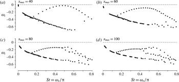
Eigenvalue spectra of a jet at
 $Re=1000$
,
 $S=0.5$
and
 $D/\unicode[STIX]{x1D703}_{0}=24.3$
, obtained in numerical domains of different length.

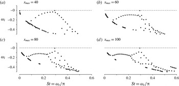
The eigenvalue spectrum for this setting is shown in figure 3, where different panels contain results obtained with different numerical box lengths
 $x_{max}$
between 40 and 100. The radial extent in all cases is
 $r_{max}=10$
. The dominant feature of the spectrum is an upper arching branch of eigenvalues, named the arc branch in the following. Eigenvalues are distributed along it with an even spacing in the real frequency. All eigenvalues are confined to the stable half-plane of
 $\unicode[STIX]{x1D714}$
, but in the case of the shortest box length,
 $x_{max}=40$
, the arc branch nearly crosses into the unstable domain. Clearly, convergence with respect to the box length
 $x_{max}$
is not achieved. This is consistent with the analysis of constant-density jets by Garnaud et al. (Reference Garnaud, Lesshafft, Schmid and Huerre2013a
), who argue that a further increase of
 $x_{max}$
is not guaranteed to ever lead to convergence. It seems unreasonable anyway to assume that the linear dynamics more than 100 radii downstream of the nozzle, in a hypothetical steady flow, should have any physical relevance.
A lower branch of densely packed eigenvalues is also observed. These modes have been discussed by Garnaud et al. (Reference Garnaud, Lesshafft, Schmid and Huerre2013a ), and they will not be investigated in more depth in this paper.
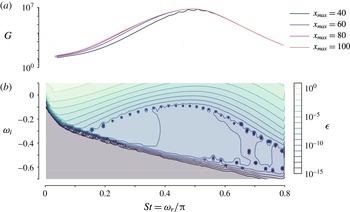
Forcing response of a jet at
 $Re=1000$
,
 $S=0.5$
and
 $D/\unicode[STIX]{x1D703}_{0}=24.3$
. (a) Optimal gain as a function of real forcing frequency. Different colours denote results obtained in numerical domains of different lengths, as indicated in the legend. (b) Pseudospectrum, represented as the inverse of the optimal gain for complex forcing frequencies,
 $\unicode[STIX]{x1D716}=\unicode[STIX]{x1D70E}^{-1}(\unicode[STIX]{x1D714})$
. The case
 $x_{max}=60$
is represented.

If the entire spectrum of a flow is stable, its dynamics in a noisy environment is determined by the response to external forcing. The linear frequency response of the present jet is represented in figure 4(a) by the optimal energy gain as a function of real forcing frequency (see § 2.5), as calculated in numerical domains of different length. The gain curve is clearly affected by domain truncation in the case of the shortest box length,
 $x_{max}=40$
, but all curves obtained with larger domains are seen to be in close agreement. The maximum gain is reached at
 $\unicode[STIX]{x1D714}_{r}=1.55$
, corresponding to a value of the Strouhal number based on the jet diameter
 $St=\unicode[STIX]{x1D714}_{r}/\unicode[STIX]{x03C0}=0.49$
. It is remarkable that the forced (exogenous) dynamics is well converged with respect to the box length, while the unforced (endogenous) dynamics is not. Note also that the maximum gain,
 $O(10^{7})$
, is very large compared to that of the constant-density setting,
 $O(10^{2})$
, investigated by Garnaud et al. (Reference Garnaud, Lesshafft, Schmid and Huerre2013b
), for the same value of the Reynolds number. The main difference between the two configurations lies in the choice of the base state, which in the case of Garnaud et al. (Reference Garnaud, Lesshafft, Schmid and Huerre2013b
) was a model mean flow with constant density.
The full pseudospectrum of the slowly developing jet is shown in figure 4(b). Two observations are pointed out: firstly, the arc branch is seen to align approximately with a pseudospectrum contour (here with a value of approximately
 $10^{-8}$
); secondly, the pseudospectrum variations below the arc branch are markedly different from those above the branch. Below the arc branch, the pseudospectrum indeed is nearly constant, compared to the strong variations in the upper part of the domain.
Pressure eigenfunction along
 $r=1$
for several modes of the arc branch for
 $S=0.5$
,
 $Re=1000$
and
 $D/\unicode[STIX]{x1D703}_{0}=24.3$
, with a numerical domain length
 $x_{max}=60$
.

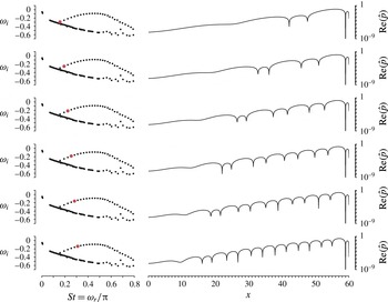
For a physical interpretation, eigenfunctions of the first six arc branch modes are represented in figure 5 by their pressure component along the nozzle lip line,
 $r=1$
, as a function of
 $x$
. Absolute real values
 $|\text{Re}(\hat{p})|$
are plotted in logarithmic scale, and the phase is adjusted such that
 $\text{Re}(\hat{p})$
is zero at
 $x=59$
in all cases. The eigenfunctions take the form of wavepackets; their particularity lies in the fact that each mode fits an integer number of wavelengths inside the numerical domain. Only the first six eigenfunctions are shown, but the same characteristic applies to all arc branch modes. The number of wavelengths increases steadily as one moves along the arc branch from low to higher real frequency values. This observation suggests that the arc branch is composed of box modes, similar to resonance modes in a pipe of finite length, a conjecture that deserves future investigation.
4 Analysis of a rapidly spreading pure helium jet
Eigenvalue spectra of a jet at
 $Re=360$
,
 $S=0.143$
and
 $D/\unicode[STIX]{x1D703}_{0}=24.3$
, obtained in numerical domains of different length.

A jet with parameters
 $S=0.143$
(pure helium),
 $D/\unicode[STIX]{x1D703}_{0}=24.3$
and
 $Re=360$
is considered next. The strong density contrast is certain to result in absolute instability close to the nozzle (Coenen & Sevilla Reference Coenen and Sevilla2012), and the low value of the Reynolds number leads to a fast viscous spreading of the jet base flow, as seen in figure 2(a).
The eigenvalue spectrum for this setting is shown in figure 6, where different panels again contain results obtained with different numerical box lengths
 $x_{max}$
between 40 and 100. The radial extent still is maintained at
 $r_{max}=10$
. One single eigenvalue
 $\unicode[STIX]{x1D714}=0.9197-0.0042\text{i}$
, very near marginal instability, is identically obtained (within
 $|\unicode[STIX]{x0394}\unicode[STIX]{x1D714}|=0.0015$
) independently of
 $x_{max}$
. This eigenmode, indeed the only one that seems to be converged with respect to box size, will be denoted here as the isolated mode.
An arc branch can be discerned, similar to the one described in § 3. In the spectrum of the shortest numerical box, figure 6(a), the eigenvalues along this branch are still evenly distributed. With larger box lengths, this regularity persists at low frequencies, but breaks down in the vicinity of the isolated mode. The pattern observed here resembles the ‘zipper phenomenon’, described by Heaton, Nichols & Schmid (Reference Heaton, Nichols and Schmid2009) and Nichols & Lele (Reference Nichols and Lele2011b ).
4.1 The isolated mode
The fact that the isolated mode is robust with respect to
 $x_{max}$
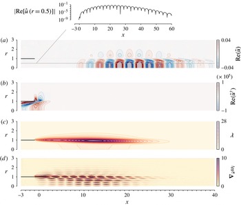
indicates that it must be quite distinct from the arc branch modes described earlier. A first characterisation of this mode is attempted by inspecting its spatial eigenfunction, shown in figure 7. Note that the results that are shown were obtained with
 $x_{max}=60$
, although for clarity only a fraction of the domain (up to
 $x=40$
and
 $r=3$
) is shown. The top frame (a) represents a snapshot of the axial velocity perturbation. Quite in contrast with the arc branch modes in figure 5, the region of significant eigenfunction amplitude is found to be well contained in the centre of the domain. This is seen even clearer when looking at the inset where the modulus of the perturbation values along a line
 $r=0.5$
is plotted in logarithmic scale. At the inflow and at the outflow boundaries, the perturbations are at least five orders of magnitude smaller than at their maximum location.
A numerical solution of the associated discrete adjoint eigenvalue problem retrieves the complex conjugate counterparts of the direct eigenvalues, as shown in figure 6, with high accuracy (arc branch and isolated mode). The adjoint eigenfunction of the isolated mode is displayed in figure 7(b). It is strongly localised around the nozzle edge, marking this region as being the most receptive to initial perturbations for triggering the direct eigenmode.
(a) Spatial structure of the eigenfunction of axial velocity
 $\hat{u}$
corresponding to the most unstable eigenmode for
 $S=0.143$
,
 $Re=360$
,
 $D/\unicode[STIX]{x1D703}_{0}=24.3$
, together with
 $|\text{Re}(\hat{u} )|$
along
 $r=0.5$
. (b) Spatial structure of the adjoint eigenmode associated with the direct mode shown in (a). (c) Structural sensitivity
 $\unicode[STIX]{x1D706}$
, as defined by (2.23). (d) Sensitivity
 $\unicode[STIX]{x1D735}_{\bar{\boldsymbol{u}}}\unicode[STIX]{x1D714}_{i}=(\unicode[STIX]{x1D735}_{\bar{u}}\unicode[STIX]{x1D714}_{i},\unicode[STIX]{x1D735}_{\bar{v}}\unicode[STIX]{x1D714}_{i})$
of the growth rate to modifications of the base flow.

Absolute value of the components of the structural sensitivity tensor
 $\unicode[STIX]{x1D64E}$
corresponding to the most unstable eigenmode for
 $S=0.143$
,
 $Re=360$
,
 $D/\unicode[STIX]{x1D703}_{0}=24.3$
.

Direct and adjoint eigenmodes may then be multiplied, according to (2.23), in order to estimate the flow region in which local feedback mechanisms contribute most to the existence of the global eigenmode. This quantity
 $\unicode[STIX]{x1D706}$
is represented in figure 7(c). A well-localised maximum is found around
 $x=13$
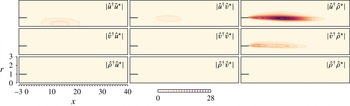
, concentrated near the lower part of the shear layer; the potential core is also highlighted. Comparing the individual components of the sensitivity tensor
 $\unicode[STIX]{x1D64E}$
, shown in figure 8, reveals that feedback proportional to the density perturbation
 $\unicode[STIX]{x1D70C}^{\prime }$
into the axial and – to a lesser degree – radial momentum equations forms the strongest contribution to changes in the eigenvalue. Note that it does not tell us whether these changes are stabilizing or destabilizing. From inspection of the stability equations (2.11)–(2.13) at zero Richardson number, we can thus draw the conclusion that the convection term
 $\bar{\boldsymbol{u}}\boldsymbol{\cdot }\unicode[STIX]{x1D735}\bar{\boldsymbol{u}}$
to which
 $\unicode[STIX]{x1D70C}^{\prime }$
is proportional plays a highly important role for the growth rate and frequency of the isolated eigenmode that is responsible for the self-sustained global oscillations in low-density jets. The fact that the feedback has a stronger effect in the axial momentum equation than in the radial momentum equation can easily be explained by remembering that the slenderness of this moderately large Reynolds number jet flow implies that
 $\bar{u}\gg \bar{v}$
and consequently
 $\bar{u}\unicode[STIX]{x2202}\bar{u}/\unicode[STIX]{x2202}x\gg \bar{u}\unicode[STIX]{x2202}\bar{v}/\unicode[STIX]{x2202}x$
.
It is tempting, but hardly pertinent, to try to relate the spatial distribution of the structural sensitivity to a supposed jet-column character of the eigenmode. The distinction between jet-column and shear layer modes is meaningful in the context of a local analysis. A physical examination of the active instability mechanisms in the isolated mode should ideally be based on the role of the baroclinic torque, following the local analysis of Lesshafft & Huerre (Reference Lesshafft and Huerre2007). However, it is not clear how the structural sensitivity could be exploited for such a discussion.
It is noted from figure 7 that the shapes of the direct and adjoint eigenmodes, as well as their pointwise product, compare well with the results of Qadri (Reference Qadri2014), shown in his figure 4.1. Recently, Qadri et al. (Reference Qadri, Chandler and Juniper2015) have analysed self-sustained oscillations in lifted diffusion flames. In their configuration, fuel with a density 7 times smaller than that of the ambient is injected at a Reynolds number, based on the present scales, of approximately 500, with a moderately steep velocity profile,
 $D/\unicode[STIX]{x1D703}_{0}=25$
. Given the similarities with the present set-up, it is not surprising that there are also many similarities between their ‘mode A’ and the isolated eigenmode under consideration here. For example, the structural sensitivity component with the strongest contribution in their work is that associated with changes in the mixture fraction feedback into the axial momentum equation (figure 6 of Qadri et al. (Reference Qadri, Chandler and Juniper2015)). Upstream of the diffusion flame, in the isothermal jet zone where the sensitivity of their mode A peaks, the mixture fraction is equivalent to the density, so that their strongest sensitivity component is in fact the analogue of
 $\hat{u} ^{\dagger }\hat{\unicode[STIX]{x1D70C}}^{\ast }$
in the present analysis, which has indeed been shown to be the strongest contributor to the structural sensitivity (figure 8). We would like to point out, however, that the low-density jet region in Qadri et al. (Reference Qadri, Chandler and Juniper2015) is bounded by a diffusion flame downstream, and is thus not a canonical jet configuration.
Figure 7(d) shows the sensitivity of the growth rate of the global mode to arbitrary modifications of the base flow. The magnitude
 $[(\unicode[STIX]{x1D735}_{\bar{u}}\unicode[STIX]{x1D714}_{i})^{2}+(\unicode[STIX]{x1D735}_{\bar{v}}\unicode[STIX]{x1D714}_{i})^{2}]^{1/2}$
is indicated by the colour, whereas the arrows indicate the direction
 $(\unicode[STIX]{x1D735}_{\bar{u}}\unicode[STIX]{x1D714}_{i},\unicode[STIX]{x1D735}_{\bar{v}}\unicode[STIX]{x1D714}_{i})$
in which the base flow has to be modified to achieve a positive increment in the growth rate, i.e. to destabilize the global mode. The results are in line with those observed by Tammisola (Reference Tammisola2012) for unconfined wake flows, i.e. a region of high sensitivity just downstream of the injector, followed by on oscillatory pattern in a region that stretches from approximately 5 to 20 radii downstream of the injector. This sensitivity measure can be further separated in two parts: the sensitivity to changes in the base flow advection and the sensitivity to changes in the energy extraction from base flow gradients (‘production’). It was found (not shown in the figure) that the contribution of the production part corresponds to the region of high sensitivity adjacent to the nozzle, while the advection part dominates in the second region of high sensitivity farther downstream. A change in the velocity profiles just downstream of the injector in the direction indicated by
 $(\unicode[STIX]{x1D735}_{\bar{u}}\unicode[STIX]{x1D714}_{i},\unicode[STIX]{x1D735}_{\bar{v}}\unicode[STIX]{x1D714}_{i})$
would cause a thinning of the shear layer, increasing the streamwise velocity gradient while bringing together the inflection points of the density and velocity profiles. From a local stability point of view (Lesshafft & Marquet Reference Lesshafft and Marquet2010; Coenen & Sevilla Reference Coenen and Sevilla2012), it is not surprising that such a change would cause a destabilisation of the flow.
If the isolated mode is not the result of non-local pressure feedback, which in the present setting could only arise from spurious effects at the outflow boundary, then it is expected to be linked to the presence of local absolute instability. According to previous studies, for instance Lesshafft et al. (Reference Lesshafft, Huerre and Sagaut2007), global instability in jets requires an absolutely unstable region of finite extent adjacent to the nozzle exit. To confirm the absolute character of the local instability near the nozzle in the present base flow, a local spatio-temporal stability analysis has been performed. To that aim, at each downstream position
 $x$
, the basic flow is assumed to be locally parallel, with radial profiles of velocity
 $\bar{\boldsymbol{u}}(r)=(\bar{u}(r),0)$
and density
 $\bar{\unicode[STIX]{x1D70C}}(r)$
; small perturbations are introduced as normal modes
 $[\hat{u} _{l}(r),\text{i}\hat{v}_{l}(r),\hat{p}_{l}(r),\hat{\unicode[STIX]{x1D70C}}_{l}(r)]\exp [\text{i}(kx-\unicode[STIX]{x1D714}t)]$
, with complex axial wavenumber
 $k=k_{r}+\text{i}k_{i}$
and complex angular frequency
 $\unicode[STIX]{x1D714}=\unicode[STIX]{x1D714}_{r}+\text{i}\unicode[STIX]{x1D714}_{i}$
. Here
 $k$
,
 $\unicode[STIX]{x1D714}$
, and
 $t$
are non-dimensionalised using
 $R^{\ast }$
and
 $U_{m}^{\ast }$
. Substitution of the normal modes into the equations of motion, linearised around the steady base flow, yields a system of ordinary differential equations that, together with appropriate boundary conditions, provides a generalised eigenvalue problem (see, for instance, Coenen & Sevilla Reference Coenen and Sevilla2012), to be interpreted as a dispersion relation
 $D(k,\unicode[STIX]{x1D714};Re,S,D/\unicode[STIX]{x1D703}_{0},\ldots ,\bar{u},\bar{v},\bar{p},\bar{\unicode[STIX]{x1D70C}})=0$
between
 $k$
and
 $\unicode[STIX]{x1D714}$
. Here we are concerned with the absolute or convective character of the instability. Therefore we need to find the spatio-temporal instability modes with zero group velocity, i.e. modes for which
 $\text{d}\unicode[STIX]{x1D714}/\text{d}k=0$
. The growth rate
 $\unicode[STIX]{x1D714}_{0,i}$
of these is called the absolute growth rate and determines whether the instability is convective,
 $\unicode[STIX]{x1D714}_{0,i}<0$
, or absolute,
 $\unicode[STIX]{x1D714}_{0,i}>0$
. The condition
 $\text{d}\unicode[STIX]{x1D714}/\text{d}k=0$
is equivalent to the existence of a double root, or saddle point, in the complex
 $k$
-plane,
 $\unicode[STIX]{x2202}D/\unicode[STIX]{x2202}k|_{k=k_{0}}=0$
. Among all the saddle points that may exist, only the one with the largest value of
 $\unicode[STIX]{x1D714}_{0,i}$
, while satisfying the Briggs–Bers criterion, determines the large-time impulse response of the flow (see, for instance, Huerre Reference Huerre, Batchelor, Moffatt and Worster2000, and references therein). The numerical method used to determine
 $(\unicode[STIX]{x1D714}_{0,i},k_{0,i})$
is described in Coenen & Sevilla (Reference Coenen and Sevilla2012).
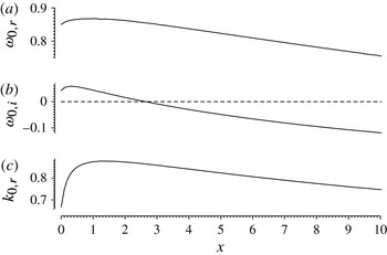
Figure 9 shows the streamwise variation of
 $\unicode[STIX]{x1D714}_{0,r}$
,
 $\unicode[STIX]{x1D714}_{0,i}$
, and
 $k_{0,r}$
. Absolute instability prevails over the interval
 $0\leqslant x\leqslant 2.6$
. Couairon & Chomaz (Reference Couairon and Chomaz1999) and Lesshafft et al. (Reference Lesshafft, Huerre, Sagaut and Terracol2006) showed that when an absolutely unstable region is bounded by the jet outlet, the length
 $x_{AC}$
of this region needs to be sufficiently large for the global mode to be triggered. Coenen & Sevilla (Reference Coenen and Sevilla2012) used the criterion
 $x_{AC}=C/\sqrt{\unicode[STIX]{x1D714}_{i}(x=0)}$
(Chomaz, Huerre & Redekopp Reference Chomaz, Huerre and Redekopp1988; Couairon & Chomaz Reference Couairon and Chomaz1999) that contains a free parameter
 $C$
. They found that
 $C=0.85$
gave good agreement with the experimental observations of Hallberg & Strykowski (Reference Hallberg and Strykowski2006). The same criterion would predict here that the length of the absolutely unstable region must be 4 radii. In figure 9 we can observe that for this globally marginally stable flow, this length is approximately 3 radii. From the spatially oscillating structure of the global mode of figure 7(a), we can also estimate a wavenumber
 $k=1.4$
, to be compared with the value
 $0.7\simeq k_{0,r}\simeq 0.9$
in the absolutely unstable region of figure 9(c). The frequency of the global mode for this case is
 $\unicode[STIX]{x1D714}_{r}=0.91$
, whereas the local stability analysis results in a frequency that ranges from 0.85 to 0.87. The discrepancies between the two analyses can be attributed to the rapid spatial development of the flow (see figure 2
a) that violates the parallel flow hypothesis on which the local analysis is based. An clear example of this was found recently by Moreno-Boza et al. (Reference Moreno-Boza, Coenen, Sevilla, Sanchez and Liñán2016) when studying buoyancy-driven flickering in diffusion flames.
Results of a local stability analysis for the case
 $S=0.143$
,
 $Re=360$
,
 $D/\unicode[STIX]{x1D703}_{0}=24.3$
.

As the current value
 $S=0.143$
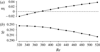
already represents the case of pure helium, in figure 10 the Reynolds number is varied in order to demonstrate its influence on the isolated eigenvalue. Indeed, the growth rate
 $\unicode[STIX]{x1D714}_{i}$
is found to increase steadily with the Reynolds number, crossing into the unstable half-plane before
 $Re=380$
, while the Strouhal number remains almost constant over the plotted interval of
 $Re$
.
Evolution of the isolated mode with the Reynolds number for a pure helium jet (
 $S=0.143$
) and
 $D/\unicode[STIX]{x1D703}_{0}=24.3$
.

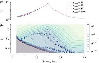
The pseudospectrum of the
 $Re=360$
helium jet is presented in figure 11 for a complete comparison with the
 $Re=1000$
case in the previous section. Most features are shared by both configurations, in particular the distinct variations of the energy gain in the regions above and below the arc branch. The response to forcing at real frequency is well converged in the case of the
 $Re=360$
jet at all
 $x_{max}$
settings. The most prominent difference with respect to the
 $Re=1000$
case is a sharp resonance peak in the energy gain near the frequency of the isolated mode. The gain remains finite, because the isolated mode is still slightly stable. The discussion of the arc branch provided in § 3 remains valid in all aspects in the present configuration.
Forcing response of a jet at
 $Re=360$
,
 $S=0.143$
and
 $D/\unicode[STIX]{x1D703}_{0}=24.3$
. (a) Optimal gain as a function of real forcing frequency. Different colours denote results obtained in numerical domains of different lengths, as indicated in the legend. (b) Pseudospectrum, computed as the inverse of the optimal gain for complex forcing frequencies. The case
 $x_{max}=60$
is represented.

4.2 Comparison with the experiment
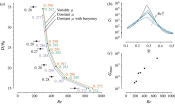
(a) Comparison with the experimental results of Hallberg & Strykowski (Reference Hallberg and Strykowski2006) for the onset of global instability in a pure
 $\text{He}$
jet (
 $S=0.143$
). The experimental results are indicated with solid squares and error bars, whereas the predictions based on the global mode analysis of the present work are indicated by the solid circles. The addition of gravitational effects in the analysis results in the transition points indicated by the solid triangles, and taking into account the variation of viscosity with composition results in the solid diamonds. The numbers next to the transition points indicate the Strouhal numbers corresponding to the oscillating mode of the jet. (b) Frequency response computed for conditions of the experimentally observed transition points. (c) The maximum optimal gain for the experimentally observed transition points.

The pure helium jet at
 $Re=360$
discussed in § 4 has been characterised as being nearly marginally stable. By tracking the values of the control parameters
 $Re$
and
 $D/\unicode[STIX]{x1D703}_{0}$
for which the growth rate of the isolated mode
 $\unicode[STIX]{x1D714}_{i}$
is zero, a neutral curve can be constructed. In figure 12(a), such neutral curves in the
 $Re{-}D/\unicode[STIX]{x1D703}_{0}$
plane are presented for pure helium jets (
 $S=0.143$
). The solid circles correspond to the results of the global mode analysis without taking into account buoyancy effects. To the left of the transition points the jet is globally stable (
 $\unicode[STIX]{x1D714}_{i}<0$
) whereas to the right it is globally unstable (
 $\unicode[STIX]{x1D714}_{i}>0$
). These results are compared with the experimental measurements of Hallberg & Strykowski (Reference Hallberg and Strykowski2006), indicated in figure 12(a) as squares with error bars. Care has been taken to convert the experimentally obtained critical Reynolds numbers, based on the centreline velocity, to Reynolds numbers based on the mean velocity. Fair agreement is found between the experimental and the linear neutral curves, but essentially the latter is shifted towards higher Reynolds numbers; in other words, the onset of global instability in the linear calculations is delayed with respect to the experimental observations.
Values next to the transition points in figure 12(a) indicate the Strouhal numbers near criticality. In the global mode calculations, the Strouhal number
 $St$
is directly given by the frequency
 $\unicode[STIX]{x1D714}_{r}$
of the marginally stable eigenmode, whereas in the experiments, it was obtained by measuring the frequency of the self-sustained oscillations under slightly supercritical conditions. It can be observed that the agreement between the two is rather good, with relative differences smaller than 10 %.
In an effort to explain the offset between the critical curve given by the stability analysis and the experimental evidence, we assessed the influence of buoyancy. Strictly speaking, while estimating the importance of the latter, the characteristic length scale that should be used in the construction of the Richardson number is not the radius
 $R^{\ast }$
, but the development length of the jet, of order
 $ReR^{\ast }$
. This modified Richardson number can be written as
 $Gr/Re$
. In the experiments of Hallberg & Strykowski (Reference Hallberg and Strykowski2006) the Grashof number for the pure helium jet (
 $S=0.143$
) is
 $Gr=138$
, and the marginal Reynolds numbers lie in the range 200–700. We can therefore expect that buoyancy has a non-negligible effect in the experiments. Recomputing the critical curve with the inclusion of the buoyancy term, with
 $Gr=138$
, we obtained the solid triangles of figure 12(a). Indeed, adding buoyancy destabilises the jet, and slightly improves the agreement with the experimental data. Nevertheless, its influence is not sufficiently strong to explain the offset between the stability analysis and the experiments.
A second physical aspect whose influence has been investigated is the variation of viscosity with composition. The viscosity of air is 11 % lower than that of helium, so that a small effect on the molecular transport can be expected, changing both the base flow and the stability properties. Figure 12(a) shows that there is indeed a small shift of the transition curve (solid diamonds). The variable viscosity is seen to have a slightly stabilising influence. This seems counterintuitive, as a lower viscosity in the flow field due to variations with the composition would result in an higher local effective Reynolds number, and would therefore be expected to destabilize the flow. Nevertheless, subtle changes in the base flow profiles may just as well counteract this, eventually causing a net stabilization. A more detailed study may be interesting in flows where variations of the viscosity are stronger, such as heated jets or diffusion flames.
In figure 12(b) we show the frequency response computed at the transition points of Hallberg & Strykowski (Reference Hallberg and Strykowski2006). Because these points are located to the left of the transition curve obtained with the global mode stability analysis, the jet is globally stable under these conditions. Nevertheless, the optimal gain is seen to be very high,
 $O(10^{3}{-}10^{6})$
, in a narrow band around the frequency associated with the global mode (see also the discussion of figure 11). This means that small perturbations that act as a forcing to the jet may suffer very strong amplifications that may sustain a nonlinear global oscillation of the jet at the frequency of maximum amplification. In an experiment this could cause a shift in the observed critical value of the bifurcation parameter. Applying this hypothesis to the present analysis would mean that, if both the incoming noise and the necessary amplification threshold to sustain a nonlinear oscillation were constant over all experimental conditions, the computed frequency response at the experimental transition points should have values that are of the same order of magnitude. Nevertheless, figure 12(b) shows that this is not the case here. In fact, the maximum gain is seen to be larger for the experimental conditions corresponding to higher Reynolds numbers (and lower
 $D/\unicode[STIX]{x1D703}_{0}$
). It must be mentioned that these results correspond to the optimal forcing, whose spatial structure varies from case to case, and might be very different from realistic noise present under experimental conditions. To rule out this variability the computations were repeated for a fixed spatial forcing distribution (a uniform distribution in the injection pipe), yielding similar results (not shown here) to the ones of figure 12(b), but with generally lower values of the gain.
Finally, it is worth mentioning that, as the sensitivity to base flow modifications of figure 7(d) shows, small changes in the region just downstream of the injector have a strong influence on the growth rate of the global instability. Although care has been taken to mimic the experimental set-up of Hallberg & Strykowski (Reference Hallberg and Strykowski2006), some details, such as the exact nozzle shape and the sharpness of the nozzle lip, are hard to account for, and may as well play a role in the discrepancy between experiment and linear theory.
5 Conclusions
The present work gives, for the first time, a detailed account of the linear global stability of low-density jets. By making use of the low Mach number approximation, all dynamic effects of density variations in the limit of zero Mach number are retained, while avoiding the numerically challenging necessity to resolve acoustic wave propagation.
We have found that when the spatial development of the jet flow is sufficiently fast (
 $Re=360$
and
 $S=0.143$
), an isolated eigenvalue dominates the global eigenvalue spectrum. This mode has been shown to arise from the presence of absolute instability in light jets, documented in numerous earlier studies (e.g. Monkewitz & Sohn Reference Monkewitz and Sohn1988; Lesshafft & Huerre Reference Lesshafft and Huerre2007; Coenen & Sevilla Reference Coenen and Sevilla2012). It is this mode that causes global instability in light jets at low Mach numbers. It has been found to converge without much effort in our numerical calculations, in particular with respect to the domain size. The structural sensitivity of this mode is concentrated in a confined region close to the nozzle; according to Giannetti & Luchini (Reference Giannetti and Luchini2007), it is sufficient to resolve this flow region in order to accurately compute the eigenvalue.
Unlike previous local stability analyses (e.g. Coenen & Sevilla Reference Coenen and Sevilla2012), in which the length of the absolutely unstable region that is necessary to trigger a global mode introduces an unknown parameter in the problem, the isolated global eigenmode is able the determine the critical conditions for the onset of global instability in terms of the governing flow parameters without any additional hypotheses. This has been employed to link the isolated mode to the supercritical Hopf bifurcation that was observed in the helium jet experiments by Hallberg & Strykowski (Reference Hallberg and Strykowski2006): the neutral curves for the onset of instability, in the experiments and in the present linear analysis match, within reasonable accuracy, and the predicted Strouhal numbers agree within ten per cent with the experimentally reported values at onset. The bifurcation in the experiments takes place in situations that are characterised as slightly subcritical in the linear framework. An additional destabilisation due to buoyancy effects has been demonstrated to be insufficient in order to explain this offset. Including the variation of viscosity with composition has been shown to have a small stabilising effect, and is thus also ruled out as an essential ingredient to explain the discrepancy. An inspection of the pseudospectrum however indicates that small perturbations may suffer a very strong amplification in the slightly stable regime. According to linear theory, experimental low-level noise might therefore be amplified and observed as sustained coherent wavepackets. A dedicated detailed study is required to assess this hypothesis, for example by comparing with direct numerical simulations with a controlled low-level forcing.
A second feature of the global eigenvalue spectra of low-density jets is a branch of eigenvalues, called the arc branch, that, when the spatial development of the jet flow is sufficiently slow (
 $Re=1000$
,
 $S=0.5$
) may dominate the spectrum, hindering the detection of the isolated mode. This arc branch is found to be highly sensitive to the numerical domain size, consistent with numerous existing studies of jets (Nichols & Lele Reference Nichols and Lele2011a
; Garnaud et al.
Reference Garnaud, Lesshafft, Schmid and Huerre2013a
) and boundary layers (Ehrenstein & Gallaire Reference Ehrenstein and Gallaire2005, Reference Ehrenstein and Gallaire2008; Åkervik et al.
Reference Åkervik, Ehrenstein, Gallaire and Henningson2008). The present results suggest, for the first time, that these eigenmodes are not only affected by domain truncation, but that their very existence is dependent on spurious feedback from the outflow boundary. Two observations support this conjecture: first, the arc branch aligns approximately with isocontours of the pseudospectrum, suggesting a link between a given level of exogenous energy input and the occurrence of arc branch modes; second, the associated eigenfunctions display an integer number of wavelengths between inflow and outflow, suggesting a resonance condition. A more detailed study to prove this conjecture is currently being carried out, but lies out of the scope of the present work.
Acknowledgements
L.L. acknowledges financial support from ANR under the Cool Jazz project and from DGA under contract LADX2331. W.C. and A.S. were supported by the Spanish MICINN under project DPI2014-59292-C3-1-P and DPI2015-71901-REDT.