1 Introduction
Variable-density flows are ubiquitous in technology and nature. For example, significant variations in fluid density are encountered in high-speed flight, combustion, multiphase flows and inertial confinement fusion. In nature, atmospheric and oceanic convection as well as astrophysical phenomena involve variable-density fluid dynamics.
Density variations in fluids can have different physical origins such as compressibility, thermal, compositional and phase inhomogeneity, chemical reactions and external energy sources and sinks. Primarily, there are two ways in which variations in the local density field interact with the local velocity field (Lele Reference Lele1994): inertial effects, in which spatial variations in density correspond to spatial variations in the local pressure-gradient-driven acceleration field, and dilatational effects, in which the Lagrangian variation in density corresponds to compression or expansion of the local Eulerian fluid element. These local interactions can significantly alter the global flow dynamics. An important example of inertial effects is the case of variable-density jets, where the jet to free-stream density ratio affects the global stability characteristics (Sreenivasan, Raghu & Kyle Reference Sreenivasan, Raghu and Kyle1989; Monkewitz et al.
Reference Monkewitz, Bechert, Barsikow and Lehmann1990) in free and transverse jets (Getsinger, Hendrickson & Karagozian Reference Getsinger, Hendrickson and Karagozian2012). Another example of an inertial effect is the case of interfacial instabilities associated with accelerated variable-density interfaces, such as Rayleigh–Taylor (Joly, Fontane & Chassaing Reference Joly, Fontane and Chassaing2005) and Richtmyer–Meshkov instabilities (Brouillette Reference Brouillette2002). The primary mechanism underlying these instabilities is baroclinic torque. The torque is produced by misalignment of independent thermodynamic quantities like pressure
 $p$
and density
 $\unicode[STIX]{x1D70C}$
or, equivalently, temperature and entropy, and is represented in the general form of the vorticity equation
 $$\begin{eqnarray}\frac{\unicode[STIX]{x2202}\unicode[STIX]{x1D74E}}{\unicode[STIX]{x2202}t}+\unicode[STIX]{x1D735}\times (\unicode[STIX]{x1D74E}\times \boldsymbol{v})=\frac{1}{\unicode[STIX]{x1D70C}^{2}}\unicode[STIX]{x1D735}\unicode[STIX]{x1D70C}\times \unicode[STIX]{x1D735}p+\unicode[STIX]{x1D735}\times \left(\frac{\unicode[STIX]{x1D735}\boldsymbol{\cdot }\unicode[STIX]{x1D748}}{\unicode[STIX]{x1D70C}}\right)+\unicode[STIX]{x1D735}\times \boldsymbol{F}^{b},\end{eqnarray}$$
where vorticity
 $\unicode[STIX]{x1D714}$
is the curl of velocity
 $v$
,
 $\unicode[STIX]{x1D748}$
is the viscous stress tensor and
 $\boldsymbol{F}^{b}$
is the non-conservative body force. In the framework of the Kovasznay decomposition of turbulent fluctuations (Kovasznay Reference Kovasznay1953), the interaction of acoustic and entropy modes produces vorticity modes via the baroclinic source term. This torque is also the primary vorticity source in shock–bubble (Ranjan, Oakley & Bonazza Reference Ranjan, Oakley and Bonazza2011) and shock–flame interactions (Thomas, Bambrey & Brown Reference Thomas, Bambrey and Brown2001). Baroclinic instability and associated turbulence are also observed in the form of midlatitude storms in the atmosphere (Pierrehumbert & Swanson Reference Pierrehumbert and Swanson1995) and mesoscale eddies in the ocean (Gill, Green & Simmons Reference Gill, Green and Simmons1974). In the atmosphere, the Earth’s rotation and differential heating produce vorticity, while in the oceans, horizontal density gradients are responsible. Secondary instabilities due to baroclinic torque are observed in two-dimensional Kelvin–Helmholtz billows of variable-density shear layers, as shown in the work of Reinaud, Joly & Chassaing (Reference Reinaud, Joly and Chassaing2000) and Fontane & Joly (Reference Fontane and Joly2008). Variable-density inertial effects are not restricted to instabilities in quiescent flow states, but are also present in fully turbulent flows. For example, the density ratio of the streams in a mixing layer affects the entrainment ratio and composition of molecularly mixed fluid in mixing layers (Frieler & Dimotakis Reference Frieler and Dimotakis1988; Miller, Bowman & Mungal Reference Miller, Bowman and Mungal1998). This is in addition to the reduction in growth rate and structural changes associated with increasing compressibility (Brown & Roshko Reference Brown and Roshko1974; Vreman, Sandham & Luo Reference Vreman, Sandham and Luo1996; Freund, Lele & Moin Reference Freund, Lele and Moin2000; Pantano & Sarkar Reference Pantano and Sarkar2002; Ferrer, Lehnasch & Mura Reference Ferrer, Lehnasch and Mura2017) and/or combustion-induced heat release. The composition of molecularly mixed fluid has direct implications in the case of reactive mixing. In the reacting case, dilatational and baroclinic effects associated with heat release also contribute to the vorticity dynamics. Similarly, high-speed turbulent boundary layers exhibit significant variable-density effects due to near-wall thermal gradients (Spina, Smits & Robinson Reference Spina, Smits and Robinson1994). This is reflected in the inertial transformations used to collapse the velocity profiles, such as the mean-density-based Van Driest transformation for adiabatic boundary layers (Van Driest Reference Van Driest1951) and mean-density-gradient-based transformations for non-adiabatic walls (Patel, Boersma & Pecnik Reference Patel, Boersma and Pecnik2016; Trettel & Larsson Reference Trettel and Larsson2016).
Simulations of technologically relevant variable-density turbulent flows require truncation of the spatio-temporal scales of the computed physical fields due to computational expense. Exclusion of information that represents a part of the physical system introduces the closure problem via the nonlinearity of the governing equations. For accurate simulations, the closure problem has to be addressed, whether the simulations compute the time-averaged fields, as in Reynolds-averaged Navier–Stokes (RANS), or the spatially filtered fields, as in large-eddy simulations (LES). This paper focuses on the closure problem that results from non-representation of small-scale density fluctuations in LES. The set of terms that require closure depends on the choice of the computed velocity field. For example, in the context of RANS, the choice of computed velocity variable can be either the time-averaged velocity or the density-weighted time-averaged velocity. The density-weighted averaging concept, also known as Favre averaging (Favre Reference Favre1969), is predominantly used. This method does not require closure of the mass conservation equation and retains the mathematical structure of the unclosed terms in a form that is structurally similar to their constant-density counterparts. Likewise, in LES, the resolved-scale velocity may be represented by the filtered velocity or Favre-filtered velocity. With the exception of the work of Yoshizawa (Reference Yoshizawa1986), Boersma & Lele (Reference Boersma and Lele1999) and Sun & Lu (Reference Sun and Lu2006), the Favre-filtered velocity is almost exclusively employed. The two velocity fields represent two different physical variables and their evolution is governed by different dynamics. An analogy may be drawn between the two resolved-scale velocities and the concept of mass velocity and momentum velocity introduced as bi-velocity hydrodynamics by Brenner (Reference Brenner2009).
Favre (Reference Favre1992) cited the importance of mass-averaged velocity for statistical analysis by stating that ‘the mean stream surfaces lose their physical meaning as the mean stream surfaces are crossed by the mean mass flux’ in the case of Reynolds-averaged velocity. It is important to consider Favre’s statement in the context of RANS and LES. While, in RANS, steady-state stream surfaces would be desirable for the description of the flow state, this may not hold true for LES filter volumes. The resolved-scale velocity represents the local value of the filtered Eulerian velocity field and may not necessarily represent the velocity of a frame of reference in which there is net zero subgrid-scale (SGS) mass diffusion through the LES filter volume. Therefore, in this paper, in addition to the Favre-filtered-velocity formulation, we also consider unclosed terms arising in filtered-velocity-based equations, which we refer to as the Reynolds-filtered formulation. We also note that the resolved-scale thermodynamic variables may be represented identically, Reynolds filtered or Favre filtered, irrespective of the choice of resolved-scale velocity. This is important as the representation of resolved-scale thermodynamic quantities is required to be consistent with the laws of thermodynamics (Favre Reference Favre1992; Chassaing Reference Chassaing1997). From the point of view of resolved-scale vorticity statistics, the Reynolds-filtered velocity is the preferred variable. This is because the curl of the Favre-filtered velocity does not mathematically equal the Favre-filtered vorticity. This holds more generally for the resolved-scale velocity-gradient tensor. Representation of the resolved-scale vorticity by a compound variable involving the density field can have implications during SGS modelling, where information from small velocity scales, close to the filter width, primarily guides the closure. In some previous work that uses the Favre-filtered-velocity formulation, the filtered velocity is algebraically estimated for closure even though it is not transported. This is discussed within an eddy viscosity framework by Germano (Reference Germano1996) and Germano et al. (Reference Germano, Abb, Arina and Bonaventura2014), and within the stretched-vortex model by Sidharth, Candler & Dimotakis (Reference Sidharth, Candler and Dimotakis2014). However, the equations based on the Reynolds-filtered velocity are not commonly used because they require closure of additional SGS terms in the momentum equation. This includes an unsteady time derivative term that can, in the case of strong density variations, be more significant than the SGS stress term (Chesnel et al. Reference Chesnel, Reveillon, Menard and Demoulin2011). In the present work, we will address this issue by deriving a new set of equations based on the Reynolds-filtered velocity, and that has a closure set with SGS terms that depend on double correlations. Although the equations are developed for LES, they are applicable to RANS due to the formal equivalence.
A review of the progress made in variable-density turbulence modelling is relevant as it helps to identify unclosed terms that are important in these classes of flows. Since spatio-temporal variations in fluid density can have different physical origins, a variety of modelling techniques exist, spanning low-speed variable-density turbulent mixing to high-speed turbulent flows and combustion. Reynolds-averaged Navier–Stokes modelling for variable-density turbulence has been a research field for several decades. Chassaing (Reference Chassaing2001) and Chassaing et al. (Reference Chassaing, Antonia, Anselmet, Joly and Sarkar2013) have provided a comprehensive review of variable-density modelling in RANS closure schemes. In first-order closures, variable-density effects in the turbulent kinetic energy and dissipation
 $k{-}\unicode[STIX]{x1D716}$
framework have been extensively studied. Important variable-density terms investigated are the turbulent mass flux (Ristorcelli Reference Ristorcelli1993), the pressure dilatation (Sarkar Reference Sarkar1992) and the dilatational dissipation (Zeman Reference Zeman1990). Moreover, terms associated with baroclinic torque and compression in the solenoidal dissipation rate equation have received interest (Sinha & Candler Reference Sinha and Candler2003; Kreuzinger, Friedrich & Gatski Reference Kreuzinger, Friedrich and Gatski2006). Some modelling techniques estimate the variance of density (Taulbee & VanOsdol Reference Taulbee and Vanosdol1991; Banerjee, Gore & Andrews Reference Banerjee, Gore and Andrews2010) and pressure (Zeman Reference Zeman1991). Within second-order closures, density fluctuation correlations have been analysed in the work of Shih, Lumley & Janicka (Reference Shih, Lumley and Janicka1987), Chassaing, Harran & Joly (Reference Chassaing, Harran and Joly1994), Schwarzkopf et al. (Reference Schwarzkopf, Livescu, Gore, Rauenzahn and Ristorcelli2011) and Yoshizawa, Matsuo & Mizobuchi (Reference Yoshizawa, Matsuo and Mizobuchi2013). Pressure–strain (Adumitroaie, Ristorcelli & Taulbee Reference Adumitroaie, Ristorcelli and Taulbee1999) and pressure–acceleration–mass-flux terms (Lindstedt & Vaos Reference Lindstedt and Vaos1999) have been shown to be important for closure in second-order moment equations. It is important to note that in both first-order and second-order modelling, the Favre-averaged velocity is usually the solution variable. Shih et al. (Reference Shih, Lumley and Janicka1987) investigated the evolution of non-density-averaged velocity in a variable-density mixing layer, but used a constant-density approximation for the turbulent pressure–acceleration term appearing in the equation for the mean velocity. In the class of algebraic second-order closures, an explicit algebraic stress model for compressible variable-density turbulent flows has been proposed (Grigoriev et al.
Reference Grigoriev, Wallin, Brethouwer and Johansson2015), where the effect of density–velocity correlations on turbulence is accounted for. The authors in this work state their preference for Reynolds averaging over Favre averaging due to turbulent dissipation being a function of the fluctuating velocity field, and not the density-averaged fluctuating velocity. Similarly, in the class of stochastic methods for turbulent flow simulation, variable-density effects such as differential acceleration have been included in the work of Bakosi & Ristorcelli (Reference Bakosi and Ristorcelli2011).
A significant effort to understand variable-density and dilatational effects in turbulence has been carried out for turbulent premixed flames (Lipatnikov & Chomiak Reference Lipatnikov and Chomiak2010; Robin, Mura & Champion Reference Robin, Mura and Champion2011; Sabelnikov & Lipatnikov Reference Sabelnikov and Lipatnikov2017). For example, Libby & Bray (Reference Libby and Bray1977) have pointed out that modelling of variable-density effects in turbulent flames is important and that there can be large differences between the Favre-averaged and Reynolds-averaged scalars and velocities in the flame zone. Moreover, assumptions such as neglecting third-order covariances can lead to inconsistent results. They also find that the Favre-averaged turbulent kinetic-energy production due to the pressure–acceleration–mass-flux term can override the suppression due to dilatation and cause countergradient turbulent diffusion of scalar concentration (Bilger Reference Bilger1976; Bray et al. Reference Bray, Libby, Masuya and Moss1981; Libby & Bray Reference Libby and Bray1981). The authors state that their results ‘constitute a warning as to the dangers of carrying over the empiricism developed in constant-density flows to variable-density flows in general and to turbulent reacting flows with significant heat release in particular’. Countergradient diffusion of scalars is more generally a variable-density effect in turbulence and has also been observed in inert helium–air mixing (LaRue & Libby Reference LaRue and Libby1977). Variable-density effects in turbulent flames have also been discussed extensively by Chomiak & Nisbet (Reference Chomiak and Nisbet1995). It must be noted, however, that the major focus of RANS analysis has been restricted to variable-density effects on the transport of second-order turbulent quantities. With regard to LES, there have been efforts to understand the role of filtered velocity and Favre-filtered velocity in turbulent flame dynamics. Chakraborty et al. (Reference Chakraborty, Wang, Konstantinou and Klein2017) showed that the difference between the orientation of the vorticity vector obtained from the filtered velocity and the Favre-filtered velocity in planar turbulent flames can be large. Serra et al. (Reference Serra, Robin, Mura and Champion2014) accounted for the difference between the Favre-filtered scalar and the filtered scalar using the SGS specific volume flux, similarly to the approach presented in Sidharth et al. (Reference Sidharth, Candler and Dimotakis2014). The concept of countergradient diffusion due to variable-density effects is observed in LES as well, but with different physical connotations (Klein et al. Reference Klein, Kasten, Gao and Chakraborty2015).
We focus on the variable-density SGS terms that appear in the resolved-scale momentum equation as opposed to terms that appear in the transport equations of SGS terms. The terms under consideration are listed in § 2, where we review the filtered compressible Navier–Stokes equations in the Favre-filtered and Reynolds-filtered formulations. A new form of the Reynolds-filtered governing equations is derived using the transport equations of SGS mass flux and SGS kinetic energy. This form of the governing equations does not contain unsteady unclosed terms. Flow fields from direct numerical simulations of single-fluid decaying isotropic turbulence with dynamically significant dilatational and inertial variable-density effects are used for the explicit evaluation of the SGS terms. The set-up of the direct numerical simulations, and results from the SGS analysis are discussed in §§ 3 and 4.
2 Filtered Navier–Stokes equations
Let us first review the formalism for filtering the Navier–Stokes equations and revisit the resulting governing equations. A spatio-temporal linear filter for a flow realization with
 $\boldsymbol{x}=x_{i}$
may be defined as
 $$\begin{eqnarray}\overline{f(\boldsymbol{x},t)}=\int G_{\unicode[STIX]{x1D6E5}_{x},\unicode[STIX]{x1D6E5}_{t}}(\boldsymbol{x}-\boldsymbol{x}^{\prime },t-t^{\prime })f(\boldsymbol{x}^{\prime },t)\,\text{d}^{3}\boldsymbol{x}^{\prime }\,\text{d}t^{\prime },\end{eqnarray}$$
where
 $G_{\unicode[STIX]{x1D6E5}_{x},\unicode[STIX]{x1D6E5}_{t}}$
is the convolution kernel with an associated filter length scale
 $\unicode[STIX]{x1D6E5}_{x}$
and a filter time scale
 $\unicode[STIX]{x1D6E5}_{t}$
, satisfying
 $$\begin{eqnarray}\int G_{\unicode[STIX]{x1D6E5}_{x},\unicode[STIX]{x1D6E5}_{t}}(\boldsymbol{x}-\boldsymbol{x}^{\prime })\,\text{d}^{3}\boldsymbol{x}^{\prime }\,\text{d}t^{\prime }=1.\end{eqnarray}$$
For LES, filters are spatial and no temporal filtering is considered in this paper. It must be noted that the continuous filter is independent of the filter associated with the discrete solution field and the discrete differential operators used for numerical computation. We assume that the continuous filter is homogeneous and therefore commutes with the continuous differential operator. The governing equations for filtered mass, momentum and energy are obtained from the filtered Navier–Stokes equations,
 $$\begin{eqnarray}\frac{\unicode[STIX]{x2202}}{\unicode[STIX]{x2202}t}\left(\begin{array}{@{}c@{}}\bar{\unicode[STIX]{x1D70C}}\\ \overline{\unicode[STIX]{x1D70C}u_{i}}\\ \frac{1}{2}\overline{\unicode[STIX]{x1D70C}u_{k}u_{k}}+\bar{E}_{\mathit{int}}\end{array}\right)+\frac{\unicode[STIX]{x2202}}{\unicode[STIX]{x2202}x_{j}}\left(\begin{array}{@{}c@{}}\overline{\unicode[STIX]{x1D70C}u_{j}}\\ \overline{\unicode[STIX]{x1D70C}u_{i}u_{j}}+\bar{p}\unicode[STIX]{x1D6FF}_{ij}\\ \frac{1}{2}\overline{\unicode[STIX]{x1D70C}u_{k}u_{k}}+\overline{E_{\mathit{int}}u_{j}}+\overline{pu_{j}}\\ \end{array}\right)=\left(\begin{array}{@{}c@{}}0\\ \bar{\unicode[STIX]{x1D70E}}_{\unicode[STIX]{x1D70C}u_{i}}\\ \bar{\unicode[STIX]{x1D70E}}_{E}\end{array}\right).\end{eqnarray}$$
Here,
 $E_{\mathit{int}}$
represents the internal energy per unit volume. The terms
 $\unicode[STIX]{x1D70E}_{\unicode[STIX]{x1D70C}u_{i}}$
and
 $\unicode[STIX]{x1D70E}_{E}$
correspond to diffusive molecular transport in the momentum and the energy equations respectively. In the present analysis, the resolved-scale and SGS terms that arise from the expressions for
 $\bar{\unicode[STIX]{x1D70E}}_{\unicode[STIX]{x1D70C}u_{i}}$
and
 $\bar{\unicode[STIX]{x1D70E}}_{E}$
are not expanded.
2.1 Favre-filtered velocity formulation
In the Favre-filtered velocity formulation, the filtered Navier–Stokes equations for variable-density flows are written in a form that uses the density-weighted filtered velocity as the resolved-scale velocity,
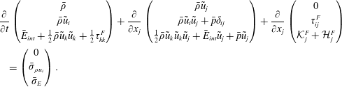 $$\begin{eqnarray}\displaystyle & & \displaystyle \frac{\unicode[STIX]{x2202}}{\unicode[STIX]{x2202}t}\left(\begin{array}{@{}c@{}}\bar{\unicode[STIX]{x1D70C}}\\ \bar{\unicode[STIX]{x1D70C}}\tilde{u} _{i}\\ \bar{E}_{\mathit{int}}+\frac{1}{2}\bar{\unicode[STIX]{x1D70C}}\tilde{u} _{k}\tilde{u} _{k}+\frac{1}{2}\unicode[STIX]{x1D70F}_{kk}^{\mathit{F}}\end{array}\right)+\frac{\unicode[STIX]{x2202}}{\unicode[STIX]{x2202}x_{j}}\left(\begin{array}{@{}c@{}}\bar{\unicode[STIX]{x1D70C}}\tilde{u} _{j}\\ \bar{\unicode[STIX]{x1D70C}}\tilde{u} _{i}\tilde{u} _{j}+\bar{p}\unicode[STIX]{x1D6FF}_{ij}\\ \frac{1}{2}\bar{\unicode[STIX]{x1D70C}}\tilde{u} _{k}\tilde{u} _{k}\tilde{u} _{j}+\bar{E}_{\mathit{int}}\tilde{u} _{j}+\bar{p}\tilde{u} _{j}\end{array}\right)+\frac{\unicode[STIX]{x2202}}{\unicode[STIX]{x2202}x_{j}}\left(\begin{array}{@{}c@{}}0\\ \unicode[STIX]{x1D70F}_{ij}^{\mathit{F}}\\ {\mathcal{K}}_{j}^{\mathit{F}}+{\mathcal{H}}_{j}^{\mathit{F}}\end{array}\right)\nonumber\\ \displaystyle & & \displaystyle \quad =\left(\begin{array}{@{}c@{}}0\\ \bar{\unicode[STIX]{x1D70E}}_{\unicode[STIX]{x1D70C}u_{i}}\\ \bar{\unicode[STIX]{x1D70E}}_{E}\end{array}\right).\end{eqnarray}$$
A Favre-filtered quantity is denoted by
 $$\begin{eqnarray}\tilde{f}=\frac{\overline{\unicode[STIX]{x1D70C}f}}{\bar{\unicode[STIX]{x1D70C}}}.\end{eqnarray}$$
The resolved-scale velocity,
 $\tilde{u} _{i}$
, is therefore obtained from the filtered momentum and the filtered density. The SGS terms in this formulation are the SGS stress tensor
 $\unicode[STIX]{x1D70F}_{ij}^{\mathit{F}}$
, the SGS kinetic-energy flux
 ${\mathcal{K}}_{j}^{\mathit{F}}$
and the SGS enthalpy flux
 ${\mathcal{H}}_{j}^{\mathit{F}}$
,
 $$\begin{eqnarray}\unicode[STIX]{x1D70F}_{ij}^{\mathit{F}}=\overline{\unicode[STIX]{x1D70C}u_{i}u_{j}}-\bar{\unicode[STIX]{x1D70C}}\tilde{u} _{i}\tilde{u} _{j},\quad {\mathcal{K}}_{j}^{\mathit{F}}=\overline{\unicode[STIX]{x1D70C}u_{k}u_{k}u_{j}}-\bar{\unicode[STIX]{x1D70C}}\tilde{u} _{k}\tilde{u} _{k}\tilde{u} _{j},\quad {\mathcal{H}}_{j}^{\mathit{F}}=\overline{(E_{\mathit{int}}+p)u_{j}}-(\bar{E}_{\mathit{int}}+\bar{p})\tilde{u} _{j}.\end{eqnarray}$$
The filtered convective stress
 $\overline{\unicode[STIX]{x1D70C}u_{i}u_{j}}$
is equivalent to the Favre-filtered specific stress
 $\bar{\unicode[STIX]{x1D70C}}\widetilde{u_{i}u_{j}}$
. The expression for the SGS stress,
 $\unicode[STIX]{x1D70F}_{ij}^{\mathit{F}}=\bar{\unicode[STIX]{x1D70C}}(\widetilde{u_{i}u_{j}}-\tilde{u} _{i}\tilde{u} _{j})$
, appears as a variable-density analogue of the constant-density specific stress tensor
 $\overline{u_{i}u_{j}}-\bar{u}_{i}\bar{u}_{j}$
.
The variable-density SGS contribution to the momentum equation can be written explicitly if we represent the SGS terms using central moments (Germano Reference Germano1992). Let us denote the central moments under the filter operator as
 $$\begin{eqnarray}\displaystyle & {\mathcal{T}}[a,b]=\overline{ab}-\bar{a}\bar{b}, & \displaystyle\end{eqnarray}$$
 $$\begin{eqnarray}\displaystyle & {\mathcal{T}}[a,b,c]=\overline{abc}-\bar{a}{\mathcal{T}}[b,c]-\bar{b}{\mathcal{T}}[a,c]-\bar{c}{\mathcal{T}}[a,b]-\bar{a}\bar{b}\bar{c}, & \displaystyle\end{eqnarray}$$
where
 $a$
,
 $b$
and
 $c$
are field variables. The SGS stress tensor can then be expressed as
 $$\begin{eqnarray}\displaystyle \unicode[STIX]{x1D70F}_{ij}^{\mathit{F}}=\bar{\unicode[STIX]{x1D70C}}(\widetilde{u_{i}u_{j}}-\tilde{u} _{i}\tilde{u} _{j})=\bar{\unicode[STIX]{x1D70C}}{\mathcal{T}}[u_{i},u_{j}]+{\mathcal{T}}[\unicode[STIX]{x1D70C},u_{i},u_{j}]-\frac{1}{\bar{\unicode[STIX]{x1D70C}}}{\mathcal{T}}[\unicode[STIX]{x1D70C},u_{i}]{\mathcal{T}}[\unicode[STIX]{x1D70C},u_{j}]. & & \displaystyle\end{eqnarray}$$
Equation (2.9) (Germano et al.
Reference Germano, Abb, Arina and Bonaventura2014) shows that the SGS stress tensor in either formulation involves three unclosed terms: the SGS specific stress tensor
 ${\mathcal{T}}[u_{i},u_{j}]$
, the SGS mass flux
 ${\mathcal{M}}_{i}={\mathcal{T}}[\unicode[STIX]{x1D70C},u_{i}]$
and the SGS trivariate moment
 ${\mathcal{T}}[\unicode[STIX]{x1D70C},u_{i},u_{j}]$
. Although absent in the mass conservation equation, the SGS mass flux
 ${\mathcal{M}}_{i}$
affects the Favre-filtered velocity SGS stress
 $\unicode[STIX]{x1D70F}_{ij}^{\mathit{F}}$
. The SGS trivariate moment also appears when the momentum
 $\mathfrak{p}_{i}=\unicode[STIX]{x1D70C}u_{i}$
is used as the variable of interest,
 $$\begin{eqnarray}\unicode[STIX]{x1D70F}_{ij}^{\mathit{F}}={\mathcal{T}}\left[\mathfrak{p}_{i},\mathfrak{p}_{j},\frac{1}{\unicode[STIX]{x1D70C}}\right]+\overline{\frac{1}{\unicode[STIX]{x1D70C}}}{\mathcal{T}}[\mathfrak{p}_{i},\mathfrak{p}_{j}]+\bar{\mathfrak{p}}_{i}{\mathcal{T}}\left[\mathfrak{p}_{j},\frac{1}{\unicode[STIX]{x1D70C}}\right]+\bar{\mathfrak{p}}_{j}{\mathcal{T}}\left[\mathfrak{p}_{i},\frac{1}{\unicode[STIX]{x1D70C}}\right]-\frac{\bar{\mathfrak{p}}_{i}\bar{\mathfrak{p}}_{j}}{\bar{\unicode[STIX]{x1D70C}}}{\mathcal{T}}\left[\unicode[STIX]{x1D70C},\frac{1}{\unicode[STIX]{x1D70C}}\right].\end{eqnarray}$$
Similarly, the SGS term
 ${\mathcal{K}}_{j}^{\mathit{F}}$
appearing in the filtered total energy equation can be shown to consist of a fourth-order-moment SGS term.
2.2 Reynolds-filtered velocity formulation
Now, let us represent the filtered Navier–Stokes equations using the filtered velocity. In this formulation, the equations are
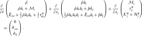 $$\begin{eqnarray}\displaystyle & & \displaystyle \frac{\unicode[STIX]{x2202}}{\unicode[STIX]{x2202}t}\left(\begin{array}{@{}c@{}}\bar{\unicode[STIX]{x1D70C}}\\ \bar{\unicode[STIX]{x1D70C}}\bar{u}_{i}+{\mathcal{M}}_{i}\\ \bar{E}_{\mathit{int}}+\frac{1}{2}\bar{\unicode[STIX]{x1D70C}}\bar{u}_{k}\bar{u}_{k}+\frac{1}{2}\unicode[STIX]{x1D70F}_{kk}^{\mathit{R}}\end{array}\right)+\frac{\unicode[STIX]{x2202}}{\unicode[STIX]{x2202}x_{j}}\left(\begin{array}{@{}c@{}}\bar{\unicode[STIX]{x1D70C}}\bar{u}_{j}\\ \bar{\unicode[STIX]{x1D70C}}\bar{u}_{i}\bar{u}_{j}+\bar{p}\unicode[STIX]{x1D6FF}_{ij}\\ \frac{1}{2}\bar{\unicode[STIX]{x1D70C}}\bar{u}_{k}\bar{u}_{k}\bar{u}_{j}+\bar{E}_{\mathit{int}}\bar{u}_{j}+\bar{p}\bar{u}_{j}\end{array}\right)+\frac{\unicode[STIX]{x2202}}{\unicode[STIX]{x2202}x_{j}}\left(\begin{array}{@{}c@{}}{\mathcal{M}}_{j}\\ \unicode[STIX]{x1D70F}_{ij}^{\mathit{R}}\\ {\mathcal{K}}_{j}^{\mathit{R}}+{\mathcal{H}}_{j}^{\mathit{R}}\end{array}\right)\nonumber\\ \displaystyle & & \displaystyle \quad =\left(\begin{array}{@{}c@{}}0\\ \bar{\unicode[STIX]{x1D70E}}_{\unicode[STIX]{x1D70C}u_{i}}\\ \bar{\unicode[STIX]{x1D70E}}_{E}\end{array}\right).\end{eqnarray}$$
The SGS terms with the superscript ‘
 $\mathit{R}$
’ denote the same SGS terms as in the
 $\tilde{u} _{i}$
formulation, but with
 $\bar{u}_{i}$
as the resolved-scale velocity. Here,
 $$\begin{eqnarray}\left.\begin{array}{@{}c@{}}{\mathcal{M}}_{i}=\overline{\unicode[STIX]{x1D70C}u_{i}}-\bar{\unicode[STIX]{x1D70C}}\bar{u}_{i},\quad \unicode[STIX]{x1D70F}_{ij}^{\mathit{R}}=\overline{\unicode[STIX]{x1D70C}u_{i}u_{j}}-\bar{\unicode[STIX]{x1D70C}}\bar{u}_{i}\bar{u}_{j},\\ {\mathcal{K}}_{j}^{\mathit{R}}=\overline{\unicode[STIX]{x1D70C}u_{k}u_{k}u_{j}}-\bar{\unicode[STIX]{x1D70C}}\bar{u}_{k}\bar{u}_{k}\bar{u}_{j},\quad {\mathcal{H}}_{j}^{\mathit{R}}=\overline{(E_{\mathit{int}}+p)u_{j}}-(\bar{E}_{\mathit{int}}+\bar{p})\bar{u}_{j}.\end{array}\right\}\end{eqnarray}$$
The additional SGS quantity
 ${\mathcal{M}}_{i}$
is the SGS mass flux and represents the spatial correlation of density with velocity under the filter operator. It is a measure of the difference between the quantity
 $\bar{\unicode[STIX]{x1D70C}}\bar{u}_{i}$
and the filtered momentum. With the use of central moments, the SGS stress in this formulation can be written as
 $$\begin{eqnarray}\displaystyle \unicode[STIX]{x1D70F}_{ij}^{\mathit{R}}=\overline{\unicode[STIX]{x1D70C}u_{i}u_{j}}-\bar{\unicode[STIX]{x1D70C}}\bar{u}_{i}\bar{u}_{j}=\bar{\unicode[STIX]{x1D70C}}{\mathcal{T}}[u_{i},u_{j}]+{\mathcal{T}}[\unicode[STIX]{x1D70C},u_{i},u_{j}]+\bar{u}_{i}{\mathcal{T}}[\unicode[STIX]{x1D70C},u_{j}]+\bar{u}_{j}{\mathcal{T}}[\unicode[STIX]{x1D70C},u_{i}]. & & \displaystyle\end{eqnarray}$$
We observe that the term
 $\unicode[STIX]{x1D70F}_{ij}^{\mathit{R}}$
, like
 $\unicode[STIX]{x1D70F}_{ij}^{\mathit{F}}$
, consists of the SGS specific stress, the SGS trivariate moment term and the SGS mass flux term. However, the resolved-scale momentum equation in this formulation also includes the rate of change of SGS mass flux.
In order to understand the unclosed time derivative, we examine the differences between
 $\bar{u}_{i}$
and
 $\tilde{u} _{i}$
by comparing their respective inviscid transport equations. The governing equation for the Favre-filtered velocity is obtained using the transport equations for the filtered momentum and filtered density. The equation for the filtered velocity is obtained by filtering the transport equation for the velocity. If we compare the two transport equations, it is seen that in the equation for
 $\bar{u}_{i}$
, there exist SGS terms other than the SGS specific stress
 ${\mathcal{T}}[u_{i},u_{j}]=\overline{u_{i}u_{j}}-\bar{u}_{i}\bar{u}_{j}$
,
 $$\begin{eqnarray}\displaystyle & \displaystyle {\displaystyle \frac{\unicode[STIX]{x2202}\tilde{u} _{i}}{\unicode[STIX]{x2202}t}}+\tilde{u} _{j}{\displaystyle \frac{\unicode[STIX]{x2202}\tilde{u} _{i}}{\unicode[STIX]{x2202}x_{j}}}+\frac{1}{\bar{\unicode[STIX]{x1D70C}}}{\displaystyle \frac{\unicode[STIX]{x2202}\bar{p}}{\unicode[STIX]{x2202}x_{i}}}+\frac{1}{\bar{\unicode[STIX]{x1D70C}}}{\displaystyle \frac{\unicode[STIX]{x2202}\bar{\unicode[STIX]{x1D70C}}(\widetilde{u_{i}u_{j}}-\tilde{u} _{i}\tilde{u} _{j})}{\unicode[STIX]{x2202}x_{j}}}=0, & \displaystyle\end{eqnarray}$$
 $$\begin{eqnarray}\displaystyle & \displaystyle {\displaystyle \frac{\unicode[STIX]{x2202}\bar{u}_{i}}{\unicode[STIX]{x2202}t}}+\bar{u}_{j}{\displaystyle \frac{\unicode[STIX]{x2202}\bar{u}_{i}}{\unicode[STIX]{x2202}x_{j}}}+\frac{1}{\bar{\unicode[STIX]{x1D70C}}}{\displaystyle \frac{\unicode[STIX]{x2202}\bar{p}}{\unicode[STIX]{x2202}x_{i}}}+{\displaystyle \frac{\unicode[STIX]{x2202}(\overline{u_{i}u_{j}}-\bar{u}_{i}\bar{u}_{j})}{\unicode[STIX]{x2202}x_{j}}}-{\mathcal{T}}\left[u_{i},{\displaystyle \frac{\unicode[STIX]{x2202}u_{j}}{\unicode[STIX]{x2202}x_{j}}}\right]-\frac{1}{\bar{\unicode[STIX]{x1D70C}}}{\mathcal{T}}\left[\unicode[STIX]{x1D70C},\frac{1}{\unicode[STIX]{x1D70C}}{\displaystyle \frac{\unicode[STIX]{x2202}p}{\unicode[STIX]{x2202}x_{i}}}\right]=0.\quad & \displaystyle\end{eqnarray}$$
These additional SGS terms are associated with dilatation,
 $\unicode[STIX]{x1D735}\boldsymbol{\cdot }u$
, and pressure–acceleration,
 $\unicode[STIX]{x1D735}p/\unicode[STIX]{x1D70C}$
. This is due to the non-conservative nature of velocity in the presence of variable-density effects.
The transport equations for
 $\tilde{u} _{i}$
(2.14) and
 $\bar{u}_{i}$
(2.15), with the filtered density equation, can be used to derive the transport equation for the SGS mass flux
 ${\mathcal{M}}_{i}$
,
 $$\begin{eqnarray}\displaystyle {\displaystyle \frac{\unicode[STIX]{x2202}{\mathcal{M}}_{i}}{\unicode[STIX]{x2202}t}} & = & \displaystyle {\displaystyle \frac{\unicode[STIX]{x2202}(\overline{\unicode[STIX]{x1D70C}u_{i}}-\bar{\unicode[STIX]{x1D70C}}\bar{u}_{i})}{\unicode[STIX]{x2202}t}}\nonumber\\ \displaystyle & = & \displaystyle -{\displaystyle \frac{\unicode[STIX]{x2202}\overline{\unicode[STIX]{x1D70C}u_{i}u_{j}}}{\unicode[STIX]{x2202}x_{j}}}+\bar{u}_{i}{\displaystyle \frac{\unicode[STIX]{x2202}{\mathcal{M}}_{j}}{\unicode[STIX]{x2202}x_{j}}}+{\displaystyle \frac{\unicode[STIX]{x2202}\bar{\unicode[STIX]{x1D70C}}\bar{u}_{i}\bar{u}_{j}}{\unicode[STIX]{x2202}x_{j}}}+\bar{\unicode[STIX]{x1D70C}}{\displaystyle \frac{\unicode[STIX]{x2202}{\mathcal{T}}[u_{i},u_{j}]}{\unicode[STIX]{x2202}x_{j}}}-\bar{\unicode[STIX]{x1D70C}}{\mathcal{T}}\left[u_{i},{\displaystyle \frac{\unicode[STIX]{x2202}u_{j}}{\unicode[STIX]{x2202}x_{j}}}\right]-{\mathcal{T}}\left[\unicode[STIX]{x1D70C},\frac{1}{\unicode[STIX]{x1D70C}}{\displaystyle \frac{\unicode[STIX]{x2202}p}{\unicode[STIX]{x2202}x_{i}}}\right].\nonumber\\ \displaystyle & & \displaystyle\end{eqnarray}$$
For the sake of clarity, we do not consider terms corresponding to viscous molecular transport and work with the inviscid transport equations; inclusion of the viscous transport term is straightforward and produces an additional term,
 ${\mathcal{T}}[\unicode[STIX]{x1D70C},\unicode[STIX]{x1D70E}_{\unicode[STIX]{x1D70C}u_{i}}/\unicode[STIX]{x1D70C}]$
, in (2.16). We note that the filtered momentum equation is a composite equation transporting two physical variables,
 $\bar{u}_{i}$
and
 ${\mathcal{M}}_{i}$
. This implies that a part of the SGS term
 $\unicode[STIX]{x2202}_{j}\unicode[STIX]{x1D70F}_{ij}^{\mathit{R}}$
corresponds to the convection of
 ${\mathcal{M}}_{i}$
. Therefore, the equation for
 $\bar{u}_{i}$
can be simplified by decoupling it from the equation for SGS mass flux. By substituting for
 $\unicode[STIX]{x2202}_{t}{\mathcal{M}}_{i}$
from (2.16), we obtain
 $$\begin{eqnarray}{\displaystyle \frac{\unicode[STIX]{x2202}\bar{\unicode[STIX]{x1D70C}}\bar{u}_{i}}{\unicode[STIX]{x2202}t}}+{\displaystyle \frac{\unicode[STIX]{x2202}{\mathcal{M}}_{i}}{\unicode[STIX]{x2202}t}}+{\displaystyle \frac{\unicode[STIX]{x2202}\overline{\unicode[STIX]{x1D70C}u_{i}u_{j}}}{\unicode[STIX]{x2202}x_{j}}}+{\displaystyle \frac{\unicode[STIX]{x2202}\bar{p}}{\unicode[STIX]{x2202}x_{i}}}={\displaystyle \frac{\unicode[STIX]{x2202}\bar{\unicode[STIX]{x1D70C}}\bar{u}_{i}}{\unicode[STIX]{x2202}t}}+{\displaystyle \frac{\unicode[STIX]{x2202}\bar{\unicode[STIX]{x1D70C}}\bar{u}_{i}\bar{u}_{j}}{\unicode[STIX]{x2202}x_{j}}}+{\displaystyle \frac{\unicode[STIX]{x2202}\bar{p}}{\unicode[STIX]{x2202}x_{i}}}+{\mathcal{S}}_{\unicode[STIX]{x1D70C}u_{i}},\end{eqnarray}$$
where
 $$\begin{eqnarray}{\mathcal{S}}_{\unicode[STIX]{x1D70C}u_{i}}=\bar{u}_{i}{\mathcal{S}}_{\unicode[STIX]{x1D70C}}+\bar{\unicode[STIX]{x1D70C}}{\displaystyle \frac{\unicode[STIX]{x2202}{\mathcal{T}}[u_{i},u_{j}]}{\unicode[STIX]{x2202}x_{j}}}-\bar{\unicode[STIX]{x1D70C}}{\mathcal{T}}\left[u_{i},{\displaystyle \frac{\unicode[STIX]{x2202}u_{j}}{\unicode[STIX]{x2202}x_{j}}}\right]-{\mathcal{T}}\left[\unicode[STIX]{x1D70C},\frac{1}{\unicode[STIX]{x1D70C}}{\displaystyle \frac{\unicode[STIX]{x2202}p}{\unicode[STIX]{x2202}x_{i}}}\right]\end{eqnarray}$$
and
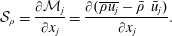 $$\begin{eqnarray}{\mathcal{S}}_{\unicode[STIX]{x1D70C}}={\displaystyle \frac{\unicode[STIX]{x2202}{\mathcal{M}}_{j}}{\unicode[STIX]{x2202}x_{j}}}={\displaystyle \frac{\unicode[STIX]{x2202}(\overline{\unicode[STIX]{x1D70C}u_{j}}-\bar{\unicode[STIX]{x1D70C}}~\bar{u}_{j})}{\unicode[STIX]{x2202}x_{j}}}.\end{eqnarray}$$
Similarly, the filtered energy equation is also a composite equation, where the variable
 $\unicode[STIX]{x1D70F}_{kk}^{\mathit{R}}/2$
is convected along with
 $\bar{E}_{\mathit{int}}$
and
 $\bar{\unicode[STIX]{x1D70C}}\bar{u}_{k}\bar{u}_{k}/2$
. A part of the SGS term
 $\unicode[STIX]{x2202}_{j}({\mathcal{K}}_{j}^{\mathit{R}}+{\mathcal{H}}_{j}^{\mathit{R}})$
in the filtered energy equation therefore corresponds to the convective transport of SGS kinetic energy
 $\unicode[STIX]{x1D70F}_{kk}^{\mathit{R}}/2$
. Similarly to the filtered momentum equation, the filtered energy equation can be reduced as well. The transport equations for filtered kinetic energy, filtered momentum and filtered velocity are used to obtain the transport equation for
 $\unicode[STIX]{x1D70F}_{kk}^{\mathit{R}}/2=(\overline{\unicode[STIX]{x1D70C}u_{k}u_{k}}-\bar{\unicode[STIX]{x1D70C}}\bar{u}_{k}\bar{u}_{k})/2$
,
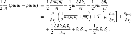 $$\begin{eqnarray}\displaystyle \frac{1}{2}{\displaystyle \frac{\unicode[STIX]{x2202}}{\unicode[STIX]{x2202}t}}\left(\overline{\unicode[STIX]{x1D70C}u_{k}u_{k}}-\bar{\unicode[STIX]{x1D70C}}\bar{u}_{k}\bar{u}_{k}\right) & = & \displaystyle \frac{1}{2}{\displaystyle \frac{\unicode[STIX]{x2202}\overline{\unicode[STIX]{x1D70C}u_{k}u_{k}}}{\unicode[STIX]{x2202}t}}-\frac{1}{2}\bar{u}_{k}{\displaystyle \frac{\unicode[STIX]{x2202}\bar{\unicode[STIX]{x1D70C}}\bar{u}_{k}}{\unicode[STIX]{x2202}t}}-\frac{1}{2}\bar{\unicode[STIX]{x1D70C}}\bar{u}_{k}{\displaystyle \frac{\unicode[STIX]{x2202}\bar{u}_{k}}{\unicode[STIX]{x2202}t}}\nonumber\\ \displaystyle & = & \displaystyle -{\displaystyle \frac{\unicode[STIX]{x2202}}{\unicode[STIX]{x2202}x_{j}}}\left(\frac{1}{2}\overline{\unicode[STIX]{x1D70C}u_{k}u_{k}u_{j}}+\overline{pu_{j}}\right)+{\mathcal{T}}\left[p,{\displaystyle \frac{\unicode[STIX]{x2202}u_{j}}{\unicode[STIX]{x2202}x_{j}}}\right]+{\displaystyle \frac{\unicode[STIX]{x2202}\bar{p}\bar{u}_{j}}{\unicode[STIX]{x2202}x_{j}}}\nonumber\\ \displaystyle & & \displaystyle +\,\frac{1}{2}{\displaystyle \frac{\unicode[STIX]{x2202}\bar{\unicode[STIX]{x1D70C}}\bar{u}_{k}\bar{u}_{k}\bar{u}_{j}}{\unicode[STIX]{x2202}x_{j}}}+\bar{u}_{k}{\mathcal{S}}_{\unicode[STIX]{x1D70C}u_{k}}-\frac{1}{2}\bar{u}_{k}\bar{u}_{k}{\mathcal{S}}_{\unicode[STIX]{x1D70C}}.\end{eqnarray}$$
By substituting
 $\unicode[STIX]{x2202}_{t}\unicode[STIX]{x1D70F}_{kk}^{\mathit{R}}/2$
in the filtered total energy equation, we obtain
 $$\begin{eqnarray}\displaystyle & & \displaystyle {\displaystyle \frac{\unicode[STIX]{x2202}}{\unicode[STIX]{x2202}t}}\left(\bar{E}_{\mathit{int}}+\frac{1}{2}\bar{\unicode[STIX]{x1D70C}}\bar{u}_{k}\bar{u}_{k}+\frac{1}{2}\unicode[STIX]{x1D70F}_{kk}^{\mathit{F}}\right)+{\displaystyle \frac{\unicode[STIX]{x2202}}{\unicode[STIX]{x2202}x_{j}}}\left(\overline{E_{\mathit{int}}u_{j}}+\overline{\unicode[STIX]{x1D70C}u_{k}u_{k}u_{j}}+\overline{pu_{j}}\right)\nonumber\\ \displaystyle & & \displaystyle \quad ={\displaystyle \frac{\unicode[STIX]{x2202}}{\unicode[STIX]{x2202}t}}\left(\bar{E}_{\mathit{int}}+\frac{1}{2}\bar{\unicode[STIX]{x1D70C}}\bar{u}_{k}\bar{u}_{k}\right)+{\displaystyle \frac{\unicode[STIX]{x2202}}{\unicode[STIX]{x2202}x_{j}}}\left(\bar{E}_{\mathit{int}}\bar{u}_{j}+\frac{1}{2}\bar{\unicode[STIX]{x1D70C}}\bar{u}_{k}\bar{u}_{k}\bar{u}_{j}+\bar{p}\bar{u}_{j}\right)+{\mathcal{S}}_{E},\end{eqnarray}$$
where the SGS terms in the transport of the quantity
 $\bar{E}_{\mathit{int}}+\bar{u}_{k}\bar{u}_{k}/2$
are
 $$\begin{eqnarray}{\mathcal{S}}_{E}={\displaystyle \frac{\unicode[STIX]{x2202}}{\unicode[STIX]{x2202}x_{j}}}\left({\mathcal{T}}[E_{\mathit{int}},u_{j}]\right)+{\mathcal{T}}\left[p,{\displaystyle \frac{\unicode[STIX]{x2202}u_{j}}{\unicode[STIX]{x2202}x_{j}}}\right]+\bar{u}_{k}{\mathcal{S}}_{\unicode[STIX]{x1D70C}u_{k}}-\frac{1}{2}\bar{u}_{k}\bar{u}_{k}{\mathcal{S}}_{\unicode[STIX]{x1D70C}}.\end{eqnarray}$$
Thus, the Reynolds-filtered LES equations can then be written as
 $$\begin{eqnarray}\frac{\unicode[STIX]{x2202}}{\unicode[STIX]{x2202}t}\left(\begin{array}{@{}c@{}}\bar{\unicode[STIX]{x1D70C}}\\ \bar{\unicode[STIX]{x1D70C}}\bar{u}_{i}\\ \bar{E}_{\mathit{int}}+\frac{1}{2}\bar{\unicode[STIX]{x1D70C}}\bar{u}_{k}\bar{u}_{k}\end{array}\right)+\frac{\unicode[STIX]{x2202}}{\unicode[STIX]{x2202}x_{j}}\left(\begin{array}{@{}c@{}}\bar{\unicode[STIX]{x1D70C}}\bar{u}_{j}\\ \bar{\unicode[STIX]{x1D70C}}\bar{u}_{i}\bar{u}_{j}+\bar{p}\unicode[STIX]{x1D6FF}_{ij}\\ \frac{1}{2}\bar{\unicode[STIX]{x1D70C}}\bar{u}_{k}\bar{u}_{k}\bar{u}_{j}+\bar{E}_{\mathit{int}}\bar{u}_{j}+\bar{p}\bar{u}_{j}\end{array}\right)+\left(\begin{array}{@{}c@{}}{\mathcal{S}}_{\unicode[STIX]{x1D70C}}\\ {\mathcal{S}}_{\unicode[STIX]{x1D70C}u_{i}}\\ {\mathcal{S}}_{E}\end{array}\right)=\left(\begin{array}{@{}c@{}}0\\ \bar{\unicode[STIX]{x1D70E}}_{\unicode[STIX]{x1D70C}u_{i}}\\ \bar{\unicode[STIX]{x1D70E}}_{E}\\ \end{array}\right),\end{eqnarray}$$
where the SGS contribution to the governing equations is
 $$\begin{eqnarray}\displaystyle & \displaystyle {\mathcal{S}}_{\unicode[STIX]{x1D70C}}={\displaystyle \frac{\unicode[STIX]{x2202}{\mathcal{T}}[\unicode[STIX]{x1D70C},u_{j}]}{\unicode[STIX]{x2202}x_{j}}}, & \displaystyle\end{eqnarray}$$
 $$\begin{eqnarray}\displaystyle & \displaystyle {\mathcal{S}}_{\unicode[STIX]{x1D70C}u_{i}}=\bar{u}_{i}{\mathcal{S}}_{\unicode[STIX]{x1D70C}}+\bar{\unicode[STIX]{x1D70C}}{\displaystyle \frac{\unicode[STIX]{x2202}{\mathcal{T}}[u_{i},u_{j}]}{\unicode[STIX]{x2202}x_{j}}}-{\mathcal{T}}\left[\unicode[STIX]{x1D70C},\frac{1}{\unicode[STIX]{x1D70C}}\frac{\unicode[STIX]{x2202}p}{\unicode[STIX]{x2202}x_{i}}\right]-\bar{\unicode[STIX]{x1D70C}}~{\mathcal{T}}[\unicode[STIX]{x1D735}\boldsymbol{\cdot }u,u_{i}], & \displaystyle\end{eqnarray}$$
 $$\begin{eqnarray}\displaystyle & \displaystyle {\mathcal{S}}_{E}=\bar{u}_{i}{\mathcal{S}}_{\unicode[STIX]{x1D70C}u_{i}}-\frac{1}{2}\bar{u}_{i}\bar{u}_{i}{\mathcal{S}}_{\unicode[STIX]{x1D70C}}+{\displaystyle \frac{\unicode[STIX]{x2202}{\mathcal{T}}[E_{\mathit{int}},u_{j}]}{\unicode[STIX]{x2202}x_{j}}}+{\mathcal{T}}[\unicode[STIX]{x1D735}\boldsymbol{\cdot }u,p]. & \displaystyle\end{eqnarray}$$
The conservation-law form of the closed convective terms is maintained and the non-conservative SGS source terms arise as a consequence of choosing to solve for the filtered velocity instead of the filtered momentum. The unclosed SGS terms are
(i) SGS mass flux,
 ${\mathcal{T}}[\unicode[STIX]{x1D70C},u_{i}]=\overline{\unicode[STIX]{x1D70C}u_{i}}-\bar{\unicode[STIX]{x1D70C}}\bar{u}_{i}$
,
(ii) SGS specific stress,
${\mathcal{T}}[u_{i},u_{j}]=\overline{u_{i}u_{j}}-\bar{u}_{i}\bar{u}_{j}$
,(iii) SGS dilatational flux,
${\mathcal{T}}[\unicode[STIX]{x1D735}\boldsymbol{\cdot }u,u_{i}]=\overline{(\unicode[STIX]{x1D735}\boldsymbol{\cdot }u)u_{i}}-(\unicode[STIX]{x1D735}\boldsymbol{\cdot }\bar{u})\bar{u}_{i}$
,(iv) SGS pressure work,
${\mathcal{T}}[\unicode[STIX]{x1D735}\boldsymbol{\cdot }u,p]=\overline{(\unicode[STIX]{x1D735}\boldsymbol{\cdot }u)p}-(\unicode[STIX]{x1D735}\boldsymbol{\cdot }\bar{u})\bar{p}$
,(v) SGS pressure–acceleration,
${\mathcal{T}}[\unicode[STIX]{x1D70C},\unicode[STIX]{x1D735}_{i}p/\unicode[STIX]{x1D70C}]/\bar{\unicode[STIX]{x1D70C}}=-(\overline{\unicode[STIX]{x1D735}_{i}p/\unicode[STIX]{x1D70C}}-\unicode[STIX]{x1D735}_{i}\bar{p}/\bar{\unicode[STIX]{x1D70C}})$
,(vi) SGS internal energy flux,
${\mathcal{T}}[E_{\mathit{int}},u_{i}]=\overline{E_{\mathit{int}}u_{i}}-\bar{E}_{\mathit{int}}\bar{u}_{i}$
.






All of the SGS terms satisfy the principle of Galilean invariance. The new SGS terms corresponding to variable-density effects not previously analysed in the LES literature are the SGS pressure–acceleration and the SGS dilatational flux. The SGS pressure–acceleration arises due to the nonlinear interaction between the pressure gradient and the density. The SGS dilatational flux arises from the nonlinear product of dilatation and velocity. We observe its similarity to the SGS pressure work, commonly referred to as the SGS pressure dilatation. The SGS pressure work has been studied extensively in the literature, because it appears in the transport equation of SGS kinetic energy, irrespective of the choice of the resolved-scale velocity variable. It should also be noted that in a multicomponent reacting flow,
 $\bar{p}$
cannot be obtained directly from
 $\bar{E}_{\mathit{int}}$
. In flows that involve non-constant
 $\unicode[STIX]{x2202}p/\unicode[STIX]{x2202}E_{int}|_{\unicode[STIX]{x1D70C}}$
, such as in the case of real/dense gas effects or multicomponent mixtures of gases with different heat capacity ratios, the term
 $\bar{p}-p(\bar{E}_{\mathit{int}},\bar{\unicode[STIX]{x1D70C}})$
requires closure as well. In such a case, the nonlinear relation between pressure and total internal energy affects the momentum equation through the filtered pressure. In this paper, we consider a single gas that obeys the ideal gas law. Therefore, the SGS term
 $\bar{p}-p(\bar{E}_{\mathit{int}},\bar{\unicode[STIX]{x1D70C}})$
does not appear in the resolved-scale momentum equation.
The primary advantage of the new equations over the conventional Reynolds-filtered formulation is the presence of a framework in which SGS contributions arising from spatial and Lagrangian density variations may be explicitly quantified. The simplified nature of the SGS terms avoids the trivariate central moment
 ${\mathcal{T}}[\unicode[STIX]{x1D70C},u_{i},u_{j}]$
in the filtered momentum equation and the quadrivariate central moment
 ${\mathcal{T}}[\unicode[STIX]{x1D70C},u_{k},u_{k},u_{j}]$
in the energy equation. This is a result of decoupling the transport equation for the SGS mass flux
 ${\mathcal{M}}_{i}$
and the SGS kinetic energy
 $\unicode[STIX]{x1D70F}_{kk}^{\mathit{R}}/2$
from the filtered momentum and the filtered energy equations. The decoupling concept for the energy equation is not restricted to a Reynolds-filtered formulation. For Favre-filtered equations, solving for the variable
 $\bar{E}_{\mathit{int}}+\bar{\unicode[STIX]{x1D70C}}\tilde{u} _{k}\tilde{u} _{k}/2$
(referred to as computable energy by Vreman Reference Vreman1995) instead of the filtered total energy
 $\bar{E}_{\mathit{int}}+\bar{\unicode[STIX]{x1D70C}}\widetilde{u_{k}u_{k}}/2$
removes
 ${\mathcal{K}}_{j}^{\mathit{F}}$
. Following a procedure similar to (2.20), we may obtain the following Favre-filtered kinetic-energy equation in which no quadrivariate central moments appear:
 $$\begin{eqnarray}{\displaystyle \frac{\unicode[STIX]{x2202}}{\unicode[STIX]{x2202}t}}\left(\frac{\bar{\unicode[STIX]{x1D70C}}\tilde{u} _{k}\tilde{u} _{k}}{2}+\bar{E}_{\mathit{int}}\right)+{\displaystyle \frac{\unicode[STIX]{x2202}}{\unicode[STIX]{x2202}x_{j}}}\left(\overline{E_{\mathit{int}}u_{j}}+\frac{\bar{\unicode[STIX]{x1D70C}}\tilde{u} _{k}\tilde{u} _{k}\tilde{u} _{j}}{2}+\bar{p}\tilde{u} _{j}\right)+\tilde{u} _{i}{\displaystyle \frac{\unicode[STIX]{x2202}\unicode[STIX]{x1D70F}_{ij}^{\mathit{F}}}{\unicode[STIX]{x2202}x_{j}}}+\left(\overline{p{\displaystyle \frac{\unicode[STIX]{x2202}u_{j}}{\unicode[STIX]{x2202}x_{j}}}}-\bar{p}{\displaystyle \frac{\unicode[STIX]{x2202}\tilde{u} _{j}}{\unicode[STIX]{x2202}x_{j}}}\right)=\bar{\unicode[STIX]{x1D70E}}_{E}.\end{eqnarray}$$
2.3 Filtered vorticity equation
The resolved-scale vorticity computed from the equations is a consequence of the choice of the resolved-scale velocity. While the Reynolds-filtered formulation computes the filtered vorticity
 $\bar{\unicode[STIX]{x1D714}}_{i}$
, in the case of the Favre-filtered velocity, the resolved-scale vorticity variable is
 $\unicode[STIX]{x1D714}_{i}^{\mathit{F}}=\unicode[STIX]{x1D735}\times \overline{\unicode[STIX]{x1D70C}u_{i}}/\bar{\unicode[STIX]{x1D70C}}$
. This is different from the filtered vorticity
 $\bar{\unicode[STIX]{x1D714}}_{i}$
, or even the Favre-filtered vorticity
 $\tilde{\unicode[STIX]{x1D714}}_{i}$
. We consider the filtered inviscid vorticity equation with the SGS terms represented as central moments,
 $$\begin{eqnarray}\displaystyle & & \displaystyle {\displaystyle \frac{\unicode[STIX]{x2202}\bar{\unicode[STIX]{x1D714}}_{i}}{\unicode[STIX]{x2202}t}}+{\displaystyle \frac{\unicode[STIX]{x2202}\bar{\unicode[STIX]{x1D714}}_{i}\bar{u}_{j}}{\unicode[STIX]{x2202}x_{j}}}+{\displaystyle \frac{\unicode[STIX]{x2202}{\mathcal{T}}[\unicode[STIX]{x1D714}_{i},u_{j}]}{\unicode[STIX]{x2202}x_{j}}}\nonumber\\ \displaystyle & & \displaystyle \quad =\bar{\unicode[STIX]{x1D714}}_{j}{\displaystyle \frac{\unicode[STIX]{x2202}\bar{u}_{i}}{\unicode[STIX]{x2202}x_{j}}}+{\mathcal{T}}\left[\unicode[STIX]{x1D714}_{j},{\displaystyle \frac{\unicode[STIX]{x2202}u_{i}}{\unicode[STIX]{x2202}x_{j}}}\right]-\unicode[STIX]{x1D716}_{ijk}\left({\displaystyle \frac{\unicode[STIX]{x2202}(\overline{1/\unicode[STIX]{x1D70C}})}{\unicode[STIX]{x2202}x_{j}}}{\displaystyle \frac{\unicode[STIX]{x2202}\bar{p}}{\unicode[STIX]{x2202}x_{k}}}+{\mathcal{T}}\left[{\displaystyle \frac{\unicode[STIX]{x2202}(1/\unicode[STIX]{x1D70C})}{\unicode[STIX]{x2202}x_{j}}},{\displaystyle \frac{\unicode[STIX]{x2202}p}{\unicode[STIX]{x2202}x_{k}}}\right]\right).\end{eqnarray}$$
The SGS contributions to vorticity flux, vortex stretching and baroclinic torque can be seen to appear separately. We observe that the curl of the SGS pressure–acceleration is the SGS baroclinic torque,
 $$\begin{eqnarray}\displaystyle -\unicode[STIX]{x1D716}_{ijk}{\mathcal{T}}\left[{\displaystyle \frac{\unicode[STIX]{x2202}}{\unicode[STIX]{x2202}x_{j}}}\left(\frac{1}{\unicode[STIX]{x1D70C}}\right),{\displaystyle \frac{\unicode[STIX]{x2202}p}{\unicode[STIX]{x2202}x_{k}}}\right]=\unicode[STIX]{x1D716}_{ijk}{\displaystyle \frac{\unicode[STIX]{x2202}}{\unicode[STIX]{x2202}x_{j}}}\left(\frac{1}{\bar{\unicode[STIX]{x1D70C}}}{\mathcal{T}}\left[\unicode[STIX]{x1D70C},\frac{1}{\unicode[STIX]{x1D70C}}{\displaystyle \frac{\unicode[STIX]{x2202}p}{\unicode[STIX]{x2202}x_{k}}}\right]\right). & & \displaystyle\end{eqnarray}$$
The SGS acceleration field contributes to the filtered vorticity and more generally to the entire filtered velocity-gradient tensor. The symmetric part of the SGS pressure–acceleration-gradient tensor
 $\unicode[STIX]{x2202}_{j}({\mathcal{T}}[\unicode[STIX]{x1D70C},\unicode[STIX]{x2202}_{k}p/\unicode[STIX]{x1D70C}]/\bar{\unicode[STIX]{x1D70C}})$
appears as a source term in the filtered strain-rate
 $\bar{\unicode[STIX]{x1D61A}}_{ij}$
equation. The SGS pressure–acceleration, due its dependence on both the pressure and the density field, can distinguish between entropic and acoustic density fluctuations. This can be important for modelling (Rubinstein & Erlebacher Reference Rubinstein and Erlebacher1997; Hamba Reference Hamba1999).
Therefore, we see that the curls of the Reynolds-filtered and Favre-filtered velocities represent physically different resolved-scale vorticity variables. In particular, the SGS baroclinic torque affects the Reynolds-filtered vorticity
 $\bar{\unicode[STIX]{x1D714}}_{i}$
but does not explicitly affect
 $\unicode[STIX]{x1D714}_{i}^{\mathit{F}}$
.
2.4 Filtered scalar advection equation
It is important to discuss the scalar advection equation in the context of variable-density flows. For example, flows that involve multicomponent mixing and combustion require advection of species densities. When a combustion model is used, a reaction progress variable is advected. The filtered inviscid scalar advection equations with
 $\tilde{u} _{i}$
and
 $\bar{u}_{i}$
are
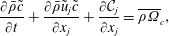 $$\begin{eqnarray}\displaystyle & \displaystyle {\displaystyle \frac{\unicode[STIX]{x2202}\bar{\unicode[STIX]{x1D70C}}\tilde{c}}{\unicode[STIX]{x2202}t}}+{\displaystyle \frac{\unicode[STIX]{x2202}\bar{\unicode[STIX]{x1D70C}}\tilde{u} _{j}\tilde{c}}{\unicode[STIX]{x2202}x_{j}}}+{\displaystyle \frac{\unicode[STIX]{x2202}{\mathcal{C}}_{j}}{\unicode[STIX]{x2202}x_{j}}}=\overline{\unicode[STIX]{x1D70C}\unicode[STIX]{x1D6FA}}_{c}, & \displaystyle\end{eqnarray}$$
 $$\begin{eqnarray}\displaystyle & \displaystyle {\displaystyle \frac{\unicode[STIX]{x2202}\bar{\unicode[STIX]{x1D70C}}\tilde{c}}{\unicode[STIX]{x2202}t}}+{\displaystyle \frac{\unicode[STIX]{x2202}\bar{\unicode[STIX]{x1D70C}}\bar{u}_{j}\tilde{c}}{\unicode[STIX]{x2202}x_{j}}}+{\displaystyle \frac{\unicode[STIX]{x2202}{\mathcal{T}}[\unicode[STIX]{x1D70C}c,u_{j}]}{\unicode[STIX]{x2202}x_{j}}}=\overline{\unicode[STIX]{x1D70C}\unicode[STIX]{x1D6FA}}_{c}, & \displaystyle\end{eqnarray}$$
where the scalar
 $c$
is the advected variable. Here,
 $\unicode[STIX]{x1D6FA}_{c}$
represents the source term in the transport equation of the scalar
 $c$
. The unclosed term in the Favre-filtered velocity scalar equation can be expressed with central moments similarly to the SGS stress
 $\unicode[STIX]{x1D70F}_{ij}^{\mathit{F}}$
,
 $$\begin{eqnarray}\displaystyle {\mathcal{C}}_{j} & = & \displaystyle \overline{\unicode[STIX]{x1D70C}u_{j}c}-\bar{\unicode[STIX]{x1D70C}}\tilde{u} _{j}\tilde{c}=\bar{\unicode[STIX]{x1D70C}}(\widetilde{cu_{j}}-\tilde{c}\tilde{u} _{j})\end{eqnarray}$$
 $$\begin{eqnarray}\displaystyle & = & \displaystyle \bar{\unicode[STIX]{x1D70C}}{\mathcal{T}}[c,u_{j}]+{\mathcal{T}}[\unicode[STIX]{x1D70C},u_{j},c]-{\displaystyle \frac{1}{\bar{\unicode[STIX]{x1D70C}}}}{\mathcal{T}}[\unicode[STIX]{x1D70C},u_{j}]{\mathcal{T}}[\unicode[STIX]{x1D70C},c].\end{eqnarray}$$
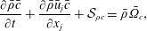
In the equations above, the Favre-filtered scalar is transported. It is also possible to derive the transport equation for the filtered scalar and express the equation in a conservation-law form,
 $$\begin{eqnarray}{\displaystyle \frac{\unicode[STIX]{x2202}\bar{\unicode[STIX]{x1D70C}}\bar{c}}{\unicode[STIX]{x2202}t}}+{\displaystyle \frac{\unicode[STIX]{x2202}\bar{\unicode[STIX]{x1D70C}}\bar{u}_{j}\bar{c}}{\unicode[STIX]{x2202}x_{j}}}+{\mathcal{S}}_{\unicode[STIX]{x1D70C}c}=\bar{\unicode[STIX]{x1D70C}}\bar{\unicode[STIX]{x1D6FA}}_{c},\end{eqnarray}$$
where the SGS contribution
 ${\mathcal{S}}_{\unicode[STIX]{x1D70C}c}$
is expressed in the form of central moments as
 $$\begin{eqnarray}{\mathcal{S}}_{\unicode[STIX]{x1D70C}c}=\bar{\unicode[STIX]{x1D70C}}{\displaystyle \frac{\unicode[STIX]{x2202}{\mathcal{T}}[c,u_{j}]}{\unicode[STIX]{x2202}x_{j}}}+\bar{c}~{\mathcal{S}}_{\unicode[STIX]{x1D70C}}-\bar{\unicode[STIX]{x1D70C}}{\mathcal{T}}\left[c,{\displaystyle \frac{\unicode[STIX]{x2202}u_{j}}{\unicode[STIX]{x2202}x_{j}}}\right].\end{eqnarray}$$
Equation (2.34) is obtained by decoupling the inviscid transport equation for
 ${\mathcal{T}}[\unicode[STIX]{x1D70C},c]$
from (2.30), similarly to the procedure we adopt for the resolved-scale momentum and the energy equations. We observe that the use of filtered velocity does not involve the trivariate moment
 ${\mathcal{T}}[\unicode[STIX]{x1D70C},u_{j},c]$
in the unclosed terms. In the case of the Favre-filtered scalar and the filtered velocity, the effect of density appears in the SGS conserved scalar flux
 ${\mathcal{T}}[\unicode[STIX]{x1D70C}c,u_{j}]$
. If the filtered scalar is transported, the effect of the SGS mass flux and the SGS dilatation can be represented explicitly.
3 Direct numerical simulations
We carry out direct numerical simulations (DNS) of decaying isotropic compressible turbulence to study variable-density and dilatation effects on the flow. The data from the DNS will be filtered to evaluate the relative importance of the variable-density SGS terms. Two flow cases are investigated, as listed in table 1. The first case is canonical decaying compressible turbulence, where the initial thermodynamic fluctuations are homentropic, i.e. the flow has spatially uniform entropy. The second case is compressible variable-density decaying turbulence, where the initial density field is isotropic, inhomogeneous and corresponds to a double-
 $\unicode[STIX]{x1D6FF}$
probability distribution function (p.d.f.). In the first case, density fluctuations arise primarily out of compressibility, while in the second case, density fluctuations are primarily a consequence of the mixing of fluid of varying density. A variant of the second case with stronger initial density fluctuations is also simulated. In these simulations, the double-
 $\unicode[STIX]{x1D6FF}$
p.d.f. density field initialization corresponds to thermal inhomogeneity, which is different from binary mixing between two different fluid species with associated species mass diffusion. Therefore, Schmidt-number effects are outside the scope of these simulations. Since the imprints of initial conditions in triperiodic decaying compressible flows can persist throughout the simulation time (Ristorcelli & Blaisdell Reference Ristorcelli and Blaisdell1997), the initial conditions in the current simulations are carefully designed to avoid impulsive forcing of the flow field that might corrupt the high-order statistics.
Primary flow cases simulated for SGS analysis.

3.1 Simulation set-up and numerical method
We solve the compressible Navier–Stokes equations on a triperiodic domain with initialization for the variables
 $\unicode[STIX]{x1D70C},u_{i},p$
. The ideal gas law
 $p=\unicode[STIX]{x1D70C}RT$
is used to compute the temperature field. Transport properties such as viscosity are taken to be constant, to avoid the influence of variable-density fluctuations on viscous transport processes. The viscous terms in the momentum and energy equations are
 $\unicode[STIX]{x1D70E}_{\unicode[STIX]{x1D70C}u_{i}}=-\unicode[STIX]{x1D707}(\unicode[STIX]{x2202}_{j}\unicode[STIX]{x1D61A}_{ij}-2/3~\unicode[STIX]{x2202}_{j}\unicode[STIX]{x1D61A}_{kk}\unicode[STIX]{x1D6FF}_{ij})$
and
 $\unicode[STIX]{x1D70E}_{E}=-c_{p}\unicode[STIX]{x1D707}/Pr~\unicode[STIX]{x2202}_{j}T$
respectively. Here,
 $\unicode[STIX]{x1D61A}_{ij}$
is the strain-rate tensor and
 $c_{p}$
is the specific heat capacity. We assume a calorically perfect gas with constant
 $c_{p}=1.003~\text{kJ}~\text{kg}^{-1}~\text{K}$
and a Prandtl number of 0.72,
 $$\begin{eqnarray}\frac{\unicode[STIX]{x2202}}{\unicode[STIX]{x2202}t}\left(\begin{array}{@{}c@{}}\unicode[STIX]{x1D70C}\\ \unicode[STIX]{x1D70C}u_{i}\\ \frac{1}{2}\unicode[STIX]{x1D70C}u_{k}u_{k}+E_{\mathit{int}}\end{array}\right)+\frac{\unicode[STIX]{x2202}}{\unicode[STIX]{x2202}x_{j}}\left(\begin{array}{@{}c@{}}\unicode[STIX]{x1D70C}u_{j}\\ \unicode[STIX]{x1D70C}u_{i}u_{j}+p\unicode[STIX]{x1D6FF}_{ij}\\ \frac{1}{2}\unicode[STIX]{x1D70C}u_{k}u_{k}+E_{\mathit{int}}u_{j}+pu_{j}\end{array}\right)+\left(\begin{array}{@{}c@{}}0\\ \unicode[STIX]{x1D70E}_{\unicode[STIX]{x1D70C}u_{i}}\\ \unicode[STIX]{x1D70E}_{E}\end{array}\right)=\left(\begin{array}{@{}c@{}}0\\ 0\\ 0\end{array}\right).\end{eqnarray}$$
A triperiodic grid with 512 points in each coordinate direction is used for the simulations. Three cases are considered (table 1) with a turbulent Mach number
 $M_{t}$
of 0.3, which is chosen as representative of high-speed turbulent boundary layers (Lagha et al.
Reference Lagha, Kim, Eldredge and Zhong2011). The initial velocity field is identical for all cases and is initialized by extracting the solenoidal velocity component from a precursor simulation of compressible decaying turbulence simulation whose velocity derivative skewness has saturated to a value close to 0.5. Saturation in skewness implies that the rate of vorticity production via vortex stretching has stabilized and the flow has evolved from an artificial state into a turbulent state with realistic nonlinear dynamics. The precursor simulation therefore ensures that the flows initialized in this study are closer to a realistic turbulent flow compared with a random isotropic velocity field. The precursor simulation is initialized with a
 $k^{2}\exp (-2(k/k_{0})^{2})$
radial spectrum with
 $Re_{\unicode[STIX]{x1D706}}=100,M_{t}=0.3,k_{0}/L=6$
and simulated to
 $t/t_{eddy}=3.0$
.
The initial density, pressure and temperature fields are initialized in two different ways, denoted by IC1 and IC2. In IC1, the initial pressure field is obtained from the incompressible Poisson equation using the volume-averaged density. The density field is then initialized with
 $p/\unicode[STIX]{x1D70C}^{\unicode[STIX]{x1D6FE}}=\langle p\rangle /\langle \unicode[STIX]{x1D70C}\rangle ^{\unicode[STIX]{x1D6FE}}$
(Ristorcelli & Blaisdell Reference Ristorcelli and Blaisdell1997; Samtaney, Pullin & Kosović Reference Samtaney, Pullin and Kosović2001). It should be noted that only the solenoidal velocity field from the precursor simulation is used for initialization. This is because with IC1 thermodynamic fields, the time evolution of mean dilatation variance with zero initial dilatation is nearly identical to that from a non-zero initial dilatation obtained from small-parameter expansion about
 $M_{t}$
(Ristorcelli & Blaisdell Reference Ristorcelli and Blaisdell1997). The two curves from zero and non-zero initial dilatation are found to nearly overlap for
 $t/t_{eddy}>0.3$
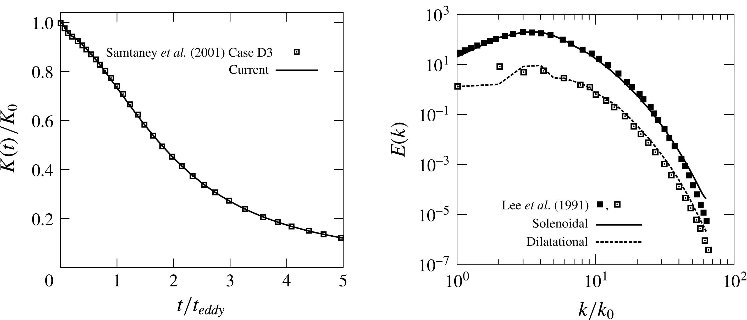
. The turbulent kinetic-energy decay in compressible turbulence using IC1 is compared with results from Samtaney et al. (Reference Samtaney, Pullin and Kosović2001) in the Appendix.
IC2 corresponds to an isotropic double-
 $\unicode[STIX]{x1D6FF}$
distribution of the density field with the volume divided into two regions of densities,
 $\unicode[STIX]{x1D70C}_{1}$
and
 $\unicode[STIX]{x1D70C}_{2}$
, with a smooth interface. Similar scalar fields have been used previously in the work of Sandoval (Reference Sandoval1995) and Livescu & Ristorcelli (Reference Livescu and Ristorcelli2007). The scalar field is generated with non-zero spectral content for
 $2\leqslant kL\leqslant 4$
, where
 $L$
is the length of the periodic domain. To generate a smooth interface, the field is filtered with an exponential filter with
 $k_{c}L=4$
, resulting in a
 $\unicode[STIX]{x1D70C}$
p.d.f. that deviates slightly from a strict double-
 $\unicode[STIX]{x1D6FF}$
distribution. Smoothing of the
 $\unicode[STIX]{x1D70C}$
interface changes the mean and variance of the density distribution from 1.0 and 0.25 to 1.017 and 0.235 respectively. The Atwood number
 $A=(\unicode[STIX]{x1D70C}_{2}+\unicode[STIX]{x1D70C}_{1})/(\unicode[STIX]{x1D70C}_{2}-\unicode[STIX]{x1D70C}_{1})$
is an important parameter in quantifying the strength of hydrodynamic instability in stratified flows; a volumetric mean density
 $\langle \unicode[STIX]{x1D70C}\rangle =1.0$
is used to calculate
 $\unicode[STIX]{x1D70C}_{1}$
and
 $\unicode[STIX]{x1D70C}_{2}$
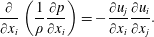
. Cases 2a and 2b use IC2, but differ in the Atwood number. Case 2b has a larger Atwood number than case 2a and, as expected, exhibits more pronounced variable-density effects. The largest value of Atwood number considered here corresponds to a density ratio of approximately 6, which is a typical of light/heavy fluid mixing in industrial applications. Larger density ratios exist in combustion and multiphase systems, and are expected to produce stronger variable-density effects. The pressure in IC2 is determined by solving the inviscid variable-density Poisson equation. This equation is obtained by ensuring that the initial conditions do not provide a source of Lagrangian change in fluid density,
 $\text{D}(\unicode[STIX]{x2202}_{j}u_{j})/\text{D}t=0$
. The pressure at time
 $t=0$
therefore satisfies
 $$\begin{eqnarray}\frac{\unicode[STIX]{x2202}}{\unicode[STIX]{x2202}x_{i}}\left(\frac{1}{\unicode[STIX]{x1D70C}}\frac{\unicode[STIX]{x2202}p}{\unicode[STIX]{x2202}x_{i}}\right)=-\frac{\unicode[STIX]{x2202}u_{j}}{\unicode[STIX]{x2202}x_{i}}\frac{\unicode[STIX]{x2202}u_{i}}{\unicode[STIX]{x2202}x_{j}}.\end{eqnarray}$$
We restrict the initial
 $u_{i},\unicode[STIX]{x1D70C}$
fields to large length scales. The velocity field from the precursor simulation and the generated density field are filtered using a sharp spectral filter with
 $k_{c}L=32$
. This ensures that the small scales in the density and velocity fields develop from the initial conditions together via vortex stretching and baroclinic torque. The viscosity is specified such that the initial Taylor length scale Reynolds number
 $Re_{\unicode[STIX]{x1D706}}$
is 500. The Taylor length scale Reynolds number is large because the initial velocity spectrum is non-zero at low wavenumbers
 $kL<32$
, resulting in a large initial Taylor length scale
 $\unicode[STIX]{x1D706}$
. After the transient, the energy spectrum becomes broadband and
 $Re_{\unicode[STIX]{x1D706}}$
decreases. At
 $t/t_{eddy}=3$
, the Taylor length scale Reynolds number reduces to
 $Re_{\unicode[STIX]{x1D706}}=85$
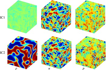
. The fields corresponding to the initial conditions are visualized in figure 1.
Direct numerical simulation initialization; the
 $\unicode[STIX]{x1D70C}$
,
 $u$
and
 $p$
fields are shown.

A finite-volume scheme is employed to solve (3.1). The convective flux is evaluated using a stable low-dissipation scheme based on the kinetic-energy consistent method developed by Subbareddy & Candler (Reference Subbareddy and Candler2009). A gradient reconstruction method described by Subbareddy, Bartkowicz & Candler (Reference Subbareddy, Bartkowicz and Candler2014) is used to make the symmetric part of the convective flux formally sixth-order accurate. In regions of strong compression (shocklets), a Ducros-type shock sensor adds dissipation to the convective flux using the non-symmetric part of the modified Steger–Warming flux-vector splitting scheme. The details of the flux scheme can be found in MacCormack (Reference MacCormack2014) and Candler, Subbareddy & Brock (Reference Candler, Subbareddy and Brock2015). The viscous fluxes are computed using a second-order central scheme and use compact stencil second-order least-squares gradients. The low-storage third-order-accurate strong stability preserving Runge–Kutta scheme (Gottlieb, Shu & Tadmor Reference Gottlieb, Shu and Tadmor2001) is used for time integration. A CFL (Courant–Friedrichs–Lewy) number of 0.7 based on the local fast characteristic wave speed is used.
3.2 Time histories and spatial statistics
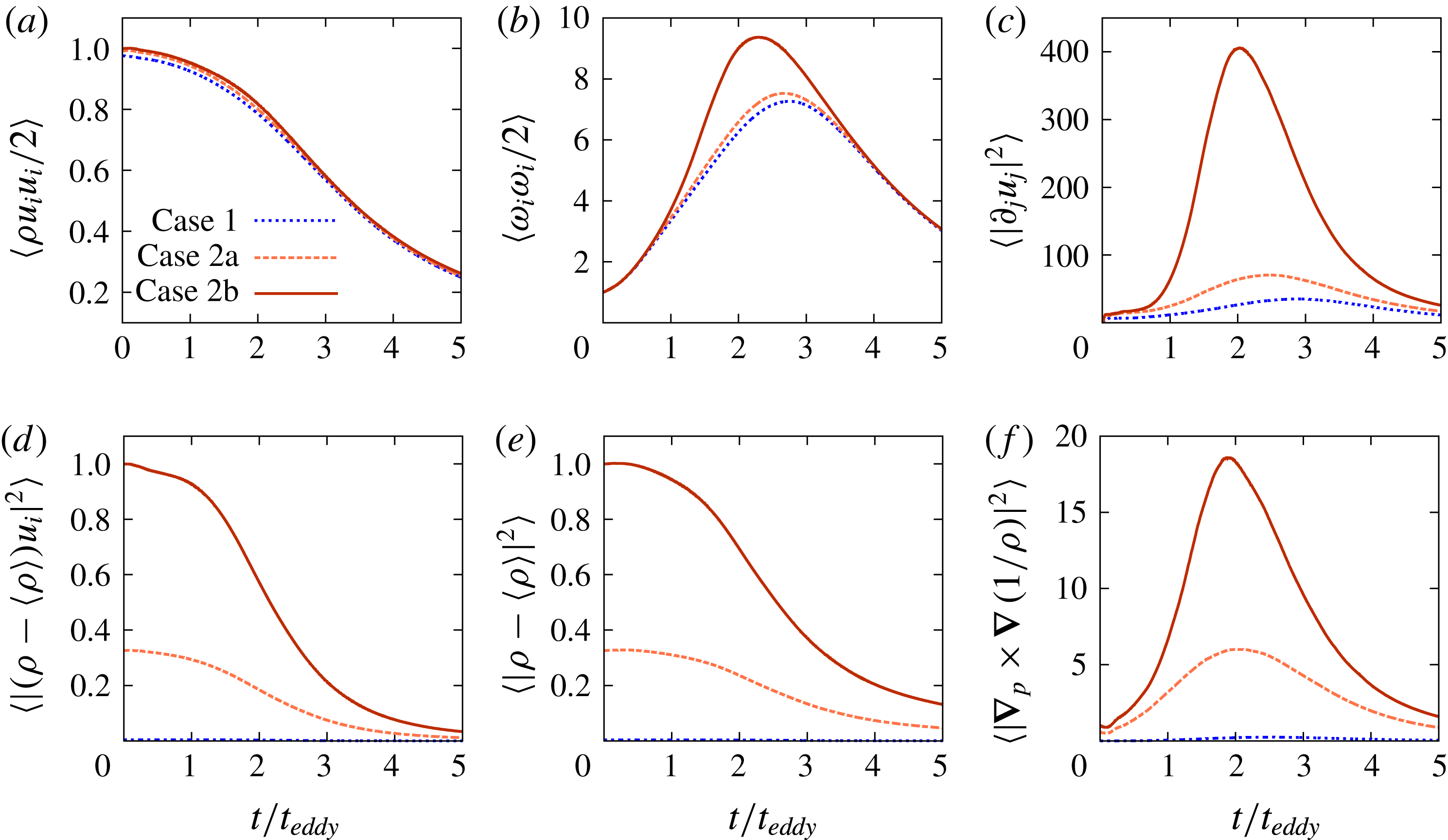
Volume-averaged statistics from the three cases simulated are shown in figure 2. The time histories of six physical quantities are plotted: (a) kinetic energy, (b) enstrophy, (c) dilatation variance, (d) mass flux variance, (e) density variance and (f) baroclinic-torque variance. The volume averages of dilatation, mass flux and baroclinic torque are numerically close to zero and, hence, variances of these quantities are plotted. All of the curves are normalized by the value corresponding to case 2b at time
 $t=0$
. While the volume-averaged kinetic-energy curves nearly overlap, quantities based on velocity gradients, namely the enstrophy and dilatation variance, exhibit prominent differences during
 $1\leqslant t/t_{eddy}\leqslant 4$
. This occurs when small velocity scales are produced by vortex stretching and variable-density mixing effects are active. Later, when mixing homogenizes the density field, the curves of kinetic energy, enstrophy and dilatation variance for cases 2a and 2b begin to converge with the case 1 curves.
Time histories of volume-averaged quantities. (a) Energy, (b) enstrophy, (c) dilatation, (d) mass flux variance, (e) density variance and (f) baroclinic-torque magnitude.
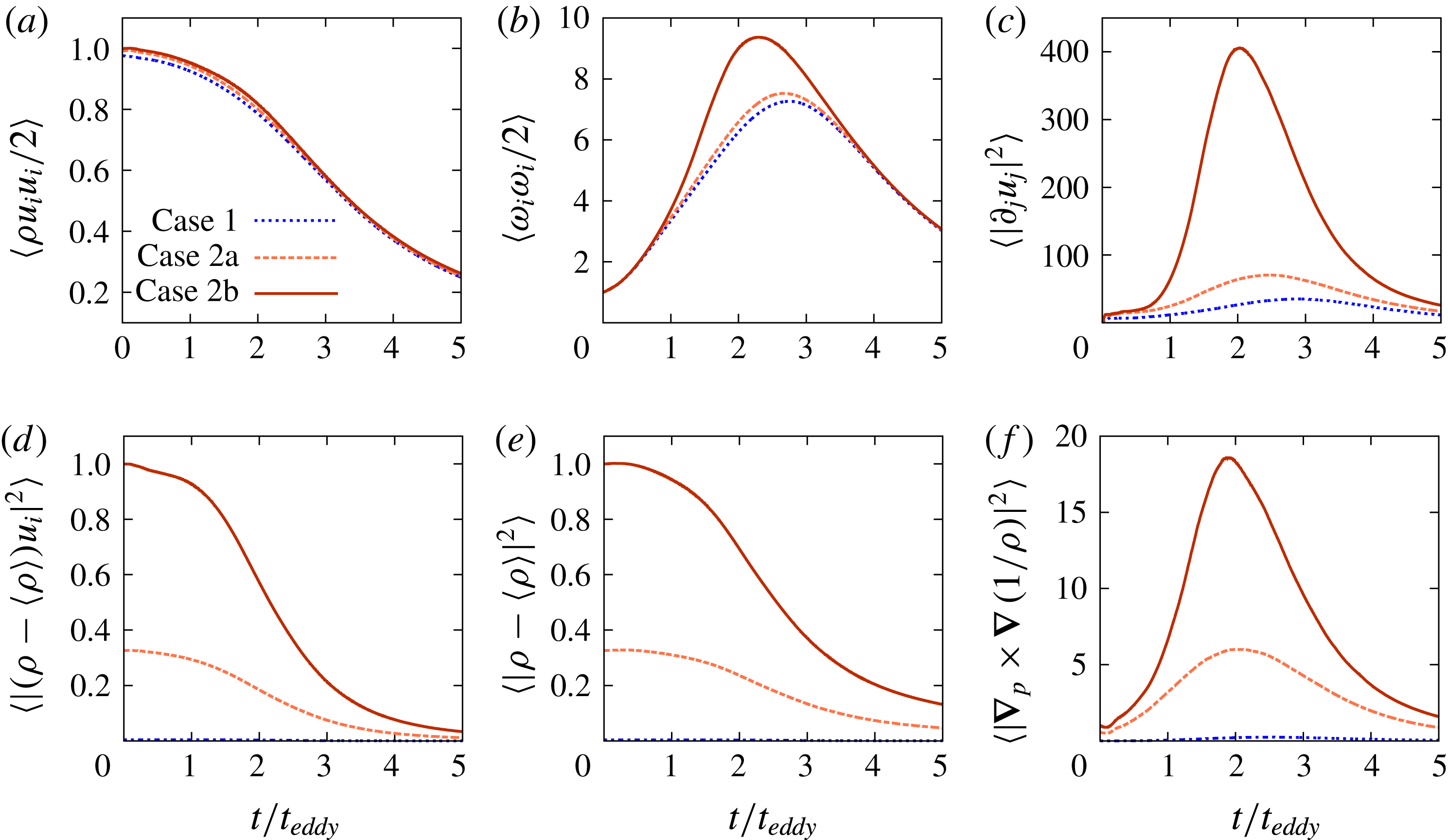
Velocity-gradient-based statistics are found to be more strongly affected by variable-density effects. In the case of enstrophy, the differences can be attributed to production of vorticity by baroclinic torque, which is the curl of the pressure-gradient acceleration. Baroclinic-torque-generated vorticity is further stretched by the background strain, thus compounding the enstrophy generation process. We also note that the differences in the curves are discernible only after one eddy turnover time, indicating the absence of impulsively generated enstrophy by the initial conditions. The increase in dilatation variance (figure 2
c) in cases 2a and 2b can be explained by the pressure-gradient acceleration. The pressure-gradient acceleration tensor
 ${\mathcal{A}}_{ij}=\unicode[STIX]{x2202}_{j}(\unicode[STIX]{x2202}_{i}p/\unicode[STIX]{x1D70C})$
appears in the velocity-gradient transport equation. The antisymmetric part,
 ${\mathcal{A}}_{ij}-{\mathcal{A}}_{ji}$
, is associated with baroclinic torque, and the corresponding term in the dilatation rate equation is the trace of the tensor
 ${\mathcal{A}}_{ii}$
. The symmetric part,
 ${\mathcal{A}}_{ij}+{\mathcal{A}}_{ji}$
, contributes to the rate of change of the strain-rate tensor. The fluctuating mass flux variance and the density fluctuation variance decay monotonically, but have transience that lasts approximately two eddy turnover times, marked by an inflection point in their respective curves. The fluctuating mass flux is also the mean fluctuating Favre-filtered velocity and represents the spatial correlation of the density and velocity fields. The initial density variance in case 1 is seen to be extremely small relative to cases 2a and 2b, and suggests that the variable-density effects in compressible decaying turbulence are expected to be small for
 $M_{t}=0.3$
.
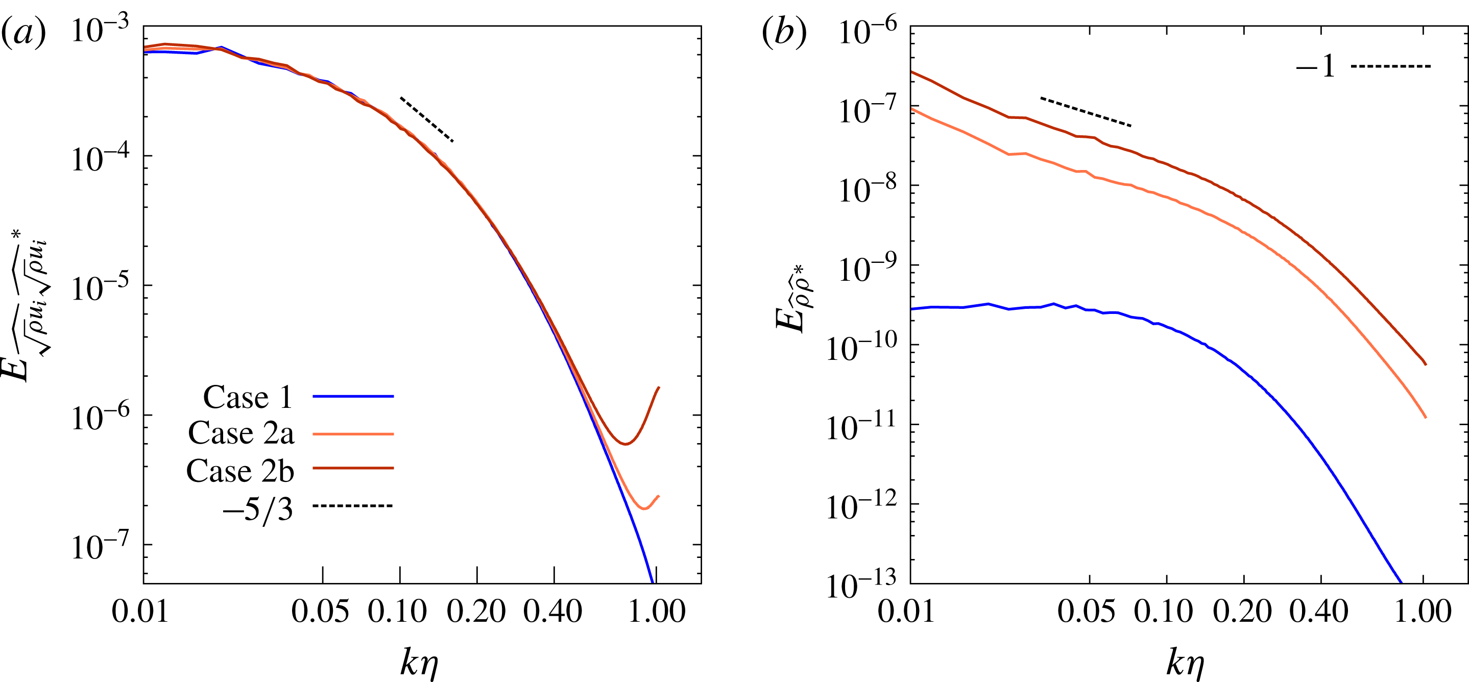
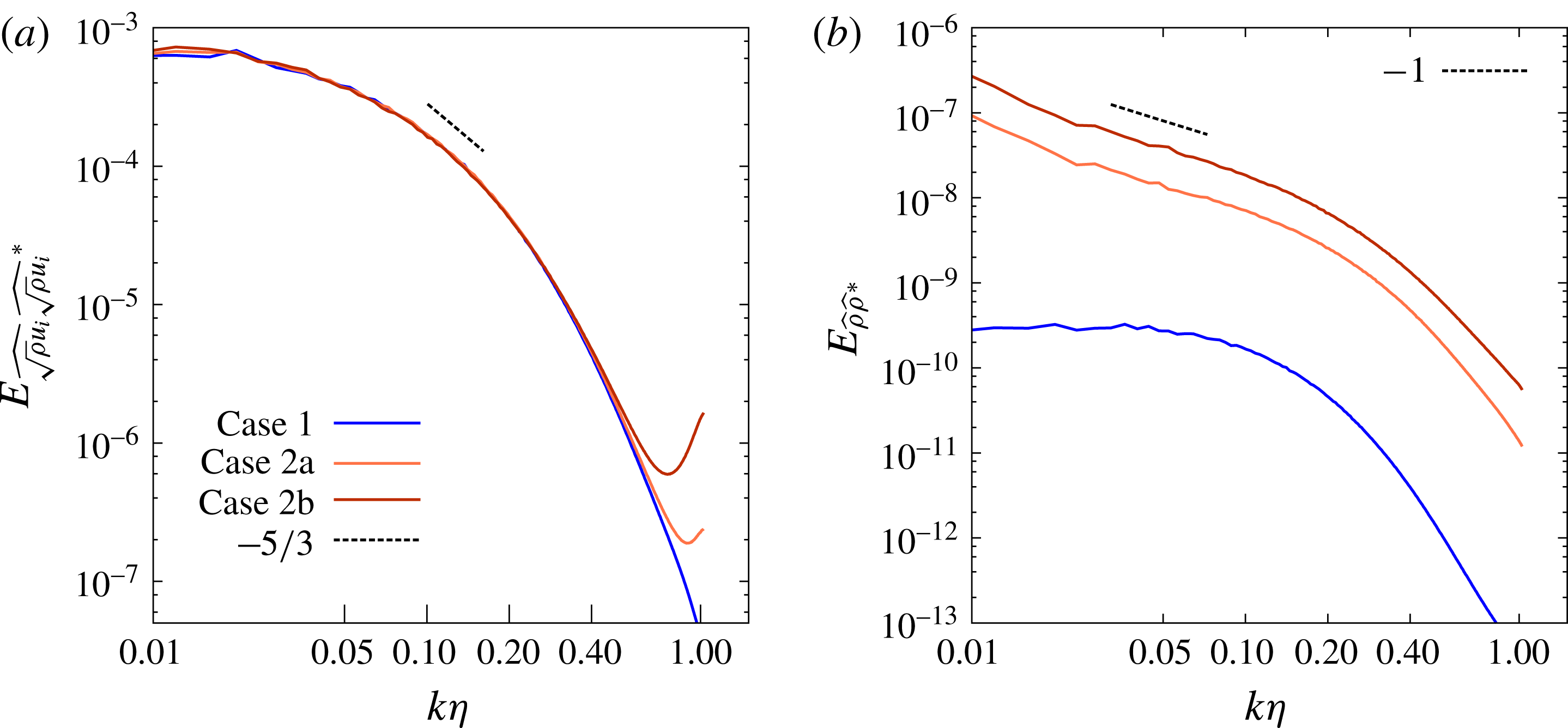
The kinetic-energy radial spectra and the energy spectral density of the density field at
 $t/t_{eddy}=3.0$
are plotted in figure 3. The flow field at this time contains a small inertial subrange with a
 $k^{-5/3}$
slope present approximately in the range
 $0.2\geqslant k\unicode[STIX]{x1D702}\geqslant 0.1$
. The presence of initial thermal-density inhomogeneity increases the content at small velocity scales, but the
 $k^{-5/3}$
spectrum is preserved. Increasing strength of density fluctuations leads to increased rate of kinetic-energy transfer to higher wavenumbers. This is also reflected in the aliasing error that develops at high wavenumbers due to the use of a low-dissipation central numerical scheme in the simulations. The density field spectrum shows that the content in the large scales for case 1 is relatively flat (
 ${\sim}k^{0}$
), while cases 2a and 2b, which involve mixing of variable-density fluids, exhibit a
 $k^{-1}$
behaviour at low wavenumbers. This may be interpreted as the Batchelor
 $k^{-1}$
viscous–convective scaling in the high-Schmidt-number limit as the effective diffusivity for density is zero (Donzis, Sreenivasan & Yeung Reference Donzis, Sreenivasan and Yeung2010).
Three-dimensional shell-averaged radial spectra of kinetic energy (a) and energy spectral density of the density (b) at
 $t/t_{eddy}=3.0$
.
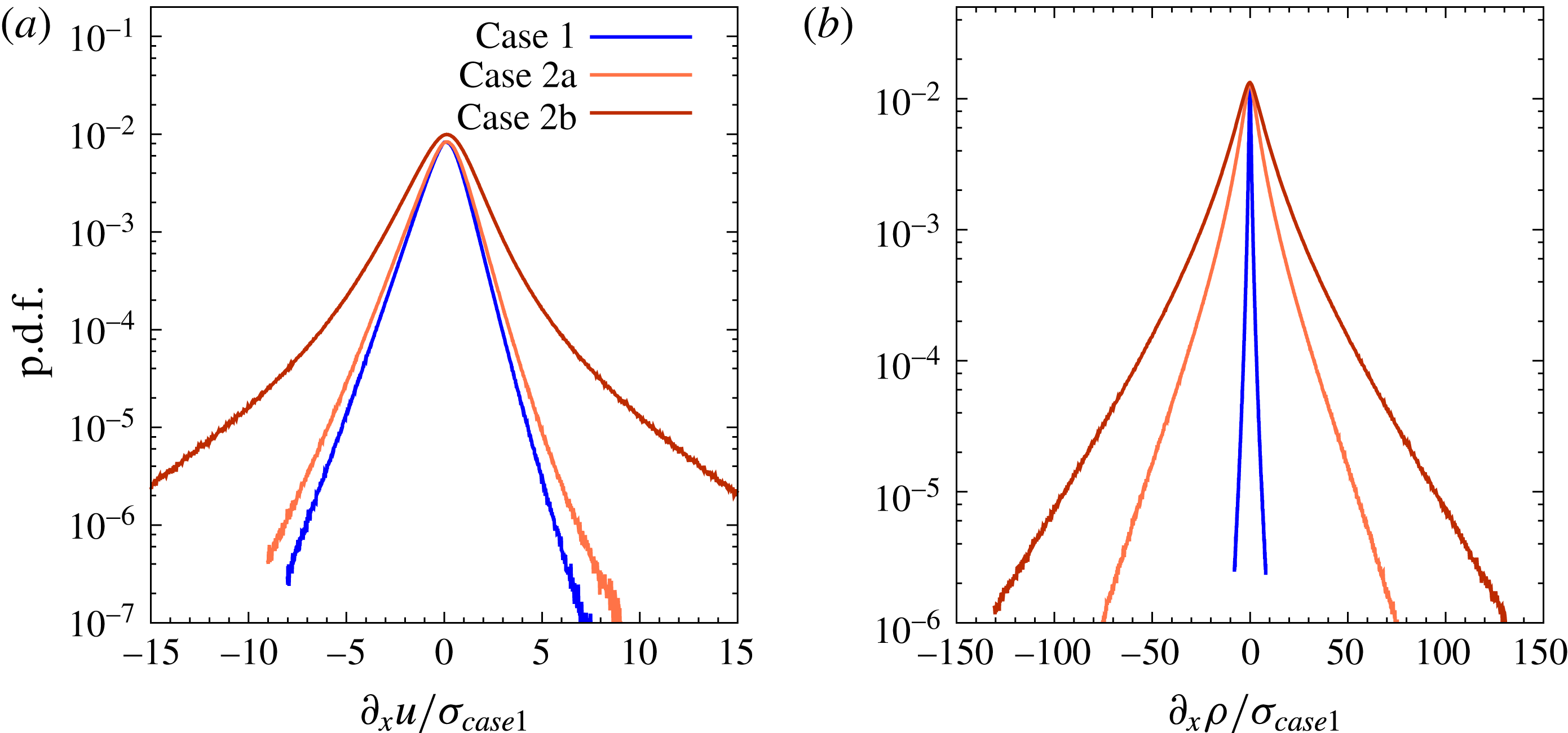
Probability distribution functions of the
 $x$
gradients of the
 $x$
components of the velocity (a) and density (b) fields.
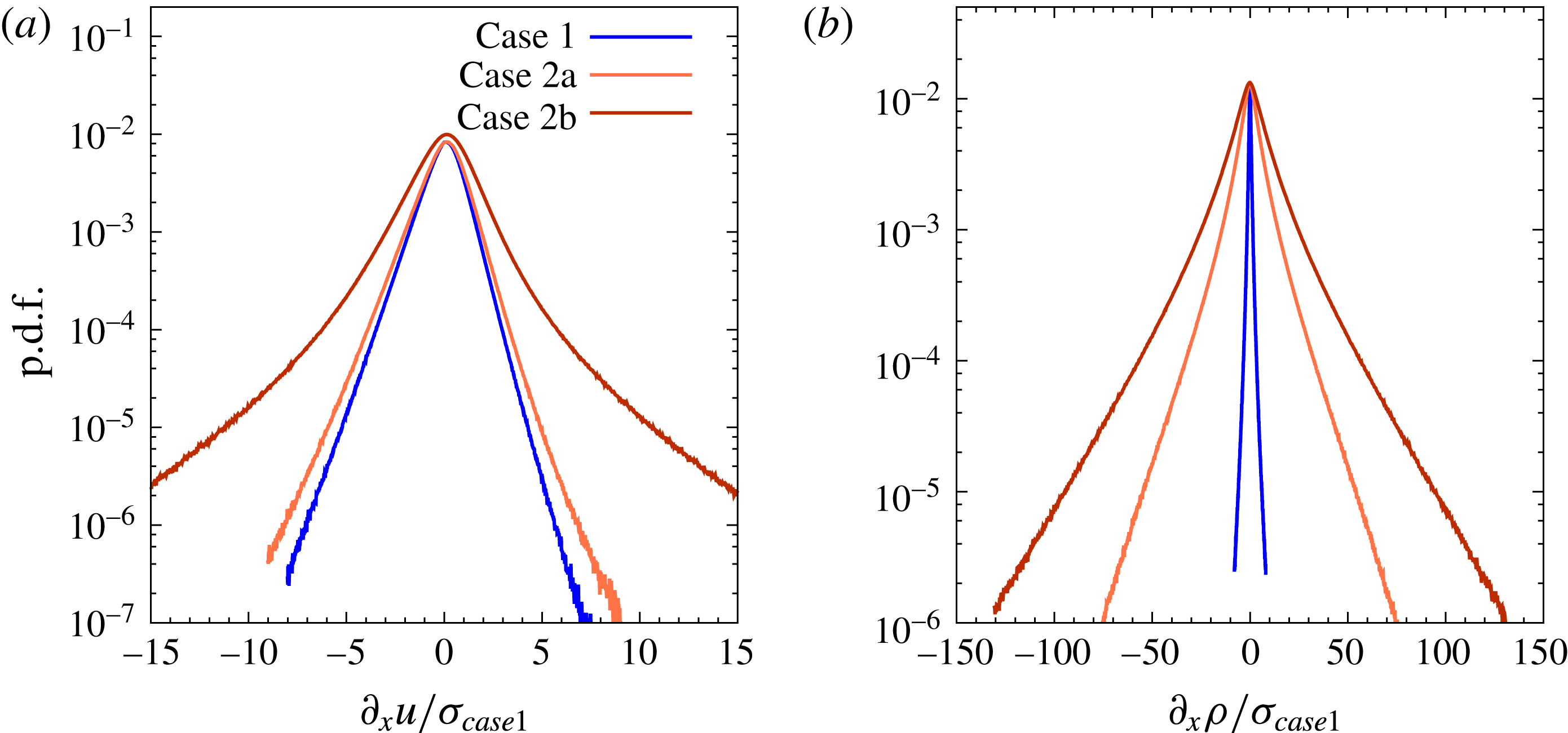
Figure 4 shows the effect of variable-density mixing on the intermittency of the flow fields. Probability distribution functions of the
 $x$
gradients of the
 $x$
components of the velocity and density are plotted. The mean values have been subtracted and the
 $x$
-axis is scaled with the standard deviation for case 1. Variable-density effects are seen to increase the probability of occurrence of tail events and have distributions with larger standard deviations. The
 $\unicode[STIX]{x2202}_{x}u$
and
 $\unicode[STIX]{x2202}_{x}\unicode[STIX]{x1D70C}$
p.d.f.s show that all cases have a high degree of super-Gaussian (leptokurtic) character, indicating the presence of intermittency representative of high-
 $Re$
turbulence (Schumacher et al.
Reference Schumacher, Scheel, Krasnov, Donzis, Yakhot and Sreenivasan2014). The values of the kurtosis of the
 $\unicode[STIX]{x2202}_{x}u$
and
 $\unicode[STIX]{x2202}_{x}\unicode[STIX]{x1D70C}$
fields in case 1 are 18.8 and 22.7 respectively. In case 2b, the values of the kurtosis for both distributions reduce to 13.0 and 16.7 respectively, due to increased probability of the occurrence of tail events. In comparison, the kurtosis of a Gaussian distribution is 3.
4 Variable-density SGS analysis
In this section, we explicitly filter the DNS flow fields to study the SGS terms that appear in the Favre-filtered and Reynolds-filtered momentum equations. The first subsection compares the two resolved-scale velocity fields in Fourier and physical space. The second subsection compares the importance of the variable-density SGS terms with respect to the constant-density SGS terms. Central moments that involve
 $\unicode[STIX]{x1D70C}$
and
 $\unicode[STIX]{x1D735}\boldsymbol{\cdot }u$
as one of the variables under the filter operator are referred to as variable-density SGS terms. Terms that involve the SGS specific stress
 ${\mathcal{T}}[u_{i},u_{j}]=\overline{u_{i}u_{j}}-\bar{u}_{i}\bar{u}_{j}$
are referred to as constant-density SGS terms. This is the first study that computes the effect of the small-scale density variations on the large-scale momentum in compressible turbulent mixing of variable-density fluids. We restrict the results to a budget analysis, and no a priori assessment of SGS closures is conducted. Similarly, as mentioned above, the effect of implicit filtering associated with an LES discretization is not discussed.
The time histories of dilatation and enstrophy suggest that the flows reach a state of decay after two eddy turnover times. Therefore, we carry out the variable-density SGS analysis of the instantaneous flow field at
 $t/t_{eddy}=3.0$
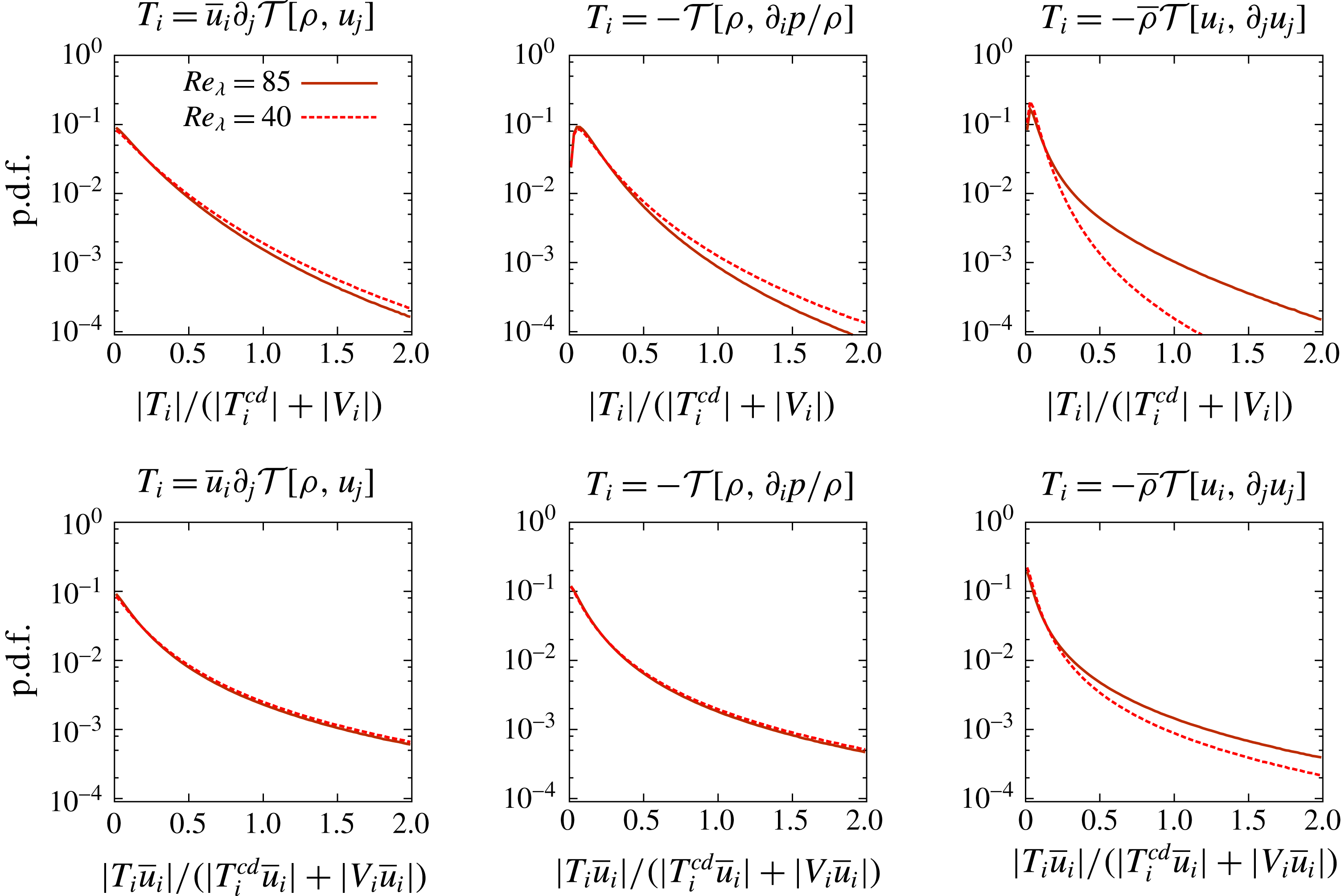
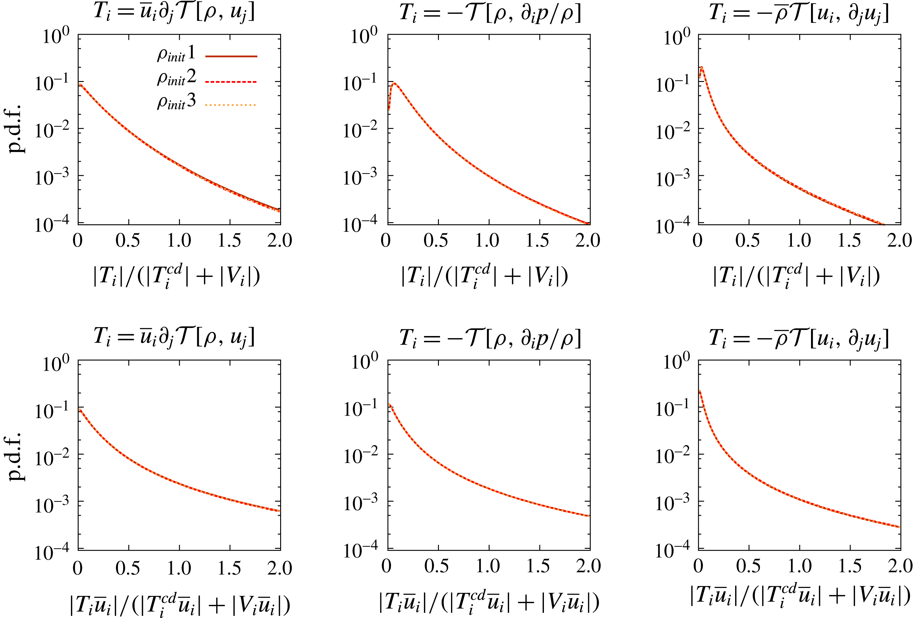
. The conclusions from the analysis are not sensitive to the time chosen in the decay regime. An exponential filter with
 $k_{c}\unicode[STIX]{x1D702}=0.12$
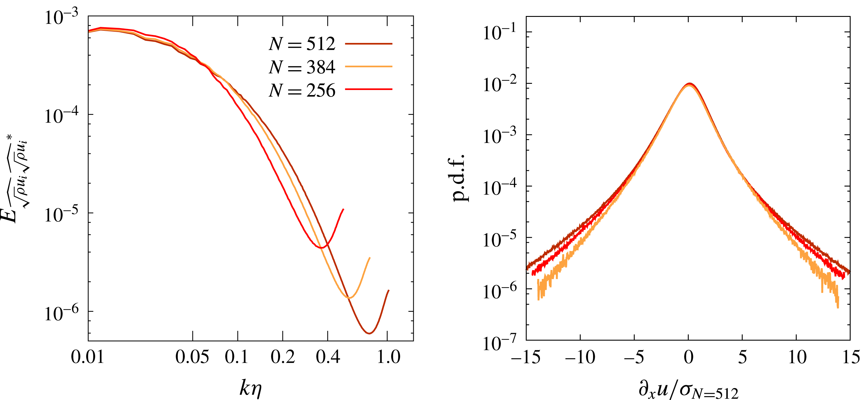
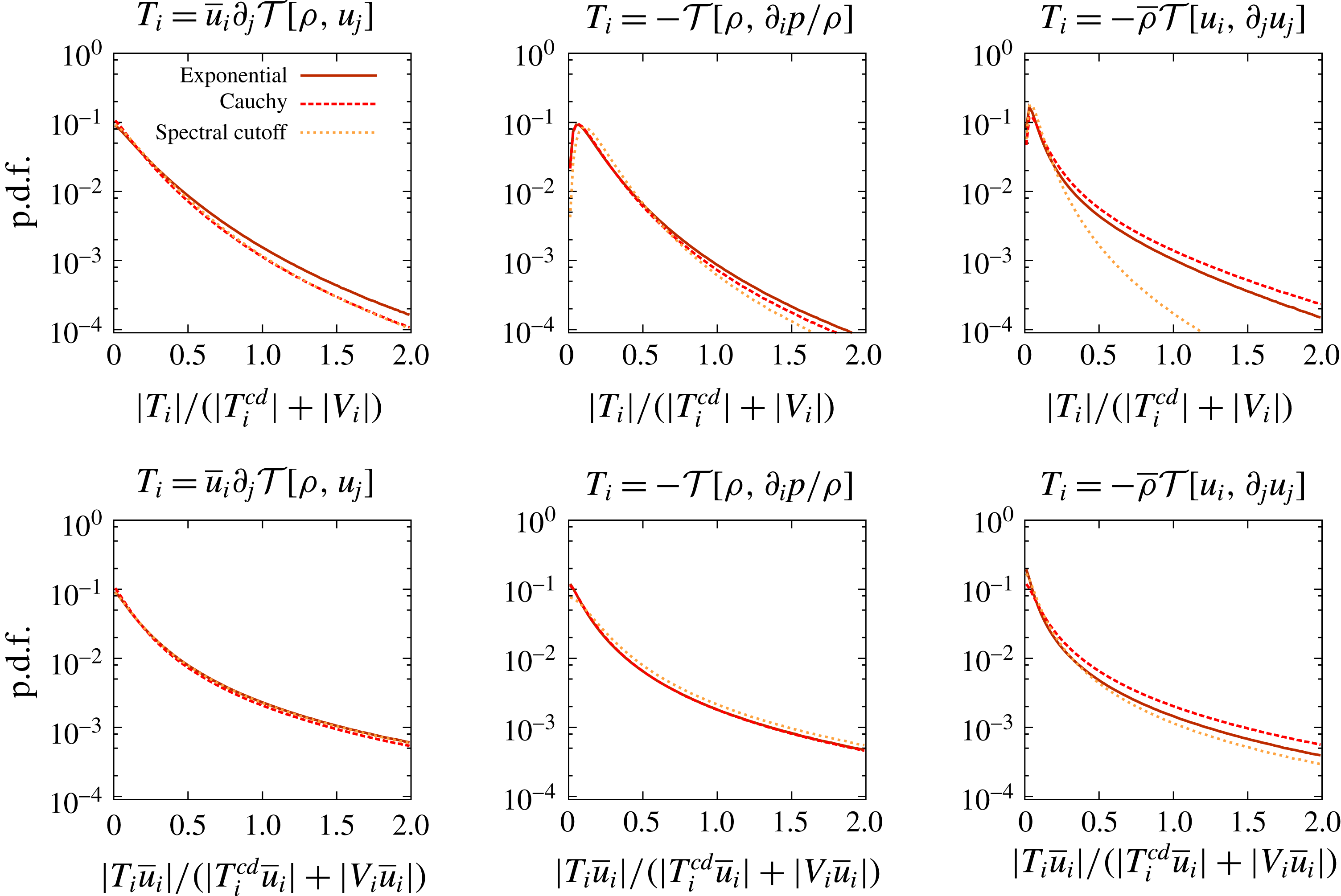
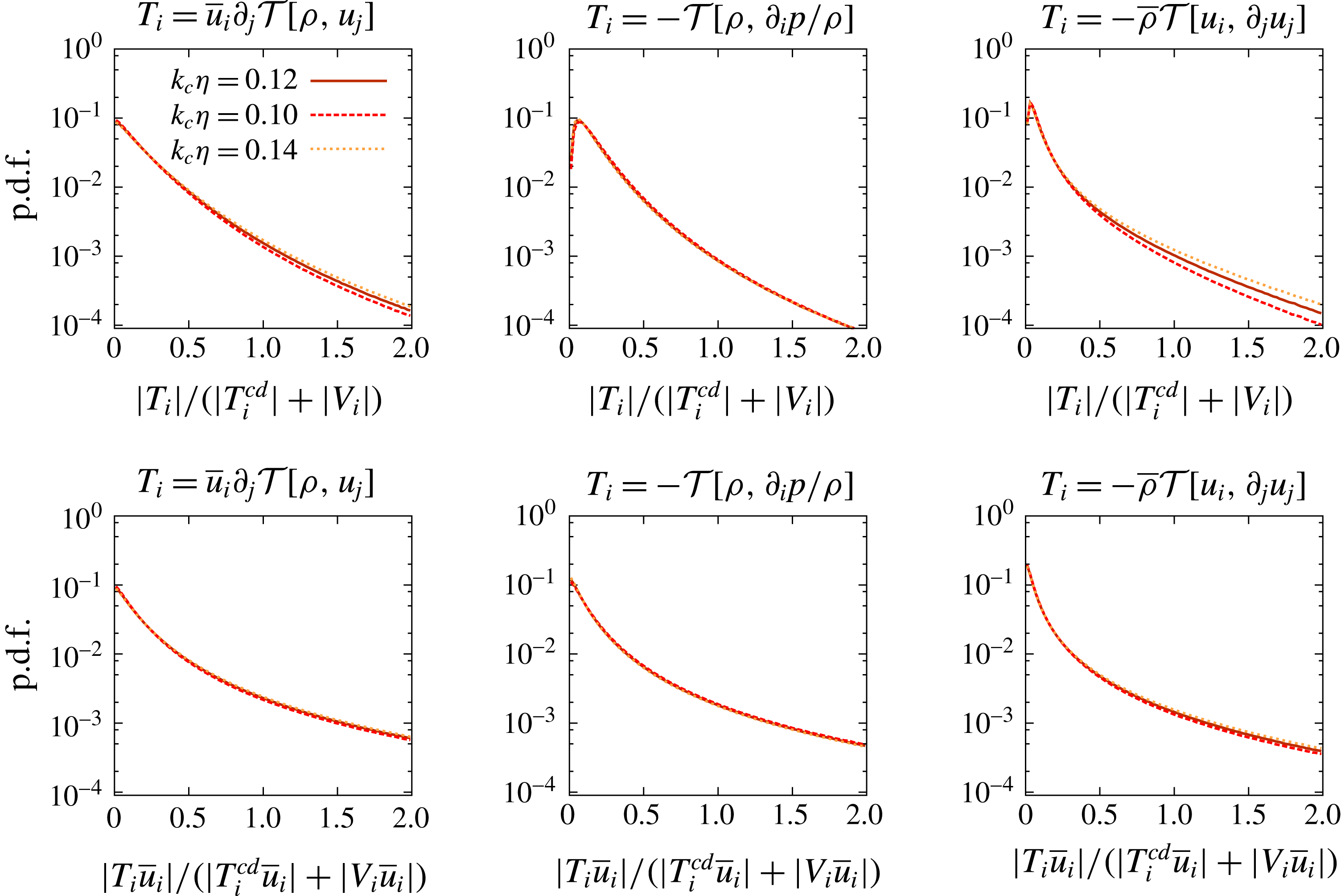
is used to filter the fields, and all filtering operations are carried out in Fourier space. The value of 0.12 is chosen so that the cutoff wavenumber lies in the inertial subrange and approximately 82 % of the kinetic energy is resolved. The effect of filter type and the choice of filter width is discussed in the Appendix. It is found that the relative importance of the variable-density SGS terms is not sensitive to either of these parameters.
4.1 Comparison of Reynolds-filtered and Favre-filtered velocity fields
The flow field corresponding to case 2b with an Atwood number of 0.7 is filtered to assess the differences between the
 $\tilde{u} _{i}$
and
 $\bar{u}_{i}$
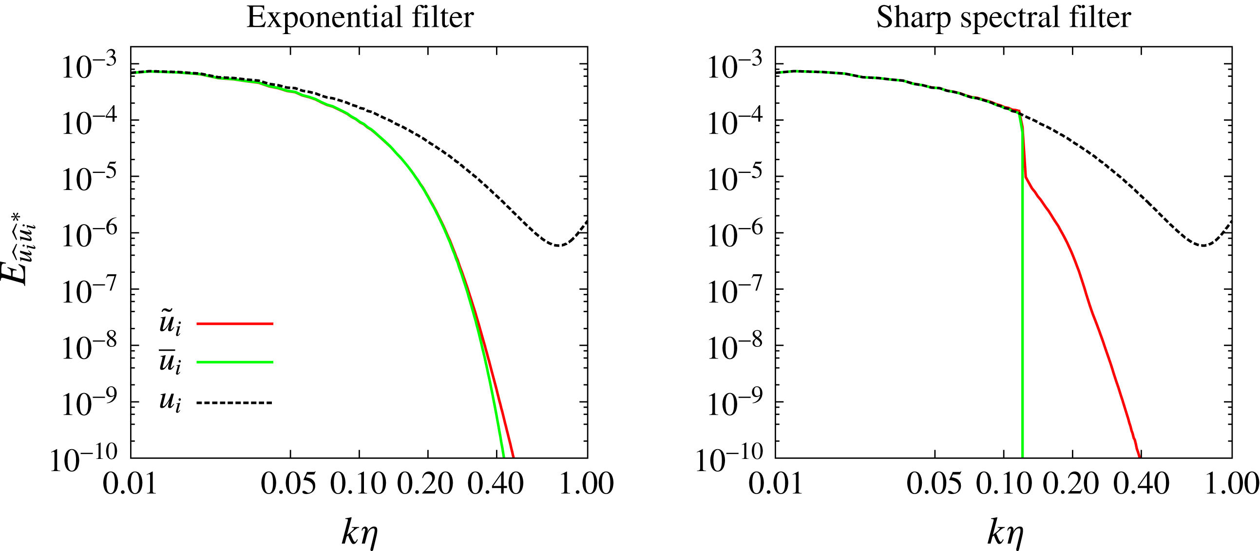
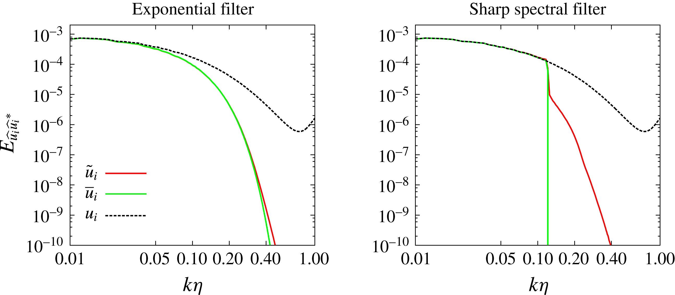
velocity fields. The spectral contents for both resolved-scale variables are found to be nearly identical for this case, with
 $\tilde{u} _{i}$
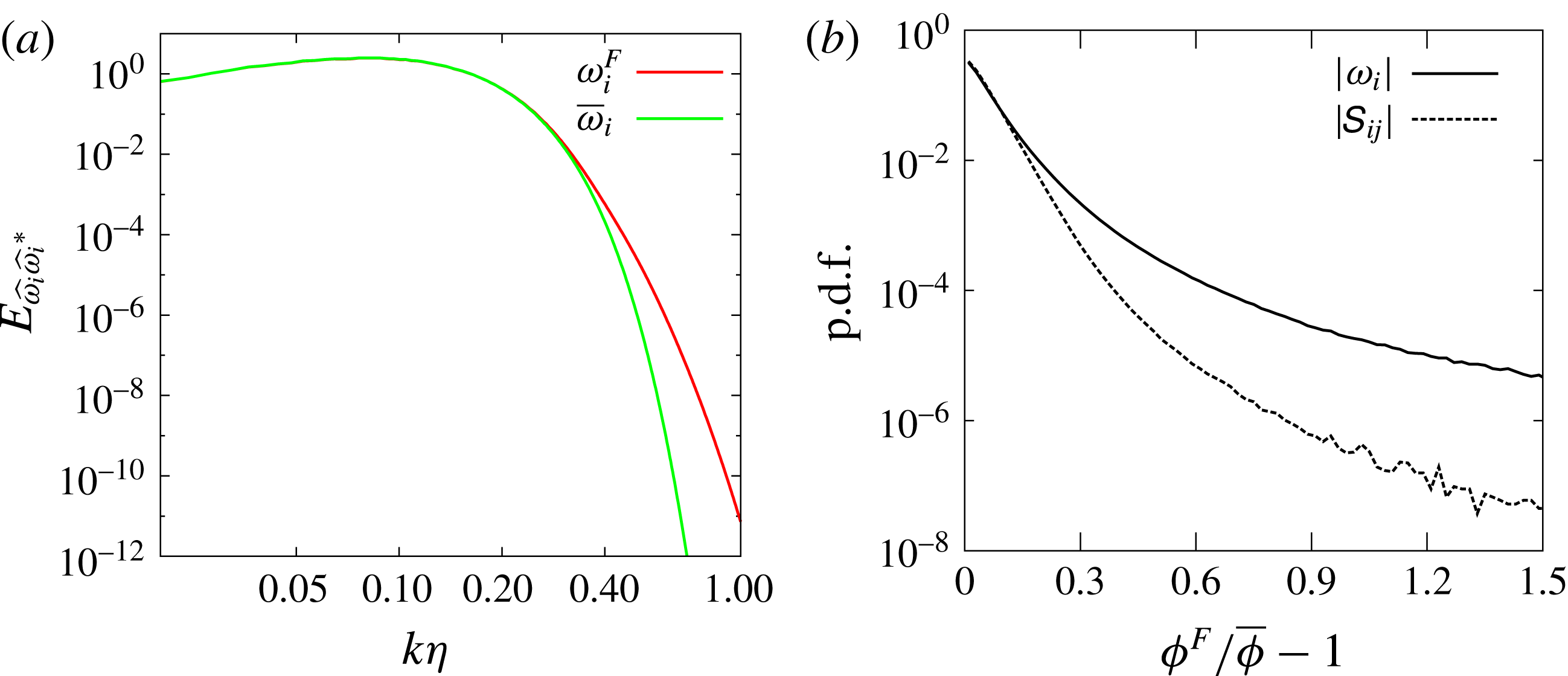
having slightly larger specific energy at wavenumbers beyond the filter cutoff (figure 5). This is true for the exponential and the sharp- spectral filter. We also compare the filtered vorticity
 $\bar{\unicode[STIX]{x1D714}}_{i}$
and the curl of the Favre-filtered velocity
 $\unicode[STIX]{x1D735}\times \tilde{u} _{i}$
in Fourier and physical space (figure 6
a). The curl of the Favre-filtered velocity
 $\unicode[STIX]{x1D714}_{i}^{\mathit{F}}=\unicode[STIX]{x1D735}\times \tilde{u} _{i}$
is referred to as pseudo-vorticity by Chakraborty et al. (Reference Chakraborty, Wang, Konstantinou and Klein2017). We also note that the pseudo-vorticity
 $\unicode[STIX]{x1D714}_{i}^{\mathit{F}}$
is not the Favre-filtered vorticity
 $\tilde{\unicode[STIX]{x1D714}}_{i}$
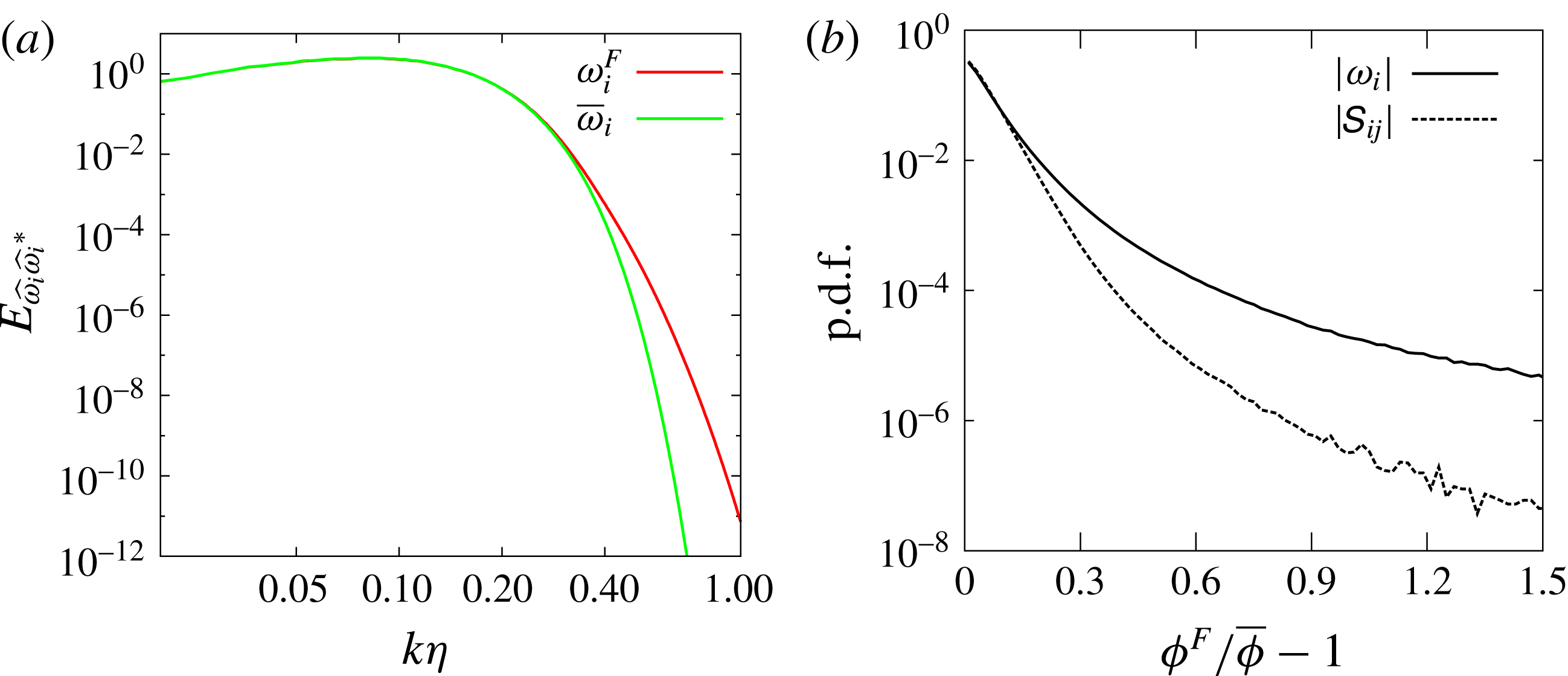
. The differences in the spectral contents of the filtered vorticity and pseudo-vorticity are found to be similar to the differences in the spectral contents of the velocity fields, except that they are amplified because
 $E_{\widehat{\unicode[STIX]{x1D714}}_{i}\widehat{\unicode[STIX]{x1D714}}_{i}^{\ast }}\sim k^{2}E_{\widehat{u_{i}}\widehat{u_{i}}^{\ast }}$
.
In physical space, the p.d.f. of the normalized difference between the
 $\bar{u}_{i}$
and
 $\tilde{u} _{i}$
gradient fields is plotted. It is found that the difference between
 $\bar{\unicode[STIX]{x1D714}}_{i}$
and
 $\unicode[STIX]{x1D714}_{i}^{\mathit{F}}$
can exceed 100 % in different regions of the flow. This is seen in figure 6(b), where
 $|\bar{\unicode[STIX]{x1D714}}_{i}|-|\unicode[STIX]{x1D714}_{i}^{\mathit{F}}|>|\bar{\unicode[STIX]{x1D714}}_{i}|$
(area under the solid curve beyond the horizontal-axis value of 1.0). The differences between the magnitudes of
 $\bar{\unicode[STIX]{x1D61A}}_{ij}$
and
 $\unicode[STIX]{x1D61A}_{ij}^{\mathit{F}}=1/2(\unicode[STIX]{x2202}_{i}\tilde{u} _{j}+\unicode[STIX]{x2202}_{j}\tilde{u} _{i})$
can also be large, but are relatively less pronounced than in the case of vorticity variables. In summary, the spectral contents of the Favre-filtered and Reynolds-filtered velocity fields in case 2b do not exhibit strong disparities in the decay stage. However, differences in the resolved-scale velocity-gradient fields in physical space are non-negligible.
Resolved-scale velocity radial spectra from case 2b filtered with
 $k_{c}\unicode[STIX]{x1D702}=0.12$
with different filters: the Favre-filtered velocity
 $\tilde{u} _{i}$
and the filtered velocity
 $\bar{u}_{i}$
are compared.
Comparison of the filtered vorticity
 $\bar{\unicode[STIX]{x1D714}}_{i}$
and the curl of the Favre-filtered velocity (
 $\unicode[STIX]{x1D714}_{i}^{\mathit{F}}=\unicode[STIX]{x1D735}\times \tilde{u} _{i}\neq \tilde{\unicode[STIX]{x1D714}}_{i}$
) (a), and the relative difference between
 $\bar{u}_{i}$
and
 $\tilde{u} _{i}$
gradient quantities in physical space (b).
4.2 Variable-density SGS terms in the resolved-scale momentum equation
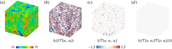
Case 2b: instantaneous density field at
 $t/t_{eddy}=3$
(a), and snapshots of fields corresponding to the SGS terms in the
 $\unicode[STIX]{x2202}_{t}\bar{\unicode[STIX]{x1D70C}}\tilde{u} _{1}$
equation (b–d). The SGS terms are non-dimensionalized by
 $|\langle \unicode[STIX]{x1D716}\rangle |/\sqrt{\langle u_{i}u_{i}/2\rangle }$
.

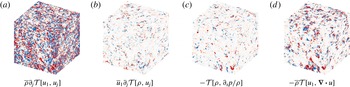
Case 2b: snapshots of fields corresponding to the SGS terms in the
 $\unicode[STIX]{x2202}_{t}\bar{\unicode[STIX]{x1D70C}}\bar{u}_{1}$
equation at
 $t/t_{eddy}=3$
(a–d). The legend is the same as figure 7.

The SGS terms in the resolved-scale momentum equation are computed using the DNS fields at
 $t/t_{eddy}=3.0$
with an exponential filter of
 $k_{c}\unicode[STIX]{x1D702}=0.12$
. The SGS terms involving the density
 $\unicode[STIX]{x1D70C}$
and dilatation
 $\unicode[STIX]{x1D735}\boldsymbol{\cdot }u$
in the central moments are of primary interest. The SGS specific stress
 ${\mathcal{T}}[u_{i},u_{j}]$
serves as the reference for comparison. The analysis is unique because the terms appearing in the resolved-scale momentum equation are considered, as opposed to terms appearing in the transport equations of SGS kinetic energy, SGS stress or other second-moment SGS terms. The resolved-scale momentum equations corresponding to both the variables,
 $\unicode[STIX]{x2202}_{t}\bar{\unicode[STIX]{x1D70C}}\tilde{u} _{i}$
and
 $\unicode[STIX]{x2202}_{t}\bar{\unicode[STIX]{x1D70C}}\bar{u}_{i}$
, are considered; each equation has its own set of SGS terms,
 $$\begin{eqnarray}{\displaystyle \frac{\unicode[STIX]{x2202}\bar{\unicode[STIX]{x1D70C}}\tilde{u} _{i}}{\unicode[STIX]{x2202}t}}+{\displaystyle \frac{\unicode[STIX]{x2202}}{\unicode[STIX]{x2202}x_{j}}}(\bar{\unicode[STIX]{x1D70C}}\tilde{u} _{i}\tilde{u} _{i}+\bar{p}\unicode[STIX]{x1D6FF}_{ij}+\bar{\unicode[STIX]{x1D70C}}{\mathcal{T}}[u_{i},u_{j}]+{\mathcal{T}}[\unicode[STIX]{x1D70C},u_{i},u_{j}]-{\mathcal{T}}[\unicode[STIX]{x1D70C},u_{i}]{\mathcal{T}}[\unicode[STIX]{x1D70C},u_{j}]/\bar{\unicode[STIX]{x1D70C}})=\bar{\unicode[STIX]{x1D70E}}_{\unicode[STIX]{x1D70C}u_{i}},\end{eqnarray}$$
 $$\begin{eqnarray}\displaystyle & & \displaystyle {\displaystyle \frac{\unicode[STIX]{x2202}\bar{\unicode[STIX]{x1D70C}}\bar{u}_{i}}{\unicode[STIX]{x2202}t}}+{\displaystyle \frac{\unicode[STIX]{x2202}}{\unicode[STIX]{x2202}x_{j}}}(\bar{\unicode[STIX]{x1D70C}}\bar{u}_{i}\bar{u}_{i}+\bar{p}\unicode[STIX]{x1D6FF}_{ij})+\bar{u}_{i}{\displaystyle \frac{\unicode[STIX]{x2202}{\mathcal{T}}[\unicode[STIX]{x1D70C},u_{j}]}{\unicode[STIX]{x2202}x_{j}}}+\bar{\unicode[STIX]{x1D70C}}{\displaystyle \frac{\unicode[STIX]{x2202}{\mathcal{T}}[u_{i},u_{j}]}{\unicode[STIX]{x2202}x_{j}}}-\bar{\unicode[STIX]{x1D70C}}{\mathcal{T}}\left[u_{i},{\displaystyle \frac{\unicode[STIX]{x2202}u_{j}}{\unicode[STIX]{x2202}x_{j}}}\right]\nonumber\\ \displaystyle & & \displaystyle \quad -{\mathcal{T}}\left[\unicode[STIX]{x1D70C},\frac{1}{\unicode[STIX]{x1D70C}}{\displaystyle \frac{\unicode[STIX]{x2202}p}{\unicode[STIX]{x2202}x_{i}}}\right]=\bar{\unicode[STIX]{x1D70E}}_{\unicode[STIX]{x1D70C}u_{i}}.\end{eqnarray}$$
The SGS terms arising from viscous transport, including
 ${\mathcal{T}}[\unicode[STIX]{x1D70C},\unicode[STIX]{x1D70E}_{\unicode[STIX]{x1D70C}u_{i}}/\unicode[STIX]{x1D70C}]$
, are not considered in this analysis. Snapshots of the
 $x$
component of the case 2b SGS vector field are shown in figures 7 and 8 for the
 $\unicode[STIX]{x2202}_{t}\bar{\unicode[STIX]{x1D70C}}\tilde{u} _{i}$
and
 $\unicode[STIX]{x2202}_{t}\bar{\unicode[STIX]{x1D70C}}\bar{u}_{i}$
equations respectively. All SGS terms are plotted on the same scale and colourmap. We see that the specific stress
 ${\mathcal{T}}[u_{i},u_{j}]$
terms in both equations are large and space-filling. While the variable-density SGS terms in both forms of the momentum equations are sparsely active, they can be large in specific regions. In particular, we note that the SGS mass flux term in the
 $\unicode[STIX]{x2202}_{t}\bar{\unicode[STIX]{x1D70C}}\tilde{u} _{i}$
equation is extremely small and that the SGS velocity-dilatation term is the most active variable-density SGS term in the
 $\unicode[STIX]{x2202}_{t}\bar{\unicode[STIX]{x1D70C}}\bar{u}_{i}$
equation.
The relative importance of the variable-density SGS terms is evaluated by normalizing by the local constant-density term. The resulting ratio fields quantify the importance of the variable-density SGS terms. Since the SGS terms are vectors, the ratios of scalar projections are evaluated; two scalars are considered for this purpose. The first scalar is the magnitude of the SGS vector. If we denote a particular variable-density SGS term by
 $T_{i}$
and the constant-density term by
 $T_{i}^{cd}$
, the quantity
 $|T_{i}|/|T_{i}^{cd}|$
indicates the relative magnitude. However, there are regions in the flow where
 $|T_{i}^{cd}|$
can approach zero, which corrupts the statistics. To avoid this issue, we evaluate the regularized ratio
 $|T_{i}|/(|T_{i}^{cd}|+|V_{i}|)$
, where
 $V_{i}=\bar{\unicode[STIX]{x1D70E}}_{\unicode[STIX]{x1D70C}u_{i}}$
is the resolved-scale viscous diffusion vector and represents a physical and dimensional regularization. Thus,
 $|V_{i}|$
ensures that the statistical information derived from the ratio field, particularly the p.d.f. tail, is not arbitrary. In comparison with the SGS terms
 $T_{i}$
, the
 $|V_{i}|$
values are typically very small. However, the
 $V_{i}$
field is space-filling and non-zero due to the presence of non-zero strain rate in the entire domain. In the limit when
 $k_{c}\unicode[STIX]{x1D702}\gg 1$
and the SGS terms are zero (
 $T_{i},T_{i}^{cd}\rightarrow 0$
), then
 $V_{i}\rightarrow \unicode[STIX]{x1D70E}_{\unicode[STIX]{x1D70C}u_{i}}$
, where
 $\unicode[STIX]{x1D70E}_{\unicode[STIX]{x1D70C}u_{i}}$
is the viscous term in the momentum equation. It should be noted that the SGS vectors require derivatives. Like the filters, we compute these derivatives in Fourier space.
Besides the magnitudes of these terms, a scalar incorporating the orientation of the SGS vectors is also required. In this context, projection on the resolved-scale velocity vector is considered. This is a physically meaningful projection and quantifies the contribution of SGS terms to the kinetic energy associated with the resolved-scale velocity. The rate of change of the kinetic energy is
 $$\begin{eqnarray}{\displaystyle \frac{\unicode[STIX]{x2202}\frac{1}{2}\bar{\unicode[STIX]{x1D70C}}\tilde{u} _{i}\tilde{u} _{i}}{\unicode[STIX]{x2202}t}}=\tilde{u} _{i}{\displaystyle \frac{\unicode[STIX]{x2202}\bar{\unicode[STIX]{x1D70C}}\tilde{u} _{i}}{\unicode[STIX]{x2202}t}}-\frac{1}{2}\tilde{u} _{i}\tilde{u} _{i}{\displaystyle \frac{\unicode[STIX]{x2202}\bar{\unicode[STIX]{x1D70C}}}{\unicode[STIX]{x2202}t}},\quad {\displaystyle \frac{\unicode[STIX]{x2202}\frac{1}{2}\bar{\unicode[STIX]{x1D70C}}\bar{u}_{i}\bar{u}_{i}}{\unicode[STIX]{x2202}t}}=\bar{u}_{i}{\displaystyle \frac{\unicode[STIX]{x2202}\bar{\unicode[STIX]{x1D70C}}\bar{u}_{i}}{\unicode[STIX]{x2202}t}}-\frac{1}{2}\bar{u}_{i}\bar{u}_{i}{\displaystyle \frac{\unicode[STIX]{x2202}\bar{\unicode[STIX]{x1D70C}}}{\unicode[STIX]{x2202}t}}.\end{eqnarray}$$
We see that the projection of the resolved-scale momentum equation SGS terms on the resolved-scale velocities is their contribution to the computable kinetic energy. The term
 $\bar{u}_{i}{\mathcal{S}}_{\unicode[STIX]{x1D70C}}$
appearing in
 $\unicode[STIX]{x2202}_{t}\bar{\unicode[STIX]{x1D70C}}\bar{u}_{i}$
is an exception; its contribution reverses sign due to the term
 $\unicode[STIX]{x2202}_{t}\bar{\unicode[STIX]{x1D70C}}$
. Similarly to the magnitude ratio, the ratio of the projection on the resolved-scale velocity is computed with
 $V_{i}$
to regularize the denominator. The ratio signifies the relative contribution to the resolved-scale kinetic energy.
Case 2b: the ratio p.d.f. computed for the trivariate moment magnitude in the
 $\unicode[STIX]{x2202}_{t}\bar{\unicode[STIX]{x1D70C}}\tilde{u} _{i}$
equation. The SGS terms are non-dimensionalized by
 $|\langle \unicode[STIX]{x1D716}\rangle |/\sqrt{\langle u_{i}u_{i}/2\rangle }$
. The inset is an isosurface enclosing regions where the ratio is greater than 0.5.

Probability distribution functions of the relative magnitude (a,c) and relative projection (b,d) for the SGS terms in the
 $\unicode[STIX]{x2202}_{t}\bar{\unicode[STIX]{x1D70C}}\tilde{u} _{i}$
equation from the instantaneous flow field.
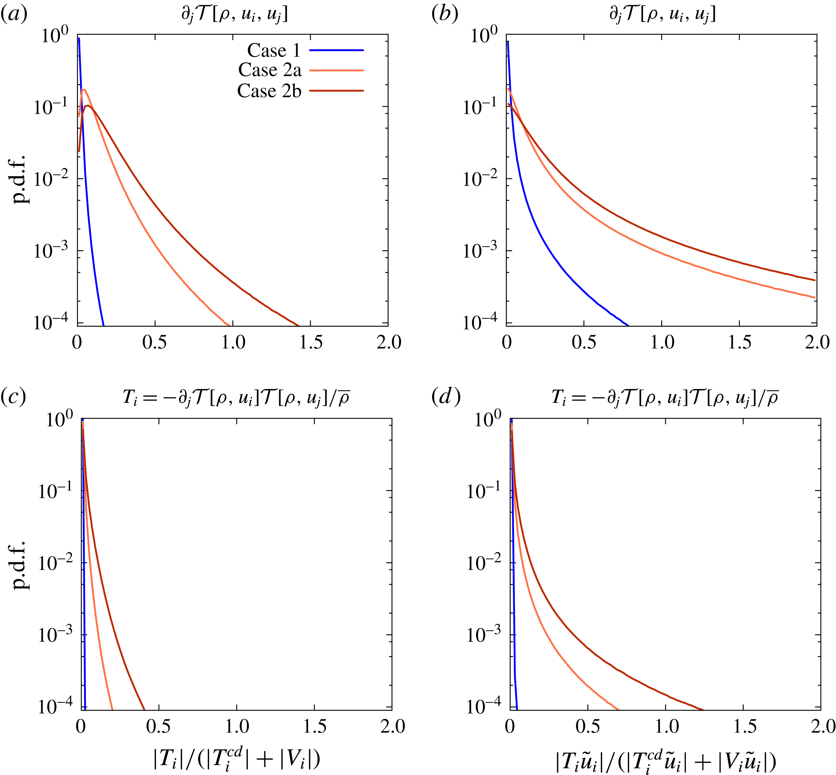
Probability distribution functions of the relative magnitude (a,c,e) and relative projection (b,d,f) for the SGS terms in the
 $\unicode[STIX]{x2202}_{t}\bar{\unicode[STIX]{x1D70C}}\bar{u}_{i}$
equation from the instantaneous flow field.
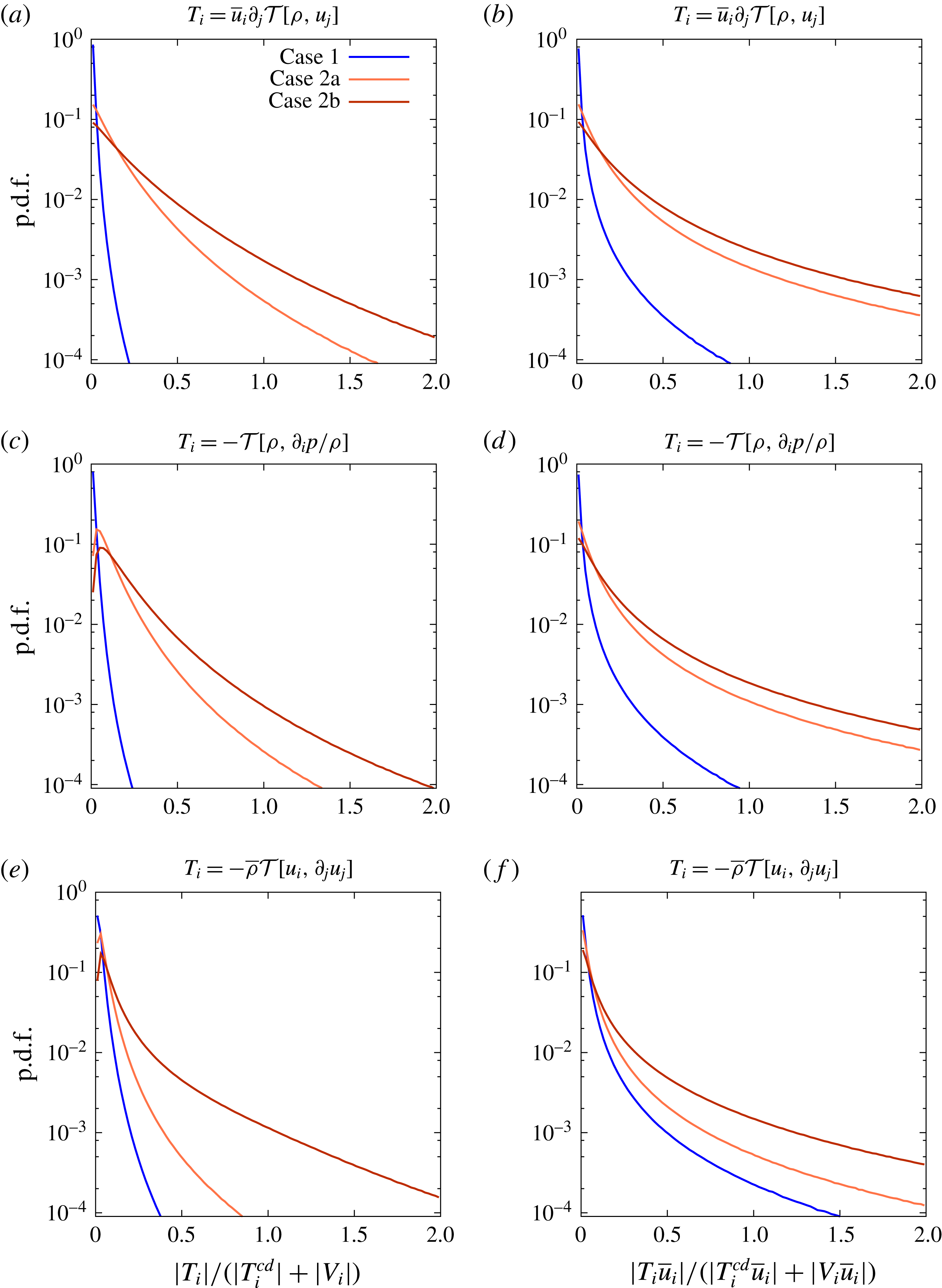
Conditional volumetric averages of the relative magnitude (black) and the relative projection (red) for the SGS terms in the Favre-filtered equation (a) and the Reynolds-filtered equation (b) from the instantaneous flow field.

Probability distribution functions of the relative magnitude (a) and the relative projection (b) for the SGS terms in the
 $\unicode[STIX]{x2202}_{t}\bar{\unicode[STIX]{x1D714}}_{i}$
equation from the instantaneous flow field.
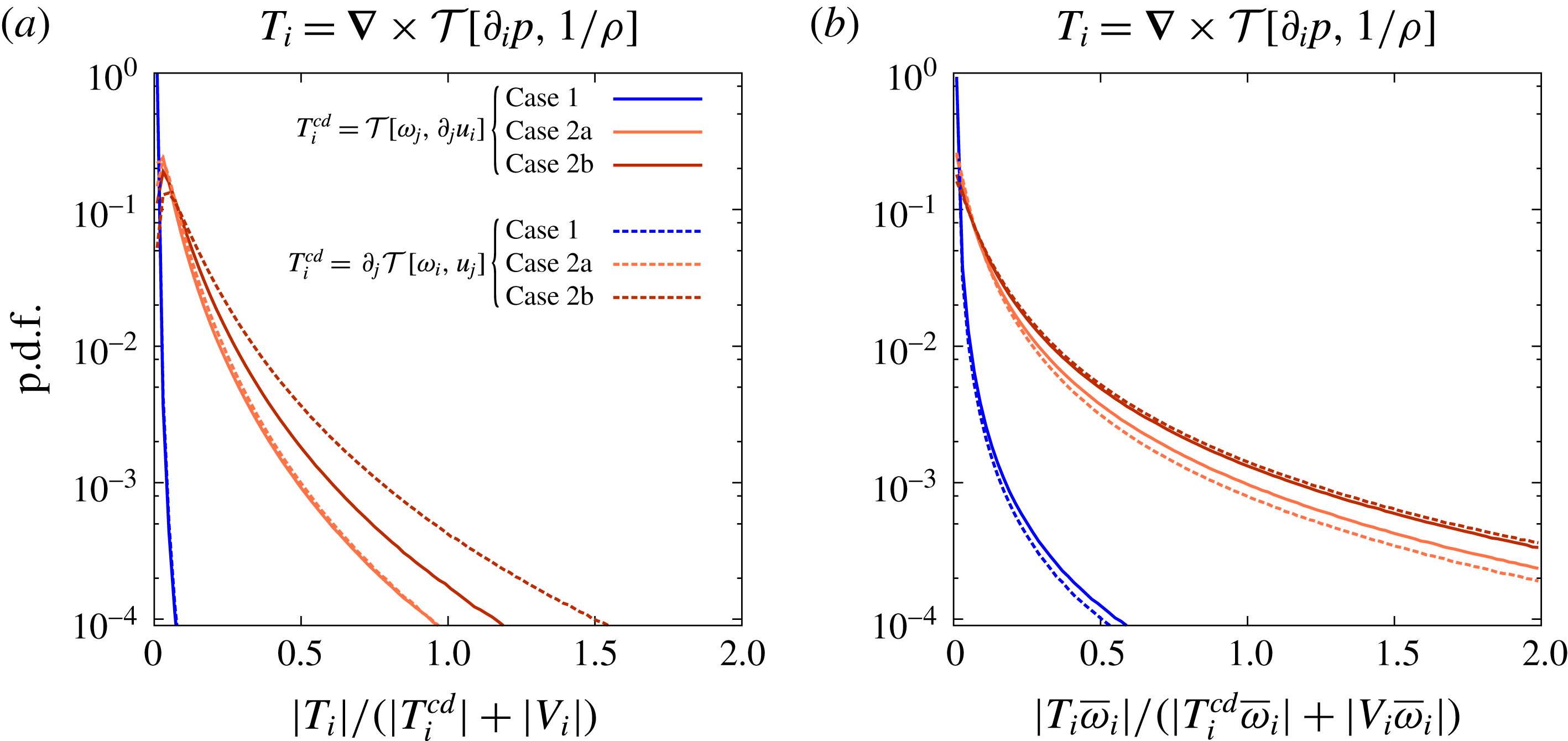
By computing the ratio at each point in the instantaneous flow field, we can compute the p.d.f.s for these fields. A typical ratio field and its p.d.f. are shown in figure 9. These distributions are plotted for
 $\tilde{u} _{i}$
(figure 10) and
 $\bar{u}_{i}$
(figure 11). Plots on the left are the magnitude ratio distributions, and plots on the right are the resolved-scale velocity projection ratios. Each plot has three curves with distributions from cases 1, 2a and 2b. Let us consider figure 10. The plots in panels (a) and (b) correspond to the trivariate moment term
 $\unicode[STIX]{x2202}_{j}{\mathcal{T}}[\unicode[STIX]{x1D70C},u_{i},u_{j}]$
and those in (c) and (d) correspond to the SGS mass flux term
 $-\unicode[STIX]{x2202}_{j}({\mathcal{T}}[\unicode[STIX]{x1D70C},u_{i}]{\mathcal{T}}[\unicode[STIX]{x1D70C},u_{j}]/\bar{\unicode[STIX]{x1D70C}})$
.
The Reynolds-filtered momentum equation
 $\unicode[STIX]{x2202}_{t}\bar{\unicode[STIX]{x1D70C}}\bar{u}_{i}$
p.d.f.s are plotted in figure 11 for the SGS mass flux term
 $\bar{u}_{i}\unicode[STIX]{x2202}_{j}{\mathcal{T}}[\unicode[STIX]{x1D70C},u_{j}]$
(a,b), the SGS pressure-gradient acceleration term
 $-{\mathcal{T}}[\unicode[STIX]{x1D70C},\unicode[STIX]{x2202}_{i}p/\unicode[STIX]{x1D70C}]$
(c,d) and the SGS velocity dilatation
 $\bar{\unicode[STIX]{x1D70C}}{\mathcal{T}}[u_{i},\unicode[STIX]{x2202}_{j}u_{j}]$
(e,f). All three variable-density SGS terms are found to be non-negligible for cases 2a and 2b, but insignificant for case 1. For both resolved-scale momentum variables, the terms are found to be more important by means of the velocity projection ratio metric.
Integral values for the ratios are also evaluated. The average ratio values are large for case 2b and small for case 1. For example, the value corresponding to the trivariate term in the Favre-filtered equation by the projection metric is 0.18 for case 2b and 0.01 for case 1. We note that averaging of the ratio field over the entire volume suppresses the importance of variable-density SGS terms as it causes the average to be biased by homogenized flow pockets where the ratio values are close to zero. Therefore, for case 2b, we present the conditionally averaged ratio in figure 12. The conditional average is the average over regions where
 $|\unicode[STIX]{x1D735}\bar{\unicode[STIX]{x1D70C}}|$
is greater than a specified value
 $|\unicode[STIX]{x1D735}\bar{\unicode[STIX]{x1D70C}}|_{c}$
. As the value of
 $|\unicode[STIX]{x1D735}\bar{\unicode[STIX]{x1D70C}}|_{c}$
is increased, the conditional mean of the ratios corresponding to all terms increases. This implies that when regions with strong density gradients are sampled, variable-density SGS terms become relatively more important, even in a statistical sense. For case 2b, the mean values of the variable-density terms are found to be larger than the specific stress term using the projection metric in regions of strong resolved-scale density gradients.
Ratio distributions for the filtered vorticity transport equation (2.28) are also computed. There are three inviscid SGS terms in the equation: the SGS vorticity flux
 $\unicode[STIX]{x2202}_{j}{\mathcal{T}}[\unicode[STIX]{x1D714}_{i},u_{j}]$
, the SGS vortex stretching term
 ${\mathcal{T}}[\unicode[STIX]{x1D714}_{j},\unicode[STIX]{x2202}_{j}u_{i}]$
and the SGS baroclinic torque
 $\unicode[STIX]{x1D735}\times {\mathcal{T}}[\unicode[STIX]{x2202}_{i}p,1/\unicode[STIX]{x1D70C}]$
. The p.d.f. plots quantifying the importance of the SGS baroclinic torque relative to the SGS vorticity flux
 $\unicode[STIX]{x2202}_{j}{\mathcal{T}}[\unicode[STIX]{x1D714}_{i},u_{j}]$
and the SGS vortex stretching term
 ${\mathcal{T}}[\unicode[STIX]{x1D714}_{j},\unicode[STIX]{x2202}_{j}u_{i}]$
are plotted in figure 13. Both metrics, magnitude and projection on
 $\bar{\unicode[STIX]{x1D714}}_{i}$
are considered. Projection of the SGS vectors onto the resolved-scale vorticity, similarly to the projection of the SGS terms in the momentum equation on the resolved-scale velocity, represents the contribution of each SGS term to the resolved-scale enstrophy
 $\bar{\unicode[STIX]{x1D714}}_{i}\bar{\unicode[STIX]{x1D714}}_{i}/2$
. The resolved-scale viscous term
 $\unicode[STIX]{x1D735}\times \bar{\unicode[STIX]{x1D70E}}_{\unicode[STIX]{x1D70C}u_{i}}/\bar{\unicode[STIX]{x1D70C}}$
is used for regularization of the denominator to compute the ratio fields. The ratios of SGS baroclinic torque to both SGS vorticity flux and SGS vortex stretching are computed, and are found to be important for cases 2a and 2b, but unimportant for case 1.
We now synthesize the important findings from the analysis. Turbulent flow fields with active variable-density effects have been investigated to quantify the role of variable-density SGS terms on the dynamics of the Favre-filtered and Reynolds-filtered velocity fields. Evidence for the significance of these terms is provided in the form of p.d.f.s of their magnitude relative to the constant-density SGS terms. Two scalar metrics are chosen to compare the SGS vectors, namely their magnitude and their contribution to kinetic-energy production and dissipation.
For the
 $M_{t}=0.3$
flows studied, it is found that density fluctuations arising out of compressibility alone are weak, and that SGS terms arising from small-scale density fluctuations are also negligible. However, when density fluctuations are associated with thermal inhomogeneities, they interact with the pressure-gradient field to produce acceleration fluctuations, thereby affecting velocity gradients. Not only is the vorticity affected, but the dilatation content is also significantly altered. Therefore, flow compressibility strongly couples with thermal-density inhomogeneities, and, consequently, the dynamics of compressible variable-density turbulence is inherently different from that of incompressible variable-density turbulence (Sandoval Reference Sandoval1995). Although we do not study compressible turbulent mixing of variable-density fluids with different molecular weights, such flows are expected to exhibit non-negligible variable-density SGS effects as well.
The analysis discusses variable-density effects on the Favre-filtered velocity SGS stress tensor in terms of central moments under the filter, which represent the spatial correlation between small scales. The trivariate moment
 ${\mathcal{T}}[\unicode[STIX]{x1D70C},u_{i},u_{j}]$
is found to be the most dynamically important variable-density term in the SGS stress. The physics of this term merits attention because it contributes significantly to the computable resolved-scale kinetic energy
 $\bar{\unicode[STIX]{x1D70C}}\tilde{u} _{i}\tilde{u} _{i}/2$
.
We also present an alternate form of the Reynolds-filtered Navier–Stokes equations. The equations are novel because they do not involve time derivatives of unclosed terms, and all unclosed terms involve only second moments under the filter operator. Using the new Reynolds-filtered momentum equation, we isolate the SGS inertial and dilatational effects and establish the dynamical importance of specific terms. The new Reynolds-filtered equations represent the effect of SGS pressure–acceleration, as well as the SGS mass flux and SGS dilatation correlations in resolved-scale mass, velocity and internal energy.
From the point of view of LES, the analysis has implications for the modelling of variable-density SGS effects. The new SGS terms provide a framework to study variable-density countergradient diffusion independently of the constant-density SGS terms. For example, in case 2b, we find that the SGS mass flux and SGS pressure acceleration terms have a net positive contribution to
 $(1/2)\unicode[STIX]{x2202}_{t}\bar{\unicode[STIX]{x1D70C}}\bar{u}_{i}\bar{u}_{i}$
, as opposed to the SGS specific stress, which has a net negative contribution. In other words, while the constant-density SGS term drains energy from the large scales in the mean sense, these two variable-density SGS terms transfer kinetic energy to the large scales. Countergradient diffusion is particularly important for turbulent combustion in which dilatation (Veynante et al.
Reference Veynante, Trouvé, Bray and Mantel1997; Yoshizawa et al.
Reference Yoshizawa, Fujiwara, Abe and Matsuo2009; O’Brien et al.
Reference O’Brien, Urzay, Ihme, Moin and Saghafian2014) and pressure gradients (Veynante & Poinsot Reference Veynante and Poinsot1997) correlate with countergradient diffusion of species and kinetic energy. Future work will involve the development and testing of SGS closures for the variable-density SGS terms in Favre- and Reynolds-filtered formulations in different classes of flows.
Comparison of decaying isotropic compressible turbulence simulations with literature (Lee, Lele & Moin Reference Lee, Lele and Moin1991; Samtaney et al. Reference Samtaney, Pullin and Kosović2001).
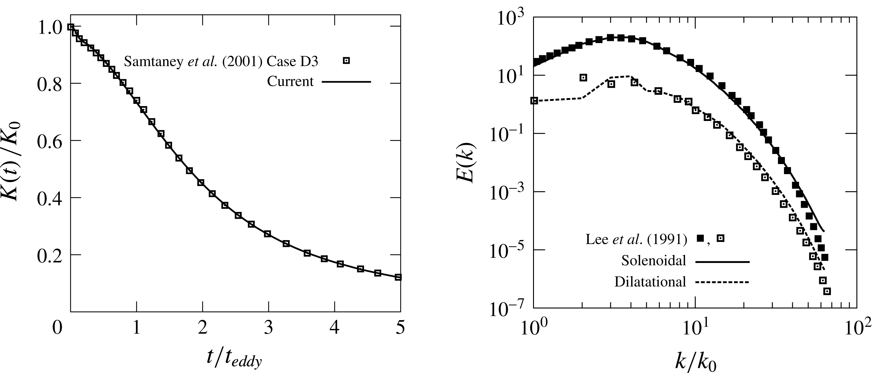
Grid refinement study of the field statistics at
 $t/t_{eddy}=3$
for case 2b.
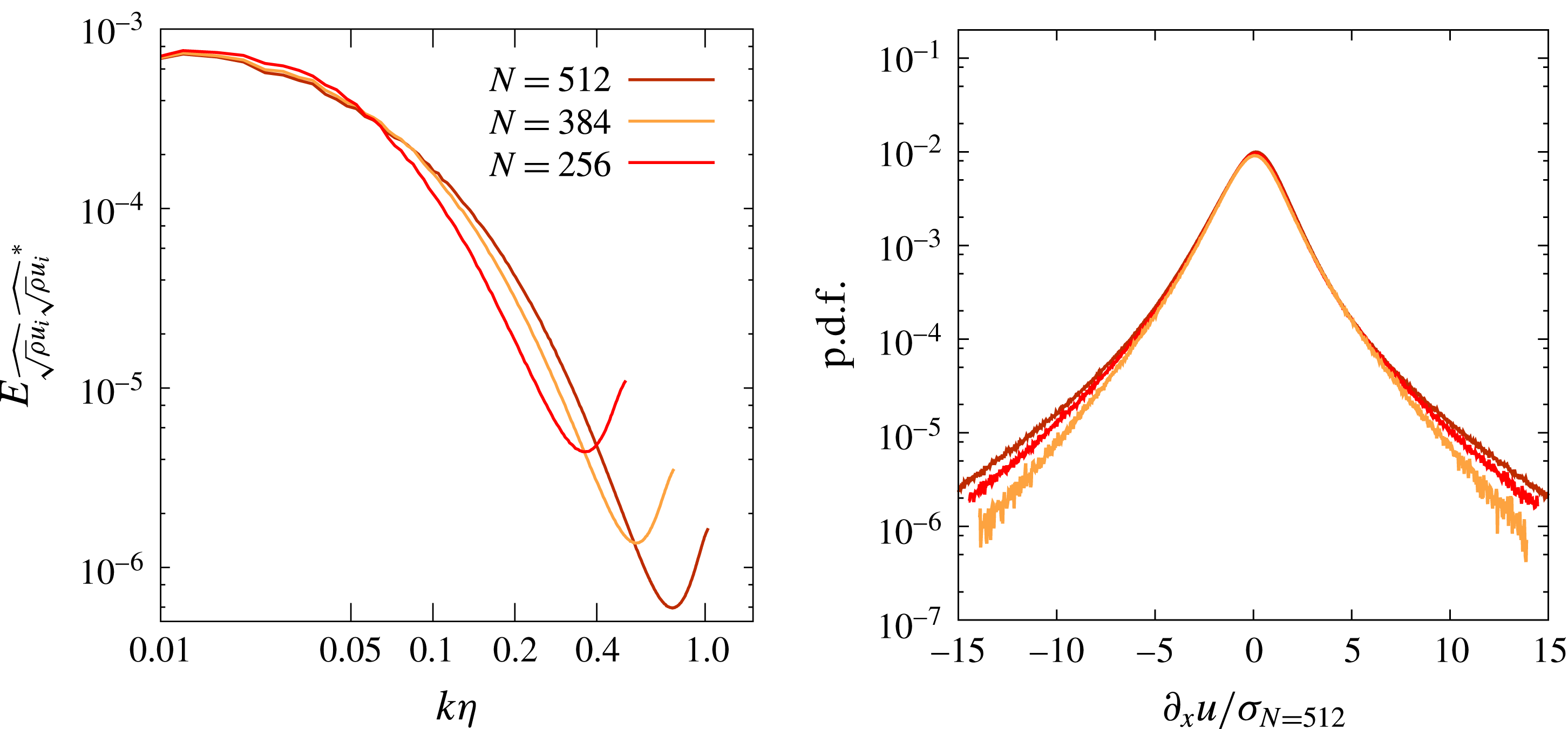
Effect of filter type on the relative strength of the variable-density SGS terms in the
 $\bar{\unicode[STIX]{x1D70C}}\bar{u}_{i}$
equation (case 2b).
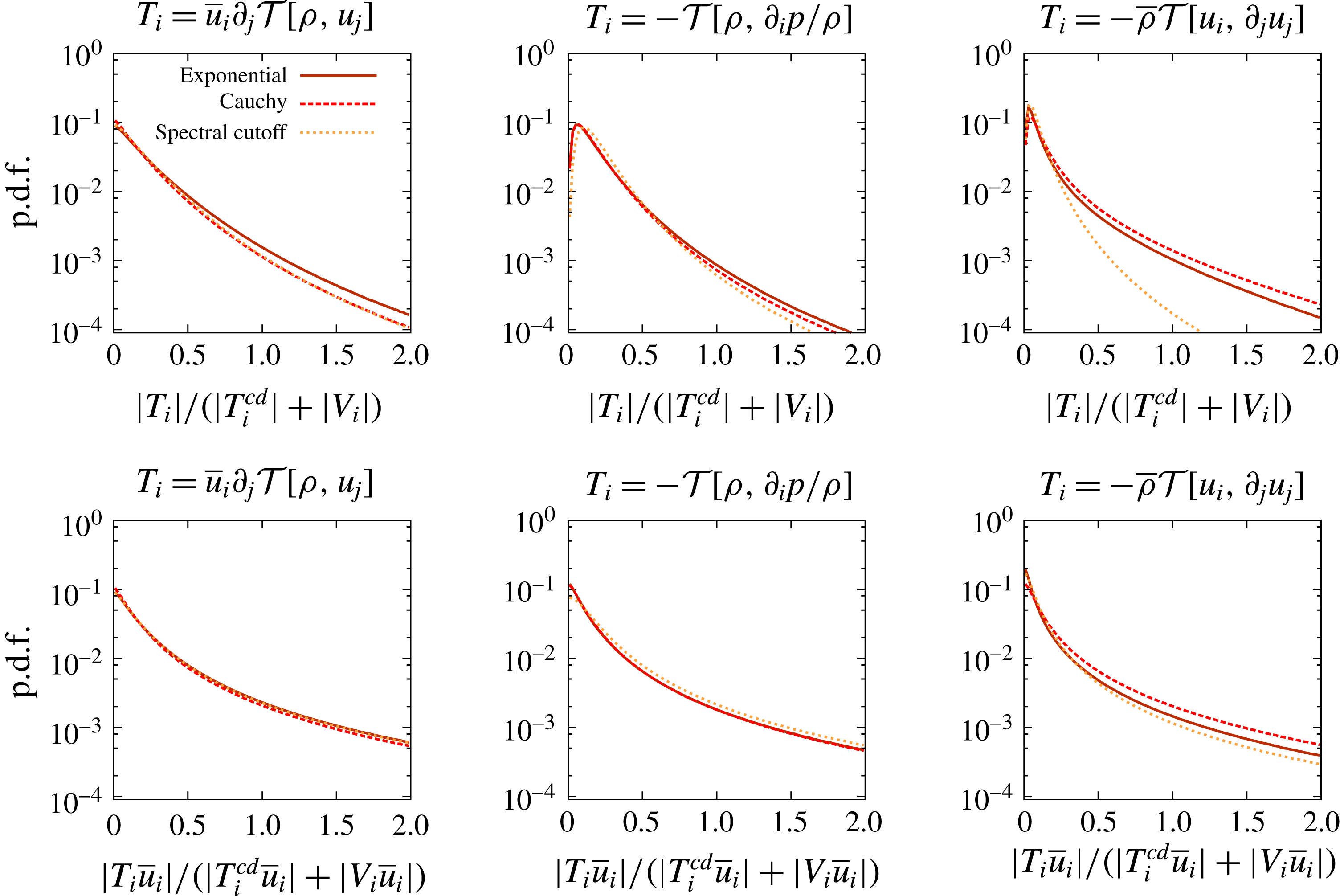
Effect of the cutoff wavenumber used in the exponential filter on the relative strength of the variable-density SGS terms in the
 $\bar{\unicode[STIX]{x1D70C}}\bar{u}_{i}$
equation (case 2b).
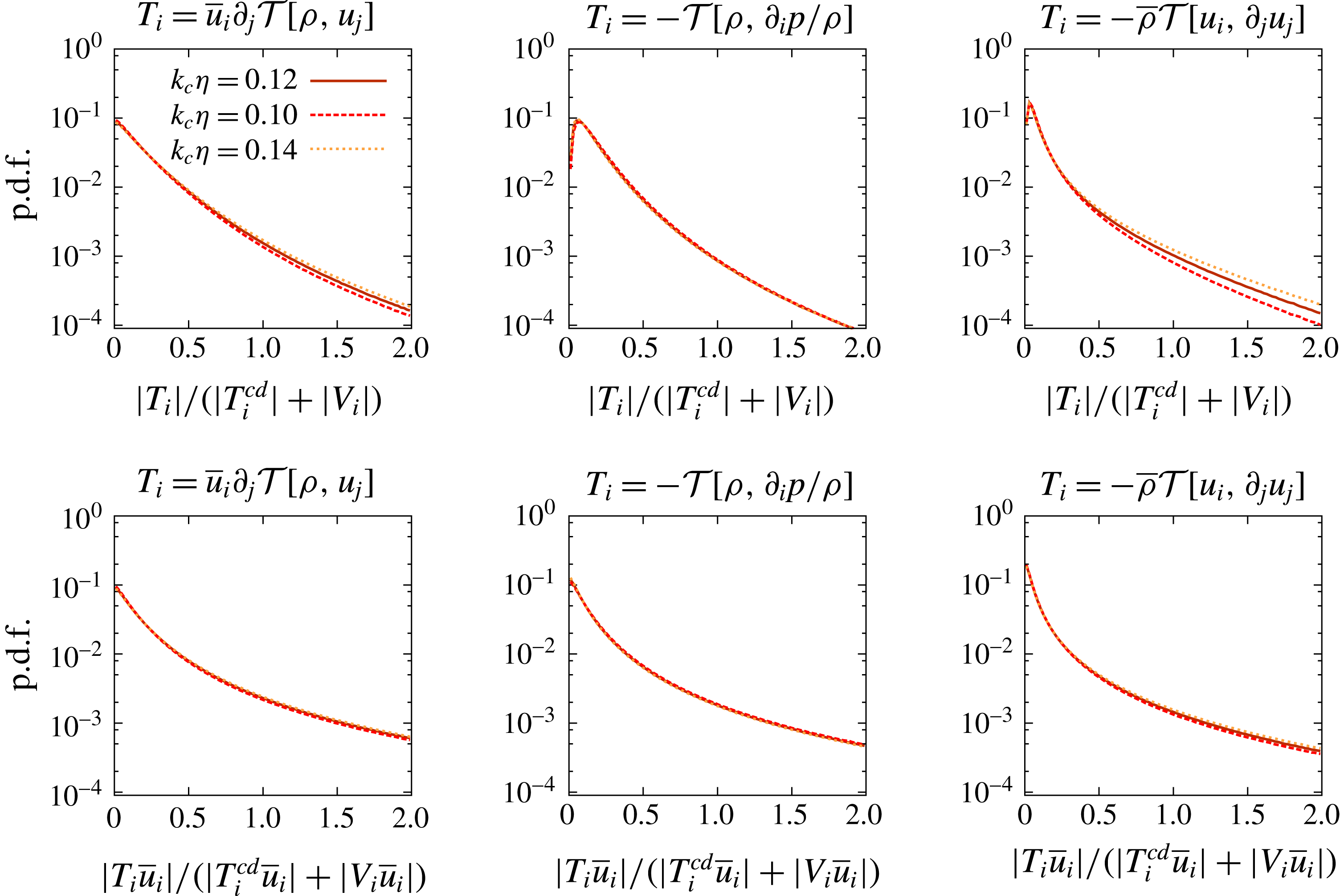
Effect of Reynolds number on the relative strength of the variable-density SGS terms in the
 $\bar{\unicode[STIX]{x1D70C}}\bar{u}_{i}$
equation. The Taylor scale Reynolds number shown in the plots corresponds to the instantaneous flow field (case 2b).
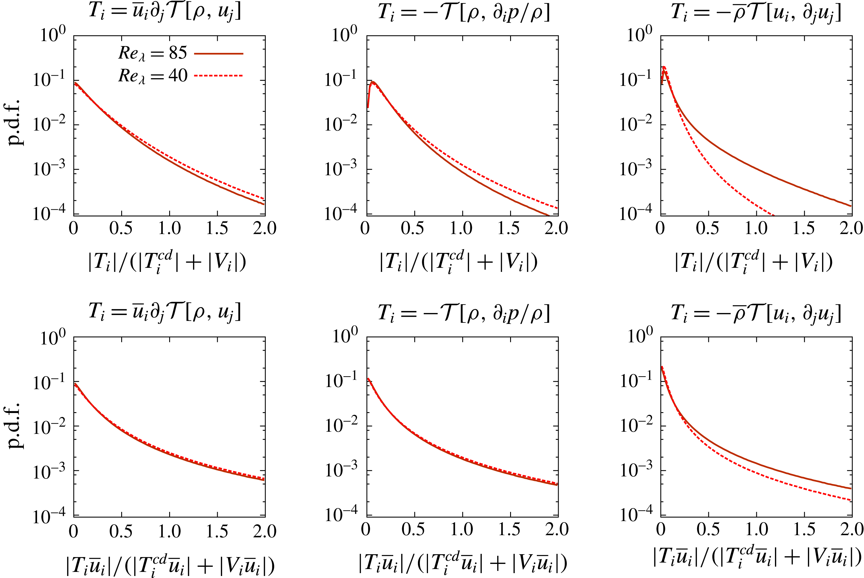
Effect of the randomness of the initial density field distribution on the relative strength of the variable-density SGS terms in the
 $\bar{\unicode[STIX]{x1D70C}}\bar{u}_{i}$
equation (case 2b).
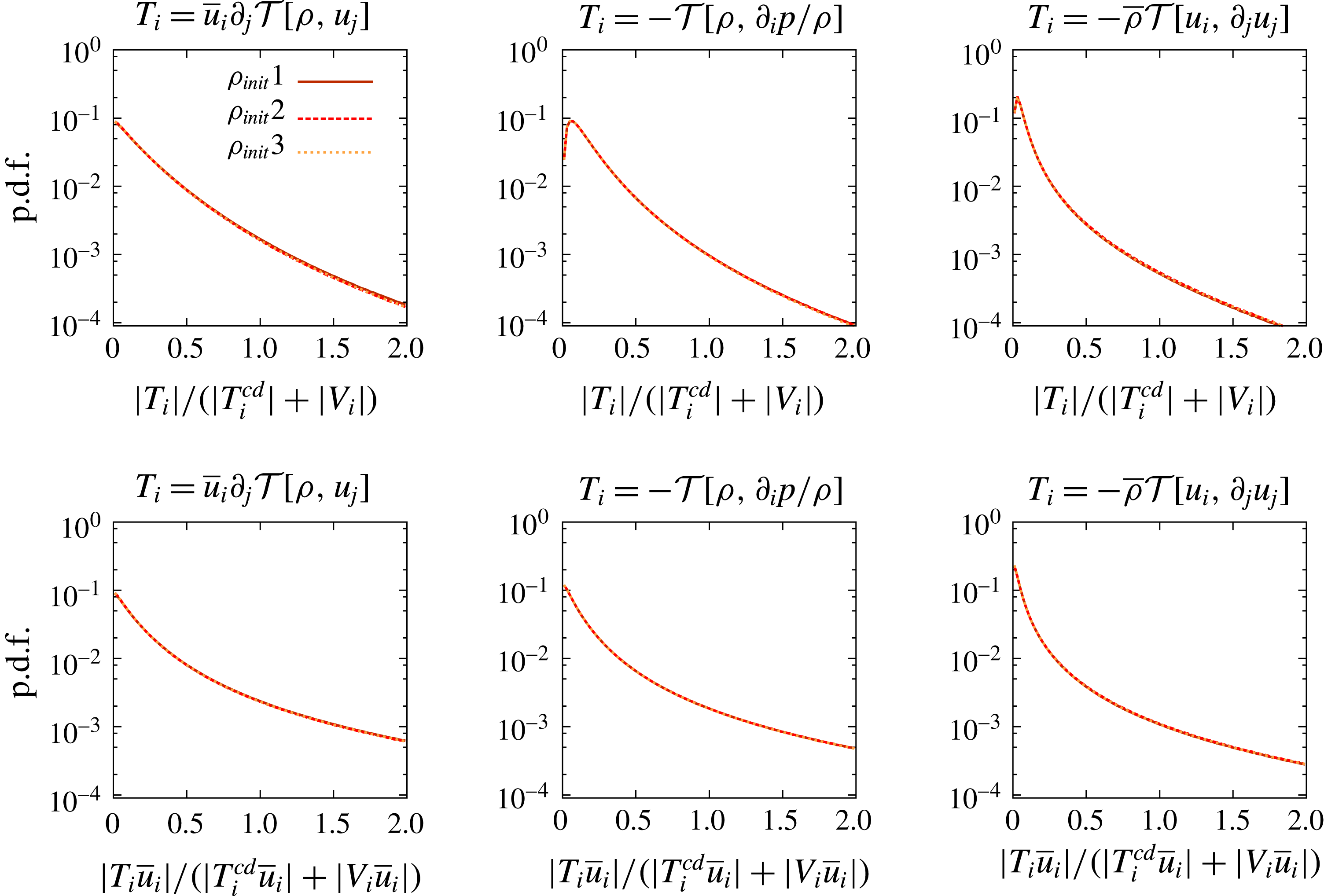
5 Conclusions
This paper identifies the role of SGS density fluctuations on the resolved-scale velocity, using both density-weighted and non-density-weighted forms of the governing equations. We first discuss the filtered Navier–Stokes equations in the conventional Favre-filtered framework and follow with a novel derivation of the Reynolds-filtered form of the equations. The filtered velocity dynamics is studied because the curl of the filtered velocity is the filtered vorticity. Important variable-density effects such as the SGS baroclinic torque appear in the transport equation of filtered vorticity. On the other hand, the curl of the Favre-filtered velocity follows different dynamics and can differ significantly from the filtered vorticity, particularly when small-scale density fluctuations are strong.
The conventional resolved-scale momentum equation derived without density weighting contains the time derivative of the SGS mass flux. This unsteady SGS term makes the equation cumbersome from a modelling perspective. Therefore, we derive a new set of Reynolds-filtered equations for mass, momentum and energy by decoupling the transport of SGS mass flux and SGS kinetic energy from the equations. In addition to having only spatial SGS terms, the new Reynolds-filtered equations involve only double correlations of the flow state.
In the equations for the resolved-scale momentum, we represent the SGS terms by expressing them as central moments under the filter operator. Using this method, we isolate the terms that involve the density or dilatation field, and the SGS terms containing only the specific stress
 $\overline{u_{i}u_{j}}-\bar{u}_{i}\bar{u}_{j}$
appear explicitly. We refer to such terms as constant-density SGS terms because they are the only active terms in a constant-density turbulent flow. After partitioning the SGS terms into variable-density and constant-density terms, it is natural to compare their relative strengths. For this purpose, we carry out DNS of two types of compressible decaying turbulence. In the first case, density fluctuations are primarily barotropic and arise from the compressibility of the flow, which is set to a moderate value. The other case involves the mixing of thermally inhomogeneous variable-density fluid regions with identical flow parameters. Therefore, the main content of the density fluctuations is entropic. It is found that the variable-density SGS terms are negligible in the first case, but important in the second case. This is attributed to the presence of strong inertial effects on small-scale turbulent flow features in the latter case.
We conclude that the effects of small-scale density variations on the dynamics of large-scale velocity and vorticity can be important in compressible flows involving the mixing of variable-density fluids. In the Favre-filtered momentum equation, these effects are embedded in the trivariate moment term (triple correlation), whereas, in the Reynolds-filtered momentum equation, these effects appear separately as the SGS pressure-gradient acceleration, the SGS velocity dilatation and the SGS mass flux convection. An understanding and quantification of the role played by these terms under different flow conditions will pave the way to the design of improved closures for variable-density turbulence.
Acknowledgements
We thank Dr P. Subbareddy and the reviewers for suggestions that improved the paper. This work was sponsored by the Air Force Office of Scientific Research under grant nos FA9550-12-1-0461 and FA9550-17-1-0250, and Department of Energy/National Nuclear Security Administration award no. DE-NA0002382. The views and conclusions contained herein are those of the authors and should not be interpreted as necessarily representing the official policies or endorsements, either expressed or implied, of the funding agencies or the U.S. Government.
Appendix
The sensitivity of the analysis to the choice of simulation and filtering parameters is briefly discussed in this section. A comparison of kinetic-energy decay and instantaneous radial spectra with simulations reported in the literature is shown in figure 14. The effect of the grid resolution on the case 2b flow field at a fixed time
 $t/t_{eddy}=3.0$
is shown in figure 15. The spectral content and the intermittency of the instantaneous flow field are properly captured with a grid resolution of
 $512^{3}$
. To quantify the sensitivity of the relative importance of the SGS variable-density terms, we focus on the resolved-scale momentum equation corresponding to the filtered velocity
 $\bar{u}_{i}$
. The effects of filter type, cutoff wavenumber for the exponential filter, initial and instantaneous length scale Reynolds number and the randomness of the initial density distribution are considered. The results are displayed in figures 16–19. The relative importance of the variable-density SGS terms is found to be insensitive to all of the parameters mentioned above, making the conclusions drawn in this paper general for decaying compressible variable-density turbulence.